The geometric link between Hardy and Clauser-Horne-Shimony-Holt

The idea proposed by Hardy is to construct a set of measurements on a bipartite state, such that a specific measurement outcome is predicted by quantum mechanics, which cannot be explained by classical physics.

For this purpose, we consider a bipartite two qubit state. On the subsystem $A$ we either perform the measurement $Q$ or $R$ which each can yield the outcome $+1$ or $-1$. Analogously, on the subsystem $B$ we choose between the two measurements $S$ and $T$.

The measurements are defined such that the joint probability measuring $Q=1$ and $T=1$ is zero. Furthermore, if one measures $S=1$, we always find $Q=1$ and analogously, if we measure $R=1$, one always finds $T=1$. The question is then, what is the joint probability to obtain $R=1$ and $S=1$ in a single measurement.

In any classical, local theory, the measurements on each subsystem do not influence each other and we change the measurement on a subsystem without changing the measurement outcome on the other subsystem.

We now assume that we find an outcome $R=1$ and $S=1$ in a single measurement. Then changing the measurement on the subsystem $A$ from $R$ to $Q$, we would obtain $Q=1$. In full analogy, if we change our measurement on the subsystem $B$ from $S$ to $T$, we would measure $T=1$.

As a consequence, if we changed the measurements on both subsystems simultaneously, the outcome of our new measurements would be $Q=1$ and $T=1$, which is in contradiction to the requirement, that the joint probability of $Q=1$ and $T=1$ is set to zero. Thus, for any classical theory, a common measurement of $R=1$ and $S=1$ cannot occur. This contradiction is schematically depicted in Figure 1.

However, it can be shown that quantum theory allows to construct measurements such that they obey the all of three requirements mentioned above, and still have a nonvanishing probability $w$ of finding $R=1$ and $S=1$ in the same run. We denote this situation as Hardy nonlocality. For a vivid interpretation of this scenario we refer to the work of Kwiat and Hardy Kwiat and Hardy 2000.

Therefore, in contrast to Bell inequalities, such as the CHSH inequality, in principle only a single measurement can suffice to violate the classical predictions. This behavior is similar to the famous Greenberger-Horne-Zeilinger (GHZ) scenario Greenberger et al. 1990 for three qubits and its extensions to multipartite multidimensional systems Cerf et al. 2002. However, in contrast to the GHZ model, the violation in the Hardy scenario only occurs probabilistically. Nevertheless, in any implementation, in order to guarantee the other three conditions, one theoretically needs to perform infinitely many measurements.

Our article is organized in the following way. In Sec. II we formulate the Hardy scenario in a quantum mechanical formalism and show how it is related to the CHSH inequality plus additional constraints. We then develop a geometrical interpretation of the probability $w$ in Sec. III. We exploit this interpretation in Sec. IV to optimize the nonlocality probability $w$, and determine the optimal measurement settings in Sec. V. In Sec. VI, we compare our findings for the Hardy scenario to the results for the CHSH scenario, and discuss how the different constraints in the Hardy scenario effect the results found. Finally, we provide a conclusion in VII.

In order to keep our article self-containing but focused on the main results, we provide three appendices. In Appendix A we calculate the relations between the different measurement vectors due to the additional constraints. We devote Appendix B to obtaining an analytical expression for the expected correlation value in terms of spherical coordinates. We finally provide a derivation of the violation probability in terms of a length appearing in our geometrical picture in Appendix C.

We first define the quantum mechanical state and measurements and translate the classical probabilities of the Hardy problem, presented in Section I, into quantum mechanical probabilities.

Throughout the remainder of this article, we consider a pure two-qubit state

in the Schmidt basis János A. Bergou 2013, where $\left|0\right\rangle$ and $\left|1\right\rangle$ are the eigenstates of the Pauli $\hat{\sigma}_{z}$ operator with eigenvalue $+1$ and $-1$ in the respective subsystem. Furthermore, the concurrence $\mathcal{C}$ Wootters 1998; Rungta et al. 2001, with $0\leq\mathcal{C}\leq 1$ is a measure of the entanglement between the two subsystems of the two-qubit state. For $\mathcal{C}=0$ the state is separable, while $\mathcal{C}=1$ is a maximally entangled Bell state.

We note that the state $\left|\Psi\right\rangle$ is an arbitrary state with given entanglement, that is any other state with the same entanglement can be transformed into Equation 1 by a change of basis.

Due to the symmetry of the state $\left|\Psi\right\rangle$ in the Schmidt basis, the Bloch vectors $\boldsymbol{a}_{A}=\left\langle\Psi\right|\hat{\boldsymbol{\sigma}}_{A}\left|\Psi\right\rangle$ and $\boldsymbol{a}_{B}=\left\langle\Psi\right|\hat{\boldsymbol{\sigma}}_{B}\left|\Psi\right\rangle$ of the two subsystems $A$ and $B$, where $\hat{\boldsymbol{\sigma}}$ is the vector of the Pauli matrices $\hat{\sigma}_{x}$, $\hat{\sigma}_{y}$ and $\hat{\sigma}_{z}$, have the same representation

and we drop the indices in the following.

On each of the two subsystems we perform one of two possible measurements. On the subsystem $A$, we choose between the operators

where $\boldsymbol{q}$ and $\boldsymbol{r}$ are three-dimensional unit vectors that denote the measurement direction on the Bloch sphere of the subsystem $A$.

In full analogy, on the subsystem $B$ we perform either the measurement

with the three-dimensional unit vectors $\boldsymbol{s}$ and $\boldsymbol{t}$.

From these measurement settings, we derive the sum of expectation values

of the individual measurement correlations. Inserting the state $\left|\Psi\right\rangle$, Equation 1, and the measurement operators, Equations 3 and 4, into Equation 5, we obtain the expectation value

in terms of the measurement vectors $\boldsymbol{q}$, $\boldsymbol{r}$, $\boldsymbol{s}$ and $\boldsymbol{t}$ and the correlation matrix

which is a property of the state alone. For the state $\left|\Psi\right\rangle$, Equation 1, the correlation matrix is explicitly given by

where the diagonal form of the matrix is a direct consequence of using the Schmidt decomposition. Note, that $K\boldsymbol{a}=\boldsymbol{a}$, since $\boldsymbol{a}$ points along the $z$ axis.

For any classically correlated, local system, the CHSH inequality

holds. However, Equation 9 can be violated for entangled quantum mechanical states. Indeed, for a state with concurrence $\mathcal{C}$, the expectation value is bounded by

for any CHSH like experiment. Only for separable states ($\mathcal{C}=0$) a violation of the CHSH inequality is impossible. For maximally entangled states, that is $\mathcal{C}=1$, we find $\mathcal{S}\leq 2\sqrt{2}$, the well-known Tsirelson bound Cirel'son 1980; Tsirel'son 1987.

In contrast to the CHSH inequality, the idea of the Hardy scenario is to prepare the above measurements in such a way, that we guarantee them to fulfill the three probability distributions for the outcomes $Q,R,S$ and $T$ associated with a single measurement of the operator $\hat{Q},\hat{R},\hat{S}$ and $\hat{T}$, discussed in Section I.

The first condition is that the joint probability

of simultaneous measurement of $\hat{Q}$ and $\hat{T}$ on the two subsystems of the state $\left|\Psi\right\rangle$ cannot yield the outcome $1$ on both sides.

The second requirement is finding the outcome $S=1$ when measuring $\hat{S}$ on subsystem $B$ will definitely result in the outcome $Q=1$ for a measurement of $\hat{Q}$, that is we have the conditional probability

In full analogy to the second condition, the third is the conditional probability

which predicts that we find $T=1$ on the subsystem $B$, when we measured $R=1$ on the subsystem $A$.

We then ask the question, what is the probability

of the joint measurement outcomes $R=1$ and $S=1$.

As we have discussed in the introduction, if our measurement settings fulfill Equations 11, 12 and 13, obtaining a single measurement outcome with $R=1$ and $S=1$ in the same measurement is a violation of any local hidden variable theory.

Inserting the definitions of our state $\left|\Psi\right\rangle$, Equation 1, and measurement operators, Equations 3 and 4, into the definition of the joint and conditional probabilities, Equations 11, 12, 13 and 14, we obtain a set of four equations:

which only depend on the measurement vectors $\boldsymbol{q},\boldsymbol{r},\boldsymbol{s}$ and $\boldsymbol{t}$, the Bloch vector $\boldsymbol{a}$, and the correlation matrix $K$.

We are now in the position to compare the Hardy scenario with the CHSH inequality. In order to do so, we add Equations 16, 17 and 18 and subtract Equation 15, and obtain

We identify the left hand side of Equation 19 as the expectation value $\mathcal{S}$, Equation 6, at the heart of the CHSH inequality.

Hence, the probability

of finding a measurement outcome that contradicts the locality condition is directly connected to the violation of the CHSH inequality, Equation 9. If and only if the measurement setting would violate this inequality, it is possible to obtain a measurement of $Q=1$ and $S=1$ in the same run. For this reason, we call $w$ the violation probability.

In order to maximize $w$, we simply have to maximize the expectation value $\mathcal{S}$, which corresponds to maximizing the violation of the CHSH inequality.

The maximization of $\mathcal{S}$ over the four independent measurements $\boldsymbol{q}$, $\boldsymbol{r}$, $\boldsymbol{s}$ and $\boldsymbol{t}$ for a pure state is known Gisin 1991. We even demonstrated a geometrical approach Seiler et al. 2021 which allows one to find all possible measurement that maximize $\mathcal{S}$ for a given concurrence $\mathcal{C}$.

However, in addition to Equation 20, the probabilities Equations 11, 12 and 13 between correlated measurement outcomes still must be fulfilled. As a consequence the measurement vectors $\boldsymbol{q}$, $\boldsymbol{r}$, $\boldsymbol{s}$ and $\boldsymbol{t}$ are no longer independent of each other.

Unfortunately, as it turns out none of the infinitely many optimal measurement settings for maximizing $\mathcal{S}$ for a given concurrence $\mathcal{C}$ without any further constraints fulfills the three additional constraints, Equations 24, 25 and 26, on the measurement vectors. In order to maximize $w$, the expectation value thus has to be maximized again under these new constraints.

We now take a closer look at the additional constraints, which arise from demanding the probabilities Equations 11, 12 and 13.

The first constraint, Equation 15, leads to

which we rewrite as

where $\alpha$ is the angle between $\boldsymbol{t}$ and $K\boldsymbol{q}+\boldsymbol{a}$. The premise of $\boldsymbol{t}$ being a unit vector, together with the relation

which is proven in Appendix A, then constitute that the measurement vector $\boldsymbol{t}$ is antiparallel to $K\boldsymbol{q}+\boldsymbol{a}$, leading to the connection

between the vectors $\boldsymbol{q}$ and $\boldsymbol{t}$.

The second constraint, Equation 16, leads to the connection

between the vectors $\boldsymbol{q}$ and $\boldsymbol{s}$.

Analogously, we find

between the vectors $\boldsymbol{r}$ and $\boldsymbol{t}$ from the third constraint, Equation 17.

As a consequence, instead of four independent vectors $\boldsymbol{q}$, $\boldsymbol{r}$, $\boldsymbol{s}$ and $\boldsymbol{t}$, the three vectors $\boldsymbol{r}$, $\boldsymbol{s}$ and $\boldsymbol{t}$ are fully determined by the vector $\boldsymbol{q}$. We only have one independent vector $\boldsymbol{q}$ left.

The expectation value $\mathcal{S}$, Equation 6, under the constraints Equations 24, 25 and 26, and hence the probability $w$, Equation 20, is a function of only a single measurement vector.

In order to maximize the probability $w$, we parameterize the measurement vector

in spherical coordinates by two angles $\theta$ and $\phi$ and insert the resulting expression together with the expressions for the other three vectors $\boldsymbol{r},\boldsymbol{s},\boldsymbol{t}$, Equations 25, 24 and 26, and the correlation matrix $K$, Equation 8, into the definition of the expectation value $\mathcal{S}$, Equation 30. The resulting expression for the expectation value, given in Appendix B, only depends on the angle $\theta$ and the concurrence $\mathcal{C}$, but is rather cumbersome and difficult to maximize analytically.

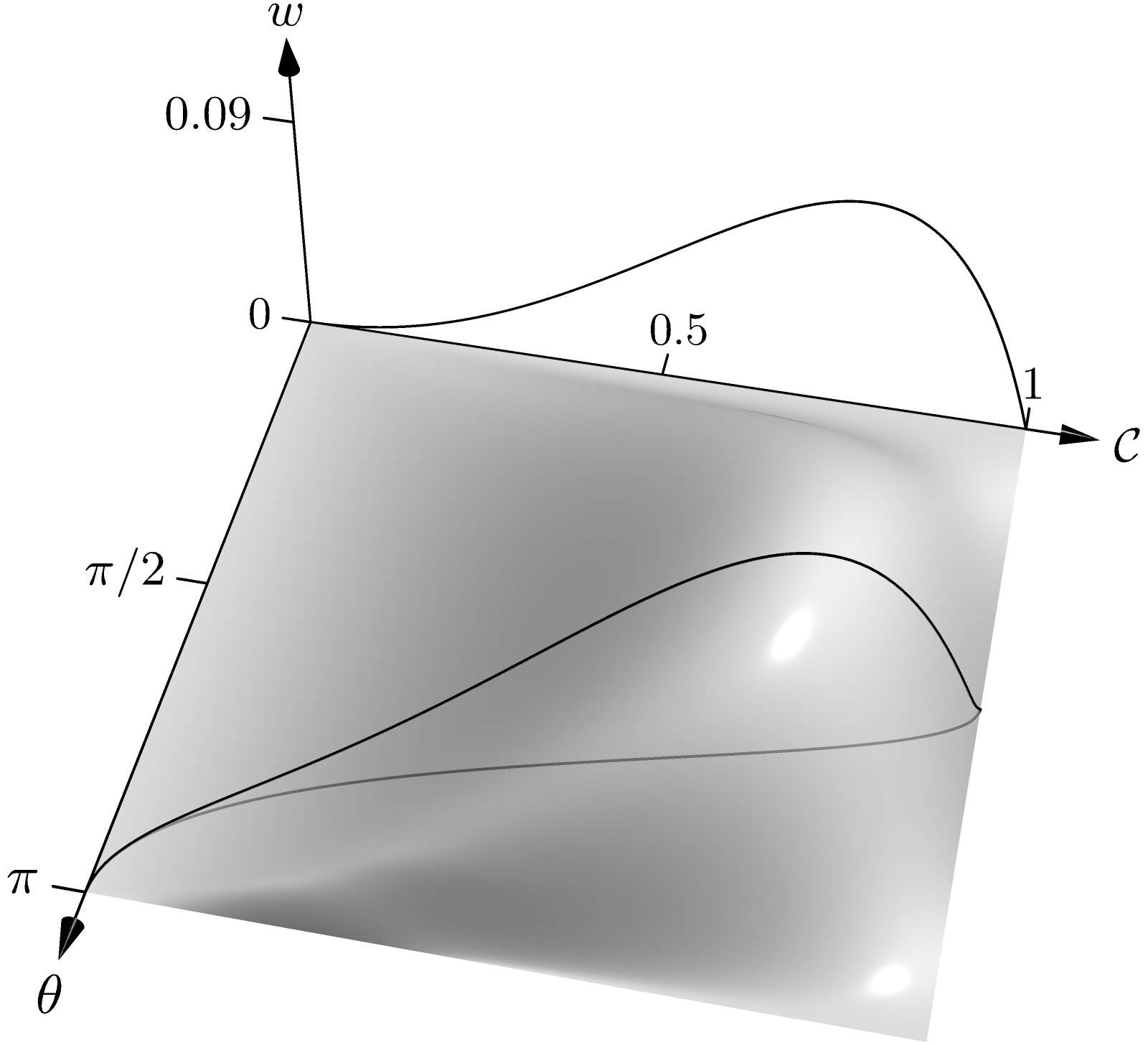
Therefore, we first analyze this result numerically. Figure 2 shows the probability $w$ as a function of the polar angle $\theta$ and the concurrence $\mathcal{C}$.

As a result, we obtain that the violation probability $w$ is vanishing for either separable states, that is $\mathcal{C}=0$, or maximally entangled states ($\mathcal{C}=1$). While the vanishing probability for $\mathcal{C}=0$ is expected, since entanglement is a key ingredient in the violation of the CHSH inequality, the case of a maximally entangled state is more of a surprise, as the CHSH inequality is in general maximally violated for a maximally entangled state. Hence, the vanishing probability must occur due to the additional constraints on the measurement vectors.

Moreover, the probability $w$ also vanishes if the polar angle of the measurement vector $\boldsymbol{q}$ is either $\theta=0$ or $\theta=\pi/2$. For these cases the vector $\boldsymbol{q}$ points along the positive or negative $z$ axis, respectively. This result is also not true for the general CHSH case, and thus must result from the additional constraints.

Furthermore, for any fixed concurrence $0<\mathcal{C}<1$ a unique angle $\theta$ exists, such that the probability $w$ is maximal. These values are indicated by the black line in Figure 2. For small concurrences the optimal angle is close to $\pi$, that is the optimal vector $\boldsymbol{q}$ points mostly along the negative $z$ axis. With increasing $\mathcal{C}$ the angle $\theta$ decreases monotonically towards $\pi/2$, that is the vector $\boldsymbol{q}$ moves towards the $x$-$y$ plane. For all concurrences the optimal vector $\boldsymbol{q}$ thus has a negative $z$ component.

In our numerical calculation of the probability $w$, we have seen that it is independent of the azimuthal angle $\phi$ of the vector $\boldsymbol{q}$. The probability is therefore symmetric under rotations around the $z$ axis. In this section we show this symmetry by proofing that all relevant vectors lie in a common plane, which contains the $z$ axis of our coordinate system.

In the expectation value $\mathcal{S}$, Equation 6, only combinations of a vector of the subsystem $A$ and a vector of the subsystem $B$ appear, while the correlation matrix $K$ specifies how vectors from different subsystems are multiplied to each other.

Instead of using the correlation matrix as a connection between the two subsystems, we directly apply the correlation matrix to the vectors of the subsystem $B$, defining the new vectors

and

These new vectors are no longer of unit length. Instead, their length depends on their orientation, since their components in the $x$ and $y$ direction are contracted by the factor $\mathcal{C}$.

The new vectors $\boldsymbol{s}_{K}$ and $\boldsymbol{t}_{K}$ directly multiply to the vectors $\boldsymbol{q}$ and $\boldsymbol{r}$ of the subsystem $A$ by the usual scalar product, that is we find

for the expectation value.

Our aim is to construct the vectors $\boldsymbol{q},\boldsymbol{r},\boldsymbol{s}_{K}$ and $\boldsymbol{t}_{K}$ geometrically. For this purpose we first show that these vectors lie in a common plane, defined by the vector

which is in general not parallel to the vector $\boldsymbol{q}$, and the Bloch vector $\boldsymbol{a}$.

From the definitions of $\boldsymbol{s}_{K}$ and $\boldsymbol{t}_{K}$, Equations 28 and 29, and of $\boldsymbol{s}$ and $\boldsymbol{t}$, Equations 25 and 24, the new vectors $\boldsymbol{s}_{K}$ and $\boldsymbol{t}_{K}$ are given by the explicit expressions

and

where we made use of the fact that the correlation matrix $K$ does not change the Bloch vector $\boldsymbol{a}$, since the latter points along the $z$ axis of our coordinate system.

In general the Bloch vector $\boldsymbol{a}$ is fixed, while the measurement vector $\boldsymbol{q}$ is our free parameter. For any arbitrary but fixed $\boldsymbol{q}$, it immediately follows form Equations 32 and 33, that $\boldsymbol{s}_{K}$ and $\boldsymbol{t}_{K}$ are in the plane $P$ spanned by the vectors $K^{2}\boldsymbol{q}$ and $\boldsymbol{a}$.

Furthermore, from Equations 26 and 29 it follows that the vector

is a linear combination of the two vectors $\boldsymbol{t}_{K}$ and $\boldsymbol{a}$. Therefore, the vector $\boldsymbol{r}$ also lies in the plane $P$.

Moreover, since the measurement vector $\boldsymbol{q}$ can be rewritten as

which directly follows form evaluating the right hand side, $\boldsymbol{q}$ is also a linear combination of $\boldsymbol{a}$ and $K^{2}\boldsymbol{q}$. The plane $P$ thus contains the vector $\boldsymbol{q}$.

Therefore all the four vectors appearing in Equation 30 lie in $P$ and we thus restrict our discussions and calculations for the remainder of our article to the plane $P$.

We finally note that the Bloch vector $\boldsymbol{a}$ is parallel to the $z$ axis of our coordinate system, and the plane $P$ thus contains the $z$ axis. Therefore, the second direction orthogonal on $z$ is a vector in the $x$-$y$ plane, which we denote by $x^{\prime}$. Hence, $P$ is the $x^{\prime}$-$z$ plane. From this form of $P$ it directly follows that the expectation value $\mathcal{S}$, Equation 30, is independent of the azimuthal angle $\phi$ of the vector $\boldsymbol{q}$, which is consistent with our results from the previous section.

The plane $P$ is only uniquely defined as long as the vectors $K^{2}\boldsymbol{q}$ and $\boldsymbol{a}$ are neither parallel nor either of them vanishes. We now examine the cases where this condition is not fulfilled.

The first case we consider is when $\boldsymbol{a}$ is vanishing. According to its definition, Equation 2, the Bloch vector only vanishes for $\mathcal{C}=1$, which furthermore implies $K=\diag(-1,1,1)$. Inserting these conditions into Equations 25, 24 and 26, we obtain $\boldsymbol{q}=\boldsymbol{s}_{K}=-\boldsymbol{t}_{K}=-\boldsymbol{r}$, and thus all relevant vectors point along the same line. From our expression of the expectation value, Equation 30, it immediately follows under these conditions that $\mathcal{S}=2$, and therefore $w=0$.

The second case we consider is that both $K^{2}\boldsymbol{q}$ and $\boldsymbol{a}$ are parallel, which corresponds to the vector $\boldsymbol{q}$ pointing along the $z$ axis of our coordinate system. It immediately follows from Equations 25, 24 and 26, that the three other vectors $\boldsymbol{r},\boldsymbol{s}_{K}$ and $\boldsymbol{t}_{K}$ also point along the $z$-axis of our coordinate system. By the same argument as for the case $\mathcal{C}=1$, it immediately follows, that $w=0$.

Finally, we consider the case of $K^{2}\boldsymbol{q}=0$, which is only achievable for $\mathcal{C}=0$. In this case the underlying state $\left|\Psi\right\rangle$ is separable. Since a separable state never violates the CHSH inequality, the violation probability $w$ is also vanishing.

Hence, the vectors $\boldsymbol{q},\boldsymbol{r},\boldsymbol{s}_{K}$ and $\boldsymbol{t}_{K}$ are either all located in a common well defined plane $P$ or they point along a single line. In the latter case, the probability $w$ always vanishes. Since we are only interested in obtaining a nonvanishing probability $w$, we restrict ourselves in the following to the case of all four vectors $\boldsymbol{q},\boldsymbol{r},\boldsymbol{s}_{K}$ and $\boldsymbol{t}_{K}$ lying in a common plane $P$.

We are now in the position to construct the four vectors $\boldsymbol{q}$, $\boldsymbol{r}$, $\boldsymbol{s}_{K}$ and $\boldsymbol{t}_{K}$ in the plane $P$ geometrically. This geometric interpretation is depicted in Figure 3.

We start with the vector $\boldsymbol{q}$, which is the only vector that can be chosen freely. Since $\boldsymbol{q}$ is a unit vector, it points from the origin of our new coordinate system to a unit circle.

The next vector we consider is the vector $\boldsymbol{s}_{K}$, which is given by Equation 32. When starting at the origin the vector $\boldsymbol{s}_{K}$ terminates in a point $S$ on an ellipse with semi major axis of unit length along the $z$ axis, and semi minor axis of length $\mathcal{C}$. Using the representation of the Bloch vector $\boldsymbol{a}$, Equation 2, the correlation matrix $K$, Equation 8, and the fact that $\boldsymbol{q}$ is a unit vector, we show in Appendix A that the vector

defines a line spanned by the support vector $-\boldsymbol{a}$ and the directional vector $\boldsymbol{q}$. Here, we introduced the abbreviation

with $q_{z}$ being the component of $\boldsymbol{q}$ along the $z$ axis.

We therefore geometrically construct the vector $\boldsymbol{s}_{K}$, and thus the point $S$, by going from the lower focal point $F_{l}$ in the direction of $\boldsymbol{q}$. The intersection with the ellipse constitutes the point $S$.

In an analogous way, we determine the point $T$ on the ellipse, which is defined by the vector $\boldsymbol{t}_{K}$ pointing from the origin to the ellipse. By using the definition of $\boldsymbol{t}$, Equation 24, as well as the Bloch vector $\boldsymbol{a}$, and the correlation matrix $K$, Equation 8, we demonstrate in Appendix A that the vector

where we introduced the abbreviation

is constructed by going from the lower focal point $F_{l}$ in the direction $-\boldsymbol{q}$ to the ellipse.

Our construction directly shows that, as a consequence of the additional constraints, Equations 25 and 24, the line $ST$, which also defines the vector $\boldsymbol{s}_{K}-\boldsymbol{t}_{K}$, intersects the $z$ axis in the focal point $F_{l}$ of the ellipse.

From the vectors $\boldsymbol{s}_{K}$ and $\boldsymbol{t}_{K}$ we construct the vectors $-\boldsymbol{s}_{K}$ and $-\boldsymbol{t}_{K}$, which point from the origin to the points $\bar{S}$ and $\bar{T}$, respectively, on the ellipse. Due to symmetry, the line $\bar{S}\bar{T}$, which also determines to the vector $\boldsymbol{s}_{K}-\boldsymbol{t}_{K}$, intersects the $z$ axis in the upper focal point $F_{u}$.

The only vector left is the vector $\boldsymbol{r}$. In Appendix A we derive that this vector is given by the linear combination

of the measurement vector $\boldsymbol{q}$ and the Bloch vector $\boldsymbol{a}$. This expression shows that the vector $\boldsymbol{r}$ can be constructed by going from the origin of our coordinate system to the end point of the vector $\boldsymbol{q}$ and then along the direction $-(\boldsymbol{q}+\boldsymbol{a})$, which is through the focal point $F_{l}$, until one again intersects the unit circle. This intersection is then the end point of the vector $\boldsymbol{r}$. As a consequence of this construction, it is obvious that the line between the two end points of the vectors $\boldsymbol{q}$ and $\boldsymbol{r}$ on the unit circle includes the focal point $F_{l}$.

This behaviour is similar to the construction of the points $S$ and $T$, where the line $ST$ also includes the same focal point $F_{l}$.

We furthermore notice, that the vector $\boldsymbol{r}$ is by its definition, Equation 26, parallel to the vector $\boldsymbol{t}_{K}-\boldsymbol{a}$, and therefore the line $\bar{T}F_{l}$ between the point $\bar{T}$, defined by the vector $-\boldsymbol{t}_{K}$, on the ellipse and the focal point $F_{l}$.

We now utilize the geometrical picture of the vectors $\boldsymbol{q}$, $\boldsymbol{r}$, $\boldsymbol{s}_{K}$ and $\boldsymbol{t}_{K}$ to find a geometrical interpretation of the violation probability $w$. We start by determining the expectation value $\mathcal{S}$ in our geometrical picture. We then use this result to relate the probability $w$ to the length difference in a triangle.

The expectation value $\mathcal{S}$, Equation 6, consist of the two terms $\boldsymbol{q}\cdot(\boldsymbol{s}_{K}-\boldsymbol{t}_{K})$ and $\boldsymbol{r}\cdot(\boldsymbol{s}_{K}+\boldsymbol{t}_{K})$.

The first scalar product

is the length of the line segment $\bar{S}\bar{T}$, since $\boldsymbol{q}$ is parallel to $\boldsymbol{s}_{K}-\boldsymbol{t}_{K}$.

The measurement vector $\boldsymbol{r}$ is in general not parallel to $\boldsymbol{s}_{K}+\boldsymbol{t}_{K}$. Thus, the second scalar product

is the distance between the points $\bar{T}$ and $R$, where the latter is defined by the parallel projection of $\boldsymbol{s}_{K}+\boldsymbol{t}_{K}$ on the vector $\boldsymbol{r}$.

From Figure 4(a) and the focal point property of the ellipse, we find the relation

where $\lambda$ is the signed length of the line segment $|RF_{l}|$ between the point $R$ and the lower focal point $F_{l}$. Note, that $\lambda$ is defined positive if $R$ is between $\bar{T}$ and $F_{l}$, and negative otherwise.

Inserting the expressions for the two scalar products, Equations 41 and 42, together with the relation between the different lengths, Equation 43, into the expectation value $\mathcal{S}$, Equation 30, we find

This result is understood geometrically from Figure 4. The expectation value is the distance from the point $\bar{S}$ via the point $\bar{T}$ to the point $R$. If we instead of $R$ went to the point $F_{l}$ this distance would be $2+\xi$, due to the focal point property. Since we only go to $R$, we have to subtract the additional length $\lambda$. We note, that $R$ can be in principle be further away from $\bar{T}$ than $F_{l}$. To include this effect, $\lambda$ is negative in this case.

When we insert this result into Equation 20, we find that the violation probability

is proportional to the difference between the two lengths $\xi$ and $\lambda$. Geometrically, the violation probability manifests itself as the difference between the hypothenuse and the leg of a right triangle. This interpretation is depicted in Figure 4(b).

In Appendix C, we further discuss the geometric interpretation of $w$ and derive the expression

which only depends on the concurrence $\mathcal{C}$ and the distance $\tau$ between the point $\bar{T}$ and the focal point $F_{u}$.

We start by maximizing the probability $w$, Equation 46, for an arbitrary but fixed concurrence $\mathcal{C}$ over all possible lengths $\tau$ by calculating the derivative

and determining its roots. Straightforward algebra shows, that the roots are given by

and since $\tau$ represents a length, only the positive solution

allows us to optimize the probability $w$.

Inserting the optimal length $\tau_{\mathrm{opt}}$, Equation 49, into the expression of $w$, Equation 46, we obtain

as the optimal violation probability in the Hardy scenario, as a function of the concurrence $\mathcal{C}$.

We now consider two special cases of the optimal violation probability $w_{\mathrm{opt}}$. The first case is small concurrences, that is when the common bipartite state is nearly separable. The second case we consider is the case of $\mathcal{C}\lesssim 1$, that is for almost maximally entangled states.

For small concurrences, we expand the optimal expectation value, given by Equation 50, into the Taylor series

at $\mathcal{C}=0$. Thus, for small entanglement, the expectation value and thus the probability $w$ grows quadratically with the concurrence. This behavior is similar to the optimal expectation value $\mathcal{S}_{\mathrm{opt}}=2\sqrt{1-\mathcal{C}^{2}}$ for the CHSH scenario, which also grows quadratically in the concurrences for small $\mathcal{C}$. In fact, the violation probability $w_{\mathrm{opt}}$ of the Hardy scenario only differs in order $\mathcal{O}(\mathcal{C}^{5})$ from its corresponding value in the CHSH scenario. Therefore, for small concurrences $\mathcal{C}$ the additional constraints Equations 25, 24 and 26 have a negligible effect on the achievable expectation value $\mathcal{S}_{\mathrm{opt}}$, and thus on the optimal violation probability $w_{\mathrm{opt}}$.

For $\mathcal{C}\lesssim 1$, we expand Equation 50 around $\epsilon=1-\mathcal{C}$, and find

which decreases linearly with the concurrence when $\mathcal{C}$ goes to $1$. For maximally entangled states, that is $\mathcal{C}=1$, the violation probability $w$ vanishes. This behavior differs completely from the CHSH scenario, where the optimal expectation value $\mathcal{S}_{\mathrm{opt}}$ obtains its maximal value for the maximally entangled state, that is for $\mathcal{C}=1$.

Since the probability $w$ vanishes for both extreme cases $\mathcal{C}=0$ and $\mathcal{C}=1$ but is non vanishing for $0<\mathcal{C}<1$, an optimal concurrence $\mathcal{C}_{\mathrm{opt}}$ must exist, which maximizes the optimal probability $w_{\mathrm{opt}}(\mathcal{C})$, Equation 50.

By differentiating $w_{\mathrm{opt}}(\mathcal{C})$, Equation 50, and determining the root of the resulting expression, the optimal concurrence reads

When we insert the optimal concurrence $\mathcal{C}_{\mathrm{opt}}$ into the optimal length of $\tau_{\mathrm{opt}}$, Equation 49, and

we find that their ratio

is the golden ratio $\Phi$. Due to the relation

which is valid for all concurrences $\mathcal{C}$, the ratio between the lengths $\tau$ and $2-\tau$ is also determined by the golden ratio.

From the definition of the golden ration, the relation

follows directly. As a consequence, by comparing Equation 56 with Equation 57, we find that for the optimal concurrence, we have

that is the distance between the points $\bar{S}$ and $\bar{T}$, which are defined by the end points of the vectors $-\boldsymbol{s}_{K}$ and $-\boldsymbol{t}_{K}$ on the ellipse, is equal to the distance between the point $\bar{T}$ and the lower focal point of the ellipse $F_{l}$.

In order to determine the optimal vectors, we first parameterize the vector

by the polar angle $\theta$ between the vector $\boldsymbol{q}$ and the $z$ axis.

Inserting this representation of the vector $\boldsymbol{q}$ back into the definition of $\tau$, Equation 39, and setting the result equal to the optimal length $\tau_{\mathrm{opt}}$, Equation 49, we determine the optimal angle

as a function of the concurrence $\mathcal{C}$. This function is depicted in Figure 5.

The optimal angle is therefore always in the interval $\pi/2$ to $\pi$ and hence the vector $\boldsymbol{q}$ lives in the lower half of the Bloch sphere. For $\mathcal{C}\to 0$ the optimal angle is close to $\pi$, that is the vector $\boldsymbol{q}$ points mostly along the negative $z$ axis. With increasing concurrence $\mathcal{C}$ the optimal angle decreases. For $\mathcal{C}\to 1$ the deviation from $\boldsymbol{q}$ points mostly along the $x^{\prime}$ axis ($\theta=\pi/2$).

Indeed, when we insert Equation 60 into Equation 59, we obtain

which when we also consider the azimuthal angle $\phi$ leads to the three dimensional measurement vector

When we choose $\phi=0$ that is the vector $\boldsymbol{q}$ in the $x$-$z$ plane, inserting $\boldsymbol{q}_{\mathrm{opt}}$, Equation 62, into the definition of $\boldsymbol{t}$, Equation 24, leads to

and the two optimal measurement vectors point along the same direction in their respective coordinate system. By inserting this result into the expression for $\boldsymbol{s}$, Equation 25, and comparing it with the expression for $\boldsymbol{r}$, Equation 26, we furthermore find

As a consequence, the optimal measurement setting is to choose the measurements symmetrically on both subsystems $A$ and $B$ of the bipartite state.

We note that these measurement settings are assumptions explicitly made by Hardy in his original article Hardy 1993. Hence allowing $\boldsymbol{q}$ and $\boldsymbol{t}$ to be non equal measurement directions does not improve the probability $w$ to violate the nonlocality assumption.

In the previous sections we have determined the optimal measurements. We now ask the questions of how important the exact choice of these measurement settings is in obtaining a significant violation probability. For this purpose, we investigate the case of fixing the measurement vector $\boldsymbol{q}$ to point along the $x^{\prime}$ axis of our coordinate system. This situation has the advantage that we do not have to adjust this measurement operator to the underlying state, but only the other three measurements $\boldsymbol{r},\boldsymbol{s}$ and $\boldsymbol{t}$, where the latter two have the same $z$ component and differ in the $x^{\prime}$ component only in the sign.

When $\boldsymbol{q}$ points along the $x^{\prime}$ axis, it follows from the definition of the length $\tau$, Equation 38, that $\tau=\mathcal{C}^{2}$, which by inserting into the expression for the violation probability, Equation 46, leads to

In Figure 6, we depict this function and compare it to the optimal measurement strategy for the Hardy scenario. For small concurrences, that is in the limit $\mathcal{C}\ll 1$, a Taylor expansion of Equation 65 gives

and thus the expectation value grows quadratically in the concurrence. Compared to the Taylor expansion for small concurrences for the optimal violation probability $w_{\mathrm{opt}}$, Equation 51, the approximation $w_{r}$ only differs up to fourth order in $\mathcal{C}$, and thus for small concurrences the differences in the violation probability for the optimal and the case, where $\boldsymbol{q}$ points along the $x^{\prime}$ axis, are negligible.

This result seems quite surprising, since in the previous section, we have seen that the optimal angle for small concurrences is close to $\theta=\pi$. Thus, for small concurrences the choice of the measurement vector $\boldsymbol{q}$ is not the relevant parameter for increasing the achievable violation probability $w$.

For $\mathcal{C}\lesssim 1$, we perform a Taylor expansion of the violation probability, Equation 65, for the small parameter $\epsilon=1-\mathcal{C}$

at $\epsilon=0$. The expectation value thus grows linearly with $\epsilon$, corresponding to a linear decay towards $2$ for $\mathcal{C}\to 1$. When we compare this expansion, Equation 67, to the Taylor series at $\mathcal{C}=1$ of the optimal expectation value, Equation 52, we find that they agree in first order and differ only slightly in the second order of $\epsilon$. Thus, for $\mathcal{C}\lesssim 1$ the choice of $\boldsymbol{q}$ pointing along the $x^{\prime}$ axis provides a good approximation for the optimal measurement. This result is no surprise, since the optimal angle $\theta_{\mathrm{opt}}$, Equation 60, converges to $\pi/2$, when $\mathcal{C}$ goes to $1$.

The difference $\Delta w=w_{\mathrm{opt}}-w$ between the optimal violation probability and $\boldsymbol{q}$ pointing along $x^{\prime}$ is largest for $\mathcal{C}\approx 0.75$ where the violation probability is decreased by $\Delta w\approx 0.44\%$ from the optimal probability.

We start by discussing the case of a single constraint applied to the measurement vectors. We first show that all three constraints lead to the same optimal expectation value $\mathcal{S}_{\mathrm{opt}}$ and are therefore equivalent.

For this purpose, we note that relabeling the subsystems $A$ and $B$, as well as the respective measurements does not change the physical system. Thus, by exchanging the vectors $\boldsymbol{q}$ and $\boldsymbol{t}$ as well as the vectors $\boldsymbol{r}$ and $\boldsymbol{s}$, the constraint between the vectors $\boldsymbol{q}$ and $\boldsymbol{s}$, Equation 16, becomes the constraint between $\boldsymbol{t}$ and $\boldsymbol{r}$, Equation 17, and vice versa. If we only restrict the vector $\boldsymbol{s}$ by Equation 16 while we choose the vectors $\boldsymbol{q}$, $\boldsymbol{r}$ and $\boldsymbol{t}$ freely, this corresponds to the same situation as restricting $\boldsymbol{r}$ by Equation 17, while choosing $\boldsymbol{q}$, $\boldsymbol{s}$ and $\boldsymbol{t}$ independently.

Furthermore, by interchanging the vector $\boldsymbol{q}$ with $-\boldsymbol{q}$, the restriction between $\boldsymbol{q}$ and $\boldsymbol{t}$, Equation 15, is equivalent to the connection between the vectors $\boldsymbol{q}$ and $\boldsymbol{s}$, Equation 16. Thus, the case of $\boldsymbol{t}$ being determined by $\boldsymbol{q}$, while the other measurement vectors $\boldsymbol{q}$, $\boldsymbol{s}$ and $\boldsymbol{r}$ are chosen freely, is equivalent to the case of only $\boldsymbol{s}$ being restricted by $\boldsymbol{q}$, while $\boldsymbol{q}$, $\boldsymbol{t}$ and $\boldsymbol{r}$ are chosen independently. As a result, all three conditions lead to the same optimal expectation value $\mathcal{S}_{\mathrm{opt}}$.

Unfortunately, the optimization for only a single constraint is rather difficult to perform analytically, and we are therefore content with a numerical optimization. The optimal expectation value is shown by the red curve in Figure 7. In this picture, we compare it to the CHSH case (black curve) and the Hardy scenario (blue curve).

For small concurrences $\mathcal{C}$, the optimal expectation value is similar to both the behavior of the CHSH inequality and the Hardy scenario. This result is no surprise, since we have already demonstrated in the previous section that the Hardy scenario and the CHSH inequality lead to almost the same behavior for small concurrences, and a single condition can neither lead to a result better than the CHSH case, nor worse than the Hardy scenario.

For medium concurrences, that is $0.5\lesssim\mathcal{C}\lesssim 0.8$, the single constraint case is still similar to the CHSH case, but starts to deviate clearly from the Hardy constraints. For large concurrences, there exists a maximum of the optimal expectation value $\mathcal{S}_{\mathrm{opt}}\approx 2.64$ at $\mathcal{C}\approx 0.95$, while for larger concurrences the optimal expectation value decreases down to $\mathcal{S}_{\mathrm{opt}}=2.5$ for $\mathcal{C}=1$.

Hence, a single constraint is sufficient to obtain the optimal expectation value $\mathcal{S}_{\mathrm{opt}}$ for a non maximally entangled state ($\mathcal{C}<1$). The associated entanglement of the underlying state is larger than for the Hardy scenario. In contrast to the Hardy scenario, the optimal expectation value does not decrease towards $\mathcal{S}_{\mathrm{opt}}=2$, that is the classical boundary, for $\mathcal{C}\to 1$. Thus, it is always possible to achieve a violation of the CHSH inequality with a single constraint for maximally entangled states.

We now consider the case of two restrictions. We start by lifting the restriction between the measurement vectors $\boldsymbol{r}$ and $\boldsymbol{t}$, Equation 17, compared to the Hardy scenario. Thus, the vectors $\boldsymbol{s}$ and $\boldsymbol{t}$ are still defined by the choice of $\boldsymbol{q}$, while the vector $\boldsymbol{r}$ is chosen independently.

In Section III we demonstrated that from the two constraints, Equations 16 and 15, on the vectors $\boldsymbol{s}_{K}$ and $\boldsymbol{t}_{K}$, it follows that the parallelogram defined by the points $S,T,\bar{S}$ and $\bar{T}$ intersects the $z$ axis in the focal points $F_{u}$ and $F_{l}$ of the ellipse.

Furthermore, we have seen that the measurement vector $\boldsymbol{q}$ is parallel to the vector $\boldsymbol{s}_{K}-\boldsymbol{t}_{K}$. The other measurement vector $\boldsymbol{r}$ on the subsystem $A$ is not constraint anymore, and we choose it parallel to the vector $\boldsymbol{s}_{K}+\boldsymbol{t}_{K}$. Then, maximizing the expectation value $\mathcal{S}$ corresponds to maximizing the perimeter of a parallelogram enclosed by an ellipse which goes through the focal points of the ellipse.

From numerical optimization we find, that the optimal parallelogram that fulfills these conditions is the rectangle whose sides are parallel to the $x^{\prime}$ and $z$ axis. In this case, it is straightforward to see that the side parallel to the $z$ axis has length $2\sqrt{1-\mathcal{C}^{2}}$, while the side parallel to the $x^{\prime}$ axis is of length $2\mathcal{C}^{2}$. The rectangle therefore has a perimeter of $4(\mathcal{C}^{2}+\sqrt{1-\mathcal{C}^{2}})$.

Therefore, the optimal expectation value is given by

and consists of an increasing and a decreasing term with the concurrence $\mathcal{C}$.

In Figure 7 we depict the expectation value $\mathcal{S}$ under these constraints (orange curve), alongside the expectation values $\mathcal{S}$ for the CHSH case (black curve), that is without any constraints, and the Hardy scenario (blue curve).

The expectation value given by Equation 68 is not monotonic in $\mathcal{C}$. Instead for both $\mathcal{C}=0$ and $\mathcal{C}=1$ the maximum $\mathcal{S}_{\mathrm{opt}}=2$ cannot violate the CHSH inequality, while for all concurrences in between the maximum is strictly above $2$, and a violation is possible.

The decrease of $\mathcal{S}_{\mathrm{opt}}$ for $\mathcal{C}\to 1$ can be understood geometrically, which is depicted in Figure 8, and is a consequence of demanding the parallelogram to go through the focal points. Increasing $\mathcal{C}$ increases the semi minor axis of the ellipse, and allows the side of the rectangle parallel to the semi minor axis to increase. At the same time, the focal points move in closer towards the center of the ellipse, decreasing the length of the sides parallel to the semi major axis. In the limit of approaching a maximally entangled state $\left|\Psi\right\rangle$, the focal points collapse onto the origin of the ellipse (which is distorted to a circle) and the rectangle collapse onto a line along the $x$ axis of our coordinate system.

Finally, we note that for the concurrence $\mathcal{C}=\sqrt{3}/2$ the violation of the CHSH inequality is maximal, at which the expectation value, Equation 68, assumes the value $\mathcal{S}_{\mathrm{opt}}=2.5$. For larger concurrences this value rapidly decreases towards the classical bound $\mathcal{S}_{\mathrm{opt}}=2$.

We conclude the situation of having two measurement vectors depending on a single measurement vector by considering the case, where only constraints between the vectors $\boldsymbol{q}$, $\boldsymbol{r}$ and $\boldsymbol{t}$, Equations 15 and 17 are present, while we lift the constraint between $\boldsymbol{q}$ and $\boldsymbol{s}$, Equation 16. When we interchange the vectors $\boldsymbol{q}$ with $\boldsymbol{t}$ and $\boldsymbol{r}$ with $\boldsymbol{s}$ in the conditions, Equations 17 and 15, they are identical to the conditions discussed above, Equations 16 and 15. Therefore, the two cases are equivalent, and we obtain the same result for the optimal expectation value $\mathcal{S}_{\mathrm{opt}}$.

In contrast to the two previous cases, the case of two constraints on $\boldsymbol{s}$ and $\boldsymbol{r}$, Equations 16 and 17, is different and cannot be mapped to the other cases of two constraints. We again optimize the expectation value $\mathcal{S}_{\mathrm{opt}}$ under these constraints numerically, and depict the result by the green curve in Figure 7.

As a result, the two constraints Equations 16 and 17 lead to a reduced optimal expectation value $\mathcal{S}_{\mathrm{opt}}$, compared to the case of applying the constraints, Equations 16 and 15 or Equations 15 and 17. For small concurrences the behavior is similar to the other cases, with various constraints. For large concurrences, the optimal expectation value again decreases towards the classical limit $\mathcal{S}=2$ for $\mathcal{C}\to 1$. For $\mathcal{C}\approx 0.84$ we obtain the maximal expectation value $\mathcal{S}_{\mathrm{opt}}\approx 2.43$. Thus, the optimal concurrence is larger than for the Hardy constraints, $\mathcal{C}_{\mathrm{opt}}=3-\sqrt{5}$, but lower than when we apply the other two constraints simultaneously.

We therefore conclude that two out of the three constraints for the Hardy scenario always lead to the decay of the optimal expectation value $\mathcal{S}_{\mathrm{opt}}$ to the classical regime for maximally entangled states. The main differences between the results for these different conditions is found in the regime $0.5\lesssim\mathcal{C}\lesssim 0.9$, where the achievable expectation value crucially depends on the underlying constraints.

References

- Bell (1964) J. S. Bell, On the Einstein Podolsky Rosen paradox, Physics 1, 195 (1964).
- Brunner et al. (2014) N. Brunner, D. Cavalcanti, S. Pironio, V. Scarani, and S. Wehner, Bell nonlocality, Rev. Mod. Phys. 86, 419 (2014).
- Freedman and Clauser (1972) S. J. Freedman and J. F. Clauser, Experimental test of local hidden-variable theories, Phys. Rev. Lett. 28, 938 (1972).
- Fry and Thompson (1976) E. S. Fry and R. C. Thompson, Experimental test of local hidden-variable theories, Phys. Rev. Lett. 37, 465 (1976).
- Aspect et al. (1982a) A. Aspect, P. Grangier, and G. Roger, Experimental realization of Einstein-Podolsky-Rosen-Bohm Gedankenexperiment: A new violation of Bell’s inequalities, Phys. Rev. Lett. 49, 91 (1982a).
- Aspect et al. (1982b) A. Aspect, J. Dalibard, and G. Roger, Experimental test of Bell's inequalities using time- varying analyzers, Phys. Rev. Lett. 49, 1804 (1982b).
- Weihs et al. (1998) G. Weihs, T. Jennewein, C. Simon, H. Weinfurter, and A. Zeilinger, Violation of Bell's inequality under strict Einstein locality conditions, Phys. Rev. Lett. 81, 5039 (1998).
- Hensen et al. (2015) B. Hensen, H. Bernien, A. E. Dréau, A. Reiserer, N. Kalb, M. S. Blok, J. Ruitenberg, R. F. L. Vermeulen, R. N. Schouten, C. Abellàn, et al., Loophole-free Bell inequality violation using electron spins separated by 1.3 kilometres, Nature 526, 682 (2015).
- Giustina et al. (2015) M. Giustina, M. A. Versteegh, S. Wengerowsky, J. Handsteiner, A. Hochrainer, K. Phelan, F. Steinlechner, J. Kofler, J.-Å. Larsson, C. Abellán, et al., Significant-loophole-free test of Bell’s theorem with entangled photons, Phys. Rev. Lett. 115, 250401 (2015).
- Shalm et al. (2015) L. K. Shalm, E. Meyer-Scott, B. G. Christensen, P. Bierhorst, M. A. Wayne, M. J. Stevens, T. Gerrits, S. Glancy, D. R. Hamel, M. S. Allman, et al., Strong loophole-free test of local realism, Phys. Rev. Lett. 115, 250402 (2015).
- Clauser et al. (1969) J. F. Clauser, M. A. Horne, A. Shimony, and R. A. Holt, Proposed experiment to test local hidden-variable theories, Phys. Rev. Lett. 23, 880 (1969).
- Hardy (1993) L. Hardy, Nonlocality for two particles without inequalities for almost all entangled states, Phys. Rev. Lett. 71, 1665 (1993).
- Kwiat and Hardy (2000) P. G. Kwiat and L. Hardy, The mystery of the quantum cakes, Am. J. Phys. 68, 33 (2000).
- Greenberger et al. (1990) D. M. Greenberger, M. A. Horne, A. Shimony, and A. Zeilinger, Bell’s theorem without inequalities, Am. J. Phys. 58, 1131 (1990).
- Cerf et al. (2002) N. J. Cerf, S. Massar, and S. Pironio, Greenberger-Horne-Zeilinger paradoxes for many qudits, Phys. Rev. Lett. 89, 080402 (2002).
- János A. Bergou (2013) M. H. János A. Bergou, Introduction to the Theory of Quantum Information Processing (SPRINGER NATURE, 2013).
- Wootters (1998) W. K. Wootters, Entanglement of formation of an arbitrary state of two qubits, Phys. Rev. Lett. 80, 2245 (1998).
- Rungta et al. (2001) P. Rungta, V. Bužek, C. M. Caves, M. Hillery, and G. J. Milburn, Universal state inversion and concurrence in arbitrary dimensions, Phys. Rev. A 64, 042315 (2001).
- Cirel'son (1980) B. S. Cirel'son, Quantum generalizations of Bell's inequality, Lett. Math. Phys. 4, 93 (1980).
- Tsirel'son (1987) B. S. Tsirel'son, Quantum analogues of the Bell inequalities. The case of two spatially separated domains, J. Math. Sci. 36, 557 (1987).
- Gisin (1991) N. Gisin, Bell's inequality holds for all non-product states, Phys. Lett. A 154, 201 (1991).
- Seiler et al. (2021) J. Seiler, T. Strohm, and W. P. Schleich, Geometric interpretation of the Clauser-Horne-Shimony-Holt inequality of nonmaximally entangled states, Phys. Rev. A 104, 032218 (2021).