Computer Generated Holograms (CGH), also known as Diffractive Null Correctors (DNC) or Diffractive Null Lenses (DNL) are used to convert a given input wavefront to a given output wavefront. Interferometric optical metrology of an aspheric surface requires converting a spherical wavefront to the nonspherical wavefront correponding to the exact shape of the surface. CGHs have a long history, see Reference (1) and are currently used widely in optical fabrication since many modern optical systems have one or more asphere surfaces in them, see References (2-5). As might be guessed from the name, CGHs are usually designed on a computer using some type of optimization algorithm. Here we show that the CGH design for a given asphere can be derived analytically using the grating equation. As described below, in some cases, the analytical solution must be evaluated numerically to invert one of the relationships since the closed form analytical solution can be very complex. This solution also can be found analytically by iteration, depending on the desired accuracy.

My guess is the discussion below is common knowledge and that most everyone already knows it and/or has worked it out for themselves. In any case here is my derivation of the equation for the design of a CGH.

The purpose of a Computer Generated Hologram (CGH), some times referred to as a Diffractive Null Corrector, is to covert an outgoing spherical wavefront into a wavefront which, when propagated to the surface of an asphere, is a perfect match to the asphere surface and hence is reflected directly back onto itself. In terms of geometrical optics this means the CGH diverts the rays in an outgoing spherical bundle so that every ray is incident on the asphere surface exactly along the local unit normal to the asphere surface at that point. In this way every ray in the bundle is reflected directly back onto itself and retraces it’s way back through the CGH to become part of an incoming spherical bundle of rays. This is illustrated in Figure 1 below.

Under the assumption that the asphere is radially symmetric we can use 2D transverse $\rho$ and longitudinal $z$ coordinates. The values of $\rho$ and $z$ are measured from the vertex of the asphere whose shape is given, as shown in Figure 1, by

$$z=A\left(\rho\right)$$

With the CGH located a distance $L$ along the optic axis from the vertex of the asphere, the surface of a spherical wavefront $S\left(\rho\right)$ of radius $R$ with its vertex on the optic axis at the CGH, see Figure 2, is given by

$$z=S\left(\rho\right)+L=R-\sqrt{R^{2}-\rho^{2}}+L$$

Although the CGH can be any pattern in principle, it nominally is a circular grating with a variable period as a function of radius. The local period $P\left(\rho\right)$ of the CGH grating pattern constitutes the design of the CGH. The local period is chosen so that it meets the criteria discussed above, i.e., it converts every ray in an outgoing spherical bundle of rays into a ray that is incident on the apshere surface along the local unit normal to the surface at the point of intersection. Given this criterion the design of the CGH, i.e, the variable grating period $P\left(\rho\right)$ can be determined by using the grating equation.

There are several issues that must be considered when designing a CGH. First, although it is possible in principle to compensate for the effect of the CGH being placed where it intersects the asphere caustic, it is much easier and more straightforward to place the CGH outside the region of the asphere caustic. Below we show how to calculate the caustic position in space and what the constraint is on the placement of the CGH to avoid having it intersect the caustic. Second, the design should make the CGH as easily manufacturable as possible, i.e., the size of the CGH should be reasonable and the smallest period or feature size in the grating pattern, should be easily printable. Both the minimum feature size and the overall size of the CGH are dependent on the interferometer configuration and the placement of the CGH in the interferometer. But reasonable sizes for the CGH are on the order of a few cm to a few 10’s of cm. To avoid having to account for Maxwell electromagnetic effects, the minimum feature size in the CGH should be greater than around 4 or 5 times the wavelength of the light used by the interferometer which nominally will be 632.8 nm. Third, the CGH will generally be a binary structure on glass forming either a ”phase grating” or an ”amplitude grating”. It follows from symmetry that binary, i.e, square wave shaped, grating structures must have exactly the same diffraction efficiency in the $+n$ and $-n$ diffraction orders at normal incidence. For grating periods that are large compared to the wavelength $\lambda$ of the light, the $+n$ and $-n$ diffraction order efficiencies stay very much the same even away from normal incidence. What this means is that even if the signal we want to detect is just in the $+n$ order, the CGH will be generating a roughly equal amount of $-n$ diffraction order along with other diffraction orders which we don’t want to detect. We can place an aperture near the focus of the return spherical wave blur circle which can significantly reduce, but not completely eliminate the effects of the unwanted orders. On the other hand a “carrier” frequency can be added to the CGH to divert the nonzero diffraction orders off-axis or away from the origin. Which approach should be used requires carefully evaluating the effect of the remaining contribution from the unwanted orders on the error budget for the CGH, along with the effect of fabrication and alignment tolerances.

Finally, one might expect the best overall CGH design involves having it, on average, deviate the rays by the minimal possible amount but this can lead to what might best be termed the ”diffraction order swap” issue. Consider a radially symmetric asphere and radially symmetric CGH perfectly aligned with one another. The ray on the optic axis is undeviated and this implies the grating period at the center of CGH should be infinite for any non-zero diffraction order. Obviously you cannot have an infinite period on a finite size CGH. But based on the spatial resolution of the interferometer, the actual CGH period only needs to be the local spatial average of the ”exact” design determined using the grating equation. The spatial average reduces the infinite period down to a finite value. The size of the spatial averaging region should correspond, for a well designed, built and aligned interferometer, to the interferometer spatial resolution which is the interferometer pixel size mapped to the CGH. If the ray deviation at some other position on the CGH surface is also zero, it also nominally requires an infnite period at that position and most likely, considered radially, the desired diffraction orders on opposite sides of this region will have opposite signs, e.g., we want the +1 order on one side and $-$1 order on the other side. As stated above an aperture placed close to the focal plane of the spherical wavefront will automatically filter out anything that is not close to the desired spherical wavefront.

Also note that the CGH design, which is given by the grating period as a function of position, and the fact that it will be spatially averaged mitigates to greater or lesser extent the difference between the intensity of diffracted orders from so called phase and amplitude gratings. A perfect 0/$\pi$ phase grating is expected to have 0 intensity in the zeroth diffraction order, but this is strictly true only for an infinite phase grating. Any finite size phase grating depending on detector area, distance from the grating, intervening optics will generally have a non-zero intensity in the detected ”zeroth diffraction order”.

Figure 2 shows the return path of one of the rays starting at the surface of the asphere. We will determine the local period of the CGH by applying the grating equation to the return path. If the return rays precisely retrace the outgoing path then the period determined from the outgoing rays is identical.

NOTE: The spherical wavefront is, by definition, radially symmetric about the optic axis. We will assume the asphere is symmetric about the optic axis as well and hence we can consider the CGH to be symmetric about the optic axis. This is not necessary, but it is useful for a first analysis.

NOTATION: We will use vector notation in which $\hat{\rho}$ and $\hat{z}$ are unit vectors in the $\rho$ and $z$ directions, respectively.

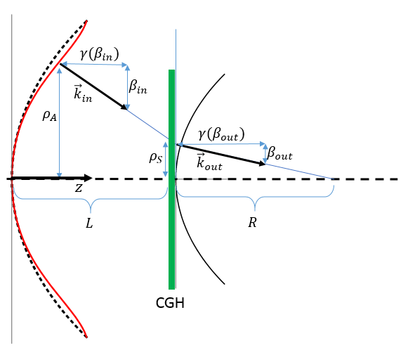
The local period $P$ of the CGH at position $\rho_{S},$ which we denote as $P\left(\rho_{S}\right)$ must be such that $\vec{k}_{in}$ in Figure 2 is converted to $\vec{k}_{out}$ where $\vec{k}_{out}$ corresponds to a return ray of the spherical bundle and, at the point where it intersects the asphere $\vec{k}_{in}$ is perpendicular to the surface of the asphere. For a return spherical wavefront of radius $R$ as shown in the Figure 2 $\vec{k}_{out}$ is given by

$$\vec{k}_{out}=\beta_{out}\hat{\rho}+\gamma\left(\beta_{out}\right)\hat{z}$$

with

$$\gamma\left(\beta_{out}\right)=\sqrt{k^{2}-\beta_{out}^{~2}}$$

where $k=2\pi/\lambda.$ In terms of the propagation angle $\phi_{out}$ of $\vec{k}_{out}$, measured with respect to the $z$ axis,

	$\displaystyle\beta_{out}$	$\displaystyle=-k\sin\left(\phi_{out}\right)=-k\frac{\rho_{S}}{\sqrt{R^{2}-\rho_{S}^{2}}}$
	$\displaystyle\gamma\left(\beta_{out}\right)$	$\displaystyle=k\cos\left(\phi_{out}\right)=\sqrt{k^{2}-\beta_{in}^{~2}}=k\sqrt{1-\left(\frac{\rho_{S}}{R^{2}+\rho_{S}^{2}}\right)^{2}}=,k\frac{R}{\sqrt{R^{2}+\rho_{S}^{2}}}$

The minus sign for $\beta_{out}$ simply indicates that $\vec{k}_{out}$ is directed toward the optic axis, i.e., in $-\hat{\rho}$ direction. The same is true for $\beta_{in}$ for convex aspheres.

Working in terms of components of the $\vec{k}$ vectors shown in Figure 2 the grating equation is

$$\beta_{out}=\beta_{in}+n\frac{2\pi}{P}$$

where

	$\displaystyle n$	$\displaystyle=\text{ grating diffraction order}$
		$\displaystyle=\cdots,-1,0,1,\cdots$

Generally $n$ will be taken to be the first diffraction order, either positive or negative, since this order, for most grating structures, carries the largest intensity of diffracted light.

The unit vector normal to the asphere surface, $\hat{n}\left(\rho_{A}\right)$ at position $\rho=\rho_{A}$ and pointing generically in the $+z$ direction, can be calculated from the asphere surface shape, $A\left(\rho\right),$by

$$\hat{n}_{A}\left(\rho_{A}\right)=\left.\frac{\vec{\partial}\left(z-A\left(\rho\right)\right)}{\left|\vec{\partial}\left(z-A\left(\rho\right)\right)\right|}\right|_{\rho=\rho_{A}}=\frac{\hat{z}-\partial_{\rho_{A}}A\left(\rho_{A}\right)\hat{\rho}}{\sqrt{1+\left(\partial_{\rho_{A}}A\left(\rho_{A}\right)\right)^{2}}}$$

Taking components with respect to $\hat{z}$ and $\hat{\rho}$ we have

	$\displaystyle\hat{n}_{A}\left(\rho_{A}\right)\cdot\hat{z}$	$\displaystyle=\frac{1}{\sqrt{1+\left(\partial_{\rho_{A}}A\left(\rho_{A}\right)\right)^{2}}}=\cos\left(\phi_{in}\right)$
	$\displaystyle\hat{n}_{A}\left(\rho_{A}\right)\cdot\hat{\rho}$	$\displaystyle=-\frac{\partial_{\rho_{A}}A\left(\rho_{A}\right)}{\sqrt{1+\left(\partial_{\rho_{A}}A\left(\rho_{A}\right)\right)^{2}}}=-\sin\left(\phi_{in}\right)$

Here $\rho,\theta,z$ are standard cylindrical coordinates with the gradient $\vec{\partial}$ given by

$$\vec{\partial}=\hat{\rho}\frac{\partial}{\partial\rho}+\hat{\theta}\frac{1}{\rho}\frac{\partial}{\partial\theta}+\hat{z}\frac{\partial}{\partial z}$$

NOTE: The derivatives are to be taken first and after that, set $\rho=\rho_{A}.$

Since we are defining the setup so that the incident and reflected rays from the asphere are everywhere along the unit normal to its surface we then have

	$\displaystyle\vec{k}_{in}\left(\rho_{A}\right)$	$\displaystyle=k\hat{n}_{A}\left(\rho_{A}\right)$
		$\displaystyle=k\left(\hat{n}_{A}\left(\rho_{A}\right)\cdot\hat{\rho}\right)\hat{\rho}+k\left(\hat{n}_{A}\left(\rho_{A}\right)\cdot\hat{z}\right)\hat{z}$
		$\displaystyle=-k\frac{\partial_{\rho_{A}}A\left(\rho_{A}\right)}{\sqrt{1+\left(\partial_{\rho_{A}}A\left(\rho_{A}\right)\right)^{2}}}\hat{\rho}+k\frac{1}{\sqrt{1+\left(\partial_{\rho_{A}}A\left(\rho_{A}\right)\right)^{2}}}\hat{z}$
		$\displaystyle=\beta_{in}\hat{\rho}+\gamma\left(\beta_{in}\right)\hat{z}$

The derivative with respect to the azimuthal angle $\theta$ doesn’t contribute since the radial symmetry of the asphere implies $\partial A\left(\rho_{A}\right)/\partial\theta=0$.

The equation describing a ray starting at position $\rho=\rho_{A}$ and $z=A\left(\rho_{A}\right)$ on the surface of the asphere and propagating a distance $s$ along the direction of the asphere surface unit normal $\hat{n}_{A}\left(\rho_{A}\right)$ to intersect the CGH at $z=L$ and $\rho=\rho_{S}$ is, in vector notation, (see Figure 2)

$$\rho_{A}\hat{\rho}+A\left(\rho_{A}\right)\hat{z}+s\hat{n}_{A}\left(\rho_{A}\right)=\rho_{S}\hat{\rho}+L\hat{z}$$

Taking the $\hat{\rho}$ and $\hat{z}$ components separately gives

	$\displaystyle\rho_{S}$	$\displaystyle=\rho_{A}+s\hat{n}_{A}\left(\rho_{A}\right)\cdot\hat{\rho}$
	$\displaystyle L$	$\displaystyle=A\left(\rho_{A}\right)+s\hat{n}_{A}\left(\rho_{A}\right)\cdot\hat{z}$

Solving the second equation for $s$ gives

$$s=\frac{L-A\left(\rho_{A}\right)}{\hat{n}_{A}\left(\rho_{A}\right)\cdot\hat{z}}=\left(L-A\left(\rho_{A}\right)\right)\sqrt{1+\left(\partial_{\rho_{A}}A\left(\rho_{A}\right)\right)^{2}}$$

Substituting this result into the first equation yields

	$\displaystyle\rho_{S}\left(\rho_{A}\right)$	$\displaystyle=\rho_{A}+s\left(\rho_{A}\right)\hat{n}_{A}\left(\rho_{A}\right)\cdot\hat{\rho}$
		$\displaystyle=\rho_{A}+\left(L-A\left(\rho_{A}\right)\right)\frac{\hat{n}_{A}\left(\rho_{A}\right)\cdot\hat{\rho}}{\hat{n}_{A}\left(\rho_{A}\right)\cdot\hat{z}}$
		$\displaystyle=\rho_{A}+\left(L-A\left(\rho_{A}\right)\right)\frac{-\partial_{\rho_{A}}A\left(\rho_{A}\right)/\sqrt{1+\left(\partial_{\rho_{A}}A\left(\rho_{A}\right)\right)^{2}}}{1/\sqrt{1+\left(\partial_{\rho_{A}}A\left(\rho_{A}\right)\right)^{2}}}$
		$\displaystyle=\rho_{A}-\left(L-A\left(\rho_{A}\right)\right)\partial_{\rho_{A}}A\left(\rho_{A}\right)$

In the above we have explicitly indicated the dependence of $\phi_{in}$ on $\rho_{A}$ since, below, we will need the inverse of this equation, i.e., $\rho_{A}=\rho_{A}\left(\rho_{S}\right)$, that is, $\rho_{A}$ in terms of $\rho_{S.}$ This inversion can sometimes be done analytically but usually requires a numerical solution.

Using the above relations we have that at position $\rho_{S}$ on the CGH the period $P=P\left(\rho_{S}\right)$ of the CGH grating pattern must be such that

$$\beta_{out}=-k\frac{\rho_{S}}{\sqrt{R^{2}+\rho_{S}^{2}}}=\beta_{in}+n\frac{2\pi}{P\left(\rho_{S}\right)}=-k\frac{\partial_{\rho_{A}}A\left(\rho_{A}\right)}{\sqrt{1+\left(\partial_{\rho_{A}}A\left(\rho_{A}\right)\right)^{2}}}+n\frac{2\pi}{P\left(\rho_{S}\right)}$$

The grating diffraction order $n$ has been kept unspecified for now.

Solving for $P\left(\rho_{S}\right),$ which constitutes the design of the CGH, and substituting the formal solution for $\rho_{A}$ from above in terms of $\rho_{S}$, i.e., $\rho_{A}=\rho_{A}\left(\rho_{S}\right)$ we have, after substituting $k=2\pi/\lambda,$

$$P\left(\rho_{s}\right)=\frac{n\lambda}{\frac{\partial_{\rho_{A}}A\left(\rho_{A}\right)}{\sqrt{1+\left(\partial_{\rho_{A}}A\left(\rho_{A}\right)\right)^{2}}}-\frac{\rho_{S}}{\sqrt{R^{2}+\rho_{S}^{2}}}}$$

As described above this result is the CGH design.

The caustic is the locus of points in 3D space where adjacent rays, propagating from the asphere surface along their respective local unit normals to the asphere surface, intersect. For an arbitrary asphere surface, i.e., not radially symmetric, for each point on the surface the distance to the caustic corresponds to the smaller of the two principal radii of curvature of the surface at that point. Since we are considering radially symmetric aspheres the principal axes of curvature on the asphere surface are along the tangential, $\theta$ and radial, $\rho$ directions. At position $\rho,$the local radius of curvature in the radial or $\rho$ direction, $R_{rad}\left(\rho\right)$ is given by

$$R_{\text{rad}}\left(\rho\right)=\frac{\left(1+\left(\partial_{\rho}A\left(\rho\right)\right)^{2}\right)^{3/2}}{\partial_{\rho}^{~2}A\left(\rho\right)}$$

It follows that the longitudinal or $z$ position of the radial caustic corresponding to radial position $\rho$ is given by

	$\displaystyle z_{C,\text{rad}}\left(\rho\right)$	$\displaystyle=A\left(\rho\right)+R_{\text{rad}}\left(\rho\right)\hat{n}_{A}\left(\rho\right)\cdot\hat{z}$
		$\displaystyle=A\left(\rho\right)+R_{\text{rad}}\left(\rho\right)\frac{\vec{\partial}\left(z-A\left(\rho\right)\right)}{\left|\vec{\partial}\left(z-A\left(\rho\right)\right)\right|}\cdot\hat{z}$
		$\displaystyle=A\left(\rho\right)+\frac{1+\left(\partial_{\rho}A\left(\rho\right)\right)^{2}}{\partial_{\rho}^{~2}A\left(\rho\right)}$

Opticians use the terminology ”meridional caustic” rather than radial caustic. The corresponding radial or $\rho$ position of the caustic corresponding to radial position $\rho$ is given by

	$\displaystyle\rho_{C,\text{rad}}\left(\rho\right)$	$\displaystyle=\rho+R_{\text{rad}}\left(\rho\right)\hat{n}_{A}\left(\rho\right)\cdot\hat{\rho}$
		$\displaystyle=\rho+R_{\text{rad}}\left(\rho\right)\frac{\vec{\partial}\left(z-A\left(\rho\right)\right)}{\left|\vec{\partial}\left(z-A\left(\rho\right)\right)\right|}\cdot\hat{\rho}$
		$\displaystyle=\rho-\frac{\partial_{\rho}A\left(\rho\right)\left(1+\left(\partial_{\rho}A\left(\rho\right)\right)^{2}\right)}{\partial_{\rho}^{~2}A\left(\rho\right)}$

The local radius of curvature in the tangential direction is given by

$$R_{\text{tan}}\left(\rho\right)=\frac{\rho\left(1+\left(\partial_{\rho}A\left(\rho\right)\right)^{2}\right)^{1/2}}{\partial_{\rho}A\left(\rho\right)}$$

It follows that the longitudinal or $z$ position of the radial caustic corresponding to radial position $\rho$ is given by

	$\displaystyle z_{C,\text{tan}}\left(\rho\right)$	$\displaystyle=A\left(\rho\right)+R_{\text{tan}}\left(\rho\right)\hat{n}_{A}\left(\rho\right)\cdot\hat{z}$
		$\displaystyle=A\left(\rho\right)+R_{\text{tan}}\left(\rho\right)\frac{\vec{\partial}\left(z-A\left(\rho\right)\right)}{\left|\vec{\partial}\left(z-A\left(\rho\right)\right)\right|}\cdot\hat{z}$
		$\displaystyle=A\left(\rho\right)+\frac{\rho}{\partial_{\rho}A\left(\rho\right)}$

Opticians use the terminology ”sagittal caustic” rather than tangential caustic. The corresponding radial or $\rho$ position of the caustic corresponding to radial position $\rho$ is given by

	$\displaystyle\rho_{C,\text{tan}}\left(\rho\right)$	$\displaystyle=\rho+R_{\text{tan}}\left(\rho\right)\hat{n}_{A}\left(\rho\right)\cdot\hat{\rho}$
		$\displaystyle=\rho+R_{\text{tan}}\left(\rho\right)\frac{\vec{\partial}\left(z-A\left(\rho\right)\right)}{\left|\vec{\partial}\left(z-A\left(\rho\right)\right)\right|}\cdot\hat{\rho}$
		$\displaystyle=0$

The tangential caustic always occurs on the the axis of the asphere $A\left(\rho\right)$ but at different distances from its vertex as a function of $\rho.$

Hence, to avoid having the CGH intersect the caustic we need $L$ to be smaller than the minimum value of $z_{C,\text{rad}}\left(\rho\right)$ and $z_{C,\text{tan}}\left(\rho\right)$ for all values of $\rho$ from the center, $\rho=0,$ to the edge of the asphere, $\rho=\rho_{\text{edge}}$,

$$L<\min_{\rho}\left(z_{C,\text{rad},}\left(\rho\right)\text{ and }z_{C,\text{tan}}\left(\rho\right)\right)$$

NOTE: Since the wavefront going toward the CGH from the focus at $z=R+L$ as shown in Figures 1 and 2 ideally corresponds to a perfect spherical wave generated by the interferometer, it follows that we want the CGH to be as close as possible to the asphere to minimize the ”non-spherical” contribution to the returning wavefront coming from the propagation between the CGH and the asphere and hence also minimize the fringe density. As discussed below for any (reasonable) asphere, perfectly aligned to a perfect CGH the fringe density generated by the asphere is zero. (This is of course the ideal case, but given measurement uncertainties along with errors caused by unwanted diffraction orders, etc., the ideal case can never be achieved.) But the fabrication starts with the best fit sphere and not the perfect asphere surface and so accurate metrology is required to determine how to figure and polish the best fit sphere to change or move its surface to become the desired asphere surface. The fringe density for the best fit sphere is definitely not zero and if it is too dense then the metrology needed to proceed with the figuring and polishing is compromised. The limitation to having the CGH as close to the asphere as possible, i.e., having $L$ as small as possible, comes from the maximum fabricatable size of the CGH and the sag of the asphere. Clearly from Figures 1 and 2 the closer the CGH is to the asphere, the bigger it has to be at least for a convex asphere.

There are (at least) two types of Best Fit Sphere (BFS).

The first is the opticians BFS. It is the spherical surface

$$S_{BFS}\left(\rho\right)=z_{BFS}-\sqrt{R_{BFS}^{2}-\rho^{2}}$$

for which the difference between it and the asphere surface is always positive, i.e.,

$$S_{BFS}\left(\rho\right)-A\left(\rho\right)\geq 0\text{ : Opticians Best Fit Sphere}$$

for all $\rho$ from $\rho=0$ to the edge of the asphere $\rho=\rho_{\text{edge}}.$ The reason opticians choose this definition is that they can only remove material during figuring and polishing. So they want to start with the closest spherical surface to the asphere suface which requires only material removal to make the asphere.

NOTE: Determining the opticians best fit sphere is not a straightforward task with a unique result for a particular asphere. It requires the use of a nominally iterative optimization algorithm with a ”merit function”, i.e., the function to be optimized, which depends in part on the skill of the optician along with the processes used for figuring and polishing. In the example given below where the asphere is purely parabolic, a best fit sphere with the same radius of curvature as the parabola at it’s vertex satisfies the criteria $S_{BFS}\left(\rho\right)-A\left(\rho\right)\geq 0$ for all relevant values of $\rho$ but this solution has $S_{BFS}\left(0\right)-A\left(0\right)=0$ and so requires 0 removal of material at the vertex which could be impossible to achieve in reality. Hence the above condition should be replaced by something of the form $S_{BFS}\left(\rho\right)-A\left(\rho\right)>$ ”minimum value” where this ”minimum value” depends on the skill and finesse of the optician and on the processes he/she is using to figure and polish the surface, along with the metrology being used to measure the surface shape during figuring and polishing.

The second so called ”best fit sphere” is the Least Squares Fit (LSF) spherical surface

$$S_{LSF}\left(\rho\right)=z_{LSF}-\sqrt{R_{LSF}^{2}-\rho^{2}}$$

which is defined by minimizing

$$\int_{0}^{r_{\text{edge}}}d\rho~\rho~\left(S_{LSF}\left(\rho\right)-A\left(\rho\right)\right)^{2}\text{ : Least Squares "best fit sphere"}$$

with respect to both $z_{LSF}$ and $R_{LSF}.$ The extra factor of $\rho$ in the integrand above is because we want the best fit 2D surface and so the weighting in the integrand increases with $\rho.$

The opticians BFS is the one that is relevant to actually fabricating the asphere. The optician will first figure the blank to have the $S_{BFS}\left(\rho\right)$ surface and then use the interferometer data to figure or polish in the asphere surface $A\left(\rho\right).$ Hence the relevant fringe density is the one obtained using the CGH designed for the surface $A\left(\rho\right)$ but starting with the surface $S_{BFS}\left(\rho\right).$

The distance along a ray between the CGH and the asphere was derived above and given by $s$. Here we relabel $s$ as $s_{A-CGH}$ just to make it clear it is the distance from the asphere to the CGH. From above we have

$$s\equiv s_{A-CGH}\left(\rho_{A}\right)=\left(L-A\left(\rho_{A}\right)\right)\sqrt{1+\left(\partial_{\rho_{A}}A\left(\rho_{A}\right)\right)^{2}}$$

Write the asphere surface $A\left(\rho_{A}\right)$ as the departure $D\left(\rho_{A}\right)$ from the opticians best fit sphere, i.e.,

$$A\left(\rho_{A}\right)=S_{BFS}\left(\rho_{A}\right)+D\left(\rho_{A}\right)=z_{BFS}-\sqrt{R_{BFS}^{2}-\rho_{A}^{2}}+D\left(\rho_{A}\right)$$

with

$$D\left(\rho_{A}\right)\geq 0\text{ for all }\rho_{A}\text{ from 0 to }\rho_{A,\text{edge}}$$

where $D\left(\rho_{A}\right)$ is the difference between the asphere surface and the opticians best fit sphere surface as measured in the $z$ direction. It is not the departure as measured along either the local normal to the sphere or to the asphere.

We now have

$$\partial_{\rho_{A}}A\left(\rho_{A}\right)=\partial_{\rho_{A}}S_{BFS}\left(\rho_{A}\right)+\partial_{\rho_{A}}D\left(\rho_{A}\right)\equiv S_{BFS}^{\prime}\left(\rho_{A}\right)+D^{\prime}\left(\rho_{A}\right)$$

$$S_{BFS}^{\prime}\left(\rho_{A}\right)=\frac{\rho_{A}}{\sqrt{R_{BFS}^{2}-\rho_{A}^{2}}}$$

Thus

$$s_{A-CGH}\left(\rho_{A}\right)=\left(L-S_{BFS}\left(\rho_{A}\right)-D\left(\rho_{A}\right)\right)\sqrt{1+\left(S_{BFS}^{\prime}\left(\rho_{A}\right)+D^{\prime}\left(\rho_{A}\right)\right)^{2}}$$

and the total geometric path length along a ray that goes from the center of the spherical wave through the CGH and to the surface of the asphere, ignoring for now the thickness of the CGH itself

		$\displaystyle s_{A-CGH}\left(\rho_{A}\right)+s_{CGH-R}\left(\rho_{A}\right)$
		$\displaystyle=\left(L-S_{BFS}\left(\rho_{A}\right)-D\left(\rho_{A}\right)\right)\sqrt{1+\left(S_{BFS}^{\prime}\left(\rho_{A}\right)+D^{\prime}\left(\rho_{A}\right)\right)^{2}}$
		$\displaystyle+\sqrt{R^{2}+\left(\rho_{A}-\left(L-S_{BFS}\left(\rho_{A}\right)-D\left(\rho_{A}\right)\right)\left(S_{BFS}^{\prime}\left(\rho_{A}\right)+D^{\prime}\left(\rho_{A}\right)\right)\right)^{2}}$

This result depends both on $D\left(\rho_{A}\right)$ and $D^{\prime}\left(\rho_{A}\right)$ indicating the importance of both the spherical departure itself, $D\left(\rho_{A}\right)$, and the slope of the departure, $D^{\prime}\left(\rho_{A}\right).$

Unfortunately the geometric path length given above is not equivalent to the optical path length because we have not accounted for the way the CGH works. The CGH is a periodic structure with spatially (in the case discussed here, radially) varying periodicity. Non-zero diffraction orders can only be understood via diffraction, they cannot be described by standard geometric ray tracing. The diffraction orders occur due to constructive interference of the individual wavefronts or wavelets emanating from each period of a periodic structure. This constructive interference occurs where the OPD of the wavelets differs by integer multiples of the wavelength. This is illustrated in Figure 3 for the first diffraction order from a transmission grating.

Consider the case where the first order diffracted wave is reflected back onto itself by a plane reflecting surface as shown in Figure 4. The rediffracted wavefront exiting the periodic structure and traveling directly downward is planar with no phase dependence on horizontal position as indicated by the horizontal red line representing it’s wavefront. So, even though the geometric optical path to the reflecting surface and back along the diffraction direction varies from point to point horizontally, the diffracted wavefront does not. Effectively, first order diffraction combined with constructive interference removes one $\lambda$ from the geometric path for each period of the grating. In calculating the net roundtrip OPD for the the case of a CGH combined with an asphere we need to account for this fact to obtain the correct fringe density.

It follows from this that the total roundtrip OPD written in terms of $A\left(\rho_{A}\right)=S_{BFS}\left(\rho_{A}\right)+D\left(\rho_{A}\right)$ is given by

	$\displaystyle OPD\left(\rho_{A}\right)$	$\displaystyle=\left(s_{A-CGH}\left(\rho_{A}\right)+s_{CGH-R}\left(\rho_{A}\right)+C\left(\rho_{S}\left(\rho_{A}\right)\right)\right)$
		$\displaystyle=2\left(L-A\left(\rho_{A}\right)\right)\sqrt{1+A^{\prime}\left(\rho_{A}\right)^{2}}$
		$\displaystyle+2\sqrt{R^{2}+\left(\rho_{A}-\left(L-A\left(\rho_{A}\right)\right)A^{\prime}\left(\rho_{A}\right)\right)^{2}}$
		$\displaystyle+2C\left(\rho_{S}\left(\rho_{A}\right)\right)$

where the factors of 2 account for the roundtrip.

Consider the configuration shown in Figure 5

As opposed to the cases shown in Figures 3 and 4 where the periodicity of the structure, i.e., the grating, is constant, for the case shown in Figure 5 the periodicity of the CGH structure varies with position $\rho_{S}.$ For first order diffraction each period of the structure again removes one wavelength from, or adds one wavelength to, the geometric path length depending on the specific diffraction configuration. This compensating path length coming from diffraction, which we label as $C\left(\rho_{S}\right),$ needs to be accounted for, and in the general case, for first order diffraction, it is given by

$$C\left(\rho_{S}\right)\equiv\int_{0}^{\rho_{S}}d\rho\frac{\lambda}{P\left(\rho\right)}=\int_{0}^{\rho_{S}}d\rho\left(\frac{\partial_{\rho_{A}}A\left(\rho_{A}\left(\rho\right)\right)}{\sqrt{1+\left(\partial_{\rho_{A}}A\left(\rho_{A}\left(\rho\right)\right)\right)^{2}}}-\frac{\rho}{\sqrt{R^{2}+\rho^{2}}}\right)$$

It follows directly from this result that by definition, $C\left(0\right)=0.$ Here $\rho_{S}$ is the position that counts since the CGH contains the periodic structure and so we have used the function $\rho_{A}\left(\rho_{S}\right)$ which gives the position on the asphere $\rho_{A}$ as a function of position on the CGH $\rho_{S}.$ Of course in the integrand $\rho_{S}$ is replaced with the dummy integration variable $\rho.$ For the case shown in Figure 5, $\rho_{A}=\rho_{S}$ but this is obviously not the case for general aspheres as is clear from Figures 1 and 2. For the case shown in Figure 5, start at $\rho_{S}=0$ where, neglecting the thickness of the CGH itself, the path length from the focus to the asphere is $R+L$. Then, in order to calculate the correct optical or diffractive path length at position $\rho_{S}>0$ we need to account for the extra path length $l\left(\rho_{S}\right)$ which from simple geometry is given by

$$l\left(\rho_{S}\right)=\sqrt{R^{2}+\rho_{S}^{2}}-R$$

Since in this case $A\left(\rho_{A}\right)=0$, $C\left(\rho_{S}\right)$ reduces to

$$-\int_{0}^{\rho_{S}}d\rho\frac{\rho}{\sqrt{R^{2}+\rho^{2}}}=-\left(\sqrt[,]{R^{2}+\rho_{S}^{2}}-R\right)$$

which clearly cancels the contribution $l\left(\rho_{S}\right)$ coming from the geometric path length and leaves the net round trip OPD as given by $2\left(L+R\right)$, which, again, neglects the CGH thickness.

Let

$$A\left(\rho_{A}\right)=\frac{1}{2R_{A}}\rho_{A}^{2}$$

We will take the Best Fit Sphere (BFS), in the opticians sense, to be

$$S_{BFS}\left(\rho_{A}\right)=R_{A}-\sqrt{R_{A}^{2}-\rho_{A}^{2}}$$

where

	$\displaystyle R_{BFS}$	$\displaystyle=R_{A}$
		and
	$\displaystyle z_{BFS}$	$\displaystyle=0$

for this case.

As shown in Figure 6

$$S_{BFS}\left(\rho_{A}\right)\geq A\left(\rho_{A}\right)\text{ for }0\leq\rho_{A}\leq R_{A}$$

From results in the previous section we have

	$\displaystyle\rho_{S}\left(\rho_{A}\right)$	$\displaystyle=\rho_{A}-\left(L-A\left(\rho_{A}\right)\right)\partial_{\rho_{A}}A\left(\rho_{A}\right)$
		$\displaystyle=\rho_{A}-\left(L-\frac{\rho_{A}^{2}}{2R_{A}}\right)\frac{\rho_{A}}{R_{A}}$

For the period of the CGH we need $\rho_{A}$ as a function of $\rho_{S}.$ Even for this simple case the solution is rather complex

$$\rho_{A}\left(\rho_{S}\right)=\frac{R_{A}^{3}\left(-\left(\frac{\sqrt{3}R_{A}^{4}\sqrt{\frac{-8L^{3}+24L^{2}R_{A}-24LR_{A}^{2}+8R_{A}^{3}+27R_{A}\rho_{S}^{2}}{R_{A}^{9}}}-9\rho_{S}}{R_{A}^{4}}\right)^{2/3}\right)-2\times 3^{1/3}\left(L-R_{A}\right)}{3^{2/3}R_{A}\left(\frac{\sqrt{3}R_{A}^{4}\sqrt{\frac{-8L^{3}+24L^{2}R_{A}-24LR_{A}^{2}+8R_{A}^{3}+27R_{A}\rho_{S}^{2}}{R_{A}^{9}}}-9\rho_{S}}{R_{A}^{4}}\right)^{1/3}}$$

To get a better idea of dependence of $\rho_{A}$ on $\rho_{S}$ expand the above result in powers of $\rho_{S}$ which yields

$$\rho_{A}\left(\rho_{S}\right)=\frac{R_{A}}{R_{A}-L}\rho_{S}-\frac{R_{A}^{2}}{2\left(R_{A}-L\right)^{4}}\rho_{S}^{3}+\frac{3R_{A}^{3}}{4\left(R_{A}-L\right)^{7}}\rho_{S}^{5}+O\left(\rho_{S}^{7}\right)$$

For the case considered below with $R_{A}=$ 100 mm and $L=$ 15 mm and the maximum radius $\rho_{S}=$ $\rho_{S,\max}=$ 50 mm the first three terms in the series shown above have the values

$$\rho_{A}\left(\rho_{S,\max}=\text{ 50 mm}\right)=\text{ 58.82}-\text{ 11.97}+\text{ 7.31 }+O\left(\rho_{S}^{7}\right)$$

and so unfortunately for this particular case it takes many terms from the series expansion to get a good numerical approximation.

The period, for $n=\pm 1$, is thus given by

	$\displaystyle P\left(\rho_{s}\right)$	$\displaystyle=\frac{\lambda}{\frac{\rho_{A}\left(\rho_{S}\right)/R_{A}}{\sqrt{1+\left(\rho_{A}\left(\rho_{S}\right)/R_{A}\right)^{2}}}-\frac{\rho_{S}}{\sqrt{R^{2}+\rho_{S}^{2}}}}$
		$\displaystyle=\frac{\lambda}{\frac{\rho_{A}\left(\rho_{S}\right)}{\sqrt{R_{A}^{2}+\rho_{A}\left(\rho_{S}\right)^{2}}}-\frac{\rho_{S}}{\sqrt{R^{2}+\rho_{S}^{2}}}}$

where the overall sign is to be ignored since the period is by definition always positive.

For the specific numerical example of an element $R_{A}=$ 100mm and maximum radius $\rho_{S}=\rho_{S,\max}=$ 50 mm the, the maximum difference between the two surfaces, 0.9 mm, occurs at the edge of the element $\rho_{S}=\rho_{S,\max}$. A plot of the two surfaces is shown in Figure 6. Note that the difference between the heights of the BFS and asphere at the edge $\rho_{S}=\rho_{BFS}=$ 50 mm for these example values is on the order of 0.9 mm which is very large in terms of the fringes it will produce with standard 633 nm interferometry.

The corresponding period, calculated directly from the above formula, as a function of $\rho_{S}$ is shown in Figure 7.

It should be noted that strictly speaking $P\left(\rho_{S}=0,R_{A},L\right)=\infty$ but as shown in the graph the period drops rapidly for $\rho_{S}>0.$

The CGH is designed so that all the rays leaving the focus point of the spherical wavefront from the interferometer at, $\rho=0$ and $z=L+R$ will reflect directly back on themselves at the surface of the apshere and hence will retrace their path back the focus point. For the BFS, the rays do not reflect back on themselves because they do not intersect the BFS along its local normal. This so called ”retrace” error will be small only if the difference between the BFS and the apshere is small. We could do an exact ray trace to find the wavefront returning from the BFS and entering the interferometer, instead we will estimate this wavefront by calculating the distance between the BFS and the apshere along the radial direction corresponding to the radius $R_{A}.$It is the fringe density corresponding to this wavefront that is important for the optician at the start of figuring and polishing and has to be interpreted correctly since he/she is using it to determine how to figure and polish the sphere into the asphere. As mentioned above, if this starting fringe density is beyond the resolution of the interferometer then other metrology techniques, such as profilometry, can be used to start the process.

The normal to the BFS surface at position $\rho=\rho_{BFS}$ on the BFS surface, with positive component in the $z$ direction, is given by

$$\hat{n}\left(\rho_{BFS}\right)=\frac{\sqrt{R_{A}^{2}-\rho_{BFS}^{2}}}{R_{A}}\hat{z}-\frac{\rho_{BFS}}{R_{A}}\hat{\rho}$$

Again using vector notation the distance $l$ between the asphere and the BFS along the normal to the BFS can be found by solving

$$S_{BFS}\left(\rho_{BFS}\right)\hat{z}+\rho_{BFS}\hat{\rho}-l~\hat{n}\left(\rho_{BFS}\right)=A\left(\rho_{A}\right)\hat{z}+\rho_{A}\hat{\rho}$$

Equating the $\hat{z}$ and $\hat{\rho}$ components separately gives

	$\displaystyle A\left(\rho_{A}\right)$	$\displaystyle=S_{BFS}\left(\rho_{BFS}\right)-l\frac{\sqrt{R_{A}^{2}-\rho_{BFS}^{2}}}{R_{A}}$
	$\displaystyle\rho_{A}$	$\displaystyle=\rho_{BFS}+l\frac{\rho_{BFS}}{R_{A}}$

The second equation gives $l$ as

$$l=\frac{R_{A}}{\rho_{BFS}}\left(\rho_{A}-\rho_{BFS}\right)$$

Using this result to eliminate $l$ from the first equation and then solving for $\rho_{A}$ in terms of $\rho_{BFS}$ yields

$$\rho_{A}\left(\rho_{BFS}\right)=\frac{\sqrt{R_{A}^{4}+\rho_{BFS}^{2}R_{A}^{2}}-\sqrt{R_{A}^{4}-\rho_{BFS}^{2}R_{A}^{2}}}{\rho_{BFS}}$$

And so we have for $l$ in terms of $\rho_{BFS}$

$$l\left(\rho_{BFS}\right)=\frac{R_{A}}{\rho_{BFS}}\left(\frac{\sqrt{R_{A}^{4}+\rho_{BFS}^{2}R_{A}^{2}}-\sqrt{R_{A}^{4}-\rho_{BFS}^{2}R_{A}^{2}}}{\rho_{BFS}}-\rho_{BFS}\right)$$

The approximate round trip OPD this gives when converted to the number of waves by dividing by $\lambda$ is

	$\displaystyle OPD_{BFS,\text{approx}}\left(\rho_{BFS}\right)$	$\displaystyle=2\frac{l\left(\rho_{BFS}\right)}{\lambda}$
		$\displaystyle=\frac{2}{\lambda}\frac{R_{A}}{\rho_{BFS}}\left(\frac{\sqrt{R_{A}^{4}+\rho_{BFS}^{2}R_{A}^{2}}-\sqrt{R_{A}^{4}-\rho_{BFS}^{2}R_{A}^{2}}}{\rho_{BFS}}-\rho_{BFS}\right)$

The overall factor of 2 accounts for the round-trip. The roundtrip variation in the OPD going from the center of the BFS to the edge for 633 nm interferometry and the values of $R_{A},$ $L$ and $\rho_{S,\max}$ given above is on the order of 2500 waves which corresponds to roughly 5000 fringes from center to edge which is beyond the resolution of any standard interferometer. Increasing $R_{A}$ to 250 mm and decreasing $\rho_{S,\max}$ from 50 mm to 25 mm reduces the number of fringes to on the order of 20 from center to edge which is more reasonable.