On ordered sequences for link diagrams with respect to Reidemeister moves I and III

We first consider the trivial knot diagram as in Figure 5.

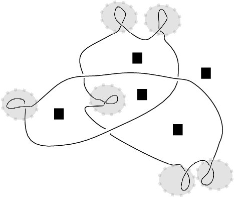
The diagram in Figure 5 is decorated with gray disks and black squares. Each gray disk in the trivial knot diagram contains a monogon (i.e. the shape of Reidemeister move I). Each black square indicates one region of the diagram. By deleting all the crossings in the gray disks with $\Omega^{\downarrow}_{1}$ moves, we may easily see that there is a sequence of Reidemeister moves I and III that transforms the diagram depicted in Figure 5 into the trivial knot diagram without a crossing.

As in Figure 6, we consider $n$-times connected sums of the trivial knot diagram depicted in Figure 5. Note that every region with a black square in the diagram has greater than or equal to $4$ adjacent crossings.

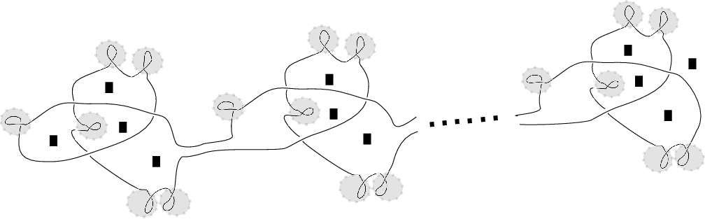
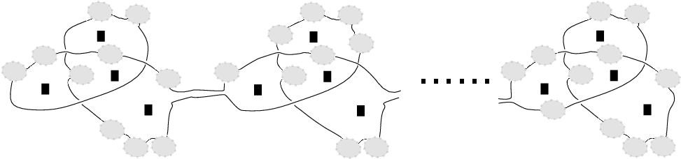
We assume that, the trivial knot diagram depicted in Figure 6 that has neither gray disks nor black squares may be turned into the trivial knot diagram without a crossing by a sequence of $\Omega_{1}^{\uparrow}$ moves, followed by a sequence of $\Omega_{3}$ moves, followed by a sequence of $\Omega_{1}^{\downarrow}$ moves. To clarify the contradiction of the assumption, we are going to add gray disks and black squares to the trivial knot diagram we assumed above as in Figure 6, and replace the ordinary ordered sequence with the ordinary ordered sequence of colored Reidemeister moves, which is the same sequence as the previous ordinary ordered sequence when we ignore gray disks and black squares. We may replace $\Omega_{1}^{\uparrow}$ moves in the ordinary ordered sequence with colored $\Omega_{1}$ moves which are the same moves as the $\Omega_{1}^{\uparrow}$ moves when we ignore gray disks and black squares, since colored $\Omega_{1}^{\uparrow}$ moves defined in Figure 4 have all possibilities of locations of gray disks. (To be clear, when the local disk where we apply an $\Omega_{1}^{\uparrow}$ move in the ordinary ordered sequence is covered by a gray disk, we apply the colored $\Omega_{1}^{\uparrow}$ move located at the lower left in Figure 4 that is the same move as the $\Omega_{1}^{\uparrow}$ move when we ignore gray disks and black squares. When the local disk where we apply an $\Omega_{1}^{\uparrow}$ move in the ordered sequence is not covered by a gray disk, by adjusting the location of the local disk, the local disk may be taken as not being covered by a gray disk. In this case, we apply the colored $\Omega_{1}^{\uparrow}$ move located at the upper left in Figure 4 that is the same move as the $\Omega_{1}^{\uparrow}$ move when we ignore gray disks and black squares.) By applying the sequence of colored $\Omega_{1}^{\uparrow}$ moves as written above, the resulting colored diagram is as in Figure 7, where finitely many gray disks are added and any region with a black square is NOT covered by a gray disk.

$\Omega_{3}$ moves in the ordinary ordered sequence may be replaced with colored $\Omega_{3}$ moves which are the same moves as the $\Omega_{3}$ moves when we ignore gray disks and black squares, since every region with a black square have greater than or equal to $4$ vertices in the process and the $\Omega_{3}$ moves occur only inside the gray disks.

$\Omega_{1}^{\downarrow}$ moves in the ordinary ordered sequence may be replaced with colored $\Omega_{1}^{\downarrow}$ moves which are the same moves as the $\Omega_{1}^{\downarrow}$ moves when we ignore gray disks and black squares, since every region with a black square has greater than or equal to $2$ vertices in the process and the $\Omega_{1}^{\downarrow}$ moves occur only inside the gray disks.

In the whole process written above, every region with a black square does not vanish. This fact contradicts the assumption that the trivial knot diagram depicted in Figure 6 (that has neither gray disks nor black squares) may be turned into the trivial knot diagram without a crossing by a sequence of $\Omega_{1}^{\uparrow}$ moves, followed by a sequence of $\Omega_{3}$ moves, followed by a sequence of $\Omega_{1}^{\downarrow}$ moves. Thus, there is no ordinary ordered sequence that transforms the diagram depicted in Figure 6 into the trivial knot diagram without a crossing.

∎

An $\Omega_{1}^{\uparrow}$ move may be applied at a trivial $1$-tangle diagram without a crossing. This means that there are two trivial $1$-tangle diagrams without a crossing in $D$, where the two $\Omega_{1}^{\uparrow}$ moves are applied. The two $\Omega_{1}^{\uparrow}$ moves may be applied at the same time, since the two local disks may be taken as disjoint. Thus, Lemma 4.3 has been proven.

∎

By using Lemma 4.3 $n$ times, we can prove Lemma 4.4 easily. ∎

When the two local regions of the $\Omega_{1}^{\uparrow}$ move and the $\Omega_{3}$ move in $D$ may be taken as disjoint, we may apply the two local moves separately. This means that the resulting diagram may be taken as $D_{3}$.

When the two local regions of the $\Omega_{1}^{\uparrow}$ move and the $\Omega_{3}$ move in $D_{1}$ may not be taken as disjoint, the local region of the $\Omega_{1}^{\uparrow}$ move in $D_{1}$ may be taken as a rectangle. We may consider the rectangle and the local disk of the $\Omega_{3}$ move in $D_{1}$ as a new $\Omega_{3}^{*}$ move from $D_{1}$ (to $D_{3}$). The difference between the $D_{3}$ appeared right above and $D_{2}$ is just an $\Omega_{1}^{\uparrow}$ move. Thus, Lemma 4.5 has been proven. ∎

By applying Lemma 4.5 and Remark 4.6 $n$$\times$$m$ times, we may prove Lemma 4.7 easily.

∎

By Definition 4.2, the same two link diagrams are an example of two link diagrams that have an I-generalized ordered sequence (i.e. no move) between them.

Let $D_{1}$, $D_{2}$ be two link diagrams that are transformed into each other by applying an I-generalized ordered sequence. Let $\mathcal{D}_{3}$ be the set of link diagrams that are transformed from $D_{2}$ by an $\Omega_{1}^{\uparrow}$ move or an $\Omega_{1}^{\downarrow}$ move or an $\Omega_{3}$ move. From here onward, to prove Theorem 4.9, we are going to check that there exists a new I-generalized ordered sequence that transforms $D_{1}$ into every diagram of $\mathcal{D}_{3}$.

When a diagram $D_{3}$ of $\mathcal{D}_{3}$ is transformed from $D_{2}$ with an $\Omega_{1}^{\downarrow}$ move, the sequence that consists of the I-generalized ordered sequence we assumed right above and the $\Omega_{1}^{\downarrow}$ move is the new I-generalized ordered sequence that transforms $D_{1}$ into $D_{3}$. Moreover, in this argument, since $\Omega_{1}^{\downarrow}$ move is added to both the sequence of finitely many Reidemeister moves I, III and the I-generalized ordered sequence, the numbers of $\Omega_{1}^{\downarrow}$ moves in the two resulting sequences remain the same. In this argument, the numbers of $\Omega_{1}^{\downarrow}$ moves and $\Omega_{3}^{*}$ moves and $\Omega_{3}$ moves do not change.

When a diagram $D_{3}$ of $\mathcal{D}_{3}$ is transformed from $D_{2}$ with an $\Omega_{1}^{\uparrow}$ move, by using Lemma 4.4 and Lemma 4.7 repeatedly on the I-generalized ordered sequence that transforms $D_{1}$ into $D_{2}$ and the $\Omega_{1}^{\uparrow}$ move that transforms $D_{2}$ into $D_{3}$, we may construct a new I-generalized sequence that transforms $D_{1}$ into $D_{3}$. Moreover, in this argument, since an $\Omega_{1}^{\uparrow}$ move is added to both the sequence of finitely many Reidemeister moves I, III and the I-generalized ordered sequence, the numbers of $\Omega_{1}^{\uparrow}$ moves in the two resulting sequences remain the same. In this argument, the numbers of $\Omega_{1}^{\downarrow}$ moves and $\Omega_{3}^{*}$ moves and $\Omega_{3}$ moves do not change.

When a diagram $D_{3}$ of $\mathcal{D}_{3}$ is transformed from $D_{2}$ by an $\Omega_{3}$ move, by using Lemma 4.5 repeatedly, we may construct a new I-generalized ordered sequence that transforms $D_{1}$ into $D_{3}$. Moreover, in this argument, since the $\Omega_{3}$ move is added to the sequence of finitely many Reidemeister moves I, III and an $\Omega_{3}^{*}$ move is added to the I-generalized ordered sequence, the number of $\Omega_{3}$ moves and the number of $\Omega_{3}^{*}$ moves remain the same. In this argument, the numbers of $\Omega_{1}^{\downarrow}$ moves and $\Omega_{3}^{*}$ moves and $\Omega_{3}$ moves do not change.

Thus, The proof of Thoerem 4.9 is completed. ∎

References

- [1] A. Coward, Ordering the Reidemesiter moves of a classical knot. Alg. Geom. Topol. 6 (2006) 659-671.
- [2] A. Coward and M. Lackenby, An upper bound on Reidemeister moves, Amer. J. Math. 136 (2014) 102.
- [3] C. Hayashi and M. Hayashi. Minimal sequeces of Reidemeister moves on diagrams of torus knots. Proc. Amer. Math. Soc. 139:2605-2614, 2011. arXiv:1003.1349.
- [4] J. Carter, M. Elhamdadi, M. Saito, S. Satoh, A lower bound for the number of Reidemeister moves of type III. Topology Appl. 153 (2006) 2788-2794.
- [5] J. Gold, A bound for orderings of Reidemeister moves. Algebr. Geom. Topol. 13 (2013) 3099-3110.
- [6] K. Reidemeister, Knotten und Gruppen, abh. Math. Sem. Univ. Hamburg 5 (1927) 7-23.
- [7] K. Sasaki, On link diagrams that are minimal with respect to Reidemeister moves I and II, preprint. arXiv:1612.00764.