跳到论文正文
W Papers独立论文阅读器 arXiv:2205.06482 论文正文 计算阅读时间 · 0%
引用这篇论文根据当前论文元数据生成,正式投稿前建议核对。


License: arXiv.org perpetual non-exclusive license
arXiv:2205.06482v2 [cs.IT] 12 Jun 2022

Opportunistic Routing Aided Cooperative Communication Network with Energy Harvesting

Wannian An    Chen Dong*    Xiaodong Xu    Chao Xu    Shujun Han    and Lei Teng Thanks: This work was supported in part by $∼$. (Corresponding author: Chen Dong.) Wannian An, Chen Dong, Xiaodong Xu, Shujun Han and Lei Teng are with the State Key Laboratory of Networking and Switching Technology, Beijing University of Posts and Telecommunications, Beijing, 100876, China. (e-mail: anwannian2021@bupt.edu.cn; dongchen@bupt.edu.cn; xuxiaodong@bupt.edu.cn; hanshujun@bupt.edu.cn; tenglei@bupt.edu.cn;). Chao Xu is with the School of Electronics and Computer Science, University of Southampton, SO17 1BJ Southampton, U.K. (e-mail: cx1g08@ecs.soton.ac.uk).
Abstract

In this paper, a cooperative communication network based on energy-harvesting (EH) decode-and-forward (DF) relays that harvest energy from the ambience using buffers with harvest-store-use (HSU) architecture is considered. An opportunistic routing (OR) protocol, which selects the transmission path of packet based on the node transmission priority, is proposed to improve data delivery in this network. Additionally, an algorithm based on state transition matrix (STM) is proposed to obtain the probability distribution of the candidate broadcast node set. Based on the probability distribution, the existence conditions and the theoretical expressions for the limiting distribution of energy in energy buffers using discrete-time continuous-state space Markov chain (DCSMC) model are derived. Furthermore, the closed-form expressions for network outage probability and throughput are obtained with the help of the limiting distributions of energy stored in buffers. Numerous experiments have been performed to validate the derived theoretical expressions.

Index Terms: 
Energy-harvesting, opportunistic routing, state transition matrix, integral equation.

I Introduction

In recent years, as a promising technology, energy-harvesting (EH) has drawn researchers’ substantial attention due to its capability of harvesting energy from the surrounding ambient energy sources such as light energy, thermal energy and radio frequency (RF) energy, etc. [1]. Specifically, EH is widely employed in cooperative wireless communication to prolong the lifetime of traditional energy-constrained cooperative wireless communication networks [2].

The relay selection method considering both the energy state of relay buffer and channel state information (CSI) for EH wireless body area network is shown in [3]. In [4] and [5], the power splitting protocol is employed at the EH relay of the EH-based cooperative communication network to obtain a tradeoff between the transmission energy and decoding energy. In these studies mentioned above, the energy is harvested with the harvest-use (HU) structure, which means that the harvested energy will be used immediately.

Another efficient method of harvesting energy from the environment is to use the harvest-store-use (HSU) architecture, which allows the harvested energy to be stored in an energy buffer or super-capacitor for later use. A wireless powered communication system with an EH node using HSU architecture, which harvests energy from the RF signals in the downlink and uses the stored energy to transmit data in the uplink, is considered in [6], [7] and [8], where the limiting distribution of stored energy in energy buffer at the EH node is derived using discrete-time continuous-state space Markov chain (DCSMC) model. The online and offline optimization algorithms for joint relay selection and power control have been discussed in [9], which aim to maximize the end-to-end system throughput under the constraints of data and energy storage. In [10], an EH-based two-way relaying network is studied, where the relay uses the energy harvested from ambient RF signals to drastically reduce the battery energy consumption. In [11], two time switching policies of the EH relay equipped with energy and data buffers are proposed to maximize the throughput of the cooperative wireless network. To improve the performance of the energy-constrained cooperative communication network, [12] proposes a relay selection scheme based on the status of both energy buffer and data buffer. A cooperative cognitive radio network with two Internet of Things (IoT) devices serving as the relays has been investigated in [13], where the IoT devices employ a time-splitting-based approach for harvesting energy from the RF signals received from a pair of primary users and processing information. Furthermore, the exact expressions of outage probability for the IoT cooperative communication system under Nakagami-m fading is derived.

In these works mentioned above, when the path loss in practical communication link is high, it is not efficient for the relays to harvest energy from RF signals received from the source nodes [14]. Another strategy with greater practical interest is to build the self-sustaining node (SSN) which harvests energy from the ambience. More explicitly, the two-hop relay networks with an HSU-architecture-based EH relay are considered in [15], [16] and [17], where the theoretical expressions for the limiting distribution of energy stored in buffer employing best-effort and on-off policies are derived to analyze the system outage probability and throughput. Different from [16], a feedback strategy is introduced into the system considered in [17], which further improves the spectral efficiency of the system. Furthermore, [18] and [19] introduce the two-hop relay networks with a self-sustaining source and a self-sustaining relay, where both the source and the relay harvest energy from the ambience. In [20] and [21], the performance of a two-hop relay network with a self-sustaining source harvesting energy from the ambience and a data buffer-aided relay is analyzed, where three simple link selection schemes based on buffer status or channel knowledge are adopted to maximize the throughput of the relay network.

It can be found that the above studies are mainly based on a wireless two-hop relay network with relays with the same priority (i.e. they cannot communicate with each other). However, the practical wireless cooperative network often utilizes the wireless multi-hop network with distributed topology, such as the sensor network [22]. For the sake of further improving performance, the wireless multi-hop network based on opportunistic routing (OR) protocol has been widely studied. Specifically, an efficient OR protocol based on both cross-layer information exchange and energy consumption in an ad hoc network has been studied in [23] and [24]. Additionally, the OR protocol considering both global optimization and local optimization is proposed for the dependent duty-cycled wireless sensor network to minimize the end-to-end latency [25]. In order to realize the tradeoff between routing efficiency and computational complexity, multi-objective optimization and Pareto optimality are introduced into the power control-based OR for wireless ad hoc networks [26]. In [27], the OR utilizing the network-based candidate forwarding set optimization scheme is introduced to reduce the transmission delay and avoid duplicate transmission in wireless multi-hop networks. In order to reduce the energy consumption and improve the data delivery ratio in underwater wireless sensor networks, Coutinho and Boukerche [28] design two candidate set selection heuristics to jointly select the most suitable acoustic modem and next-hop forwarder candidate nodes for the current hop. Furthermore, in [29], a reliable reinforcement learning-based OR is proposed in the underwater acoustic sensor network.

According to the above researches, it can be easily found that although EH and OR have been widely studied in cooperative wireless networks, less attention has been devoted to the joint application of EH and OR in cooperative wireless networks. This article aims to study OR-aided cooperative communication networks with EH. Table I shows the comparison between our work and the above references. More specifically, decode-and-forward (DF) relays are powered by harvested energy from the ambience using the infinite-size buffers with HSU architecture. Additionally, the DCSMC model is used to model energy buffers. The main contributions of this work are as follows:

  1. 1.

    In this paper, a cooperative communication network based on EH DF relays is considered. In order to improve the data delivery in this network, an OR protocol for selecting the packet transmission path based on the node transmission priority is proposed.

  2. 2.

    An algorithm for finding the probability distribution of the candidate broadcast node (CBN) set is proposed based on the STM.

  3. 3.

    Based on the DCSMC model and the probability distribution of the CBN set, the existence conditions and the theoretical expressions for the limiting distribution of energy in energy buffers are derived.

  4. 4.

    Based on the limiting distributions of energy stored in buffers, the closed-form expressions are derived for system outage probability and throughput. Additionally, the derived analytical closed-forms and the theoretical analysis given are numerically validated.

TABLE I: Comparison of references. Where N indicates that the technology is not adopted in the studied system, and Y indicates that the technology is adopted in the studied system.
Reference EH buffer architecture SSN OR
[3], [4], [5] HU N N
[6], [7], [8], [9],
[10], [11], [12], [13]
HSU N N
[15], [16], [17],
[18], [19], [20], [21]
HSU Y N
[23], [24], [25],
[26], [27], [28], [29]
No EH N Y
Our work HSU Y Y

The remainder of this paper is organized as follows. In section II, the system model and the proposed OR protocol is described. In section III, the limiting distributions of energy stored in buffers are shown. In section IV, the expressions are derived for system outage probability and throughput. Simulation and theory performance results are presented in Section V. Finally, the conclusion is presented in Section VI.

N​o​t​a​t​i​o​n​s:Notations: A∼𝒞​𝒩​(0,θ)A\sim\mathcal{CN}(0,\theta) indicates the random variable AA follows the complex Gaussian distribution with mean 0 and variance θ\theta. The absolute value of BB is denoted by |B||B|. 𝔼⁡[⋅]\mathbb{E}[\cdot] denotes the expectation operator. C1∩C2C_{1}\cap C_{2} denotes that both the condition C1C_{1} and the condition C2C_{2} are satisfied, while C1∪C2C_{1}\cup C_{2} means that at least one of condition C1C_{1} and condition C2C_{2} is satisfied. W⁡(⋅)W(\cdot) is the Lambert W function. Boldface capital and lower-case letters stand for matrices and vectors, respectively. In addition, C1¯\overline{C_{1}} represents the opposite of condition C1C_{1}. ||⋅||2||\cdot||_{2} denotes the Euclidean norm of vector.

II System Model and OR Protocol

II-A System Model

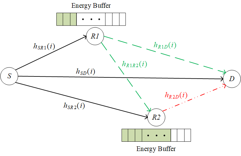
As illustrated in Fig. 1, the network considered in this paper consists of a source node SS, a destination node DD, and two DF relay nodes R​1R1 and R​2R2. In this network, all nodes operate in half duplex mode. The fixed power supply is assumed in both SS and DD, while R​1R1 and R​2R2 are equipped energy buffer shown in Fig. 2 and powered solely by the energy harvested from the ambience. More especially, in each time slot, there is only one activated node transmit signals to corresponding receiving nodes, while the inactive nodes keep silent or receive signals transmitted from the activated node. Additionally, the quasi-static Rayleigh fading channel model is assumed between all nodes, then, the channel coefficients within the ii-th time slot between SS and DD, SS and R​1R1, SS and R​2R2, R​1R1 and R​2R2, R​1R1 and DD, and R​2R2 and DD can be denoted by hS​D​(i)∼𝒞​𝒩​(0,dS​D−α)h_{SD}(i)\sim\mathcal{CN}(0,d_{SD}^{-\alpha}), hS​R​1​(i)∼𝒞​𝒩​(0,dS​R​1−α)h_{SR1}(i)\sim\mathcal{CN}(0,d_{SR1}^{-\alpha}), hS​R​2​(i)∼𝒞​𝒩​(0,dS​R​2−α)h_{SR2}(i)\sim\mathcal{CN}(0,d_{SR2}^{-\alpha}), hR​1​R​2​(i)∼𝒞​𝒩​(0,dR​1​R​2−α)h_{R1R2}(i)\sim\mathcal{CN}(0,d_{R1R2}^{-\alpha}), hR​1​D​(i)∼𝒞​𝒩​(0,dR​1​D−α)h_{R1D}(i)\sim\mathcal{CN}(0,d_{R1D}^{-\alpha}) and hR​2​D​(i)∼𝒞​𝒩​(0,dR​2​D−α)h_{R2D}(i)\sim\mathcal{CN}(0,d_{R2D}^{-\alpha}), respectively, where dn​md_{nm} denotes the distance between the node n∈[S,R​1,R​2]n\in[S,R1,R2] and the node m∈[R​1,R​2,D]m\in[R1,R2,D], and α\alpha is the path-loss parameter.

Refer to caption

Fig. 1: System model.

Refer to caption

Fig. 2: HSU energy harvesting architecture.

The HSU energy harvesting architecture adopted by the energy buffers equipped by R​1R1 and R​2R2 is depicted in Fig. 2. It can be seen from Fig. 2 that the architecture mainly consists of an infinite-size primary energy buffer (PEB) and an infinite-size secondary energy buffer (SEB). Particularly, since the rechargeable energy storage devices are not able to discharge when they are being charged [30], [31], the PEB is utilized to power the node transmitter. In contrast, the harvested energy from the ambient energy source (e.g. the predictable solar energy [32]) needs to be stored in the SEB. In addition, for the sake of achieving the target that energy buffers equipped by R​1R1 and R​2R2 can charge and discharge simultaneously, it is assumed that the PEB may be charged instantaneously by the SEB at the end of one signal time slot. Moreover, the energy loss in the charging process between SEB and PEB and the energy loss in the discharging process between PEB and node transmitter are omitted. In [31], there is evidence to indicate that these assumptions are feasible.

In the proposed cooperative communication network, as shown in Fig. 1, the SS may broadcast unit-energy signals xS​(i)x_{S}(i) to R​1R1, R​2R2 and DD at rate R0R_{0} with the constant transmitting power PSP_{S}. The received signals yS​R​1​(i)y_{SR1}(i), yS​R​2​(i)y_{SR2}(i) and yS​D​(i)y_{SD}(i) at R​1R1, R​2R2 and DD in the ii-th time slot can be represented by

yS​R​1​(i)=PS​hS​R​1​(i)​xS​(i)+nS​R​1​(i),y_{SR1}(i)=\sqrt{P_{S}}h_{SR1}(i)x_{S}(i)+n_{SR1}(i), (1)
yS​R​2​(i)=PS​hS​R​2​(i)​xS​(i)+nS​R​2​(i),y_{SR2}(i)=\sqrt{P_{S}}h_{SR2}(i)x_{S}(i)+n_{SR2}(i), (2)
yS​D​(i)=PS​hS​D​(i)​xS​(i)+nS​D​(i),y_{SD}(i)=\sqrt{P_{S}}h_{SD}(i)x_{S}(i)+n_{SD}(i), (3)

where, nS​R​1​(i)n_{SR1}(i), nS​R​2​(i)n_{SR2}(i) and nS​D​(i)∼𝒞​𝒩​(0,N0)n_{SD}(i)\sim\mathcal{CN}(0,N_{0}) denote the received additive white Gaussian noise (AWGN) at R​1R1, R​2R2 and DD, respectively. Therefore, the instantaneous link signal to noise ratios (SNRs) γS​R​1​(i)\gamma_{SR1}(i), γS​R​2​(i)\gamma_{SR2}(i) and γS​D​(i)\gamma_{SD}(i) at R​1R1, R​2R2 and DD in the ii-th time slot would be given as follows

γS​R​1​(i)=PS​|hS​R​1​(i)|2N0,γS​R​2​(i)=PS​|hS​R​2​(i)|2N0 and γS​D​(i)=PS​|hS​D​(i)|2N0.\begin{split}&\gamma_{SR1}(i)=\frac{P_{S}|h_{SR1}(i)|^{2}}{N_{0}},\quad\gamma_{SR2}(i)=\frac{P_{S}|h_{SR2}(i)|^{2}}{N_{0}}\\ &\mbox{ and }\quad\gamma_{SD}(i)=\frac{P_{S}|h_{SD}(i)|^{2}}{N_{0}}.\end{split} (4)

Because of the DF mode, R​1R1 decodes the received signals xS​(i)x_{S}(i), re-encodes the information into unit-energy symbols xR​1​(i)x_{R1}(i), and then broadcasts xR​1​(i)x_{R1}(i) to R​2R2 and DD at rate R0R_{0} with the constant power PR​1P_{R1}. Additionally, R​2R2 processes the received signals in the same way as R​1R1, and then broadcasts the unit-energy symbols xR​2​(i)x_{R2}(i) to DD at rate R0R_{0} with the constant power PR​2P_{R2}. Next, the received signals yR​1​R​2​(i)y_{R1R2}(i), yR​1​D​(i)y_{R1D}(i) and yR​2​D​(i)y_{R2D}(i) at R​2R2 and DD in the ii-th time slot can be denoted by

yR​1​R​2​(i)=PR​1​hR​1​R​2​(i)​xR​1​(i)+nR​1​R​2​(i),y_{R1R2}(i)=\sqrt{P_{R1}}h_{R1R2}(i)x_{R1}(i)+n_{R1R2}(i), (5)
yR​1​D​(i)=PR​1​hR​1​D​(i)​xR​1​(i)+nR​1​D​(i),y_{R1D}(i)=\sqrt{P_{R1}}h_{R1D}(i)x_{R1}(i)+n_{R1D}(i), (6)
yR​2​D​(i)=PR​2​hR​2​D​(i)​xR​2​(i)+nR​2​D​(i),y_{R2D}(i)=\sqrt{P_{R2}}h_{R2D}(i)x_{R2}(i)+n_{R2D}(i), (7)

where, nR​1​R​2​(i)n_{R1R2}(i), nR​1​D​(i)n_{R1D}(i) and nR​2​D​(i)∼𝒞​𝒩​(0,N0)n_{R2D}(i)\sim\mathcal{CN}(0,N_{0}) denote the received AWGN at R​2R2 and DD, respectively. Similarly, the instantaneous link SNRs γR​1​R​2​(i)\gamma_{R1R2}(i), γR​1​D​(i)\gamma_{R1D}(i) and γR​2​D​(i)\gamma_{R2D}(i) at R​2R2 and DD can be expressed as follows

γR​1​R​2​(i)=PR​1​|hR​1​R​2​(i)|2N0,γR​1​D​(i)=PR​1​|hR​1​D​(i)|2N0 and γR​2​D​(i)=PR​2​|hR​2​D​(i)|2N0.\begin{split}&\gamma_{R1R2}(i)=\frac{P_{R1}|h_{R1R2}(i)|^{2}}{N_{0}},\quad\gamma_{R1D}(i)=\frac{P_{R1}|h_{R1D}(i)|^{2}}{N_{0}}\\ &\mbox{ and }\quad\gamma_{R2D}(i)=\frac{P_{R2}|h_{R2D}(i)|^{2}}{N_{0}}.\end{split} (8)

The time slot diagram of the proposed cooperative communication network is shown in Fig. 3, where one time slot consists of pilot broadcasting sub-slot t​1t1, packet broadcasting sub-slot t​2t2 and positive acknowledgement (ACK) or negative acknowledgement (NACK) broadcasting sub-slot t​3t3. Specifically, in sub-slot t​1t1, nodes DD, R​1R1 and R​2R2 need to broadcast the pilot signals orderly so that each node of this network can know the CSI between itself and other nodes. In sub-slot t​2t2, using the OR protocol described in subsection II B, at most one node is selected to broadcast the packet while the other nodes keep silent. From Fig. 3 it can be seen that SS, R​1R1 and R​2R2 are selected to broadcast the packet in time slot T​1T1, time slot T​2T2 and time slot T​3T3 respectively. In sub-slot t​3t3, nodes DD, R​1R1 and R​2R2 broadcast ACK or NACK signals orderly. In particular, when the instantaneous link SNR at the receiving node is not less than the threshold Γt​h=2R0−1\Gamma_{th}=2^{R_{0}}-1, ACK signals would be broadcasted by the receiving node as the sign of successful packet reception. Otherwise, NACK signals would be broadcasted by the receiving node as the sign of the packet reception failure.

Refer to caption

Fig. 3: System time slot diagram. Where one time slot consists of pilot broadcasting sub-slot t​1t1, packet broadcasting sub-slot t​2t2 and positive acknowledgement (ACK) or negative acknowledgement (NACK) broadcasting sub-slot t​3t3. Especially, in time slot T​1T1, time slot T​2T2 and time slot T​3T3, SS, R​1R1 and R​2R2 are selected to broadcast the packet, respectively.

II-B OR Protocol

TABLE II: The OR Protocol. In the current time slot, the protocol determines the broadcast node (BN) B​N​(i)BN(i) and effective transmission according to the known candidate broadcast node (CBN) set S​(i)\textbf{S}(i) and the known conditions (energy information stored by relay nodes and channel information), and further obtains the CBN set S​(i+1)\textbf{S}(i+1) of the next time slot.
  CBN set S​(i)\textbf{S}(i)   Conditions   BN B​N​(i)BN(i)   Effective transmission   CBN set S​(i+1)\textbf{S}(i+1)
s1={S}\textbf{s}_{1}=\{\mbox{S}\} C1​(i):γS​D​(i)≥Γt​hC_{1}(i):\gamma_{SD}(i)\geq\Gamma_{th} S S→\rightarrowD s1={S}\textbf{s}_{1}=\{\mbox{S}\}
C2​(i):γS​D​(i)<Γt​h∩γS​R​1​(i)≥Γt​h∩γS​R​2​(i)<Γt​hC_{2}(i):\gamma_{SD}(i)<\Gamma_{th}\cap\gamma_{SR1}(i)\geq\Gamma_{th}\cap\gamma_{SR2}(i)<\Gamma_{th} S→\rightarrowR1 s2={S,R1}\textbf{s}_{2}=\{\mbox{S,R1}\}
C3​(i):γS​D​(i)<Γt​h∩γS​R​1​(i)<Γt​h∩γS​R​2​(i)≥Γt​hC_{3}(i):\gamma_{SD}(i)<\Gamma_{th}\cap\gamma_{SR1}(i)<\Gamma_{th}\cap\gamma_{SR2}(i)\geq\Gamma_{th} S→\rightarrowR2 s3={S,R2}\textbf{s}_{3}=\{\mbox{S,R2}\}
C4​(i):γS​D​(i)<Γt​h∩γS​R​1​(i)≥Γt​h∩γS​R​2​(i)≥Γt​hC_{4}(i):\gamma_{SD}(i)<\Gamma_{th}\cap\gamma_{SR1}(i)\geq\Gamma_{th}\cap\gamma_{SR2}(i)\geq\Gamma_{th} S→\rightarrowR1,R2 s4={S,R1,R2}\textbf{s}_{4}=\{\mbox{S,R1,R2}\}
others ≃\simeq ≃\simeq s1={S}\textbf{s}_{1}=\{\mbox{S}\}
s2={S,R1}\textbf{s}_{2}=\{\mbox{S,R1}\} C1​(i):γS​D​(i)≥Γt​hC_{1}(i):\gamma_{SD}(i)\geq\Gamma_{th} S S→\rightarrowD s1={S}\textbf{s}_{1}=\{\mbox{S}\}
C5​(i):γS​D​(i)<Γt​h∩B1​(i)≥M1∩γR​1​D​(i)≥Γt​hC_{5}(i):\gamma_{SD}(i)<\Gamma_{th}\cap B_{1}(i)\geq M_{1}\cap\gamma_{R1D}(i)\geq\Gamma_{th} R1 R1→\rightarrowD
C6​(i):γS​D​(i)<Γt​h∩B1​(i)≥M1∩γR​1​D​(i)<Γt​hC_{6}(i):\gamma_{SD}(i)<\Gamma_{th}\cap B_{1}(i)\geq M_{1}\cap\gamma_{R1D}(i)<\Gamma_{th}
∩γS​R​2​(i)≥Γt​h\cap\gamma_{SR2}(i)\geq\Gamma_{th}
S S→\rightarrowR2 s4={S,R1,R2}\textbf{s}_{4}=\{\mbox{S,R1,R2}\}
C7​(i):γS​D​(i)<Γt​h∩B1​(i)<M1∩γS​R​2​(i)≥Γt​hC_{7}(i):\gamma_{SD}(i)<\Gamma_{th}\cap B_{1}(i)<M_{1}\cap\gamma_{SR2}(i)\geq\Gamma_{th}
C8​(i):γS​D​(i)<Γt​h∩B1​(i)≥M1∩γR​1​D​(i)<Γt​hC_{8}(i):\gamma_{SD}(i)<\Gamma_{th}\cap B_{1}(i)\geq M_{1}\cap\gamma_{R1D}(i)<\Gamma_{th}
∩γS​R​2​(i)<Γt​h∩γR​1​R​2​(i)≥Γt​h\cap\gamma_{SR2}(i)<\Gamma_{th}\cap\gamma_{R1R2}(i)\geq\Gamma_{th}
R1 R1→\rightarrowR2
others ≃\simeq ≃\simeq s2={S,R1}\textbf{s}_{2}=\{\mbox{S,R1}\}
s3={S,R2}\textbf{s}_{3}=\{\mbox{S,R2}\} C1​(i):γS​D​(i)≥Γt​hC_{1}(i):\gamma_{SD}(i)\geq\Gamma_{th} S S→\rightarrowD s1={S}\textbf{s}_{1}=\{\mbox{S}\}
C9​(i):γS​D​(i)<Γt​h∩B2​(i)≥M2∩γR​2​D​(i)≥Γt​hC_{9}(i):\gamma_{SD}(i)<\Gamma_{th}\cap B_{2}(i)\geq M_{2}\cap\gamma_{R2D}(i)\geq\Gamma_{th} R2 R2→\rightarrowD
others ≃\simeq ≃\simeq s3={S,R2}\textbf{s}_{3}=\{\mbox{S,R2}\}
s4={S,R1,R2}\textbf{s}_{4}=\{\mbox{S,R1,R2}\} C1​(i):γS​D​(i)≥Γt​hC_{1}(i):\gamma_{SD}(i)\geq\Gamma_{th} S S→\rightarrowD s1={S}\textbf{s}_{1}=\{\mbox{S}\}
C9​(i):γS​D​(i)<Γt​h∩B2​(i)≥M2∩γR​2​D​(i)≥Γt​hC_{9}(i):\gamma_{SD}(i)<\Gamma_{th}\cap B_{2}(i)\geq M_{2}\cap\gamma_{R2D}(i)\geq\Gamma_{th} R2 R2→\rightarrowD
C10​(i):γS​D​(i)<Γt​h∩B2​(i)≥M2∩γR​2​D​(i)<Γt​hC_{10}(i):\gamma_{SD}(i)<\Gamma_{th}\cap B_{2}(i)\geq M_{2}\cap\gamma_{R2D}(i)<\Gamma_{th}
∩B1​(i)≥M1∩γR​1​D​(i)≥Γt​h\cap B_{1}(i)\geq M_{1}\cap\gamma_{R1D}(i)\geq\Gamma_{th}
R1 R1→\rightarrowD
C11​(i):γS​D​(i)<Γt​h∩B2​(i)<M2∩B1​(i)≥M1C_{11}(i):\gamma_{SD}(i)<\Gamma_{th}\cap B_{2}(i)<M_{2}\cap B_{1}(i)\geq M_{1}
∩γR​1​D​(i)≥Γt​h\cap\gamma_{R1D}(i)\geq\Gamma_{th}
others ≃\simeq ≃\simeq s4={S,R1,R2}\textbf{s}_{4}=\{\mbox{S,R1,R2}\}

In this section, the OR protocol is proposed. In the cooperative communication network shown in Fig. 1, it is first assumed that S always has the packet to be transmitted. Secondly, when transmitting the same packet to the same node, SS has the highest transmission priority, R​2R2 has the second priority, and R​1R1 has the lowest priority. This is because SS has fixed power support and can transmit the packet to R​1R1, R​2R2 and DD. Compared with SS, EH-based R​1R1 can transmit the packet to R​2R2 and DD, while EH-based R​2R2 can only transmit the packet to DD. Third, as long as DD receives the packet, SS would transmit a new packet in the next time slot. In addition, the transmitting node which has the packet to be forwarded is named as CBN, and the node which can receive the packet transmitted by the CBN is named the neighbouring node of the CBN. The main procedures of OR protocol are divided into the following three steps:

  1. 1) :

    Determine the CBN set S​(i)∈{s1,s2,s3,s4}\textbf{S}(i)\in\{\textbf{s}_{1},\textbf{s}_{2},\textbf{s}_{3},\textbf{s}_{4}\} in the current time slot, where s1={S}\textbf{s}_{1}=\{S\}, s2={S,R​1}\textbf{s}_{2}=\{S,R1\}, s3={S,R​2}\textbf{s}_{3}=\{S,R2\}, s4={S,R​1,R​2}\textbf{s}_{4}=\{S,R1,R2\}.

  2. 2) :

    According to the channel informations between nodes, the stored energy B1​(i)B_{1}(i) of R​1R1 and the stored energy B2​(i)B_{2}(i) of R​2R2, in the current time slot, the broadcast node (BN) BN(i)∈{S,R1,R2,≃}BN(i)\in\{S,R1,R2,\simeq\} is selected from the CBN set S​(i)\textbf{S}(i), where ≃\simeq indicates that there is no node is selected to broadcast the packet in the current time slot.

  3. 3) :

    Determine the effective transmission and get CBN set S​(i+1)∈{s1,s2,s3,s4}\textbf{S}(i+1)\in\{\textbf{s}_{1},\textbf{s}_{2},\textbf{s}_{3},\textbf{s}_{4}\} in the next time slot.

More especially, Table II describes the OR protocol in detail, where M1M_{1} and M2M_{2} denote the energy consumed by R​1R1 and R​2R2 to broadcast the packet in one time slot, respectively. Moreover, M1M_{1} and M2M_{2} are numerically equal to PR​1P_{R1} and PR​2P_{R2}, respectively.

III Limiting Distribution of Energy

This section is concerned with the limiting distributions of stored energy in the infinite-size energy buffers with HSU architecture. Specially, it is assumed that X1​(i)X_{1}(i) and X2​(i)X_{2}(i) are the energy harvested by R​1R1 and R​2R2 from the surrounding environment in one time slot, respectively. Moreover, X1​(i)X_{1}(i) and X2​(i)X_{2}(i) are exponentially distributed random variables (as in both [30] and [31]) with means 𝔼⁡[X1​(i)]=1/λ1\mathbb{E}[X_{1}(i)]=1/\lambda_{1} and 𝔼⁡[X2​(i)]=1/λ2\mathbb{E}[X_{2}(i)]=1/\lambda_{2}, respectively. So that the probability density function (PDF) of X1​(i)X_{1}(i) and X2​(i)X_{2}(i) can be expressed as follows

fXj(x)=λje−λj​x,x>0,j∈1,2.f_{X_{j}}(x)=\lambda_{j}e^{-\lambda_{j}x},\quad x>0,j\in{1,2}. (9)

III-A Limiting Distribution of R​2R2 Energy

Using the DCSMC on the continuous state space [0,∞)[0,\infty), the dynamic process B2​(i)B_{2}(i) of the energy storage in the infinite-size energy buffer of R​2R2 can be given as follows

B2​(i+1)=B2​(i)+X2​(i),ℙ21B2​(i+1)=B2​(i)−M2+X2​(i),ℙ22\begin{split}&B_{2}(i+1)=B_{2}(i)+X_{2}(i),\quad\mathbb{P}_{21}\\ &B_{2}(i+1)=B_{2}(i)-M_{2}+X_{2}(i),\quad\mathbb{P}_{22}\end{split} (10)

where ℙ21\mathbb{P}_{21} and ℙ22\mathbb{P}_{22} are the conditions required for the storage equations in Eq. (10) to hold according to the OR protocol shown in Table II. And ℙ21\mathbb{P}_{21} and ℙ22\mathbb{P}_{22} can be expressed as follows

ℙ21:⟨(S(i)=s3)∪(S(i)=s4)⟩∩[C1(i)∪⟨C1¯(i)∩(B2(i)≥M2)∩(γR​2​D(i)<Γt​h)⟩∪⟨C1¯(i)∩(B2(i)<M2)⟩]∪(S(i)=s1)∪(S(i)=s2),\begin{split}\mathbb{P}_{21}:\,&\Big\langle\big(\textbf{S}(i)=\textbf{s}_{3}\big)\cup\big(\textbf{S}(i)=\textbf{s}_{4}\big)\Big\rangle\cap\bigg[C_{1}(i)\cup\Big\langle\overline{C_{1}}(i)\\ &\cap\big(B_{2}(i)\geq M_{2}\big)\cap\big(\gamma_{R2D}(i)<\Gamma_{th}\big)\Big\rangle\cup\Big\langle\overline{C_{1}}(i)\\ &\cap\big(B_{2}(i)<M_{2}\big)\Big\rangle\bigg]\cup\big(\textbf{S}(i)=\textbf{s}_{1}\big)\cup\big(\textbf{S}(i)=\textbf{s}_{2}\big),\\ \end{split} (11)
ℙ22:⟨(S​(i)=s3)∪(S​(i)=s4)⟩∩C9​(i).\begin{split}\mathbb{P}_{22}:\,\Big\langle\big(\textbf{S}(i)=\textbf{s}_{3}\big)\cup\big(\textbf{S}(i)=\textbf{s}_{4}\big)\Big\rangle\cap C_{9}(i).\end{split} (12)

where C1​(i)C_{1}(i) and C9​(i)C_{9}(i) are given in Table II.

Let p1p_{1}, p2p_{2}, p3p_{3} and p4p_{4} denote the probabilities Pr{S(i)=s1}\mathrm{Pr}\{\textbf{S}(i)=\textbf{s}_{1}\}, Pr{S(i)=s2}\mathrm{Pr}\{\textbf{S}(i)=\textbf{s}_{2}\}, Pr{S(i)=s3}\mathrm{Pr}\{\textbf{S}(i)=\textbf{s}_{3}\} and Pr{S(i)=s4}\mathrm{Pr}\{\textbf{S}(i)=\textbf{s}_{4}\} in the case of stable energy buffers, respectively, and the values of these probabilities can be obtained in Alg. 1 which is introduced in subsection III C. Then, define ΩS​D=dS​Dα​N0PS\Omega_{SD}=\frac{d_{SD}^{\alpha}N_{0}}{P_{S}}, ΩS​R​2=dS​R​2α​N0PS\Omega_{SR2}=\frac{d_{SR2}^{\alpha}N_{0}}{P_{S}}, ΩS​R​1=dS​R​1α​N0PS\Omega_{SR1}=\frac{d_{SR1}^{\alpha}N_{0}}{P_{S}}, ΩR​1​D=dR​1​Dα​N0M1\Omega_{R1D}=\frac{d_{R1D}^{\alpha}N_{0}}{M_{1}}, ΩR​1​R​2=dR​1​R​2α​N0M1\Omega_{R1R2}=\frac{d_{R1R2}^{\alpha}N_{0}}{M_{1}} and ΩR​2​D=dR​2​Dα​N0M2\Omega_{R2D}=\frac{d_{R2D}^{\alpha}N_{0}}{M_{2}}. Furthermore, let ψ2\psi_{2} denote the energy buffer stabilization parameter for the energy storage process B2​(i)B_{2}(i) in Eq. (10), which can be expressed as follows

ψ2=λ2​M2​[(p3+p4)​(1−e−ΩS​D​Γt​h)​e−ΩR​2​D​Γt​h]=M2​[(p3+p4)​(1−e−ΩS​D​Γt​h)​e−ΩR​2​D​Γt​h]𝔼​[X2​(i)].\begin{split}\psi_{2}&=\lambda_{2}M_{2}\left[\left(p_{3}+p_{4}\right)\left(1-e^{-\Omega_{SD}\Gamma_{th}}\right)e^{-\Omega_{R2D}\Gamma_{th}}\right]\\ &=\frac{M_{2}\left[\left(p_{3}+p_{4}\right)\left(1-e^{-\Omega_{SD}\Gamma_{th}}\right)e^{-\Omega_{R2D}\Gamma_{th}}\right]}{\mathbb{E}[X_{2}(i)]}.\end{split} (13)
Theorem 1

If ψ2≤1\psi_{2}\leq 1, the energy storage process B2​(i)B_{2}(i) in Eq. (10) will not have a stationary distribution. Moreover, after a finite number of time slots, B2​(i)>M2B_{2}(i)>M_{2} almost always hold.

Proof 1

The proof is presented in Appendix A.

Theorem 2

For the storage process B2​(i)B_{2}(i) in Eq. (10), the limiting energy distribution exists with ψ2>1\psi_{2}>1. Furthermore, the limiting PDF of the energy buffer state at R​2R2 can be given by

g2​(x)={1M2​(1−eQ2​x),0≤x<M21M2​−Q2​eQ2​x(b2​λ2+Q2),x≥M2g_{2}(x)=\begin{cases}\dfrac{1}{M_{2}}\left(1-e^{Q_{2}x}\right),&0\leq x<M_{2}\\ \dfrac{1}{M_{2}}\dfrac{-Q_{2}e^{Q_{2}x}}{\left(b_{2}\lambda_{2}+Q_{2}\right)},&x\geq M_{2}\end{cases} (14)

where,

b2=[(p3+p4)​(1−e−ΩS​D​Γt​h)​e−ΩR​2​D​Γt​h],\begin{split}b_{2}=\left[\left(p_{3}+p_{4}\right)\left(1-e^{-\Omega_{SD}\Gamma_{th}}\right)e^{-\Omega_{R2D}\Gamma_{th}}\right],\end{split} (15)

and Q2=−W⁡(−b2​λ2​M2​e−b2​λ2​M2)M2−b2​λ2<0Q_{2}=\frac{-W\left(-b_{2}\lambda_{2}M_{2}e^{-b_{2}\lambda_{2}M_{2}}\right)}{M_{2}}-b_{2}\lambda_{2}<0, satisfying b2​λ2​eQ2​M2=b2​λ2+Q2b_{2}\lambda_{2}e^{Q_{2}M_{2}}=b_{2}\lambda_{2}+Q_{2}. Furthermore, the probabilities Pr{B2(i)≥MR}\mathrm{Pr}\{B_{2}(i)\geq M_{R}\} and Pr{B2(i)<MR}\mathrm{Pr}\{B_{2}(i)<M_{R}\} may be written as follows

Pr{B2(i)≥M2}=∫x=M2∞−Q2​eQ2​xM2​(b2​λ2+Q2)​𝑑x=eQ2​M2M2​(b2​λ2+Q2)=1M2​b2​λ2,\begin{split}\mathrm{Pr}\{B_{2}(i)\geq M_{2}\}&=\int_{x=M_{2}}^{\infty}\dfrac{-Q_{2}e^{Q_{2}x}}{M_{2}\left(b_{2}\lambda_{2}+Q_{2}\right)}\,dx\\ &=\dfrac{e^{Q_{2}M_{2}}}{M_{2}\left(b_{2}\lambda_{2}+Q_{2}\right)}=\dfrac{1}{M_{2}b_{2}\lambda_{2}},\end{split} (16)
Pr{B2(i)<M2}=1−1M2​b2​λ2.\begin{split}\mathrm{Pr}\{B_{2}(i)<M_{2}\}=1-\dfrac{1}{M_{2}b_{2}\lambda_{2}}.\end{split} (17)
Proof 2

The proof is presented in Appendix B.

III-B Limiting Distribution of R​1R1 Energy

Similarly, Let B1​(i)B_{1}(i) denotes the dynamic process of the energy storage in the infinite-size energy buffer of relay R​1R1 using the DCSMC on a continuous state space [0,∞)[0,\infty), which can be given by the storage equation as follows

B1​(i+1)=B1​(i)+X1​(i),ℙ11B1​(i+1)=B1​(i)−M1+X1​(i),ℙ12\begin{split}&B_{1}(i+1)=B_{1}(i)+X_{1}(i),\quad\mathbb{P}_{11}\\ &B_{1}(i+1)=B_{1}(i)-M_{1}+X_{1}(i),\quad\mathbb{P}_{12}\end{split} (18)

Where ℙ11\mathbb{P}_{11} and ℙ12\mathbb{P}_{12} are the conditions required for above OR protocol based storage equations to hold, and they are shown in Eq. (19) and Eq. (20), respectively.

ℙ11:(S(i)=s1)∪(S(i)=s3)∪(S(i)=s2)∩{C1(i)∪⟨C1¯(i)∩(B1(i)≥M1)∩(γR​1​D(i)<Γt​h)⟩∩[⟨(γS​R​2(i)<Γt​h)∩(γR​1​R​2(i)<Γt​h)⟩∪(γS​R​2(i)≥Γt​h)]∪⟨C1¯(i)∩(B1(i)<M1)⟩}∪(S(i)=s4)∩{C1(i)∪C9(i)∪C1¯(i)∩[⟨(B2(i)≥M2)∩(γR​2​D(i)<Γt​h)⟩∪(B2(i)<M2)]∩[⟨(B1(i)≥M1)∩(γR​1​D(i)<Γt​h)⟩∪(B1(i)<M1)]}\begin{split}\mathbb{P}_{11}:\,&\big(\textbf{S}(i)=\textbf{s}_{1}\big)\cup\big(\textbf{S}(i)=\textbf{s}_{3}\big)\cup\big(\textbf{S}(i)=\textbf{s}_{2}\big)\cap\Bigg\{C_{1}(i)\cup\Big\langle\overline{C_{1}}(i)\cap\big(B_{1}(i)\geq M_{1}\big)\cap\big(\gamma_{R1D}(i)<\Gamma_{th}\big)\Big\rangle\\ &\cap\bigg[\Big\langle\big(\gamma_{SR2}(i)<\Gamma_{th}\big)\cap\big(\gamma_{R1R2}(i)<\Gamma_{th}\big)\Big\rangle\cup\big(\gamma_{SR2}(i)\geq\Gamma_{th}\big)\bigg]\cup\Big\langle\overline{C_{1}}(i)\cap\big(B_{1}(i)<M_{1}\big)\Big\rangle\Bigg\}\\ &\cup\big(\textbf{S}(i)=\textbf{s}_{4}\big)\cap\Bigg\{C_{1}(i)\cup C_{9}(i)\cup\overline{C_{1}}(i)\cap\bigg[\Big\langle\big(B_{2}(i)\geq M_{2}\big)\cap\big(\gamma_{R2D}(i)<\Gamma_{th}\big)\Big\rangle\cup\big(B_{2}(i)<M_{2}\big)\bigg]\\ &\cap\bigg[\Big\langle\big(B_{1}(i)\geq M_{1}\big)\cap\big(\gamma_{R1D}(i)<\Gamma_{th}\big)\Big\rangle\cup\big(B_{1}(i)<M_{1}\big)\bigg]\Bigg\}\end{split} (19)
ℙ12:[(S​(i)=s2)∩⟨C5​(i)∪C8​(i)⟩]∪[(S​(i)=s4)∩⟨C10​(i)∪C11​(i)⟩].\begin{split}\mathbb{P}_{12}:\,&\bigg[\big(\textbf{S}(i)=\textbf{s}_{2}\big)\cap\Big\langle C_{5}(i)\cup C_{8}(i)\Big\rangle\bigg]\\ &\cup\bigg[\big(\textbf{S}(i)=\textbf{s}_{4}\big)\cap\Big\langle C_{10}(i)\cup C_{11}(i)\Big\rangle\bigg].\end{split} (20)

where C1​(i)C_{1}(i), C5​(i)C_{5}(i), C8​(i)C_{8}(i), C9​(i)C_{9}(i), C10​(i)C_{10}(i) and C11​(i)C_{11}(i) are given in Table II.

The energy buffer stabilization parameter ψ2\psi_{2} for the energy storage process B2​(i)B_{2}(i) of Eq. (18) can be expressed as follows

ψ1=λ1M1(1−e−ΩS​D​Γt​h)[p2e−ΩR​1​D​Γt​h+p2​(1−e−ΩR​1​D​Γt​h)​(1−e−ΩS​R​2​Γt​h)​e−ΩR​1​R​2​Γt​h+p4e−ΩR​1​D​Γt​h(1−e−ΩR​2​D​Γt​hM2​b2​λ2)].\begin{split}\psi_{1}&=\lambda_{1}M_{1}\left(1-e^{-\Omega_{SD}\Gamma_{th}}\right)\bigg[p_{2}e^{-\Omega_{R1D}\Gamma_{th}}\\ &+p_{2}\left(1-e^{-\Omega_{R1D}\Gamma_{th}}\right)\left(1-e^{-\Omega_{SR2}\Gamma_{th}}\right)e^{-\Omega_{R1R2}\Gamma_{th}}\\ &+p_{4}e^{-\Omega_{R1D}\Gamma_{th}}\left(1-\frac{e^{-\Omega_{R2D}\Gamma_{th}}}{M_{2}b_{2}\lambda_{2}}\right)\bigg].\end{split} (21)
Theorem 3

Similarly, for the energy storage process B1​(i)B_{1}(i) in Eq. (18), the stationary distribution does not exist when ψ1≤1\psi_{1}\leq 1, and there is always M1M_{1} amount of energy available in the buffer.

Proof 3

The proof of theorem 3 only needs to replace ℙ21\mathbb{P}_{21} and ℙ22\mathbb{P}_{22} in Eq. (53) with ℙ11\mathbb{P}_{11} and ℙ12\mathbb{P}_{12}, respectively, and the rest is the same as the proof process of theorem 1.

Theorem 4

When, ψ1>1\psi_{1}>1, the limiting distribution of B1​(i)B_{1}(i) exists and the limiting PDF g1​(x)g_{1}(x) of B1​(i)B_{1}(i) can be given by

g1​(x)={1M1​(1−eQ1​x),0≤x<M11M1​−Q1​eQ1​x(b1​λ1+Q1),x≥M1.g_{1}(x)=\begin{cases}\dfrac{1}{M_{1}}\left(1-e^{Q_{1}x}\right),&0\leq x<M_{1}\\ \dfrac{1}{M_{1}}\dfrac{-Q_{1}e^{Q_{1}x}}{\left(b_{1}\lambda_{1}+Q_{1}\right)},&x\geq M_{1}.\end{cases} (22)

where, b1b_{1} is given as follows

b1=(1−e−ΩS​D​Γt​h)[p2e−ΩR​1​D​Γt​h+p2​(1−e−ΩR​1​D​Γt​h)​(1−e−ΩS​R​2​Γt​h)​e−ΩR​1​R​2​Γt​h+p4e−ΩR​1​D​Γt​h(1−e−ΩR​2​D​Γt​hM2​b2​λ2)],\begin{split}b_{1}&=\left(1-e^{-\Omega_{SD}\Gamma_{th}}\right)\bigg[p_{2}e^{-\Omega_{R1D}\Gamma_{th}}\\ &+p_{2}\left(1-e^{-\Omega_{R1D}\Gamma_{th}}\right)\left(1-e^{-\Omega_{SR2}\Gamma_{th}}\right)e^{-\Omega_{R1R2}\Gamma_{th}}\\ &+p_{4}e^{-\Omega_{R1D}\Gamma_{th}}\left(1-\frac{e^{-\Omega_{R2D}\Gamma_{th}}}{M_{2}b_{2}\lambda_{2}}\right)\bigg],\end{split} (23)

and Q1=−W⁡(−b1​λ1​M1​e−b1​λ1​M1)M1−b1​λ1<0Q_{1}=\frac{-W\left(-b_{1}\lambda_{1}M_{1}e^{-b_{1}\lambda_{1}M_{1}}\right)}{M_{1}}-b_{1}\lambda_{1}<0, satisfying b1​λ1​eQ1​M1=b1​λ1+Q1b_{1}\lambda_{1}e^{Q_{1}M_{1}}=b_{1}\lambda_{1}+Q_{1}. In addition, the probabilities Pr{B1(i)≥M1}\mathrm{Pr}\{B_{1}(i)\geq M_{1}\} and Pr{B1(i)<M1}\mathrm{Pr}\{B_{1}(i)<M_{1}\} may be written as follows

Pr{B1(i)≥M1}=∫x=M1∞−Q1​eQ1​xM1​(b1​λ1+Q1)​𝑑x=eQ1​M1M1​(b1​λ1+Q1)=1M1​b1​λ1,\begin{split}\mathrm{Pr}\{B_{1}(i)\geq M_{1}\}&=\int_{x=M_{1}}^{\infty}\dfrac{-Q_{1}e^{Q_{1}x}}{M_{1}\left(b_{1}\lambda_{1}+Q_{1}\right)}\,dx\\ &=\dfrac{e^{Q_{1}M_{1}}}{M_{1}\left(b_{1}\lambda_{1}+Q_{1}\right)}=\dfrac{1}{M_{1}b_{1}\lambda_{1}},\end{split} (24)
Pr{B1(i)<M1}=1−1M1​b1​λ1.\begin{split}\mathrm{Pr}\{B_{1}(i)<M_{1}\}=1-\dfrac{1}{M_{1}b_{1}\lambda_{1}}.\end{split} (25)
Proof 4

The proof is presented in Appendix C.

III-C The Probability Distribution of CBN Set S in the Case of Stable Energy Buffer

The previous theorem 2 and theorem 4 illustrate that after some time slots, the energy buffers in R​1R1 and R​2R2 will reach their own stable states under the condition of ψ1>1\psi_{1}>1 and ψ2>1\psi_{2}>1. Moreover, when the energy buffers in R​1R1 and R​2R2 reach their own stable states, the probability distribution p=[p1,p2,p3,p4]\textbf{p}=[p_{1},p_{2},p_{3},p_{4}] of CBN Set S may be obtained by STM, which is expressed as follows

p​(i+1)=p​(i)​T​(i),\textbf{p}(i+1)=\textbf{p}(i)\textbf{T}(i), (26)

where p​(i)=[p1​(i),p2​(i),p3​(i),p4​(i)]\textbf{p}(i)=[p_{1}(i),p_{2}(i),p_{3}(i),p_{4}(i)] denotes the values of p in the ii-th time slot, p​(i+1)=[p1​(i+1),p2​(i+1),p3​(i+1),p4​(i+1)]\textbf{p}(i+1)=[p_{1}(i+1),p_{2}(i+1),p_{3}(i+1),p_{4}(i+1)] denotes the values of p in the (i+1)(i+1)-th time slot, and T​(i)\textbf{T}(i) is the STM of these probabilities from p​(i)\textbf{p}(i) to p​(i+1)\textbf{p}(i+1). Furthermore, according to table II, the STM T​(i)\textbf{T}(i) can be constructed as follows

T​(i)=[ps1​s1​(i)ps1​s2​(i)ps1​s3​(i)ps1​s4​(i)ps2​s1​(i)ps2​s2​(i)ps2​s3​(i)ps2​s4​(i)ps3​s1​(i)ps3​s2​(i)ps3​s3​(i)ps3​s4​(i)ps4​s1​(i)ps4​s2​(i)ps4​s3​(i)ps4​s4​(i)],\textbf{T}(i)=\begin{bmatrix}p_{\textbf{s}_{1}\textbf{s}_{1}}(i)&p_{\textbf{s}_{1}\textbf{s}_{2}}(i)&p_{\textbf{s}_{1}\textbf{s}_{3}}(i)&p_{\textbf{s}_{1}\textbf{s}_{4}}(i)\\ p_{\textbf{s}_{2}\textbf{s}_{1}}(i)&p_{\textbf{s}_{2}\textbf{s}_{2}}(i)&p_{\textbf{s}_{2}\textbf{s}_{3}}(i)&p_{\textbf{s}_{2}\textbf{s}_{4}}(i)\\ p_{\textbf{s}_{3}\textbf{s}_{1}}(i)&p_{\textbf{s}_{3}\textbf{s}_{2}}(i)&p_{\textbf{s}_{3}\textbf{s}_{3}}(i)&p_{\textbf{s}_{3}\textbf{s}_{4}}(i)\\ p_{\textbf{s}_{4}\textbf{s}_{1}}(i)&p_{\textbf{s}_{4}\textbf{s}_{2}}(i)&p_{\textbf{s}_{4}\textbf{s}_{3}}(i)&p_{\textbf{s}_{4}\textbf{s}_{4}}(i)\end{bmatrix}, (27)

where, the element pI​J​(k)​(I,J∈{s1,s2,s3,s4})p_{IJ}(k)(I,J\in\{\textbf{s}_{1},\textbf{s}_{2},\textbf{s}_{3},\textbf{s}_{4}\}) denotes the probability that the CBN set S​(i)\textbf{S}(i) changes from II in the ii-th time slot to JJ in the (i+1)(i+1)-th time slot, satisfying ∑J∈{s1,s2,s3,s4}pI​J​(i)=1\begin{matrix}\sum_{J\in\{\textbf{s}_{1},\textbf{s}_{2},\textbf{s}_{3},\textbf{s}_{4}\}}p_{IJ}(i)\end{matrix}=1. Furthermore, according to the variables γS​D\gamma_{SD}, γS​R​1\gamma_{SR1}, γS​R​2\gamma_{SR2}, γR​1​D\gamma_{R1D}, γR​1​R​2\gamma_{R1R2}, γR​2​D\gamma_{R2D}, Pr{B2(i)≥M2}\mathrm{Pr}\{B_{2}(i)\geq M_{2}\}, Pr{B1(i)≥M1}\mathrm{Pr}\{B_{1}(i)\geq M_{1}\}, and the OR protocol shown in Table II, pI​J​(i)p_{IJ}(i) may be obtained as follows

ps1​s1​(i)=Pr⁡{γS​D​(i)<Γt​h,γS​R​1​(i)<Γt​h,γS​R​2​(i)<Γt​h}+Pr​{C1​(i)}=(1−e−ΩS​D​Γt​h)​(1−e−ΩS​R​1​Γt​h)​(1−e−ΩS​R​2​Γt​h)+e−ΩS​D​Γt​h,\begin{split}p_{\textbf{s}_{1}\textbf{s}_{1}}(i)&=\mathrm{Pr}\{\gamma_{SD}(i)<\Gamma_{th},\gamma_{SR1}(i)<\Gamma_{th},\gamma_{SR2}(i)<\Gamma_{th}\}\\ &\quad+\mathrm{Pr}\{C_{1}(i)\}\\ &=\left(1-e^{-\Omega_{SD}\Gamma_{th}}\right)\left(1-e^{-\Omega_{SR1}\Gamma_{th}}\right)\left(1-e^{-\Omega_{SR2}\Gamma_{th}}\right)\\ &\quad+e^{-\Omega_{SD}\Gamma_{th}},\end{split} (28)
ps1​s2​(i)=Pr​{C2​(i)}=(1−e−ΩS​D​Γt​h)​e−ΩS​R​1​Γt​h​(1−e−ΩS​R​2​Γt​h),\begin{split}p_{\textbf{s}_{1}\textbf{s}_{2}}(i)&=\mathrm{Pr}\{C_{2}(i)\}\\ &=\left(1-e^{-\Omega_{SD}\Gamma_{th}}\right)e^{-\Omega_{SR1}\Gamma_{th}}\left(1-e^{-\Omega_{SR2}\Gamma_{th}}\right),\end{split} (29)
ps1​s3​(i)=Pr​{C3​(i)}=(1−e−ΩS​D​Γt​h)​(1−e−ΩS​R​1​Γt​h)​e−ΩS​R​2​Γt​h,\begin{split}p_{\textbf{s}_{1}\textbf{s}_{3}}(i)&=\mathrm{Pr}\{C_{3}(i)\}\\ &=\left(1-e^{-\Omega_{SD}\Gamma_{th}}\right)\left(1-e^{-\Omega_{SR1}\Gamma_{th}}\right)e^{-\Omega_{SR2}\Gamma_{th}},\end{split} (30)
ps1​s4​(i)=Pr​{C4​(i)}=(1−e−ΩS​D​Γt​h)​e−ΩS​R​1​Γt​h​e−ΩS​R​2​Γt​h,\begin{split}p_{\textbf{s}_{1}\textbf{s}_{4}}(i)&=\mathrm{Pr}\{C_{4}(i)\}\\ &=\left(1-e^{-\Omega_{SD}\Gamma_{th}}\right)e^{-\Omega_{SR1}\Gamma_{th}}e^{-\Omega_{SR2}\Gamma_{th}},\end{split} (31)

and,

ps2​s1​(i)=Pr⁡{C1​(i)}+Pr⁡{C5​(i)}=e−ΩS​D​Γt​h+(1−e−ΩS​D​Γt​h)​e−ΩR​1​D​Γt​hb1​(i)​λ1​M1,\begin{split}p_{\textbf{s}_{2}\textbf{s}_{1}}(i)&=\mathrm{Pr}\{C_{1}(i)\}+\mathrm{Pr}\{C_{5}(i)\}\\ &=e^{-\Omega_{SD}\Gamma_{th}}+\frac{\left(1-e^{-\Omega_{SD}\Gamma_{th}}\right)e^{-\Omega_{R1D}\Gamma_{th}}}{b_{1}(i)\lambda_{1}M_{1}},\end{split} (32)
ps2​s2​(i)=Pr{C1¯(i),B1(i)≥M1,γR​1​D(i)<Γt​h,γS​R​2(i)<Γt​h,γR​1​R​2(i)<Γt​h}+Pr⁡{C1¯​(i),B1​(i)<M1,γS​R​2​(i)<Γt​h}=(1−e−ΩS​D​Γt​h)​(1−e−ΩS​R​2​Γt​h)×[(1−e−ΩR​1​D​Γt​h)​(1−e−ΩR​1​R​2​Γt​h)b1​(i)​λ1​M1+(1−1b1​(i)​λ1​M1)],\begin{split}p_{\textbf{s}_{2}\textbf{s}_{2}}(i)&=\mathrm{Pr}\{\overline{C_{1}}(i),B_{1}(i)\geq M_{1},\gamma_{R1D}(i)<\Gamma_{th},\\ &\quad\gamma_{SR2}(i)<\Gamma_{th},\gamma_{R1R2}(i)<\Gamma_{th}\}\\ &\quad+\mathrm{Pr}\{\overline{C_{1}}(i),B_{1}(i)<M_{1},\gamma_{SR2}(i)<\Gamma_{th}\}\\ &=\left(1-e^{-\Omega_{SD}\Gamma_{th}}\right)\left(1-e^{-\Omega_{SR2}\Gamma_{th}}\right)\\ &\quad\times\bigg[\frac{\left(1-e^{-\Omega_{R1D}\Gamma_{th}}\right)\left(1-e^{-\Omega_{R1R2}\Gamma_{th}}\right)}{b_{1}(i)\lambda_{1}M_{1}}\\ &\quad+\left(1-\frac{1}{b_{1}(i)\lambda_{1}M_{1}}\right)\bigg],\end{split} (33)
ps2​s4​(i)=Pr⁡{C6​(i)}+Pr⁡{C7​(i)}+Pr⁡{C8​(i)}=(1−e−ΩS​D​Γt​h)[e−ΩS​R​2​Γt​h(1−e−ΩR​1​D​Γt​hb1​(i)​λ1​M1)+(1−e−ΩR​1​D​Γt​h)​(1−e−ΩS​R​2​Γt​h)​e−ΩR​1​R​2​Γt​hb1​(i)​λ1​M1],\begin{split}p_{\textbf{s}_{2}\textbf{s}_{4}}(i)&=\mathrm{Pr}\{C_{6}(i)\}+\mathrm{Pr}\{C_{7}(i)\}+\mathrm{Pr}\{C_{8}(i)\}\\ &=\left(1-e^{-\Omega_{SD}\Gamma_{th}}\right)\bigg[e^{-\Omega_{SR2}\Gamma_{th}}\left(1-\frac{e^{-\Omega_{R1D}\Gamma_{th}}}{b_{1}(i)\lambda_{1}M_{1}}\right)\\ &+\frac{\left(1-e^{-\Omega_{R1D}\Gamma_{th}}\right)\left(1-e^{-\Omega_{SR2}\Gamma_{th}}\right)e^{-\Omega_{R1R2}\Gamma_{th}}}{b_{1}(i)\lambda_{1}M_{1}}\bigg],\end{split} (34)
ps2​s3​(i)=0,\begin{split}p_{\textbf{s}_{2}\textbf{s}_{3}}(i)&=0,\end{split} (35)

and,

ps3​s1​(i)=Pr⁡{C1​(i)}+Pr⁡{C9​(i)}=e−ΩS​D​Γt​h+(1−e−ΩS​D​Γt​h)​e−ΩR​2​D​Γt​hb2​(i)​λ2​M2,\begin{split}p_{\textbf{s}_{3}\textbf{s}_{1}}(i)&=\mathrm{Pr}\{C_{1}(i)\}+\mathrm{Pr}\{C_{9}(i)\}\\ &=e^{-\Omega_{SD}\Gamma_{th}}+\frac{\left(1-e^{-\Omega_{SD}\Gamma_{th}}\right)e^{-\Omega_{R2D}\Gamma_{th}}}{b_{2}(i)\lambda_{2}M_{2}},\end{split} (36)
ps3​s3​(i)=Pr⁡{C1¯​(i),B2​(i)<M2}+Pr⁡{C1¯​(i),B2​(i)≥M2,γR​2​D​(i)<Γt​h}=(1−e−ΩS​D​Γt​h)​(1−e−ΩR​2​D​Γt​hb2​(i)​λ2​M2),\begin{split}p_{\textbf{s}_{3}\textbf{s}_{3}}(i)&=\mathrm{Pr}\{\overline{C_{1}}(i),B_{2}(i)<M_{2}\}\\ &\quad+\mathrm{Pr}\{\overline{C_{1}}(i),B_{2}(i)\geq M_{2},\gamma_{R2D}(i)<\Gamma_{th}\}\\ &=\left(1-e^{-\Omega_{SD}\Gamma_{th}}\right)\left(1-\frac{e^{-\Omega_{R2D}\Gamma_{th}}}{b_{2}(i)\lambda_{2}M_{2}}\right),\end{split} (37)
ps3​s2​(i)=ps3​s4​(i)=0,\begin{split}p_{\textbf{s}_{3}\textbf{s}_{2}}(i)=p_{\textbf{s}_{3}\textbf{s}_{4}}(i)=0,\end{split} (38)

and,

ps4​s1​(i)=Pr⁡{C1​(i)}+Pr⁡{C9​(i)}+Pr⁡{C10​(i)}+Pr​{C11​(i)}=e−ΩS​D​Γt​h+(1−e−ΩS​D​Γt​h)​e−ΩR​2​D​Γt​hb2​(i)​λ2​M2+(1−e−ΩS​D​Γt​h)​e−ΩR​1​D​Γt​hb1​(i)​λ1​M1×(1−e−ΩR​2​D​Γt​hb2​(i)​λ2​M2),\begin{split}p_{\textbf{s}_{4}\textbf{s}_{1}}(i)&=\mathrm{Pr}\{C_{1}(i)\}+\mathrm{Pr}\{C_{9}(i)\}+\mathrm{Pr}\{C_{10}(i)\}\\ &\quad+\mathrm{Pr}\{C_{11}(i)\}\\ &=e^{-\Omega_{SD}\Gamma_{th}}+\frac{\left(1-e^{-\Omega_{SD}\Gamma_{th}}\right)e^{-\Omega_{R2D}\Gamma_{th}}}{b_{2}(i)\lambda_{2}M_{2}}\\ &\quad+\frac{\left(1-e^{-\Omega_{SD}\Gamma_{th}}\right)e^{-\Omega_{R1D}\Gamma_{th}}}{b_{1}(i)\lambda_{1}M_{1}}\\ &\quad\times\left(1-\frac{e^{-\Omega_{R2D}\Gamma_{th}}}{b_{2}(i)\lambda_{2}M_{2}}\right),\end{split} (39)
ps4​s4​(i)=Pr{C1¯(i),B2(i)≥M2,γR​2​D(i)<Γt​h,B1(i)≥M1,γR​1​D(i)<Γt​h}+Pr{C1¯(i),B2(i)≥M2,γR​2​D(i)<Γt​h,B1(i)<M1,}+Pr{C1¯(i),B2(i)<M2,B1(i)≥M1,γR​1​D(i)<Γt​h}+Pr⁡{C1¯​(i),B2​(i)<M2,B1​(i)<M1}=1−ps4​s1​(i),\begin{split}p_{\textbf{s}_{4}\textbf{s}_{4}}(i)&=\mathrm{Pr}\{\overline{C_{1}}(i),B_{2}(i)\geq M_{2},\gamma_{R2D}(i)<\Gamma_{th},\\ &\quad B_{1}(i)\geq M_{1},\gamma_{R1D}(i)<\Gamma_{th}\}\\ &+\mathrm{Pr}\{\overline{C_{1}}(i),B_{2}(i)\geq M_{2},\gamma_{R2D}(i)<\Gamma_{th},\\ &\quad B_{1}(i)<M_{1},\}\\ &+\mathrm{Pr}\{\overline{C_{1}}(i),B_{2}(i)<M_{2},B_{1}(i)\geq M_{1},\\ &\quad\gamma_{R1D}(i)<\Gamma_{th}\}\\ &+\mathrm{Pr}\{\overline{C_{1}}(i),B_{2}(i)<M_{2},B_{1}(i)<M_{1}\}\\ &=1-p_{\textbf{s}_{4}\textbf{s}_{1}}(i),\end{split} (40)
ps4​s2​(i)=ps4​s3​(i)=0,\begin{split}p_{\textbf{s}_{4}\textbf{s}_{2}}(i)=p_{\textbf{s}_{4}\textbf{s}_{3}}(i)=0,\end{split} (41)

where Cl​(i)​(l∈{1,2,⋯,11})C_{l}(i)(l\in\{1,2,\cdots,11\}) is given in Table II, b2​(i)b_{2}(i) and b1​(i)b_{1}(i) are given by

b2​(i)=[(p3​(i)+p4​(i))​(1−e−ΩS​D​Γt​h)​e−ΩR​2​D​Γt​h],\begin{split}b_{2}(i)=\left[\left(p_{3}(i)+p_{4}(i)\right)\left(1-e^{-\Omega_{SD}\Gamma_{th}}\right)e^{-\Omega_{R2D}\Gamma_{th}}\right],\end{split} (42)
b1​(i)=(1−e−ΩS​D​Γt​h)[p2(i)e−ΩR​1​D​Γt​h+p2​(i)​(1−e−ΩR​1​D​Γt​h)​(1−e−ΩS​R​2​Γt​h)​e−ΩR​1​R​2​Γt​h+p4(i)e−ΩR​1​D​Γt​h(1−e−ΩR​2​D​Γt​hM2​b2​(i)​λ2)].\begin{split}b_{1}(i)&=\left(1-e^{-\Omega_{SD}\Gamma_{th}}\right)\bigg[p_{2}(i)e^{-\Omega_{R1D}\Gamma_{th}}\\ &+p_{2}(i)\left(1-e^{-\Omega_{R1D}\Gamma_{th}}\right)\left(1-e^{-\Omega_{SR2}\Gamma_{th}}\right)e^{-\Omega_{R1R2}\Gamma_{th}}\\ &+p_{4}(i)e^{-\Omega_{R1D}\Gamma_{th}}\left(1-\frac{e^{-\Omega_{R2D}\Gamma_{th}}}{M_{2}b_{2}(i)\lambda_{2}}\right)\bigg].\\ \end{split} (43)

The detailed process for obtaining probability distribution p is shown in Alg. 1. Specifically, in line 5, the judgment condition (pj1​(i)≤0|Tj1,j2​(i)<0)(\textbf{p}_{j_{1}}(i)\leq 0\,|\,\textbf{T}_{j_{1},j_{2}}(i)<0) indicates that there are non-positive elements in p​(i)\textbf{p}(i) or T​(i)\textbf{T}(i), which is not desirable, so the update process needs to be terminated. Moreover, in line 8, (‖p​(i)−p​(i+1)‖2<10−7)(||\textbf{p}(i)-\textbf{p}(i+1)||_{2}<10^{-7}) indicates that the update error is small enough and the update process has converged. Therefore, the update process can be terminated.

Algorithm 1 Probability Distribution p of CBN Set S based on STM
1: ΩS​D\Omega_{SD}, ΩS​R​1\Omega_{SR1}, ΩS​R​2\Omega_{SR2}, ΩR​1​D\Omega_{R1D}, ΩR​1​R​2\Omega_{R1R2}, ΩR​2​D\Omega_{R2D}, Γt​h\Gamma_{th}, λ1\lambda_{1}, λ2\lambda_{2}, M1M_{1}, M2M_{2}.
2: Initialize i=0i=0, k=0k=0, j1j_{1} and j2∈{1,2,3,4}j_{2}\in\{1,2,3,4\}, p​(0)=[p1​(0),p2​(0),p3​(0),p4​(0)]=[14,14,14,14]\textbf{p}(0)=[p_{1}(0),p_{2}(0),p_{3}(0),p_{4}(0)]=[\frac{1}{4},\frac{1}{4},\frac{1}{4},\frac{1}{4}].
3: while 1 do
4:   Calculate T​(i)\textbf{T}(i) according to p​(i)\textbf{p}(i) and equations from Eq. (28) to Eq. (43),
5:   p​(i+1)=p​(i)​T​(i)\textbf{p}(i+1)=\textbf{p}(i)\textbf{T}(i),
6:   if (pj1​(i)≤0|Tj1,j2​(i)<0)(\textbf{p}_{j_{1}}(i)\leq 0\,|\,\textbf{T}_{j_{1},j_{2}}(i)<0) then
7:    k=i−1k=i-1,
8:    break,
9:   else if (‖p​(i)−p​(i+1)‖2<10−7)(||\textbf{p}(i)-\textbf{p}(i+1)||_{2}<10^{-7}) then
10:    k=ik=i,
11:    break,
12:   else
13:    i=i+1i=i+1,
14:   end if
15: end while
16: Probability Distribution p​(k)\textbf{p}(k).

IV Analysis of Outage Probability and Throughput

This section is concerned with the system performance metrics, including outage probability and throughput, when the states of system energy buffers are stable. Specifically, with the OR protocol shown in Table II, the system is in outage if the destination node DD fails to receive the packet from the transmitting node SS, R​1R1 or R​2R2. Furthermore, the system outage probability O​POP is defined as follows

O​P=1−(Ps1+Ps2+Ps3+Ps4),\begin{split}OP=1-\left(P_{\textbf{s}_{1}}+P_{\textbf{s}_{2}}+P_{\textbf{s}_{3}}+P_{\textbf{s}_{4}}\right),\end{split} (44)

where, Ps1P_{\textbf{s}_{1}}, Ps2P_{\textbf{s}_{2}}, Ps3P_{\textbf{s}_{3}} and Ps4P_{\textbf{s}_{4}} represent the probability that the destination node DD successfully receive the packet in the case of S​(i)=s1\textbf{S}(i)=\textbf{s}_{1}, S​(i)=s2\textbf{S}(i)=\textbf{s}_{2}, S​(i)=s3\textbf{S}(i)=\textbf{s}_{3}, S​(i)=s4\textbf{S}(i)=\textbf{s}_{4}, respectively. According to Table II, they are expressed as follows

Ps1=Pr{S(i)=s1}Pr{C1(i)}=p1​e−ΩS​D​Γt​h,\begin{split}P_{\textbf{s}_{1}}&=\mathrm{Pr}\{\textbf{S}(i)=\textbf{s}_{1}\}\mathrm{Pr}\{C_{1}(i)\}\\ &=p_{1}e^{-\Omega_{SD}\Gamma_{th}},\end{split} (45)
Ps2=Pr{S(i)=s2}(Pr{C1(i)}+Pr{C5(i)})=p2​[e−ΩS​D​Γt​h+(1−e−ΩS​D​Γt​h)​e−ΩR​1​D​Γt​hb1​λ1​M1],\begin{split}P_{\textbf{s}_{2}}&=\mathrm{Pr}\{\textbf{S}(i)=\textbf{s}_{2}\}\Big(\mathrm{Pr}\{C_{1}(i)\}+\mathrm{Pr}\{C_{5}(i)\}\Big)\\ &=p_{2}\Bigg[e^{-\Omega_{SD}\Gamma_{th}}+\frac{\left(1-e^{-\Omega_{SD}\Gamma_{th}}\right)e^{-\Omega_{R1D}\Gamma_{th}}}{b_{1}\lambda_{1}M_{1}}\Bigg],\end{split} (46)
Ps3=Pr{S(i)=s3}(Pr{C1(i)}+Pr{C9(i)})=p3​[e−ΩS​D​Γt​h+(1−e−ΩS​D​Γt​h)​e−ΩR​2​D​Γt​hb2​λ2​M2],\begin{split}P_{\textbf{s}_{3}}&=\mathrm{Pr}\{\textbf{S}(i)=\textbf{s}_{3}\}\Big(\mathrm{Pr}\{C_{1}(i)\}+\mathrm{Pr}\{C_{9}(i)\}\Big)\\ &=p_{3}\Bigg[e^{-\Omega_{SD}\Gamma_{th}}+\frac{\left(1-e^{-\Omega_{SD}\Gamma_{th}}\right)e^{-\Omega_{R2D}\Gamma_{th}}}{b_{2}\lambda_{2}M_{2}}\Bigg],\end{split} (47)
Ps4=Pr{S(i)=s4}(Pr{C1(i)}+Pr{C9(i)}OPEN+Pr⁡{C10​(i)}+Pr⁡{C11​(i)})=p4[e−ΩS​D​Γt​h+(1−e−ΩS​D​Γt​h)​e−ΩR​2​D​Γt​hb2​λ2​M2+(1−e−ΩS​D​Γt​h)​e−ΩR​1​D​Γt​hb1​λ1​M1(1−e−ΩR​2​D​Γt​hb2​λ2​M2)],\begin{split}P_{\textbf{s}_{4}}&=\mathrm{Pr}\{\textbf{S}(i)=\textbf{s}_{4}\}\Big(\mathrm{Pr}\{C_{1}(i)\}+\mathrm{Pr}\{C_{9}(i)\}\\ &+\mathrm{Pr}\{C_{10}(i)\}+\mathrm{Pr}\{C_{11}(i)\}\Big)\\ &=p_{4}\Bigg[e^{-\Omega_{SD}\Gamma_{th}}+\frac{\left(1-e^{-\Omega_{SD}\Gamma_{th}}\right)e^{-\Omega_{R2D}\Gamma_{th}}}{b_{2}\lambda_{2}M_{2}}+\\ &\frac{\left(1-e^{-\Omega_{SD}\Gamma_{th}}\right)e^{-\Omega_{R1D}\Gamma_{th}}}{b_{1}\lambda_{1}M_{1}}\left(1-\frac{e^{-\Omega_{R2D}\Gamma_{th}}}{b_{2}\lambda_{2}M_{2}}\right)\Bigg],\end{split} (48)

where C1​(i)C_{1}(i), C5​(i)C_{5}(i), C9​(i)C_{9}(i), C10​(i)C_{10}(i) and C11​(i)C_{11}(i) are given in Table II. According to b2b_{2} in Eq. (15) and the equations from Eq. (44) to Eq. (48), it can be known that the system outage probability O​POP in Eq. (44) can be rewritten as follows

O​P=1−{e−ΩS​D​Γt​h+1λ2​M2+[p2+p4​(1−e−ΩR​2​D​Γt​hb2​λ2​M2)]×(1−e−ΩS​D​Γt​h)​e−ΩR​1​D​Γt​hb1​λ1​M1}.\begin{split}OP=&1-\Bigg\{e^{-\Omega_{SD}\Gamma_{th}}+\frac{1}{\lambda_{2}M_{2}}\\ &+\Bigg[p_{2}+p_{4}\left(1-\frac{e^{-\Omega_{R2D}\Gamma_{th}}}{b_{2}\lambda_{2}M_{2}}\right)\Bigg]\\ &\times\frac{\left(1-e^{-\Omega_{SD}\Gamma_{th}}\right)e^{-\Omega_{R1D}\Gamma_{th}}}{b_{1}\lambda_{1}M_{1}}\Bigg\}.\end{split} (49)

Furthermore, considering that the system needs to consume sub slots t​1t1 and t​2t2 for pilot broadcasting and NACK/ACK broadcasting at the beginning and end of a time slot, as shown in Fig. 3, the throughput π\pi of the system is defined as follows

π=η​R0​(1−O​P)={e−ΩS​D​Γt​h+1λ2​M2+[p2+p4(1−e−ΩR​2​D​Γt​hb2​λ2​M2)]×(1−e−ΩS​D​Γt​h)​e−ΩR​1​D​Γt​hb1​λ1​M1}ηR0,\begin{split}\pi&=\eta R_{0}\left(1-OP\right)\\ &=\Bigg\{e^{-\Omega_{SD}\Gamma_{th}}+\frac{1}{\lambda_{2}M_{2}}+\Bigg[p_{2}+p_{4}\left(1-\frac{e^{-\Omega_{R2D}\Gamma_{th}}}{b_{2}\lambda_{2}M_{2}}\right)\Bigg]\\ &\quad\times\frac{\left(1-e^{-\Omega_{SD}\Gamma_{th}}\right)e^{-\Omega_{R1D}\Gamma_{th}}}{b_{1}\lambda_{1}M_{1}}\Bigg\}\eta R_{0},\end{split} (50)

Where η\eta is the loss factor of throughput π\pi. In addition, in order to analyze the impact of data transmission rate R0R_{0} on system throughput π\pi, the derivative of π\pi with respect to R0R_{0} is shown in Eq. (51) and Eq. (52). Furthermore, the maximum throughput πm​a​x\pi_{max} and the optimum value R0m​a​xR^{max}_{0} of data transmission rate R0R_{0} may be obtained by making the derivative d​πd​R0=0\frac{d\pi}{dR_{0}}=0.

d​πd​R0=d​{η​R0​(1−O​P)}d​R0=η⁡(1−O​P)−η​R0​d​O​Pd​R0={e−ΩS​D​Γt​h+1λ2​M2+[p2+p4​(1−e−ΩR​2​D​Γt​hb2​λ2​M2)]​(1−e−ΩS​D​Γt​h)​e−ΩR​1​D​Γt​hb1​λ1​M1}​η+p4​2R0​ln⁡(2)​η​R0​ΩS​Db1​b2​λ1​λ2​M1​M2×e−(ΩS​D+ΩR​1​D+ΩR​2​D)​Γt​h−2R0​ln⁡(2)​η​R0​ΩS​D​e−ΩR​1​D​Γt​h+η​R0​[p2+p4​(1−e−ΩR​2​D​Γt​hb2​λ2​M2)]×{2R0​ln⁡(2)​e−ΩR​1​D​Γt​hb1​λ1​M1​[e−ΩR​1​D​Γt​h​(ΩS​D+ΩR​1​D)−ΩR​1​D]−(1−e−ΩS​D​Γt​h)​e−ΩR​1​D​Γt​hb12​λ1​M1​d​b1d​R0},\begin{split}\dfrac{d\pi}{dR_{0}}&=\dfrac{d\{\eta R_{0}\left(1-OP\right)\}}{dR_{0}}=\eta\left(1-OP\right)-\eta R_{0}\dfrac{dOP}{dR_{0}}\\ &=\Bigg\{e^{-\Omega_{SD}\Gamma_{th}}+\frac{1}{\lambda_{2}M_{2}}+\bigg[p_{2}+p_{4}\left(1-\frac{e^{-\Omega_{R2D}\Gamma_{th}}}{b_{2}\lambda_{2}M_{2}}\right)\bigg]\frac{\left(1-e^{-\Omega_{SD}\Gamma_{th}}\right)e^{-\Omega_{R1D}\Gamma_{th}}}{b_{1}\lambda_{1}M_{1}}\Bigg\}\eta+\frac{p_{4}2^{R_{0}}\ln(2)\eta R_{0}\Omega_{SD}}{b_{1}b_{2}\lambda_{1}\lambda_{2}M_{1}M_{2}}\\ &\times e^{-\left(\Omega_{SD}+\Omega_{R1D}+\Omega_{R2D}\right)\Gamma_{th}}-2^{R_{0}}\ln(2)\eta R_{0}\Omega_{SD}e^{-\Omega_{R1D}\Gamma_{th}}+\eta R_{0}\bigg[p_{2}+p_{4}\left(1-\frac{e^{-\Omega_{R2D}\Gamma_{th}}}{b_{2}\lambda_{2}M_{2}}\right)\bigg]\\ &\times\Bigg\{\frac{2^{R_{0}}\ln(2)e^{-\Omega_{R1D}\Gamma_{th}}}{b_{1}\lambda_{1}M_{1}}\bigg[e^{-\Omega_{R1D}\Gamma_{th}}\left(\Omega_{SD}+\Omega_{R1D}\right)-\Omega_{R1D}\bigg]-\frac{\left(1-e^{-\Omega_{SD}\Gamma_{th}}\right)e^{-\Omega_{R1D}\Gamma_{th}}}{{b_{1}}^{2}\lambda_{1}M_{1}}\dfrac{db_{1}}{dR_{0}}\Bigg\},\end{split} (51)
d​b1d​R0=p2​2R0​ln⁡(2)​ΩS​D​e−ΩS​D​Γt​h​[e−ΩR​1​D​Γt​h+(1−e−ΩR​1​D​Γt​h)​(1−e−ΩS​R​2​Γt​h)​e−ΩR​1​R​2​Γt​h]+p2​(1−e−ΩS​D​Γt​h)×{2R0ln(2)ΩR​1​De−ΩR​1​D​Γt​h[(1−e−ΩS​R​2​Γt​h)e−ΩR​1​R​2​Γt​h−1]+2R0ln(2)(1−e−ΩR​1​D​Γt​h)e−ΩR​1​R​2​Γt​h×[(ΩS​R​2+ΩR​1​R​2)e−ΩS​R​2​Γt​h−ΩR​1​R​2]}+p42R0ln(2)e−ΩR​1​D​Γt​h[(ΩS​D+ΩR​1​D)e−ΩS​D​Γt​h−ΩR​1​D]×(1−e−ΩR​2​D​Γt​hb2​λ2​M2)+p4​2R0​ln⁡(2)​ΩS​D​e−(ΩS​D+ΩR​1​D+ΩR​2​D)​Γt​hb2​λ2​M2.\begin{split}\dfrac{db_{1}}{dR_{0}}&=p_{2}2^{R_{0}}\ln(2)\Omega_{SD}e^{-\Omega_{SD}\Gamma_{th}}\bigg[e^{-\Omega_{R1D}\Gamma_{th}}+\left(1-e^{-\Omega_{R1D}\Gamma_{th}}\right)\left(1-e^{-\Omega_{SR2}\Gamma_{th}}\right)e^{-\Omega_{R1R2}\Gamma_{th}}\bigg]+p_{2}\left(1-e^{-\Omega_{SD}\Gamma_{th}}\right)\\ &\times\Bigg\{2^{R_{0}}\ln(2)\Omega_{R1D}e^{-\Omega_{R1D}\Gamma_{th}}\bigg[\left(1-e^{-\Omega_{SR2}\Gamma_{th}}\right)e^{-\Omega_{R1R2}\Gamma_{th}}-1\bigg]+2^{R_{0}}\ln(2)\left(1-e^{-\Omega_{R1D}\Gamma_{th}}\right)e^{-\Omega_{R1R2}\Gamma_{th}}\\ &\times\bigg[\left(\Omega_{SR2}+\Omega_{R1R2}\right)e^{-\Omega_{SR2}\Gamma_{th}}-\Omega_{R1R2}\bigg]\Bigg\}+p_{4}2^{R_{0}}\ln(2)e^{-\Omega_{R1D}\Gamma_{th}}\bigg[\left(\Omega_{SD}+\Omega_{R1D}\right)e^{-\Omega_{SD}\Gamma_{th}}-\Omega_{R1D}\bigg]\\ &\times\left(1-\frac{e^{-\Omega_{R2D}\Gamma_{th}}}{b_{2}\lambda_{2}M_{2}}\right)+\frac{p_{4}2^{R_{0}}\ln(2)\Omega_{SD}e^{-\left(\Omega_{SD}+\Omega_{R1D}+\Omega_{R2D}\right)\Gamma_{th}}}{b_{2}\lambda_{2}M_{2}}.\end{split} (52)

V Numerical Results

In this section, the derived analytical closed-forms and the theoretical analysis given will be numerically validated in this section. For all simulations, the system parameters are considered when the stability conditions ψ1>1\psi_{1}>1 and ψ2>1\psi_{2}>1 are satisfied. Specifically, assume SS, R​1R1, R​2R2 and DD are all located in a two dimensional plane, and their position coordinates in meters are (0, 0), (30, 20), (60, -20) and (100, 0), respectively. Moreover, let the noise variance N0=−50N_{0}=-50 dBm, the path-loss parameter α=3\alpha=3, and the loss factor η=5%\eta=5\%. Besides, in all the figures except Fig. 14, markers denote simulation values and lines represent the STM-based theoretical values.

Refer to caption

Fig. 4: Limiting PDF of energy stored in R​1R1 buffer, with parameters 1λ1=−6\frac{1}{\lambda_{1}}=-6 dB, 1λ2=−8\frac{1}{\lambda_{2}}=-8 dB, R0=3R_{0}=3 bit/s/Hz, PS=15P_{S}=15 dBm and two different relay energy consumptions {(M1,M2)(M_{1},M_{2}) = (10 mJ, 8 mJ), (15 mJ, 13 mJ)}.

Refer to caption

Fig. 5: Limiting PDF of energy stored in R​2R2 buffer, with parameters 1λ1=−6\frac{1}{\lambda_{1}}=-6 dB, 1λ2=−8\frac{1}{\lambda_{2}}=-8 dB, R0=3R_{0}=3 bit/s/Hz, PS=15P_{S}=15 dBm, and two different relay energy consumptions {(M1,M2)(M_{1},M_{2}) = (10 mJ,8 mJ), (15 mJ, 13 mJ)}.

Fig. 4 and Fig. 5 depict the limiting PDF of energy stored in R​1R1 buffer and R​2R2 buffer when the relay energy consumption is (M1,M2)(M_{1},M_{2}) = (10 mJ, 8 mJ) and (M1,M2)(M_{1},M_{2}) = (15 mJ, 13 mJ), respectively. It can be clearly seen from Fig. 4 that the theoretical PDF curve matchs the simulated PDF scatters. Furthermore, the same case can be seen from Fig. 5. Both Fig. 4 and Fig. 5 effectively verifies the derived theoretical expressions in Eq. (14) and Eq. (22).
Refer to caption

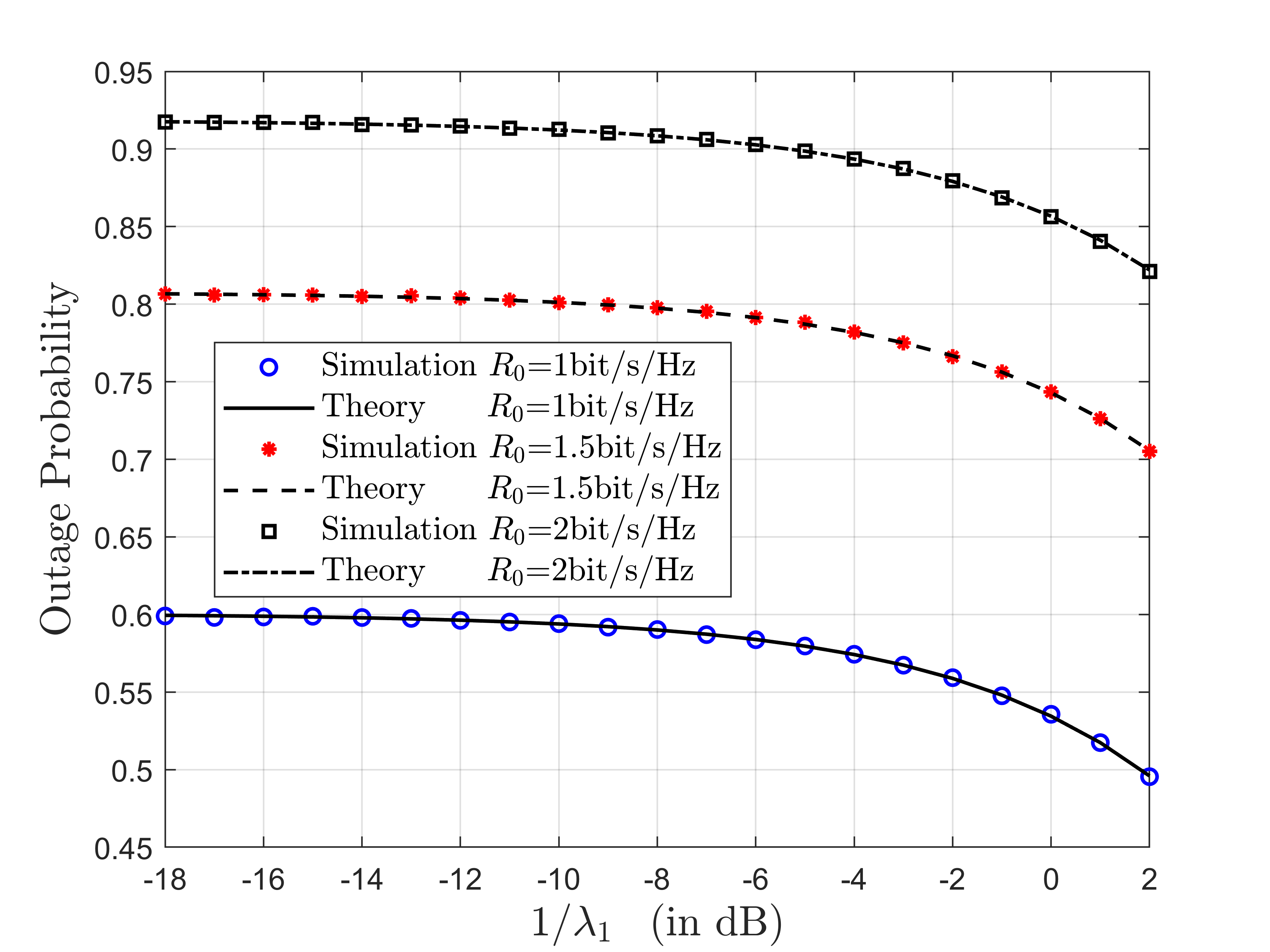
Fig. 6: Outage probability of system against relay node R​1R1 energy-harvested mean 1λ1\frac{1}{\lambda_{1}}, with parameters 1λ2=−5\frac{1}{\lambda_{2}}=-5 dB, PS=10P_{S}=10 dBm, M1=15M_{1}=15 mJ, M2=10M_{2}=10 mJ and three different data transmission rates (R0R_{0} =1, 1.5 and 2 bit/s/Hz).

Refer to caption

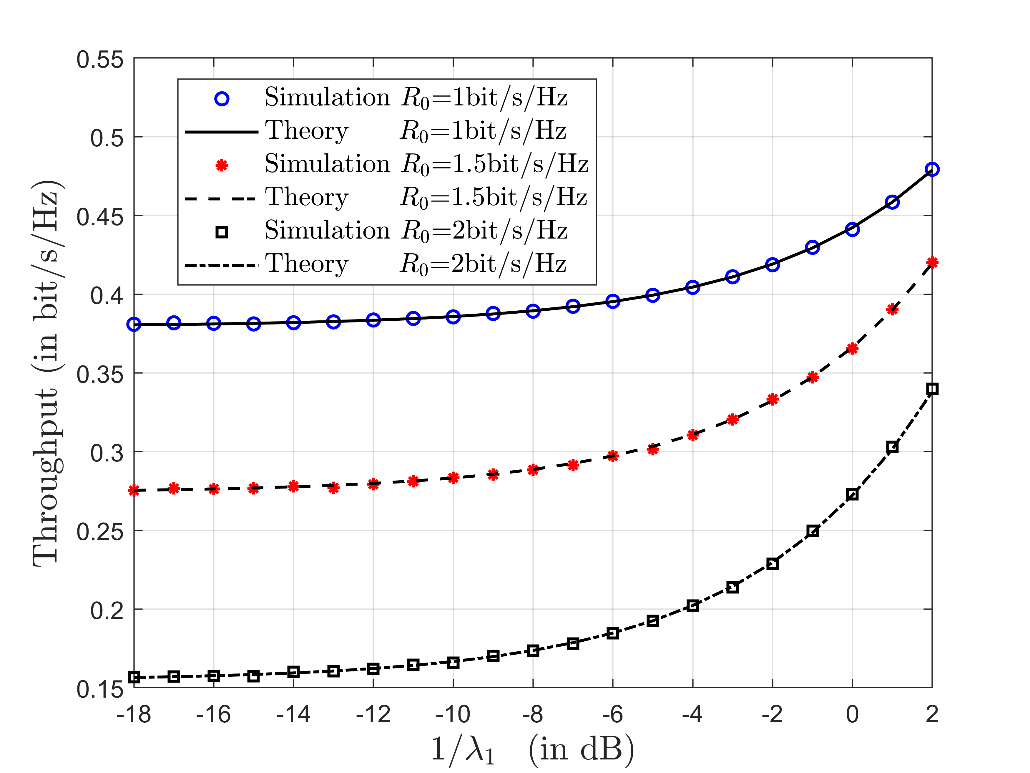
Fig. 7: Throughput of system against relay node R​1R1 energy-harvested mean 1λ1\frac{1}{\lambda_{1}}, with parameters 1λ2=−5\frac{1}{\lambda_{2}}=-5 dB, PS=10P_{S}=10 dBm, M1=15M_{1}=15 mJ, M2=10M_{2}=10 mJ, and three different data transmission rates (R0R_{0} =1, 1.5 and 2 bit/s/Hz).

Fig. 6 and Fig. 7 present the variation of system outage probability and system throughput with relay node R​1R1 energy-harvested mean 1λ1\frac{1}{\lambda_{1}} for three different data transmission rates (R0R_{0} =1, 1.5 and 2 bit/s/Hz), respectively. From Fig. 6, it can be seen that the system outage probabilities, which are obtained by simulation and theory, decrease with the increase of 1λ1\frac{1}{\lambda_{1}} under the condition that the value of R0R_{0} is fixed, on the contrary, decrease with the decrease of the value of R0R_{0} when 1λ1\frac{1}{\lambda_{1}} is fixed. In contrast, in Fig. 7, the system throughputs, which are obtained by simulation and theory, increase with the increase of 1λ1\frac{1}{\lambda_{1}} under the condition that the value of R0R_{0} is fixed, and conversely, increase with the decrease of the value of R0R_{0} when 1λ1\frac{1}{\lambda_{1}} is fixed. This is due to the fact that the increase of 1λ1\frac{1}{\lambda_{1}} may lead to the R​1R1 having more opportunities to forward the packet, and the decrease of the value of R0R_{0} would reduce the threshold Γt​h\Gamma_{th} which indicates DD may successfully receive the packet. Moreover, from Fig. 6 and Fig. 7, it can also be seen that the results obtained by theoretical analysis are consistent with the simulation, which effectively verifies the theoretical analysis of system outage probability and system throughput from variations of 1λ1\frac{1}{\lambda_{1}} and R0R_{0}.

Refer to caption

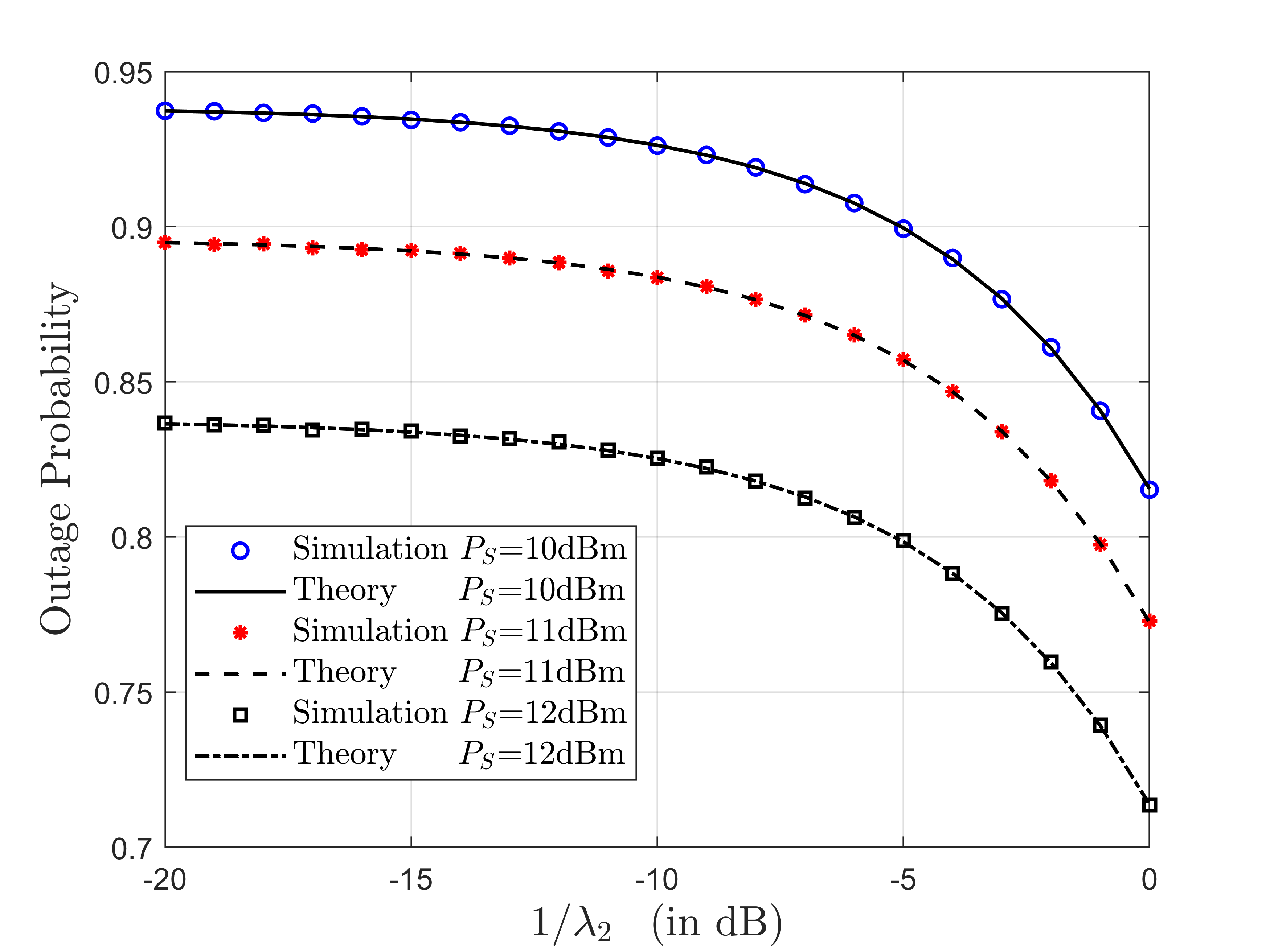
Fig. 8: Outage probability of system against relay node R​2R2 energy-harvested mean 1λ2\frac{1}{\lambda_{2}}, with parameters 1λ1=−10\frac{1}{\lambda_{1}}=-10 dB, R0=2R_{0}=2 bit/s/Hz, M1=8M_{1}=8 mJ, M2=8M_{2}=8 mJ and three different source transmit powers (PSP_{S} = 10, 11 and 12 dBm).

Refer to caption

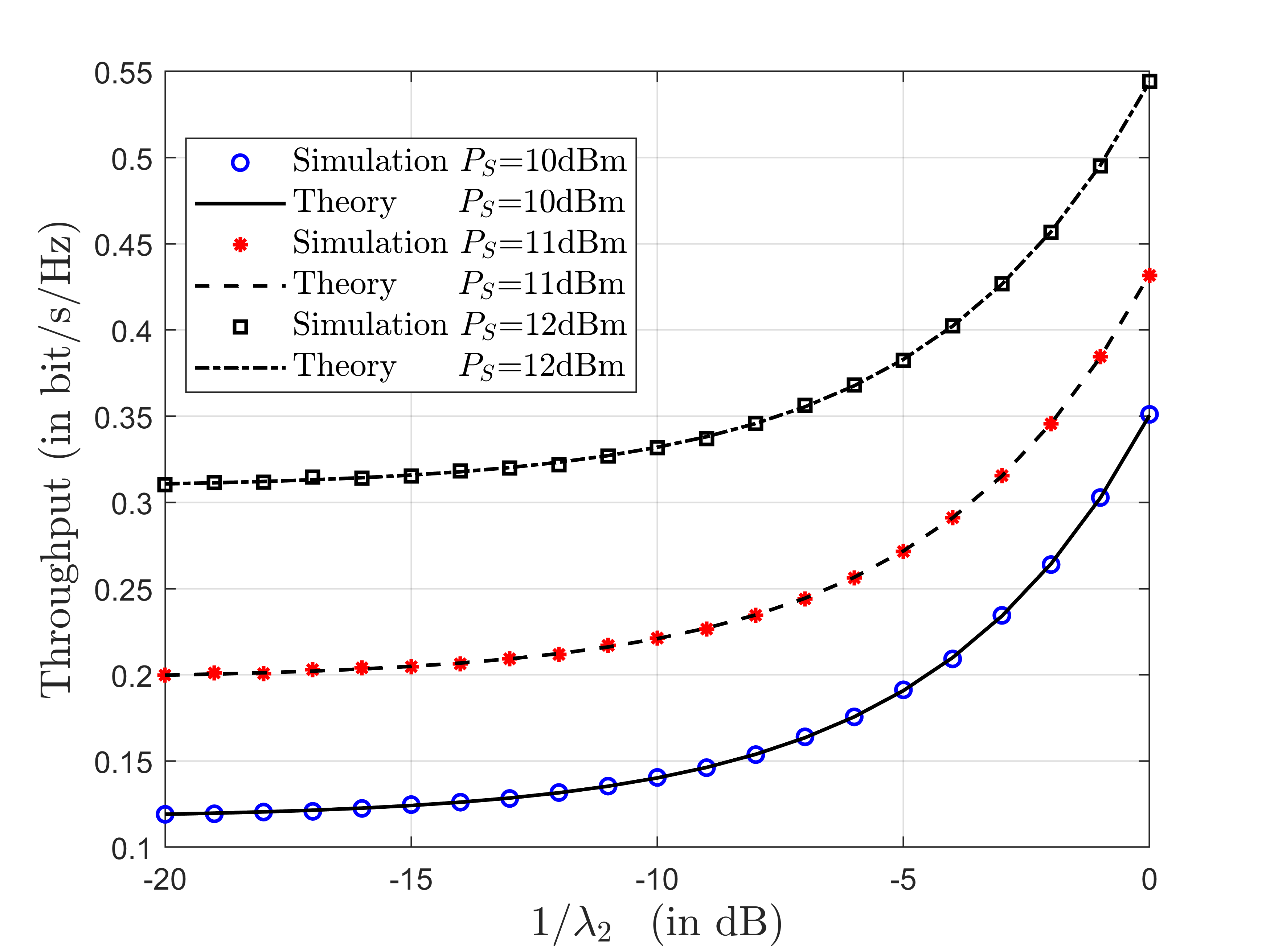
Fig. 9: Throughput of system against relay node R​2R2 energy-harvested mean 1λ2\frac{1}{\lambda_{2}}, with parameters 1λ1=−10\frac{1}{\lambda_{1}}=-10 dB, R0=2R_{0}=2 bit/s/Hz, M1=8M_{1}=8 mJ, M2=8M_{2}=8 mJ and three different source transmit powers (PSP_{S} = 10, 11 and 12 dBm).

Fig. 8 and 9 illustrate the variation of system outage probability and system throughput with relay node R​2R2 energy-harvested mean 1λ2\frac{1}{\lambda_{2}} for three different source transmit powers (PSP_{S} = 10, 11 and 12 dBm), respectively. From Fig. 8, it can be seen that the system outage probabilities, which are obtained by simulation and theory, decrease with the increase of 1λ2\frac{1}{\lambda_{2}} under the condition that the value of PSP_{S} is fixed, similarly, decrease with the increase of the value of PSP_{S} when 1λ2\frac{1}{\lambda_{2}} is fixed. However, a comparison of Fig. 8 and Fig. 9 shows that under the same parameter setting conditions, the changing trend of system throughput in Fig. 9 is opposite to that of system outage probability in Fig. 8. This results from that the increase of 1λ2\frac{1}{\lambda_{2}} and PSP_{S} may increase the probability of R​2R2 and SS to forward the packet, respectively. So that the probability of DD successfully receiving the packet increases. In addition, both Fig. 8 and Fig. 9 show that the results obtained by theoretical analysis are consistent with the simulation, which effectively verifies the theoretical analysis of system outage probability and system throughput by the variations of 1λ2\frac{1}{\lambda_{2}} and PSP_{S}.

Refer to caption

Fig. 10: Outage probability of system against source transmit power PSP_{S}, with parameters 1λ1=−6\frac{1}{\lambda_{1}}=-6 dB, 1λ2=−6\frac{1}{\lambda_{2}}=-6 dB, R0=2R_{0}=2 bit/s/Hz and three different relay energy consumptions {(M1,M2)(M_{1},M_{2}) = (8 mJ, 6 mJ), (10 mJ, 8 mJ) and (15 mJ, 13 mJ)}.

Refer to caption

Fig. 11: Throughput of system against source transmit power PSP_{S}, with parameters 1λ1=−6\frac{1}{\lambda_{1}}=-6 dB, 1λ2=−6\frac{1}{\lambda_{2}}=-6 dB, R0=2R_{0}=2 bit/s/Hz and three different relay energy consumptions {(M1,M2)(M_{1},M_{2}) = (8 mJ, 6 mJ), (10 mJ, 8 mJ) and (15 mJ, 13 mJ)}.

Fig. 10 and Fig. 11 depict the variation of system outage probability and system throughput with the source transmit power PSP_{S} for three different relay energy consumptions {(M1,M2)(M_{1},M_{2}) = (8 mJ, 6 mJ), (10 mJ, 8 mJ) and (15 mJ, 13 mJ)}, respectively. From Fig. 10, it can be seen that the system outage probabilities, which are obtained by simulation and theory, decrease with the increase of PSP_{S} under the condition that the value of (M1,M2)(M_{1},M_{2}) is fixed, on the contrary, increase with the increase of the value of (M1,M2)(M_{1},M_{2}) when PSP_{S} is fixed. Then, comparing Fig. 11 with Fig. 10, it is easy to find that under the same parameter setting conditions, the changing trend of system throughput in Fig. 11 is opposite to that of system outage probability in Fig. 10. Furthermore, it is also easy to find that when PS>10P_{S}>10 dBm, compared with relay energy consumption (M1,M2)(M_{1},M_{2}), the source transmits power PSP_{S} has a greater impact on system outage probability and system throughput. This is because with the gradual increase of source transmission power PSP_{S}, the probability of the packet directly transmitted from the source node SS to the destination node DD increases significantly. Meanwhile, it can be seen from both Fig. 10 and Fig. 11 that the theoretical results fit into the simulation results, which effectively verifies the theoretical analysis of system outage probability and system throughput from the variations of PSP_{S} and (M1,M2)(M_{1},M_{2}).

Refer to caption

Fig. 12: Outage probability of system against data transmission rate R0R_{0}, with parameters 1λ1=−7\frac{1}{\lambda_{1}}=-7 dB, 1λ2=−7\frac{1}{\lambda_{2}}=-7 dB, PS=11P_{S}=11 dBm and three different relay energy consumptions {(M1,M2)(M_{1},M_{2}) = (10 mJ, 8 mJ), (15 mJ, 13 mJ) and (25 mJ, 23 mJ)}.

Refer to caption

Fig. 13: Throughput of system against data transmission rate R0R_{0}, with parameters 1λ1=−7\frac{1}{\lambda_{1}}=-7 dB, 1λ2=−7\frac{1}{\lambda_{2}}=-7 dB, PS=11P_{S}=11 dBm and three different relay energy consumptions {(M1,M2)(M_{1},M_{2}) = (10 mJ, 8 mJ), (15 mJ, 13 mJ) and (25 mJ, 23 mJ)}.

Fig. 12 and Fig. 13 present the variation of system outage probability and system throughput with the data transmission rate R0R_{0} for three different relay energy consumptions {(M1,M2)(M_{1},M_{2}) = (10 mJ, 8 mJ), (15 mJ, 13 mJ) and (25 mJ, 23 mJ)}, respectively. From Fig. 12, it can be seen that the system outage probabilities, which are obtained by simulation and theory, increase with the increase of R0R_{0} or (M1,M2)(M_{1},M_{2}). Especially compared with relay energy consumption (M1,M2)(M_{1},M_{2}), data transmission rate R0R_{0} has a greater impact on system outage probabilities. This is due to the increase of the value of R0R_{0} would significantly increase the threshold Γt​h\Gamma_{th}, which may greatly reduce the probability of node DD successfully receiving the packet. However, from Fig. 13, it can be seen that for three different relay energy consumptions {(M1,M2)(M_{1},M_{2}) = (10 mJ, 8 mJ), (15 mJ, 13 mJ) and (25 mJ, 23 mJ)}, the system throughputs, which are obtained by simulation and theory, increase with the increase of R0R_{0} when R0<1R_{0}<1 bit/s/Hz, and conversely, decrease with the increase of R0R_{0} when the R0>1R_{0}>1 bit/s/Hz. Therefore, it can be concluded that under this system parameter setting, the optimal throughput can be obtained when R0R_{0} is about 1 bit/s/Hz. Moreover, both Fig. 12 and Fig. 13 show that the curves obtained from the theoretical analysis are consistent with the simulation values, which effectively verifies the theoretical analysis of system outage probability and system throughput from variations of R0R_{0} and (M1,M2)(M_{1},M_{2}).

Refer to caption

Fig. 14: Slope of system theoretical throughput against data transmission rate R0R_{0}, with parameters 1λ1=−7\frac{1}{\lambda_{1}}=-7 dB, 1λ2=−7\frac{1}{\lambda_{2}}=-7 dB, PS=11P_{S}=11 dBm and three different relay energy consumptions {(M1,M2)(M_{1},M_{2}) = (10 mJ, 8 mJ), (15 mJ, 13 mJ) and (25 mJ, 23 mJ)}.

Fig. 14 illustrates the variation of slope of theoretical throughput curves to data transmission rate R0R_{0} for three different relay energy consumptions {(M1,M2)(M_{1},M_{2}) = (10 mJ, 8 mJ), (15 mJ, 13 mJ) and (25 mJ, 23 mJ)}, respectively. From Fig. 14, it can be clearly observed that R0=1R_{0}=1 bit/s/Hz is approximately the point where the slopes of the three different theoretical throughput curves are zero. Moreover, the slopes corresponding to points on the left of R0=1R_{0}=1 bit/s/Hz are positive, while the slopes corresponding to points on the right of R0=1R_{0}=1 bit/s/Hz is negative. That is, when R0R_{0} is about 1 bit/s/Hz, the optimal throughput can be obtained, which is consistent with the analysis result in Fig. 13, and also effectively verifies the theoretical analysis of the system throughput.

VI Conclusion

This paper proposes the OR aided cooperative communication network with EH. Where the OR protocol is proposed to select the packet transmission path based on the node transmission priority. Additionally, the STM-based algorithm is proposed to find the probability distribution of the CBN set. Using both DCSMC model and the probability distribution, the existence conditions and analytical expressions of the limiting distribution of energy in energy buffers are determined. Then, based on the limiting distribution of energy in energy buffers, the network outage probability and throughput are analyzed, and the corresponding closed-form expressions are given. Furthermore, various simulation findings show that the simulation results are in line with the theoretical analysis results. The relay system containing more than two EH relay nodes is proposed as a future research direction.

Appendix A Proof of Theorem 1

According to the energy storage process B2​(i)B_{2}(i) with the infinite-size energy buffer in Eq. (10), the variable OR​(i)O_{R}(i) is defined by [17, Appendix B]

OR​(i)={1,ℙ220,ℙ21O_{R}(i)=\begin{cases}1,\quad\mathbb{P}_{22}\\ 0,\quad\mathbb{P}_{21}\end{cases} (53)

where ℙ21\mathbb{P}_{21} and ℙ22\mathbb{P}_{22} have been given in Eq. (11) and Eq. (12), respectively. Implying Eq. (53), the energy storage process in Eq. (10) can be re-expressed as follows

B2​(i+1)−B2​(i)=X2​(i)−M2​OR​(i).B_{2}(i+1)-B_{2}(i)=X_{2}(i)-M_{2}O_{R}(i). (54)

According to the law of large numbers, the average energy harvesting rate can be obtained as follows

𝔼⁡[X2​(i)]=limN→∞1N​∑i=1NX2​(i),\mathbb{E}[X_{2}(i)]=\lim_{N\to\infty}\frac{1}{N}\sum_{i=1}^{N}X_{2}(i), (55)

similarly, the average energy consumption rate can be given by

𝔼⁡[M2​OR​(i)]=limN→∞1N​∑i=1NM2​OR​(i)≤M2​{limN→∞1N​∑i=1NOR​(i)}.\begin{split}\mathbb{E}[M_{2}O_{R}(i)]&=\lim_{N\to\infty}\frac{1}{N}\sum_{i=1}^{N}M_{2}O_{R}(i)\\ &\leq M_{2}\Big\{\lim_{N\to\infty}\frac{1}{N}\sum_{i=1}^{N}O_{R}(i)\Big\}.\end{split} (56)

moreover,

𝔼​[OR​(i)]=limN→∞1N​∑i=1NOR​(i)=1×Pr{OR(i)=1}+0×Pr{OR(i)=0}=Pr⁡{S​(i)=s3,C9​(i)}+Pr⁡{S​(i)=s4,C9​(i)}≤(p3+p4)​(1−e−ΩS​D​Γt​h)​e−ΩR​2​D​Γt​h.\begin{split}\mathbb{E}[O_{R}(i)]&=\lim_{N\to\infty}\frac{1}{N}\sum_{i=1}^{N}O_{R}(i)\\ &=1\times\mathrm{Pr}\{O_{R}(i)=1\}+0\times\mathrm{Pr}\{O_{R}(i)=0\}\\ &=\mathrm{Pr}\{\textbf{S}(i)=\textbf{s}_{3},C_{9}(i)\}+\mathrm{Pr}\{\textbf{S}(i)=\textbf{s}_{4},C_{9}(i)\}\\ &\leq\left(p_{3}+p_{4}\right)\left(1-e^{-\Omega_{SD}\Gamma_{th}}\right)e^{-\Omega_{R2D}\Gamma_{th}}.\end{split} (57)

From Eq. (56) and Eq. (57), we obtain

𝔼⁡[M2​OR​(i)]≤M2​(p3+p4)​(1−e−ΩS​D​Γt​h)​e−ΩR​2​D​Γt​h.\begin{split}\mathbb{E}[M_{2}O_{R}(i)]&\leq M_{2}\left(p_{3}+p_{4}\right)\left(1-e^{-\Omega_{SD}\Gamma_{th}}\right)e^{-\Omega_{R2D}\Gamma_{th}}.\end{split} (58)

If ψ1≤1\psi_{1}\leq 1, from Eq. (13), we get

𝔼⁡[X2​(i)]≥M2​(p3+p4)​(1−e−ΩS​D​Γt​h)​e−ΩR​2​D​Γt​h.\begin{split}\mathbb{E}[X_{2}(i)]\geq M_{2}\left(p_{3}+p_{4}\right)\left(1-e^{-\Omega_{SD}\Gamma_{th}}\right)e^{-\Omega_{R2D}\Gamma_{th}}.\end{split} (59)

Therefore, if ψ1≤1\psi_{1}\leq 1, from Eq. (55), Eq. (56), Eq. (58) and Eq. (59), we obtain

limN→∞1N​∑i=1NX2​(i)≥limN→∞1N​∑i=1NM2​OR​(i).\lim_{N\to\infty}\frac{1}{N}\sum_{i=1}^{N}X_{2}(i)\geq\lim_{N\to\infty}\frac{1}{N}\sum_{i=1}^{N}M_{2}O_{R}(i). (60)

According to Eq. (54) and Eq. (60), we have

limN→∞1N​∑i=1NB2​(i+1)≥limN→∞1N​∑i=1NB2​(i).\lim_{N\to\infty}\frac{1}{N}\sum_{i=1}^{N}B_{2}(i+1)\geq\lim_{N\to\infty}\frac{1}{N}\sum_{i=1}^{N}B_{2}(i). (61)

Clearly, if the inequality condition holds in Eq. (61), the comparison of between B2​(i+1)B_{2}(i+1) and B2​(i)B_{2}(i) shows that the energy accumulates in the buffer over time slot, i.e., limi→∞𝔼⁡[B2​(i)]=∞\begin{matrix}\lim_{i\to\infty}\mathbb{E}[B_{2}(i)]=\infty\end{matrix}. Therefore, the stationary distribution of B2​(i)B_{2}(i) does not exist, and after a finite number of time slots, B2​(i)>M2B_{2}(i)>M_{2} almost always hold [7, Appendix A]. In addition, if the equality condition holds in Eq. (60), according to Eq. (60) and Eq. (56), we get

limN→∞1N​∑i=1NX2​(i)=limN→∞1N​∑i=1NM2​OR​(i).\lim_{N\to\infty}\frac{1}{N}\sum_{i=1}^{N}X_{2}(i)=\lim_{N\to\infty}\frac{1}{N}\sum_{i=1}^{N}M_{2}O_{R}(i). (62)

Eq. (62) indicates that in the energy buffer with the DCSMC model, the average energy harvesting rate equals the average energy consumption rate, which is unstable [33]. Therefore, the buffer may almost always provide M2M_{2} amount of energy.

Appendix B Proof of Theorem 2

According to the total probability theorem, ℙ21\mathbb{P}_{21} and ℙ22\mathbb{P}_{22} together constitutes a complete set of events accompanying event B2​(i+1)B_{2}(i+1). Therefore, the cumulative distribution function (CDF) of B2​(i+1)B_{2}(i+1) in storage process in Eq. (10) may be evaluated as follows [17, Appendix C]

Pr{B2(i+1)≤x}=Pr{B2(i)+X2(i)≤x,S(i)=s1}+Pr{B2(i)+X2(i)≤x,S(i)=s2}+Pr{B2(i)+X2(i)≤x,S(i)=s3,C1(i)}+Pr{B2(i)+X2(i)≤x,S(i)=s3,C1¯(i),B2(i)<M2}+Pr{B2(i)+X2(i)≤x,S(i)=s3,C1¯(i),B2(i)≥M2,γR​2​D(i)<Γt​h}+Pr{B2(i)+X2(i)≤x,S(i)=s4,C1(i)}+Pr{B2(i)+X2(i)≤x,S(i)=s4,C1¯(i),B2(i)<M2}+Pr{B2(i)+X2(i)≤x,S(i)=s4,C1¯(i),B2(i)≥M2,γR​2​D(i)<Γt​h}+Pr{B2(i)+X2(i)−M2≤x,S(i)=s3,C9(i)}+Pr{B2(i)+X2(i)−M2≤x,S(i)=s4,C9(i)}.\begin{split}&\mathrm{Pr}\{B_{2}(i+1)\leq x\}\\ &\quad=\mathrm{Pr}\{B_{2}(i)+X_{2}(i)\leq x,\textbf{S}(i)=\textbf{s}_{1}\}\\ &\quad+\mathrm{Pr}\{B_{2}(i)+X_{2}(i)\leq x,\textbf{S}(i)=\textbf{s}_{2}\}\\ &\quad+\mathrm{Pr}\{B_{2}(i)+X_{2}(i)\leq x,\textbf{S}(i)=\textbf{s}_{3},C_{1}(i)\}\\ &\quad+\mathrm{Pr}\{B_{2}(i)+X_{2}(i)\leq x,\textbf{S}(i)=\textbf{s}_{3},\overline{C_{1}}(i),B_{2}(i)<M_{2}\}\\ &\quad+\mathrm{Pr}\{B_{2}(i)+X_{2}(i)\leq x,\textbf{S}(i)=\textbf{s}_{3},\overline{C_{1}}(i),B_{2}(i)\geq M_{2},\\ &\quad\gamma_{R2D}(i)<\Gamma_{th}\}\\ &\quad+\mathrm{Pr}\{B_{2}(i)+X_{2}(i)\leq x,\textbf{S}(i)=\textbf{s}_{4},C_{1}(i)\}\\ &\quad+\mathrm{Pr}\{B_{2}(i)+X_{2}(i)\leq x,\textbf{S}(i)=\textbf{s}_{4},\overline{C_{1}}(i),B_{2}(i)<M_{2}\}\\ &\quad+\mathrm{Pr}\{B_{2}(i)+X_{2}(i)\leq x,\textbf{S}(i)=\textbf{s}_{4},\overline{C_{1}}(i),B_{2}(i)\geq M_{2},\\ &\quad\gamma_{R2D}(i)<\Gamma_{th}\}\\ &\quad+\mathrm{Pr}\{B_{2}(i)+X_{2}(i)-M_{2}\leq x,\textbf{S}(i)=\textbf{s}_{3},C_{9}(i)\}\\ &\quad+\mathrm{Pr}\{B_{2}(i)+X_{2}(i)-M_{2}\leq x,\textbf{S}(i)=\textbf{s}_{4},C_{9}(i)\}.\end{split} (63)

Let B2​(i)=μ2B_{2}(i)=\mu_{2}, X2​(i)=X2X_{2}(i)=X_{2}, S​(i)=S\textbf{S}(i)=\textbf{S}, C1​(i)=C1C_{1}(i)=C_{1}, C1¯​(i)=C1¯\overline{C_{1}}(i)=\overline{C_{1}}, C9​(i)=C9C_{9}(i)=C_{9}, and γR​2​D​(i)=γR​2​D\gamma_{R2D}(i)=\gamma_{R2D}. Eq. (63) may be presented by

Pr{B2(i+1)≤x}=Pr{μ2+X2≤x,S=s1}+Pr{μ2+X2≤x,S=s2}+Pr{μ2+X2≤x,S=s3,C1}+Pr{μ2+X2≤x,S=s3,C1¯,B2(i)<M2}+Pr{μ2+X2≤x,S=s3,C1¯,B2≥M2,γR​2​D<Γt​h}+Pr{μ2+X2≤x,S=s4,C1}+Pr{μ2+X2≤x,S=s4,C1¯,μ2<M2}+Pr{μ2+X2≤x,S=s4,C1¯,μ2≥M2,γR​2​D<Γt​h}+Pr{μ2+X2−M2≤x,S=s3,C9}+Pr{μ2+X2−M2≤x,S=s4,C9}.\begin{split}&\mathrm{Pr}\{B_{2}(i+1)\leq x\}\\ &\quad=\mathrm{Pr}\{\mu_{2}+X_{2}\leq x,\textbf{S}=\textbf{s}_{1}\}\\ &\quad+\mathrm{Pr}\{\mu_{2}+X_{2}\leq x,\textbf{S}=\textbf{s}_{2}\}\\ &\quad+\mathrm{Pr}\{\mu_{2}+X_{2}\leq x,\textbf{S}=\textbf{s}_{3},C_{1}\}\\ &\quad+\mathrm{Pr}\{\mu_{2}+X_{2}\leq x,\textbf{S}=\textbf{s}_{3},\overline{C_{1}},B_{2}(i)<M_{2}\}\\ &\quad+\mathrm{Pr}\{\mu_{2}+X_{2}\leq x,\textbf{S}=\textbf{s}_{3},\overline{C_{1}},B_{2}\geq M_{2},\gamma_{R2D}<\Gamma_{th}\}\\ &\quad+\mathrm{Pr}\{\mu_{2}+X_{2}\leq x,\textbf{S}=\textbf{s}_{4},C_{1}\}\\ &\quad+\mathrm{Pr}\{\mu_{2}+X_{2}\leq x,\textbf{S}=\textbf{s}_{4},\overline{C_{1}},\mu_{2}<M_{2}\}\\ &\quad+\mathrm{Pr}\{\mu_{2}+X_{2}\leq x,\textbf{S}=\textbf{s}_{4},\overline{C_{1}},\mu_{2}\geq M_{2},\gamma_{R2D}<\Gamma_{th}\}\\ &\quad+\mathrm{Pr}\{\mu_{2}+X_{2}-M_{2}\leq x,\textbf{S}=\textbf{s}_{3},C_{9}\}\\ &\quad+\mathrm{Pr}\{\mu_{2}+X_{2}-M_{2}\leq x,\textbf{S}=\textbf{s}_{4},C_{9}\}.\end{split} (64)

Denote G2i+1​(x)G^{i+1}_{2}(x) as the CDF of B2​(i+1)B_{2}(i+1), namely, Pr{B2(i+1)≤x}=G2i+1(x)\mathrm{Pr}\{B_{2}(i+1)\leq x\}=G^{i+1}_{2}(x). When i→∞i\to\infty, if the buffer reaches its steady state, it follows that, Pr{B2(i+1)≤x}=G2i+1(x)=G2i(x)=G2(x)\mathrm{Pr}\{B_{2}(i+1)\leq x\}=G^{i+1}_{2}(x)=G^{i}_{2}(x)=G_{2}(x). In this state, Eq. (64) may be written as follows

G2​(x)=(p1+p2)​∫μ2=0xFX2​(x−μ2)​g2​(μ2)​d​μ2+(p3+p4)∫r1=Γt​h∞∫μ2=0xFX2(x−μ2)g2(μ2)×fγS​D​(r1)​d​μ2​d​r1+(p3+p4)∫r1=0Γt​h∫μ2=0m​i​n​(x,M2)FX2(x−μ2)g2(μ2)×fγS​D​(r1)​d​μ2​d​r1+(p3+p4)∫r1=0Γt​h∫r2=0Γt​h∫μ2=M2xFX2(x−μ2)g2(μ2)×fγS​D​(r1)​fγR​2​D​(r2)​d​μ2​d​r1​d​r2+(p3+p4)∫r1=0Γt​h∫r2=Γt​h∞∫μ2=M2x+M2FX2(x+M2−μ2)×g2​(μ2)​fγS​D​(r1)​fγR​2​D​(r2)​d​μ2​d​r1​d​r2,\begin{split}G_{2}(x)&=(p_{1}+p_{2})\int_{\mu_{2}=0}^{x}F_{X_{2}}(x-\mu_{2})g_{2}(\mu_{2})\,d\mu_{2}\\ &+(p_{3}+p_{4})\int_{r_{1}=\Gamma_{th}}^{\infty}\int_{\mu_{2}=0}^{x}F_{X_{2}}(x-\mu_{2})g_{2}(\mu_{2})\\ &\times f_{\gamma_{SD}}(r_{1})\,d\mu_{2}\,dr_{1}\\ &+(p_{3}+p_{4})\int_{r_{1}=0}^{\Gamma_{th}}\int_{\mu_{2}=0}^{min(x,M_{2})}F_{X_{2}}(x-\mu_{2})g_{2}(\mu_{2})\\ &\times f_{\gamma_{SD}}(r_{1})\,d\mu_{2}\,dr_{1}\\ &+(p_{3}+p_{4})\int_{r_{1}=0}^{\Gamma_{th}}\int_{r_{2}=0}^{\Gamma_{th}}\int_{\mu_{2}=M_{2}}^{x}F_{X_{2}}(x-\mu_{2})g_{2}(\mu_{2})\\ &\times f_{\gamma_{SD}}(r_{1})f_{\gamma_{R2D}}(r_{2})\,d\mu_{2}\,dr_{1}\,dr_{2}\\ &+(p_{3}+p_{4})\int_{r_{1}=0}^{\Gamma_{th}}\int_{r_{2}=\Gamma_{th}}^{\infty}\int_{\mu_{2}=M_{2}}^{x+M_{2}}F_{X_{2}}(x+M_{2}-\mu_{2})\\ &\times g_{2}(\mu_{2})f_{\gamma_{SD}}(r_{1})f_{\gamma_{R2D}}(r_{2})\,d\mu_{2}\,dr_{1}\,dr_{2},\end{split} (65)

where FX2​(x)=1−e−λ2​xF_{X_{2}}(x)=1-e^{-\lambda_{2}x} is the CDF of X2X_{2}. g2​(x)g_{2}(x) is the derivative of G2​(x)G_{2}(x). In addition, fγS​D​(r1)=ΩS​D​e−ΩS​D​r1f_{\gamma_{SD}}(r_{1})=\Omega_{SD}e^{-\Omega_{SD}r_{1}} and fγR​2​D​(r2)=ΩR​2​D​e−ΩR​2​D​r2f_{\gamma_{R2D}}(r_{2})=\Omega_{R2D}e^{-\Omega_{R2D}r_{2}} are the PDFs of γS​D\gamma_{SD} and γR​2​D\gamma_{R2D}, respectively. Substituting fγS​D​(r1)f_{\gamma_{SD}}(r_{1}) and fγR​2​D​(r2)f_{\gamma_{R2D}}(r_{2}) in Eq. (65), and simplifying Eq. (65), we arrive at

G2​(x)={G21​(x),0≤x<M2G22​(x),x≥M2G_{2}(x)=\begin{cases}G_{21}(x),&0\leq x<M_{2}\\ G_{22}(x),&x\geq M_{2}\end{cases} (66)

where,

G21​(x)=∫μ2=0xFX2​(x−μ2)​g2​(μ2)​d​μ2+(p3+p4)​(1−e−ΩS​D​Γt​h)​e−ΩR​2​D​Γt​h×∫μ2=M2x+M2FX2​(x+M2−μ2)​g2​(μ2)​d​μ2,\begin{split}G_{21}(x)&=\int_{\mu_{2}=0}^{x}F_{X_{2}}(x-\mu_{2})g_{2}(\mu_{2})\,d\mu_{2}\\ &+(p_{3}+p_{4})\left(1-e^{-\Omega_{SD}\Gamma_{th}}\right)e^{-\Omega_{R2D}\Gamma_{th}}\\ &\times\int_{\mu_{2}=M_{2}}^{x+M_{2}}F_{X_{2}}(x+M_{2}-\mu_{2})g_{2}(\mu_{2})\,d\mu_{2},\end{split} (67)
G22​(x)=∫μ2=0M2FX2​(x−μ2)​g2​(μ2)​d​μ2+[1−(p3+p4)​(1−e−ΩS​D​Γt​h)​e−ΩR​2​D​Γt​h]×∫μ2=M2xFX2​(x−μ2)​g2​(μ2)​d​μ2+[(p3+p4)​(1−e−ΩS​D​Γt​h)​e−ΩR​2​D​Γt​h]×∫μ2=M2x+M2FX2​(x+M2−μ2)​g2​(μ2)​d​μ2.\begin{split}G_{22}(x)&=\int_{\mu_{2}=0}^{M_{2}}F_{X_{2}}(x-\mu_{2})g_{2}(\mu_{2})\,d\mu_{2}\\ &+\left[1-\left(p_{3}+p_{4}\right)\left(1-e^{-\Omega_{SD}\Gamma_{th}}\right)e^{-\Omega_{R2D}\Gamma_{th}}\right]\\ &\times\int_{\mu_{2}=M_{2}}^{x}F_{X_{2}}(x-\mu_{2})g_{2}(\mu_{2})\,d\mu_{2}\\ &+\left[\left(p_{3}+p_{4}\right)\left(1-e^{-\Omega_{SD}\Gamma_{th}}\right)e^{-\Omega_{R2D}\Gamma_{th}}\right]\\ &\times\int_{\mu_{2}=M_{2}}^{x+M_{2}}F_{X_{2}}(x+M_{2}-\mu_{2})g_{2}(\mu_{2})\,d\mu_{2}.\end{split} (68)

According to Eq. (66), the PDF g2​(x)g_{2}(x) may be defined as

g2​(x)={g21​(x),0≤x<M2g22​(x),x≥M2.g_{2}(x)=\begin{cases}g_{21}(x),&0\leq x<M_{2}\\ g_{22}(x),&x\geq M_{2}.\end{cases} (69)

After substituting Eq. (69) into Eq. (68), the derivatives about xx on both sides of Eq. (68) may be obtained

g22​(x)=∫μ2=0M2fX2​(x−μ2)​g21​(μ2)​d​μ2+a2∫μ2=M2xfX2(x−μ2)g22(μ2)dμ2+b2∫μ2=M2x+M2fX2(x+M2−μ2)g22(μ2)dμ2,\begin{split}g_{22}(x)&=\int_{\mu_{2}=0}^{M_{2}}f_{X_{2}}(x-\mu_{2})g_{21}(\mu_{2})\,d\mu_{2}\\ &\quad+a_{2}\int_{\mu_{2}=M_{2}}^{x}f_{X_{2}}(x-\mu_{2})g_{22}(\mu_{2})\,d\mu_{2}\\ &\quad+b_{2}\int_{\mu_{2}=M_{2}}^{x+M_{2}}f_{X_{2}}(x+M_{2}-\mu_{2})g_{22}(\mu_{2})\,d\mu_{2},\end{split} (70)

where,

a2=[1−(p3+p4)​(1−e−ΩS​D​Γt​h)​e−ΩR​2​D​Γt​h],a_{2}=\left[1-\left(p_{3}+p_{4}\right)\left(1-e^{-\Omega_{SD}\Gamma_{th}}\right)e^{-\Omega_{R2D}\Gamma_{th}}\right], (71)
b2=[(p3+p4)​(1−e−ΩS​D​Γt​h)​e−ΩR​2​D​Γt​h].b_{2}=\left[\left(p_{3}+p_{4}\right)\left(1-e^{-\Omega_{SD}\Gamma_{th}}\right)e^{-\Omega_{R2D}\Gamma_{th}}\right]. (72)

Clearly, a2+b2=1a_{2}+b_{2}=1. Furthermore, there is evidence that storage process in Eq. (10) possesses a unique stationary distribution [7, Appendix B], when M2>𝔼⁡[X2​(i)]=1/λ2M_{2}>\mathbb{E}[X_{2}(i)]=1/\lambda_{2}. In other words, g2​(x)g_{2}(x) has unique solution. Furthermore, g22​(x)g_{22}(x) be assumed to have an exponential-type solution expressed by g22​(x)=k2​eQ2​xg_{22}(x)=k_{2}e^{Q_{2}x} [7, Appendix C]. Substituting g22​(x)=k2​eQ2​xg_{22}(x)=k_{2}e^{Q_{2}x} and fX2​(x)=λ2​e−λ2​xf_{X_{2}}(x)=\lambda_{2}e^{-\lambda_{2}x} into Eq. (70), we obtain

k2​eQ2​x=∫μ2=0M2λ2​e−λ2​(x−μ2)​g21​(μ2)​d​μ2+a2∫μ2=M2xλ2e−λ2​(x−μ2)k2eQ2​μ2dμ2+b2∫μ2=M2x+M2λ2e−λ2​(x+M2−μ2)k2eQ2​μ2dμ2.\begin{split}k_{2}e^{Q_{2}x}&=\int_{\mu_{2}=0}^{M_{2}}\lambda_{2}e^{-\lambda_{2}(x-\mu_{2})}g_{21}(\mu_{2})\,d\mu_{2}\\ &\quad+a_{2}\int_{\mu_{2}=M_{2}}^{x}\lambda_{2}e^{-\lambda_{2}(x-\mu_{2})}k_{2}e^{Q_{2}\mu_{2}}\,d\mu_{2}\\ &\quad+b_{2}\int_{\mu_{2}=M_{2}}^{x+M_{2}}\lambda_{2}e^{-\lambda_{2}(x+M_{2}-\mu_{2})}k_{2}e^{Q_{2}\mu_{2}}\,d\mu_{2}.\end{split} (73)

Simplifying Eq. (73), we have

k2​eQ2​x=λ2​e−λ2​x​∫μ2=0M2eλ2​μ2​g21​(μ2)​d​μ2−λ2​k2​[b2+a2​eλ2​M2]λ2+Q2​e(Q2​M2−λ2​x)+b2​λ2​eQ2​M2+a2​λ2λ2+Q2​k2​eQ2​x.\begin{split}k_{2}e^{Q_{2}x}&=\lambda_{2}e^{-\lambda_{2}x}\int_{\mu_{2}=0}^{M_{2}}e^{\lambda_{2}\mu_{2}}g_{21}(\mu_{2})\,d\mu_{2}\\ &\quad-\dfrac{\lambda_{2}k_{2}\left[b_{2}+a_{2}e^{\lambda_{2}M_{2}}\right]}{\lambda_{2}+Q_{2}}e^{\left(Q_{2}M_{2}-\lambda_{2}x\right)}\\ &\quad+\dfrac{b_{2}\lambda_{2}e^{Q_{2}M_{2}}+a_{2}\lambda_{2}}{\lambda_{2}+Q_{2}}k_{2}e^{Q_{2}x}.\end{split} (74)

For the correctness of postulating g22​(x)=k2​eQ2​xg_{22}(x)=k_{2}e^{Q_{2}x}, both sides of Eq. (74) must be equal. Hence ,we get

b2​λ2​eQ2​M2+a2​λ2λ2+Q2=1,\displaystyle\dfrac{b_{2}\lambda_{2}e^{Q_{2}M_{2}}+a_{2}\lambda_{2}}{\lambda_{2}+Q_{2}}=1, (75a)
k2​eQ2​M2​[b2+a2​eλ2​M2]λ2+Q2=∫μ2=0M2eλ2​μ2​g21​(μ2)​d​μ2.\displaystyle\dfrac{k_{2}e^{Q_{2}M_{2}}\left[b_{2}+a_{2}e^{\lambda_{2}M_{2}}\right]}{\lambda_{2}+Q_{2}}=\int_{\mu_{2}=0}^{M_{2}}e^{\lambda_{2}\mu_{2}}g_{21}(\mu_{2})\,d\mu_{2}. (75b)

It can be seen from Eq. (75a) that Q20=0Q_{2_{0}}=0 is one of the solutions of Q2Q_{2} in Eq. (75a), but this solution does not meet the condition that g22​(x)g_{22}(x) is a finite distribution. Additionally, the other solution Q21Q_{2_{1}} of Q2Q_{2} in Eq. (75a) can be obtained by simplifying Eq. (75a) as

b2​λ2​eQ2​M2=λ2−a2​λ2+Q2=b2​λ2+Q2.b_{2}\lambda_{2}e^{Q_{2}M_{2}}=\lambda_{2}-a_{2}\lambda_{2}+Q_{2}=b_{2}\lambda_{2}+Q_{2}. (76)

Using Lambert W function, the solution Q21Q_{2_{1}} of Q2Q_{2} can be obtained as follows

Q21=−W⁡(−b2​λ2​M2​e−b2​λ2​M2)M2−b2​λ2.Q_{2_{1}}=\frac{-W\left(-b_{2}\lambda_{2}M_{2}e^{-b_{2}\lambda_{2}M_{2}}\right)}{M_{2}}-b_{2}\lambda_{2}. (77)

According to the property of Lambert W function, when b2​λ2​M2≤1b_{2}\lambda_{2}M_{2}\leq 1, W⁡(−b2​λ2​M2​e−b2​λ2​M2)=−b2​λ2​M2W\left(-b_{2}\lambda_{2}M_{2}e^{-b_{2}\lambda_{2}M_{2}}\right)=-b_{2}\lambda_{2}M_{2} so that Q21=Q20=0Q_{2_{1}}=Q_{2_{0}}=0. On the contrary, when b2​λ2​M2>1b_{2}\lambda_{2}M_{2}>1, W⁡(−b2​λ2​M2​e−b2​λ2​M2)>−b2​λ2​M2W\left(-b_{2}\lambda_{2}M_{2}e^{-b_{2}\lambda_{2}M_{2}}\right)>-b_{2}\lambda_{2}M_{2} so that Q21<0Q_{2_{1}}<0, ensuring the finite distribution of g22​(x)g_{22}(x). Thus, for the stationary distribution of g22​(x)g_{22}(x), we obtain

Q2=−W⁡(−b2​λ2​M2​e−b2​λ2​M2)M2−b2​λ2,b2​λ2​M2>1.Q_{2}=\frac{-W\left(-b_{2}\lambda_{2}M_{2}e^{-b_{2}\lambda_{2}M_{2}}\right)}{M_{2}}-b_{2}\lambda_{2},\quad b_{2}\lambda_{2}M_{2}>1. (78)

Similarly, when 0≤x<M20\leq x<M_{2}, substituting Eq. (69) into Eq. (67), the derivatives about xx on both sides of Eq. (67) can be obtained

g21​(x)=b2​∫μ2=M2x+M2fX2​(x+M2−μ2)​g22​(μ2)​d​μ2+∫μ2=0xfX2(x−μ2)g21(μ2)dμ2.\begin{split}g_{21}(x)&=b_{2}\int_{\mu_{2}=M_{2}}^{x+M_{2}}f_{X_{2}}(x+M_{2}-\mu_{2})g_{22}(\mu_{2})\,d\mu_{2}\\ &\quad+\int_{\mu_{2}=0}^{x}f_{X_{2}}(x-\mu_{2})g_{21}(\mu_{2})\,d\mu_{2}.\end{split} (79)

Substituting g22​(x)=k2​eQ2​xg_{22}(x)=k_{2}e^{Q_{2}x} and fX2​(x)=λ2​e−λ2​xf_{X_{2}}(x)=\lambda_{2}e^{-\lambda_{2}x} into Eq. (79), we get

g21​(x)=λ2​∫μ2=0xe−λ2​(x−μ2)​g21​(μ2)​d​μ2+b2​k2​λ2​eQ2​M2λ2+Q2​(eQ2​x−e−λ2​x).\begin{split}g_{21}(x)&=\lambda_{2}\int_{\mu_{2}=0}^{x}e^{-\lambda_{2}\left(x-\mu_{2}\right)}g_{21}(\mu_{2})\,d\mu_{2}\\ &\quad+\dfrac{b_{2}k_{2}\lambda_{2}e^{Q_{2}M_{2}}}{\lambda_{2}+Q_{2}}\left(e^{Q_{2}x}-e^{-\lambda_{2}x}\right).\end{split} (80)

Let r2​(x)=b2​k2​λ2​eQ2​M2λ2+Q2​(eQ2​x−e−λ2​x)r_{2}(x)=\frac{b_{2}k_{2}\lambda_{2}e^{Q_{2}M_{2}}}{\lambda_{2}+Q_{2}}\left(e^{Q_{2}x}-e^{-\lambda_{2}x}\right), and the integral equation in Eq. (80) can be rewritten as follows

g21​(x)=λ2​∫μ2=0xe−λ2​(x−μ2)​g21​(μ2)​d​μ2+r2​(x).\begin{split}g_{21}(x)=\lambda_{2}\int_{\mu_{2}=0}^{x}e^{-\lambda_{2}\left(x-\mu_{2}\right)}g_{21}(\mu_{2})\,d\mu_{2}+r_{2}(x).\end{split} (81)

Clearly, Eq. (81) is a Volterra integral equation of the second kind, whose solution is given by [6], [17] and [34, eq. 2.2.1]

g21​(x)=r2​(x)+λ2​∫t=0xr2​(t)​dt.\begin{split}g_{21}(x)=r_{2}(x)+\lambda_{2}\int_{t=0}^{x}r_{2}(t)\,dt.\end{split} (82)

Substituting r2​(x)r_{2}(x) into Eq. (82), we obtain

g21​(x)=b2​k2​λ2​eQ2​M2λ2+Q2​(eQ2​x−e−λ2​x)+λ2∫t=0xb2​k2​λ2​eQ2​M2λ2+Q2(eQ2​t−e−λ2​t)dt=b2​k2​λ2​eQ2​M2​(eQ2​x−1)Q2.\begin{split}g_{21}(x)&=\dfrac{b_{2}k_{2}\lambda_{2}e^{Q_{2}M_{2}}}{\lambda_{2}+Q_{2}}\left(e^{Q_{2}x}-e^{-\lambda_{2}x}\right)\\ &\quad+\lambda_{2}\int_{t=0}^{x}\frac{b_{2}k_{2}\lambda_{2}e^{Q_{2}M_{2}}}{\lambda_{2}+Q_{2}}\left(e^{Q_{2}t}-e^{-\lambda_{2}t}\right)\,dt\\ &=\dfrac{b_{2}k_{2}\lambda_{2}e^{Q_{2}M_{2}}\left(e^{Q_{2}x}-1\right)}{Q_{2}}.\end{split} (83)

According to the unit area condition on g2​(x)g_{2}(x), we have

∫x=0∞g2​(x)​𝑑x=∫x=0M2g21​(x)​𝑑x+∫x=M2∞g22​(x)​𝑑x=1.\int_{x=0}^{\infty}g_{2}(x)\,dx=\int_{x=0}^{M_{2}}g_{21}(x)\,dx+\int_{x=M_{2}}^{\infty}g_{22}(x)\,dx=1. (84)

Substituting g21​(x)=b2​k2​λ2​eQ2​M2​(eQ2​x−1)Q2g_{21}(x)=\frac{b_{2}k_{2}\lambda_{2}e^{Q_{2}M_{2}}\left(e^{Q_{2}x}-1\right)}{Q_{2}} and g22​(x)=k2​eQ2​xg_{22}(x)=k_{2}e^{Q_{2}x} into Eq. (84), we get

b2​k2​λ2​eQ2​M2Q2​∫x=0M2(eQ2​x−1)​𝑑x+k2​∫x=M2∞eQ2​x​𝑑x=1.\dfrac{b_{2}k_{2}\lambda_{2}e^{Q_{2}M_{2}}}{Q_{2}}\int_{x=0}^{M_{2}}\left(e^{Q_{2}x}-1\right)\,dx+k_{2}\int_{x=M_{2}}^{\infty}e^{Q_{2}x}\,dx=1. (85)

Simplifying Eq. (85), we have

b2​k2​λ​eQ2​M2Q2​[eQ2​M2−1Q2−M2]−k2​eQ2​M2Q2=1.\dfrac{b_{2}k_{2}\lambda e^{Q_{2}M_{2}}}{Q_{2}}\left[\dfrac{e^{Q_{2}M_{2}}-1}{Q_{2}}-M_{2}\right]-\dfrac{k_{2}e^{Q_{2}M_{2}}}{Q_{2}}=1. (86)

Substituting Eq. (76) into Eq. (86), then simplifying Eq. (86), the value of k2k_{2} can be obtained as follows

k2=−Q2M2​(b2​λ2+Q2).k_{2}=\dfrac{-Q_{2}}{M_{2}\left(b_{2}\lambda_{2}+Q_{2}\right)}. (87)

Substituting Eq. (76) and Eq. (87) into Eq. (83), we arrive at

g21​(x)=1−eQ2​xM2.g_{21}(x)=\dfrac{1-e^{Q_{2}x}}{M_{2}}. (88)

Substituting Eq. (88) into the right side of Eq. (75b), we obtain

∫μ2=0M2eλ2​μ2​g21​(μ2)​d​μ2=∫μ2=0M2(1−eQ2​x)​eλ2​μ2M2​d​μ2=1−e(λ2+Q2)​M2(λ2+Q2)​M2−1−eλ2​M2λ2​M2.\begin{split}\int_{\mu_{2}=0}^{M_{2}}e^{\lambda_{2}\mu_{2}}g_{21}(\mu_{2})\,d\mu_{2}&=\int_{\mu_{2}=0}^{M_{2}}\dfrac{\left(1-e^{Q_{2}x}\right)e^{\lambda_{2}\mu_{2}}}{M_{2}}\,d\mu_{2}\\ &=\dfrac{1-e^{\left(\lambda_{2}+Q_{2}\right)M_{2}}}{\left(\lambda_{2}+Q_{2}\right)M_{2}}-\dfrac{1-e^{\lambda_{2}M_{2}}}{\lambda_{2}M_{2}}.\end{split} (89)

The equation in Eq. (76) leads us to conclude λ2​M2=(λ2+Q2)​M2b2​eQ2​M2+a2\lambda_{2}M_{2}=\frac{\left(\lambda_{2}+Q_{2}\right)M_{2}}{b_{2}e^{Q_{2}M_{2}}+a_{2}}. Substituting this conclusion in Eq. (89), we have

∫μ2=0M2eλ2​μ2​g21​(μ2)​d​μ2=(1−eQ2​M2)​(b2+a2​eλ2​M2)(λ2+Q2)​M2.\begin{split}\int_{\mu_{2}=0}^{M_{2}}e^{\lambda_{2}\mu_{2}}g_{21}(\mu_{2})\,d\mu_{2}=\dfrac{\left(1-e^{Q_{2}M_{2}}\right)\left(b_{2}+a_{2}e^{\lambda_{2}M_{2}}\right)}{\left(\lambda_{2}+Q_{2}\right)M_{2}}.\end{split} (90)

Similarly, the conclude 1−eQ2​M2=−Q2b2​λ21-e^{Q_{2}M_{2}}=\frac{-Q_{2}}{b_{2}\lambda_{2}} may be obtained from Eq. (76). Substituting this conclusion in Eq. (90), we arrive at

∫μ2=0M2eλ2​μ2​g21​(μ2)​d​μ2=−Q2​(b2+a2​eλ2​M2)(λ2+Q2)​M2​b2​λ2=−Q2​eQ2​M2​(b2+a2​eλ2​M2)(λ2+Q2)​M2​b2​λ2​eQ2​M2=−Q2​eQ2​M2​(b2+a2​eλ2​M2)M2​(b2​λ2+Q2)​(λ2+Q2)=k2​eQ2​M2​(b2+a2​eλ2​M2)λ2+Q2.\begin{split}\int_{\mu_{2}=0}^{M_{2}}e^{\lambda_{2}\mu_{2}}g_{21}(\mu_{2})\,d\mu_{2}&=\dfrac{-Q_{2}\left(b_{2}+a_{2}e^{\lambda_{2}M_{2}}\right)}{\left(\lambda_{2}+Q_{2}\right)M_{2}b_{2}\lambda_{2}}\\ &=\dfrac{-Q_{2}e^{Q_{2}M_{2}}\left(b_{2}+a_{2}e^{\lambda_{2}M_{2}}\right)}{\left(\lambda_{2}+Q_{2}\right)M_{2}b_{2}\lambda_{2}e^{Q_{2}M_{2}}}\\ &=\dfrac{-Q_{2}e^{Q_{2}M_{2}}\left(b_{2}+a_{2}e^{\lambda_{2}M_{2}}\right)}{M_{2}\left(b_{2}\lambda_{2}+Q_{2}\right)\left(\lambda_{2}+Q_{2}\right)}\\ &=\dfrac{k_{2}e^{Q_{2}M_{2}}\left(b_{2}+a_{2}e^{\lambda_{2}M_{2}}\right)}{\lambda_{2}+Q_{2}}.\end{split} (91)

Now, it can be shown that g21​(x)g_{21}(x) satisfies the condition in Eq. (75b). Therefore, there is no doubt that the unique solution g21​(x)g_{21}(x) in Eq. (88) for Eq. (79) and the unique solution g22​(x)=k2​eQ2​xg_{22}(x)=k_{2}e^{Q_{2}x} for Eq. (70) are obtained.

Appendix C Proof of Theorem 3

According to the total probability theorem, ℙ11\mathbb{P}_{11} and ℙ12\mathbb{P}_{12}, the CDF of B1​(i+1)B_{1}(i+1) in storage process in Eq. (18) may be evaluated as follows

Pr{B1(i+1)≤x}=Pr{B1(i)+X1(i)≤x,S(i)=s1}+Pr{B1(i)+X1(i)≤x,S(i)=s3}+Pr⁡{Θ1}+Pr⁡{Θ2}+Pr{B1(i)+X1(i)−M1≤x,S(i)=s2,C5(i)}+Pr{B1(i)+X1(i)−M1≤x,S(i)=s2,C8(i)}+Pr{B1(i)+X1(i)−M1≤x,S(i)=s4,C10(i)}+Pr{B1(i)+X1(i)−M1≤x,S(i)=s4,C11(i)},\begin{split}&\mathrm{Pr}\{B_{1}(i+1)\leq x\}\\ &\quad=\mathrm{Pr}\{B_{1}(i)+X_{1}(i)\leq x,\textbf{S}(i)=\textbf{s}_{1}\}\\ &\quad+\mathrm{Pr}\{B_{1}(i)+X_{1}(i)\leq x,\textbf{S}(i)=\textbf{s}_{3}\}\\ &\quad+\mathrm{Pr}\{\Theta_{1}\}+\mathrm{Pr}\{\Theta_{2}\}\\ &\quad+\mathrm{Pr}\{B_{1}(i)+X_{1}(i)-M_{1}\leq x,\textbf{S}(i)=\textbf{s}_{2},C_{5}(i)\}\\ &\quad+\mathrm{Pr}\{B_{1}(i)+X_{1}(i)-M_{1}\leq x,\textbf{S}(i)=\textbf{s}_{2},C_{8}(i)\}\\ &\quad+\mathrm{Pr}\{B_{1}(i)+X_{1}(i)-M_{1}\leq x,\textbf{S}(i)=\textbf{s}_{4},C_{10}(i)\}\\ &\quad+\mathrm{Pr}\{B_{1}(i)+X_{1}(i)-M_{1}\leq x,\textbf{S}(i)=\textbf{s}_{4},C_{11}(i)\},\end{split} (92)

where, Pr​{Θ1}\mathrm{Pr}\{\Theta_{1}\} is presented as follows

Pr​{Θ1}=Pr{B1(i)+X1(i)≤x,S(i)=s2,C1(i)}+Pr{B1(i)+X1(i)≤x,S(i)=s2,C1¯(i),B1(i)<M1}+Pr{B1(i)+X1(i)≤x,S(i)=s2,C1¯(i),B1(i)≥M1,γR​1​D(i)<Γt​h,γS​R​2(i)≥Γt​h}+Pr{B1(i)+X1(i)≤x,S(i)=s2,C1¯(i),B1(i)≥M1,γR​1​D(i)<Γt​h,γS​R​2(i)≥Γt​h,γR​1​R​2(i)<Γt​h,},\begin{split}&\mathrm{Pr}\{\Theta_{1}\}\\ &\quad=\mathrm{Pr}\{B_{1}(i)+X_{1}(i)\leq x,\textbf{S}(i)=\textbf{s}_{2},C_{1}(i)\}\\ &\quad+\mathrm{Pr}\{B_{1}(i)+X_{1}(i)\leq x,\textbf{S}(i)=\textbf{s}_{2},\overline{C_{1}}(i),B_{1}(i)<M_{1}\}\\ &\quad+\mathrm{Pr}\{B_{1}(i)+X_{1}(i)\leq x,\textbf{S}(i)=\textbf{s}_{2},\overline{C_{1}}(i),B_{1}(i)\geq M_{1},\\ &\quad\gamma_{R1D}(i)<\Gamma_{th},\gamma_{SR2}(i)\geq\Gamma_{th}\}\\ &\quad+\mathrm{Pr}\{B_{1}(i)+X_{1}(i)\leq x,\textbf{S}(i)=\textbf{s}_{2},\overline{C_{1}}(i),B_{1}(i)\geq M_{1},\\ &\quad\gamma_{R1D}(i)<\Gamma_{th},\gamma_{SR2}(i)\geq\Gamma_{th},\gamma_{R1R2}(i)<\Gamma_{th},\},\\ \end{split} (93)

and Pr​{Θ2}\mathrm{Pr}\{\Theta_{2}\} is given by

Pr​{Θ2}=Pr{B1(i)+X1(i)≤x,S(i)=s4,C1(i)}+Pr{B1(i)+X1(i)≤x,S(i)=s4,C9(i)}+Pr{B1(i)+X1(i)≤x,S(i)=s4,C1¯(i),B2(i)≥M2,γR​2​D(i)<Γt​h,B1(i)≥M1,γR​1​D(i)<Γt​h}+Pr{B1(i)+X1(i)≤x,S(i)=s4,C1¯(i),B2(i)≥M2,γR​2​D(i)<Γt​h,B1(i)<M1}+Pr{B1(i)+X1(i)≤x,S(i)=s4,C1¯(i),B2(i)<M2,B1(i)≥M1,γR​1​D(i)<Γt​h}+Pr{B1(i)+X1(i)≤x,S(i)=s4,C1¯(i),B2(i)<M2,B1(i)<M1}.\begin{split}&\mathrm{Pr}\{\Theta_{2}\}\\ &\quad=\mathrm{Pr}\{B_{1}(i)+X_{1}(i)\leq x,\textbf{S}(i)=\textbf{s}_{4},C_{1}(i)\}\\ &\quad+\mathrm{Pr}\{B_{1}(i)+X_{1}(i)\leq x,\textbf{S}(i)=\textbf{s}_{4},C_{9}(i)\}\\ &\quad+\mathrm{Pr}\{B_{1}(i)+X_{1}(i)\leq x,\textbf{S}(i)=\textbf{s}_{4},\overline{C_{1}}(i),B_{2}(i)\geq M_{2},\\ &\quad\gamma_{R2D}(i)<\Gamma_{th},B_{1}(i)\geq M_{1},\gamma_{R1D}(i)<\Gamma_{th}\}\\ &\quad+\mathrm{Pr}\{B_{1}(i)+X_{1}(i)\leq x,\textbf{S}(i)=\textbf{s}_{4},\overline{C_{1}}(i),B_{2}(i)\geq M_{2},\\ &\quad\gamma_{R2D}(i)<\Gamma_{th},B_{1}(i)<M_{1}\}\\ &\quad+\mathrm{Pr}\{B_{1}(i)+X_{1}(i)\leq x,\textbf{S}(i)=\textbf{s}_{4},\overline{C_{1}}(i),B_{2}(i)<M_{2},\\ &\quad B_{1}(i)\geq M_{1},\gamma_{R1D}(i)<\Gamma_{th}\}\\ &\quad+\mathrm{Pr}\{B_{1}(i)+X_{1}(i)\leq x,\textbf{S}(i)=\textbf{s}_{4},\overline{C_{1}}(i),B_{2}(i)<M_{2},\\ &\quad B_{1}(i)<M_{1}\}.\end{split} (94)

Since γS​D\gamma_{SD}, γS​R​2\gamma_{SR2}, γR​1​D\gamma_{R1D}, γR​1​R​2\gamma_{R1R2} and γR​2​D\gamma_{R2D} obey the exponential distribution with parameters ΩS​D\Omega_{SD}, ΩS​R​2\Omega_{SR2}, ΩR​1​D\Omega_{R1D}, ΩR​1​R​2\Omega_{R1R2} and ΩR​2​D\Omega_{R2D}, respectively. In addition, the probabilities of Pr{B2(i)≥MR}\mathrm{Pr}\{B_{2}(i)\geq M_{R}\} has been given in Eq. (16). When i→∞i\to\infty, Eq. (92) is written as follows

G1​(x)=a11​∫μ1=0xFX1​(x−μ1)​g1​(μ1)​d​μ1+a12∫μ1=0m​i​n​(x,M1)FX1(x−μ1)g1(μ1)dμ1+a13∫μ1=M1xFX1(x−μ1)g1(μ1)dμ1+b1∫μ1=M1x+M1FX1(x+M1−μ1)g1(μ1)dμ1,\begin{split}G_{1}(x)&=a_{11}\int_{\mu_{1}=0}^{x}F_{X_{1}}(x-\mu_{1})g_{1}(\mu_{1})\,d\mu_{1}\\ &\quad+a_{12}\int_{\mu_{1}=0}^{min(x,M_{1})}F_{X_{1}}(x-\mu_{1})g_{1}(\mu_{1})\,d\mu_{1}\\ &\quad+a_{13}\int_{\mu_{1}=M_{1}}^{x}F_{X_{1}}(x-\mu_{1})g_{1}(\mu_{1})\,d\mu_{1}\\ &\quad+b_{1}\int_{\mu_{1}=M_{1}}^{x+M_{1}}F_{X_{1}}(x+M_{1}-\mu_{1})g_{1}(\mu_{1})\,d\mu_{1},\end{split} (95)

where g1​(x)g_{1}(x) is the derivative of G1​(x)G_{1}(x), FX1​(x)=1−e−λ1​xF_{X_{1}}(x)=1-e^{-\lambda_{1}x} is the CDF of X1X_{1}. In addition, a11a_{11} is denoted by

a11=p1+p3+(p2+p4)​e−ΩS​D​Γt​h+p4​(1−e−ΩS​D​Γt​h)​e−ΩR​2​D​Γt​hM2​b2​λ2,\begin{split}a_{11}&=p_{1}+p_{3}+\left(p_{2}+p_{4}\right)e^{-\Omega_{SD}\Gamma_{th}}\\ &\quad+\frac{p_{4}\left(1-e^{-\Omega_{SD}\Gamma_{th}}\right)e^{-\Omega_{R2D}\Gamma_{th}}}{M_{2}b_{2}\lambda_{2}},\end{split} (96)

a12a_{12} is given by

a12=[p2+p4​(1−1M2​b2​λ2)]​(1−e−ΩS​D​Γt​h)+p4​(1−e−ΩS​D​Γt​h)​(1−e−ΩR​2​D​Γt​h)M2​b2​λ2,\begin{split}a_{12}&=\bigg[p_{2}+p_{4}\left(1-\frac{1}{M_{2}b_{2}\lambda_{2}}\right)\bigg]\left(1-e^{-\Omega_{SD}\Gamma_{th}}\right)\\ &\quad+\frac{p_{4}\left(1-e^{-\Omega_{SD}\Gamma_{th}}\right)\left(1-e^{-\Omega_{R2D}\Gamma_{th}}\right)}{M_{2}b_{2}\lambda_{2}},\end{split} (97)

a13a_{13} is written by

a13=(1−e−ΩS​D​Γt​h)​(1−e−ΩR​1​D​Γt​h)×[p2−p2(1−e−ΩS​R​2​Γt​h)e−ΩR​1​R​2​Γt​h+p4(1−e−ΩR​2​D​Γt​hM2​b2​λ2)],\begin{split}a_{13}=&\left(1-e^{-\Omega_{SD}\Gamma_{th}}\right)\left(1-e^{-\Omega_{R1D}\Gamma_{th}}\right)\\ &\times\bigg[p_{2}-p_{2}\left(1-e^{-\Omega_{SR2}\Gamma_{th}}\right)e^{-\Omega_{R1R2}\Gamma_{th}}\\ &+p_{4}\left(1-\frac{e^{-\Omega_{R2D}\Gamma_{th}}}{M_{2}b_{2}\lambda_{2}}\right)\bigg],\end{split} (98)

and b1b_{1} is denoted by

b1=(1−e−ΩS​D​Γt​h)[p2e−ΩR​1​D​Γt​h+p2​(1−e−ΩR​1​D​Γt​h)​(1−e−ΩS​R​2​Γt​h)​e−ΩR​1​R​2​Γt​h+p4e−ΩR​1​D​Γt​h(1−e−ΩR​2​D​Γt​hM2​b2​λ2)].\begin{split}b_{1}&=\left(1-e^{-\Omega_{SD}\Gamma_{th}}\right)\bigg[p_{2}e^{-\Omega_{R1D}\Gamma_{th}}\\ &+p_{2}\left(1-e^{-\Omega_{R1D}\Gamma_{th}}\right)\left(1-e^{-\Omega_{SR2}\Gamma_{th}}\right)e^{-\Omega_{R1R2}\Gamma_{th}}\\ &+p_{4}e^{-\Omega_{R1D}\Gamma_{th}}\left(1-\frac{e^{-\Omega_{R2D}\Gamma_{th}}}{M_{2}b_{2}\lambda_{2}}\right)\bigg].\end{split} (99)

Furthermore, the g1​(x)g_{1}(x) is defined as follows

g1​(x)={g11​(x),0≤x<M1g12​(x),x≥M1.g_{1}(x)=\begin{cases}g_{11}(x),&0\leq x<M_{1}\\ g_{12}(x),&x\geq M_{1}.\end{cases} (100)

When x≥M1x\geq M_{1}, substituting Eq. (100) into Eq. (95), the derivatives about xx on both sides of Eq. (95) can be obtained as follows

g12​(x)=(a11+a12)​∫μ1=0M1fX1​(x−μ1)​g11​(μ1)​d​μ1+(a11+a13)∫μ1=M1xfX1(x−μ1)g12(μ1)dμ1+b1∫μ1=M1x+M1fX1(x+M1−μ1)g12(μ1)dμ1.\begin{split}g_{12}(x)&=\left(a_{11}+a_{12}\right)\int_{\mu_{1}=0}^{M_{1}}f_{X_{1}}(x-\mu_{1})g_{11}(\mu_{1})\,d\mu_{1}\\ &+\left(a_{11}+a_{13}\right)\int_{\mu_{1}=M_{1}}^{x}f_{X_{1}}(x-\mu_{1})g_{12}(\mu_{1})\,d\mu_{1}\\ &+b_{1}\int_{\mu_{1}=M_{1}}^{x+M_{1}}f_{X_{1}}(x+M_{1}-\mu_{1})g_{12}(\mu_{1})\,d\mu_{1}.\end{split} (101)

From Eq. (111) to Eq. (112), it is easy to know

a11+a12=a11+a13+b1=p1+p2+p3+p4=1.\begin{split}a_{11}+a_{12}=a_{11}+a_{13}+b_{1}=p_{1}+p_{2}+p_{3}+p_{4}=1.\end{split} (102)

Like g22​(x)g_{22}(x) in appendix B, let g12​(x)=k1​eQ1​xg_{12}(x)=k_{1}e^{Q_{1}x}. Moreover, substituting g12​(x)=k1​eQ1​xg_{12}(x)=k_{1}e^{Q_{1}x} and fX1​(x)=λ1​e−λ1​xf_{X_{1}}(x)=\lambda_{1}e^{-\lambda_{1}x} and Eq. (102) into Eq. (101), we get

k1​eQ1​x=∫μ1=0M1λ1​e−λ1​(x−μ1)​g11​(μ1)​d​μ1+(1−b1)∫μ1=M1xλ1e−λ1​(x−μ1)k1eQ1​μ1dμ1+b1∫μ1=M1x+M1λ1e−λ1​(x+M1−μ1)k1eQ1​μ1dμ1.\begin{split}k_{1}e^{Q_{1}x}&=\int_{\mu_{1}=0}^{M_{1}}\lambda_{1}e^{-\lambda_{1}(x-\mu_{1})}g_{11}(\mu_{1})\,d\mu_{1}\\ &+\left(1-b_{1}\right)\int_{\mu_{1}=M_{1}}^{x}\lambda_{1}e^{-\lambda_{1}(x-\mu_{1})}k_{1}e^{Q_{1}\mu_{1}}\,d\mu_{1}\\ &+b_{1}\int_{\mu_{1}=M_{1}}^{x+M_{1}}\lambda_{1}e^{-\lambda_{1}(x+M_{1}-\mu_{1})}k_{1}e^{Q_{1}\mu_{1}}\,d\mu_{1}.\end{split} (103)

Let a11+a13=a1a_{11}+a_{13}=a_{1} and simplify Eq. (103), we obtain

k1​eQ1​x=λ1​e−λ1​x​∫μ1=0M1eλ1​μ1​g11​(μ1)​d​μ1−k1​λ1​e(Q1​M1−λ1​x)​(a1​eλ1​M1+b1)λ1+Q1+λ1​(a1+b1​eQ1​M1)​k1​eQ1​xλ1+Q1.\begin{split}k_{1}e^{Q_{1}x}&=\lambda_{1}e^{-\lambda_{1}x}\int_{\mu_{1}=0}^{M_{1}}e^{\lambda_{1}\mu_{1}}g_{11}(\mu_{1})\,d\mu_{1}\\ &\quad-\dfrac{k_{1}\lambda_{1}e^{\left(Q_{1}M_{1}-\lambda_{1}x\right)}\left(a_{1}e^{\lambda_{1}M_{1}}+b_{1}\right)}{\lambda_{1}+Q_{1}}\\ &\quad+\dfrac{\lambda_{1}\left(a_{1}+b_{1}e^{Q_{1}M_{1}}\right)k_{1}e^{Q_{1}x}}{\lambda_{1}+Q_{1}}.\end{split} (104)

For Eq. (104) to hold, the following conditions need to be satisfied

λ1​(a1+b1​eQ1​M1)λ1+Q1=1,\displaystyle\dfrac{\lambda_{1}\left(a_{1}+b_{1}e^{Q_{1}M_{1}}\right)}{\lambda_{1}+Q_{1}}=1, (105a)
k1​eQ1​M1​(a1​eλ1​M1+b1)λ1+Q1=∫μ1=0M1eλ1​μ1​g11​(μ1)​d​μ1.\displaystyle\dfrac{k_{1}e^{Q_{1}M_{1}}\left(a_{1}e^{\lambda_{1}M_{1}}+b_{1}\right)}{\lambda_{1}+Q_{1}}=\int_{\mu_{1}=0}^{M_{1}}e^{\lambda_{1}\mu_{1}}g_{11}(\mu_{1})\,d\mu_{1}. (105b)

Similarly, the desirable solution Q1Q_{1} of Eq. (105a) for the finite distribution of g12​(x)g_{12}(x) may be obtained by simplifying Eq. (105a) as follows

b1​λ1​eQ1​M1=λ1−a1​λ1+Q1=b1​λ1+Q1.b_{1}\lambda_{1}e^{Q_{1}M_{1}}=\lambda_{1}-a_{1}\lambda_{1}+Q_{1}=b_{1}\lambda_{1}+Q_{1}. (106)

Using Lambert W function, the solution Q1Q_{1} of Eq. (106) may be obtained as follows

Q1=−W⁡(−b1​λ1​M1​e−b1​λ1​M1)M1−b1​λ1,b1​λ1​M1>1,Q_{1}=\frac{-W\left(-b_{1}\lambda_{1}M_{1}e^{-b_{1}\lambda_{1}M_{1}}\right)}{M_{1}}-b_{1}\lambda_{1},\quad b_{1}\lambda_{1}M_{1}>1, (107)

where, since b1​λ1​M1>1b_{1}\lambda_{1}M_{1}>1, W⁡(−b1​λ1​M1​e−b1​λ1​M1)>−b1​λ1​M1W\left(-b_{1}\lambda_{1}M_{1}e^{-b_{1}\lambda_{1}M_{1}}\right)>-b_{1}\lambda_{1}M_{1}. Furthermore, Q1<0Q_{1}<0, which ensures the finite distribution of g12​(x)g_{12}(x).

When 0≤x<M10\leq x<M_{1}, substituting Eq. (100) into Eq. (95), the derivatives about xx on both sides of Eq. (95) can be obtained as follows

g11​(x)=b1​∫μ1=M1x+M1fX1​(x+M1−μ1)​g12​(μ1)​d​μ1+∫μ1=0xfX1(x−μ1)g11(μ1)dμ1.\begin{split}g_{11}(x)&=b_{1}\int_{\mu_{1}=M_{1}}^{x+M_{1}}f_{X_{1}}(x+M_{1}-\mu_{1})g_{12}(\mu_{1})\,d\mu_{1}\\ &\quad+\int_{\mu_{1}=0}^{x}f_{X_{1}}(x-\mu_{1})g_{11}(\mu_{1})\,d\mu_{1}.\end{split} (108)

Substituting g12​(x)=k1​eQ1​xg_{12}(x)=k_{1}e^{Q_{1}x} and fX1​(x)=λ1​e−λ1​xf_{X_{1}}(x)=\lambda_{1}e^{-\lambda_{1}x} into Eq. (108), we get

g11​(x)=λ1​∫μ1=0xe−λ1​(x−μ1)​g11​(μ1)​d​μ1+b1​k1​λ1​eQ1​M1λ1+Q1​(eQ1​x−e−λ1​x).\begin{split}g_{11}(x)&=\lambda_{1}\int_{\mu_{1}=0}^{x}e^{-\lambda_{1}\left(x-\mu_{1}\right)}g_{11}(\mu_{1})\,d\mu_{1}\\ &\quad+\dfrac{b_{1}k_{1}\lambda_{1}e^{Q_{1}M_{1}}}{\lambda_{1}+Q_{1}}\left(e^{Q_{1}x}-e^{-\lambda_{1}x}\right).\end{split} (109)

Similar to g21​(x)g_{21}(x) in appendix B, the solution of g11​(x)g_{11}(x) may be given as follows

g11​(x)=b1​k1​λ1​eQ1​M1λ1+Q1​(eQ1​x−e−λ1​x)+λ1∫t=0xb1​k1​λ1​eQ1​M1λ1+Q1(eQ1​t−e−λ1​t)dt=b1​k1​λ1​eQ1​M1​(eQ1​x−1)Q1.\begin{split}g_{11}(x)&=\dfrac{b_{1}k_{1}\lambda_{1}e^{Q_{1}M_{1}}}{\lambda_{1}+Q_{1}}\left(e^{Q_{1}x}-e^{-\lambda_{1}x}\right)\\ &\quad+\lambda_{1}\int_{t=0}^{x}\dfrac{b_{1}k_{1}\lambda_{1}e^{Q_{1}M_{1}}}{\lambda_{1}+Q_{1}}\left(e^{Q_{1}t}-e^{-\lambda_{1}t}\right)\,dt\\ &=\dfrac{b_{1}k_{1}\lambda_{1}e^{Q_{1}M_{1}}\left(e^{Q_{1}x}-1\right)}{Q_{1}}.\end{split} (110)

Because of the unit area condition on g1​(x)g_{1}(x), we have

∫x=0∞g1​(x)​𝑑x=∫x=0M1g11​(x)​𝑑x+∫x=M1∞g12​(x)​𝑑x=1.\int_{x=0}^{\infty}g_{1}(x)\,dx=\int_{x=0}^{M_{1}}g_{11}(x)\,dx+\int_{x=M_{1}}^{\infty}g_{12}(x)\,dx=1. (111)

Substituting g11​(x)=b1​k1​λ1​eQ1​M1​(eQ1​x−1)Q1g_{11}(x)=\frac{b_{1}k_{1}\lambda_{1}e^{Q_{1}M_{1}}\left(e^{Q_{1}x}-1\right)}{Q_{1}} and g12​(x)=k1​eQ1​xg_{12}(x)=k_{1}e^{Q_{1}x} into Eq. (111), we arrive at

k1=−Q1M1​(b1​λ1+Q1).k_{1}=\dfrac{-Q_{1}}{M_{1}\left(b_{1}\lambda_{1}+Q_{1}\right)}. (112)

Furthermore, according to Eq. (112), we have

g11​(x)=1−eQ1​xM1.g_{11}(x)=\dfrac{1-e^{Q_{1}x}}{M_{1}}. (113)

Similar to the validation of Eq. (75b), according to Eq. (106), Eq. (112) and Eq. (113), the Eq. (105b) may be validated as follows

∫μ1=0M1eλ1​μ1​g11​(μ1)​d​μ1=(1−eQ1​M1)​(b1+a1​eλ1​M1)(λ1+Q1)​M1=−Q1​(b1+a1​eλ1​M1)(λ1+Q1)​M1​b1​λ1=−Q1​eQ1​M1​(b1+a1​eλ1​M1)M1​(b1​λ1+Q1)​(λ1+Q1)=k1​eQ1​M1​(b1+a1​eλ1​M1)λ1+Q1.\begin{split}\int_{\mu_{1}=0}^{M_{1}}e^{\lambda_{1}\mu_{1}}g_{11}(\mu_{1})\,d\mu_{1}&=\dfrac{\left(1-e^{Q_{1}M_{1}}\right)\left(b_{1}+a_{1}e^{\lambda_{1}M_{1}}\right)}{\left(\lambda_{1}+Q_{1}\right)M_{1}}\\ &=\dfrac{-Q_{1}\left(b_{1}+a_{1}e^{\lambda_{1}M_{1}}\right)}{\left(\lambda_{1}+Q_{1}\right)M_{1}b_{1}\lambda_{1}}\\ &=\dfrac{-Q_{1}e^{Q_{1}M_{1}}\left(b_{1}+a_{1}e^{\lambda_{1}M_{1}}\right)}{M_{1}\left(b_{1}\lambda_{1}+Q_{1}\right)\left(\lambda_{1}+Q_{1}\right)}\\ &=\dfrac{k_{1}e^{Q_{1}M_{1}}\left(b_{1}+a_{1}e^{\lambda_{1}M_{1}}\right)}{\lambda_{1}+Q_{1}}.\end{split} (114)

Now, the validation of Eq. (105b) in Eq. (114) indicates that the unique solution g11​(x)g_{11}(x) in Eq. (113) for Eq. (108) and the unique solution g12​(x)=k1​eQ1​xg_{12}(x)=k_{1}e^{Q_{1}x} for Eq. (101) are obtained.

References

  • [1] F. Unlu, L. Wawrla, and A. Diaz, “Energy harvesting technologies for IoT edge devices,” Jul. 2018. [Online]. Available: http://www.iea-4e.org/.
  • [2] D. Niyato, D. I. Kim, M. Maso and Z. Han, “Wireless powered communication networks: Research directions and technological approaches,” IEEE Wirel. Commun., vol. 24, no. 6, pp. 88-97, Dec. 2017.
  • [3] D. Sui, F. Hu, W. Zhou, M. Shao and M. Chen, “Relay selection for radio frequency energy-harvesting wireless body area network with buffer,” IEEE Internet Things J., vol. 5, no. 2, pp. 1100-1107, Apr. 2018.
  • [4] A. Alsharoa, H. Ghazzai, A. E. Kamal and A. Kadri, “Optimization of a power splitting protocol for two-way multiple energy harvesting relay system,” IEEE Trans. Green Commun. Netw., vol. 1, no. 4, pp. 444-457, Dec. 2017.
  • [5] Y. Zou, J. Zhu and X. Jiang, “Joint power splitting and relay selection in energy-harvesting communications for IoT networks,” IEEE Internet Things J., vol. 7, no. 1, pp. 584-597, Jan. 2020.
  • [6] R. Morsi, D. S. Michalopoulos and R. Schober, “On-off transmission policy for wireless powered communication with energy storage,” in Proc. 48th Asilomar Conf. Signals, Syst. Comput., Pacific Grove, CA, USA, Nov. 2014, pp. 1676-1682.
  • [7] R. Morsi, D. S. Michalopoulos and R. Schober, “Performance analysis of wireless powered communication with finite/infinite energy storage,” in Proc. IEEE Int. Conf. Commun. (ICC), London, UK, Jun. 2015, pp. 2469-2475.
  • [8] R. Morsi, D. S. Michalopoulos and R. Schober, “Performance analysis of near-optimal energy buffer aided wireless powered communication,” IEEE Trans. Wirel. Commun., vol. 17, no. 2, pp. 863-881, Feb. 2018
  • [9] Y. Wu, L. p. Qian, L. Huang and X. Shen, “Optimal relay selection and power control for energy-harvesting wireless relay networks,” IEEE Trans. Green Commun. Netw., vol. 2, no. 2, pp. 471-481, Jun. 2018.
  • [10] S. Modem and S. Prakriya, “Optimization of two-way relaying networks with battery-assisted EH relays,” IEEE Trans. Commun., vol. 66, no. 10, pp. 4414-4430, Oct. 2018.
  • [11] M. Moradian, F. Ashtiani and Y. J. Zhang, “Optimal relaying in energy harvesting wireless networks with wireless-powered relays,” IEEE Trans. Green Commun. Netw., vol. 3, no. 4, pp. 1072-1086, Dec. 2019.
  • [12] C. -H. Lin and K. -H. Liu, “Relay selection for energy-harvesting relays with finite data buffer and energy storage,” IEEE Internet Things J., vol. 8, no. 14, pp. 11249-11259, Jul. 2021.
  • [13] D. S. Gurjar, H. H. Nguyen and H. D. Tuan, “Wireless information and power transfer for IoT applications in overlay cognitive radio networks,” IEEE Internet Things J., vol. 6, no. 2, pp. 3257-3270, Apr. 2019.
  • [14] Y. Ma, H. Chen, Z. Lin, Y. Li and B. Vucetic, “Distributed and optimal resource allocation for power beacon-assisted wireless-powered communications,” IEEE Trans. Commun., vol. 63, no. 10, pp. 3569-3583, Oct. 2015.
  • [15] D. Bapatla and S. Prakriya, “Performance of incremental relaying with an energy-buffer aided relay,” in Proc. IEEE 89th Veh. Technol. Conf. (VTC2019-Spring), Kuala Lumpur, Malaysia, Apr. 2019, pp. 1-5.
  • [16] D. Bapatla and S. Prakriya, “Performance of a cooperative network with an energy buffer-aided relay,” IEEE Trans. Green Commun. Netw., vol. 3, no. 3, pp. 774-788, Sep. 2019.
  • [17] D. Bapatla and S. Prakriya, “Performance of energy-buffer aided incremental relaying in cooperative networks,” IEEE Trans. Wirel. Commun., vol. 18, no. 7, pp. 3583-3598, Jul. 2019.
  • [18] D. Bapatla and S. Prakriya, “Performance of a cooperative network with energy harvesting source and relay,” in Proc. IEEE 90th Veh. Technol. Conf. (VTC2019-Fall), Honolulu, HI, USA, Sep. 2019, pp. 1-6.
  • [19] D. Bapatla and S. Prakriya, “Performance of a cooperative communication network with green self-sustaining nodes,” IEEE Trans. Green Commun. Netw., vol. 5, no. 1, pp. 426-441, Mar. 2021.
  • [20] D. Bapatla and S. Prakriya, “Performance of networks with an energy buffer-aided source and a data buffer-aided relay,” in Proc. IEEE 31st Annu. Int. Symp. Pers. Indoor Mobile Radio Commun., London, UK, Aug. 2020, pp. 1-5.
  • [21] D. Bapatla and S. Prakriya, “Performance of two-hop links with an energy buffer-aided IoT source and a data buffer-aided relay,” IEEE Internet Things J., vol. 8, no. 6, pp. 5045-5061, Mar. 2021.
  • [22] B. S. Awoyemi, A. S. Alfa and B. T. Maharaj, “Network restoration in wireless sensor networks for next-generation applications,” IEEE Sens. J., vol. 19, no. 18, pp. 8352-8363, Sep. 2019
  • [23] J. Zuo, C. Dong, H. V. Nguyen, S. X. Ng, L. Yang and L. Hanzo, “Cross-layer aided energy-efficient opportunistic routing in Ad Hoc networks,” IEEE Trans. Commun., vol. 62, no. 2, pp. 522-535, Feb. 2014.
  • [24] J. Zuo, C. Dong, S. X. Ng, L. Yang and L. Hanzo, “Cross-layer aided energy-efficient routing design for Ad Hoc networks,” IEEE Commun. Surv. Tutor., vol. 17, no. 3, pp. 1214-1238, 3rd Quart., 2015.
  • [25] X. Zhang, L. Tao, F. Yan and D. K. Sung, “Shortest-latency opportunistic routing in asynchronous wireless sensor networks with independent duty-cycling,” IEEE. Trans. Mob. Comput., vol. 19, no. 3, pp. 711-723, Mar. 2020.
  • [26] N. Li, J. Yan, Z. Zhang, J. -F. Martínez-Ortega and X. Yuan, “Geographical and topology control-based opportunistic routing for Ad Hoc networks,” IEEE Sens. J., vol. 21, no. 6, pp. 8691-8704, Mar. 2021.
  • [27] N. Li, X. Yuan, J. -F. Martinez-Ortega and V. H. Diaz, “The network-based candidate forwarding set optimization for opportunistic routing,” IEEE Sens. J., vol. 21, no. 20, pp. 23626-23644, Oct. 2021.
  • [28] R. W. L. Coutinho and A. Boukerche, “OMUS: Efficient opportunistic routing in multi-modal underwater sensor networks,” IEEE Trans. Wirel. Commun., vol. 20, no. 9, pp. 5642-5655, Sept. 2021.
  • [29] Y. Zhang, Z. Zhang, L. Chen and X. Wang, “Reinforcement learning-based opportunistic routing protocol for underwater acoustic sensor networks,” IEEE Trans. Veh. Technol., vol. 70, no. 3, pp. 2756-2770, Mar. 2021.
  • [30] S. Luo, R. Zhang and T. J. Lim, “Optimal save-then-transmit protocol for energy harvesting wireless transmitters,” IEEE Trans. Wirel. Commun., vol. 12, no. 3, pp. 1196-1207, Mar. 2013.
  • [31] B. Zhang, C. Dong, M. El-Hajjar and L. Hanzo, “Outage analysis and optimization in single- and multiuser wireless energy harvesting networks,” IEEE Trans. Veh. Technol., vol. 65, no. 3, pp. 1464-1476, Mar. 2016.
  • [32] S. Sudevalayam and P. Kulkarni, “Energy harvesting sensor nodes: Survey and implications,” IEEE Commun. Surv. Tutor., vol. 13, no. 3, pp. 443-461, 3rd Quart., 2011.
  • [33] R. Loynes, “The stability of a queue with non-independent inter-arrival and service times,” Math. Proc. Cambridge Philos. Soc., vol. 58, no. 3, pp. 497-520, Jul. 1962.
  • [34] A. Polyanin and A. Manzhirov, Handbook of integral equations: Second edition, ser. handbooks of mathematical equations. Taylor & Francis, 2008.