跳到论文正文
W Papers独立论文阅读器 arXiv:2205.06357 论文正文 计算阅读时间 · 0%
引用这篇论文根据当前论文元数据生成,正式投稿前建议核对。


License: arXiv.org perpetual non-exclusive license
arXiv:2205.06357v1 [math.AP] 12 May 2022

Solvability of some Stefan type problems

Youssef AKDIM1, Mohammed EL ANSARI2 and Soumia LALAOUI RHALI3 Address: 1 Sidi Mohamed Ben Abdellah University, LAMA Laboratory, Faculty of Sciences D’har El Mahraz, P.O. Box 1796 Atlas Fez, Morocco. Email address: $ˆ1$$youssef.akdim@usmba.ac.ma$ Address: 2,3 Sidi Mohamed Ben Abdellah University, Laboratory of Engineering Sciences, Multidisciplinary Faculty of Taza, P.O. Box 1223 Taza, Morocco. Email address: $ˆ2$$ mohammed.elansari1@usmba.ac.ma$, $ soumia.lalaoui@usmba.ac.ma$
Date: Received: xxxxxx; Revised: yyyyyy; Accepted: zzzzzz
∗ Corresponding author
Abstract.

In this paper, we interest on some class of Stefan type problems. We prove the existence and uniqueness of renormalized solution in anisotropic Sobolev spaces with data belongs to L1−d​a​t​a,L^{1}-data, based on the properties of the renormalized trunctions and the generalized monotonicity method in the functional spaces.

Key words and phrases: 
Anisotrpic Sobolev spaces, Trunctions, maximal monotone graphe, Stefan type problems.
2010 Mathematics Subject Classification
35J60; 35A01

1. Introduction

Anisotropic elliptic equations have received much attention in recent years (see for example, [31], [8], [13], [17], [22] and their references). Time dependent versions of these equations have been used as mathematical models to describe the spread of an epidemic disease, see [9]. such evolution models also arise in fluid dynamics when the media has different conductivities in the different directions (see [6], [6]), and electrorheological fluids (see [31] for more details) as an important class of non-Newtonian fluids.

We are interested in the study of the behavior of solutions for a class of Stefan-type problems of form:

(E,f)​{β⁡(u)−d​i​v​(a⁡(x,D​u)+F⁡(u))∋finΩ,u=0on∂Ω.(E,f)\left\{\begin{array}[]{l@{~}l@{~}l@{~}l}\beta(u)-div(a(x,Du)+F(u))\ni f&\text{in}&\Omega,\\ u=0&\text{on}&\partial\Omega.\end{array}\right.

with Ω\Omega is a bounded domain in ℝN​(N≥1)\mathbb{R}^{N}(N\geq 1) and ∂Ω\partial\Omega Lipschitz boundary if N≥2N\geq 2, a right-hand side ff which is assumed to belong to L∞​(Ω)L^{\infty}(\Omega) or L1​(Ω)L^{1}(\Omega) for (E,f)(E,f). Furthermore, F:ℝ→ℝℕF:\mathbb{R}\rightarrow\mathbb{R^{N}} is locally lipschitz continuous and β:ℝ→2ℝ\beta:\mathbb{R}\rightarrow 2^{\mathbb{R}} is a set valued, maximal monotone mapping such that 0∈β⁡(0)0\in\beta(0) and
a:Ω×ℝℕ→ℝℕa:\Omega\times\mathbb{R^{N}}\rightarrow\mathbb{R^{N}} is a Carathéodory function satisfying the following assumptions:

(𝐇1)−(\mathbf{H}_{1})- Coerciveness: there exists a positive constant λ\lambda such that

∑i=1Nai​(x,ξ).ξi≥λ​∑i=1N|ξi|pi\sum_{i=1}^{N}a_{i}(x,\xi).\xi_{i}\geq\lambda\sum_{i=1}^{N}|\xi_{i}|^{p_{i}}

holds for all ξ∈ℝN\xi\in\mathbb{R}^{N} and almost every x∈Ωx\in\Omega.

(𝐇2)−(\mathbf{H}_{2})- Growth restriction:

|ai​(x,ξ)|≤γ⁡(di​(x)+|ξipi−1|)|a_{i}(x,\xi)|\leq\gamma(d_{i}(x)+|\xi_{i}^{p_{i}-1}|)

for almost every x∈Ωx\in\Omega, γ\gamma is a positive constant for i=1,…,Ni=1,...,N, did_{i} is a positive function in Lpi′​(Ω)L^{p^{\prime}_{i}}(\Omega) and every ξ∈ℝN\xi\in\mathbb{R}^{N}.

(𝐇3)−(\mathbf{H}_{3})- Monotonicity in ξ∈ℝN\xi\in\mathbb{R}^{N}:

(a⁡(x,ξ)−a⁡(x,η)).(ξ−η)≥0,(a(x,\xi)-a(x,\eta)).(\xi-\eta)\geq 0,

for almost every x∈Ωx\in\Omega and for ξ,η∈ℝN\xi,\eta\in\mathbb{R}^{N}.

Due to the possible jumps of β\beta, problem (E,f)(E,f) enters to class of stefan problem for wich there exists a large number of references, among them [19], [24].
Here we use the notion of renormalised solution developed by by DiPerna and Lions [21], for first order equations for L1−L^{1}-data in [30], and for Radon mesure data in [20]. It was then extended to the study of various problems of partial differential equations of parabolic, elliptic-parabolic and hyperbolic type, we refer to [14], [15].
Our problem has been studied in variable exponents spaces and Orlicz by Wittbold et al. [33], [25] and in the weighted Sobolev spaces by Akdim and Allalou [3]. Other works in this direction can be found in [4],[11],[2]. Our objective in this work is to prove an existence result of (E,f)(E,f) in anisotropic Sobolev spaces, this notion were introduced by Nikolskii [29], and Troisi [32]. The main tools in our proofs are Poincaré inequality and the embedding for anisotropic Sobolev spaces. It would be interesting to refer to some Embedding theorems for anisotropic Sobolev-Orlicz spaces [27] and a fully anisotropic Sobolev Inequality established by Cianchi in [18].
The paper isorganized as follows: In Section 22, we recall the standard framework of anisotropic Sobolev spaces and some notations which will be used frequently. In Section 33, we introduce the notion of weak and also renormalized solution for the problem (E,f)(E,f) for any L1L^{1}-data. In Section 4,4, we give our main results on the existence and uniqueness of renormalized solutions and we discuss the existence of weak solutions. Section 5 is devoted to the case where f∈L∞​(Ω)f\in L^{\infty}(\Omega), we prove the existence of a renormalized solution. Based on this result, the existence and uniqueness of a renormalized solution in the case where f∈L1​(Ω)f\in L^{1}(\Omega) is shown in Section 6. In Section 7, we will prove the existence of a weak solution. Finally, we give an example for illustrating our abstract result.

2. Function spaces

2.1. Anisotropic Sobolev spaces

Let Ω\Omega be a bounded open subset of ℝN\mathbb{R}^{N}, (N≥2)(N\geq 2) and let 1≤p1,…,pN<∞1\leq p_{1},...,p_{N}<\infty be NN real numbers, p+=m​a​x​(p1,…,pN)p^{+}=max(p_{1},...,p_{N}), p−=m​i​n​(p1,…,pN)p^{-}=min(p_{1},...,p_{N}) and p→=(p1,…,pN)\overrightarrow{p}=(p_{1},...,p_{N}). The anisotropic spaces (see [32])

W1,p→(Ω)={u∈W1,1(Ω):∂xiu∈Lpi(Ω),i=1,…,N}W^{1,{\overrightarrow{p}}}(\Omega)=\{u\in W^{1,1}(\Omega):\partial_{x_{i}}u\in L^{p_{i}}(\Omega),i=1,...,N\}.

is a Banach space with respect to norm

∥u∥W1,p→​(Ω)=∥u∥L1​(Ω)+∑i=1N∥∂xiu∥Lpi​(Ω)\lVert u\lVert_{W^{1,{\overrightarrow{p}}}(\Omega)}=\lVert u\lVert_{L^{1}(\Omega)}+\sum_{i=1}^{N}\lVert\partial_{x_{i}}u\lVert_{L^{p_{i}}(\Omega)}

.

The space W01,p→​(Ω)W_{0}^{1,{\overrightarrow{p}}}(\Omega) is the closure of C0∞​(Ω)C_{0}^{\infty}(\Omega) with respect to this norm.
The dual space of anisotropic Sobolev space W01,p→​(Ω)W_{0}^{1,{\overrightarrow{p}}}(\Omega) is equivalent to W−1,p′→​(Ω)W^{-1,{\overrightarrow{p^{\prime}}}}(\Omega), where p′→=(p1′,…,pN′)\overrightarrow{p^{\prime}}=(p_{1}^{\prime},...,p_{N}^{\prime}) and pi′=pipi−1p_{i}^{\prime}=\dfrac{p_{i}}{p_{i}-1} for all i=1,…,,Ni=1,...,,N.

We recall now a Poincaré-type inequality:
Let u∈W01,p→​(Ω)u\in W_{0}^{1,{\overrightarrow{p}}}(\Omega), then for every q≥1q\geq 1 there exists a constant CpC_{p} (depending on qq and ii (see [23]), such that

∥u∥Lq​(Ω)≤Cp∥∂xiu∥Lpi​(Ω)fori=1,…,N.\lVert u\lVert_{L^{q}(\Omega)}\leq C_{p}\lVert\partial_{x_{i}}u\lVert_{L^{p_{i}}(\Omega)}\hskip 5.69054pt\text{for}\hskip 5.69054pti=1,...,N. (2.1)

Moreover a Sobolev-type inequality holds. Let us denote by p¯\overline{p} the harmonic mean of these numbers, i.e. 1p¯=1N​∑i=1N1pi\dfrac{1}{\overline{p}}=\dfrac{1}{N}\displaystyle\sum\limits_{i=1}^{N}\frac{1}{p_{i}}. Let u∈W01,p→​(Ω)u\in W_{0}^{1,{\overrightarrow{p}}}(\Omega). It follows from [32] that there exists a constant CsC_{s} such that

∥u∥Lq​(Ω)≤Cs∏i=1N∥∂xiu∥Lpi​(Ω)1N,\lVert u\lVert_{L^{q}(\Omega)}\leq C_{s}\prod_{i=1}^{N}\lVert\partial_{x_{i}}u\lVert_{L^{p_{i}}(\Omega)}^{\frac{1}{N}}, (2.2)

where q=p¯∗=N​p¯N−p¯q=\overline{p}^{\ast}=\frac{N\overline{p}}{N-\overline{p}} if p¯<N\overline{p}<N or q∈[1,+∞[q\in[1,+\infty[ if p¯≥N.\overline{p}\geq N. On the right-hand side of (2.2)(\ref{eq2.2}) it is possible to replace the geometric mean by the arithmetic mean: let a1,…,aNa_{1},...,a_{N} be positive numbers, it holds

∏i=1Nai1N≤1N​∑i=1Nai,\displaystyle\prod_{i=1}^{N}a_{i}^{\frac{{}^{1}}{N}}\leq\dfrac{1}{N}\sum_{i=1}^{N}a_{i},

which implies by 2.2 that

∥u∥Lq​(Ω)≤CsN∑i=1N∥∂xiu∥Lpi​(Ω).\lVert u\lVert_{L^{q}(\Omega)}\leq\dfrac{C_{s}}{N}\sum_{i=1}^{N}\lVert\partial_{x_{i}}u\lVert_{L^{p_{i}}(\Omega)}. (2.3)

Note that when the following inequality holds

p¯<N,\overline{p}<N, (2.4)

inequality (2.3)(\ref{eq2.3}) implies the continuous embedding of the space W01,p→​(Ω)W_{0}^{1,{\overrightarrow{p}}}(\Omega) into Lq​(Ω)L^{q}(\Omega) for every q∈[1,p¯∗].q\in[1,\overline{p}^{\ast}]. On the other hand, the continuity of the embeding W01,p→​(Ω)↪Lp+​(Ω)W_{0}^{1,{\overrightarrow{p}}}(\Omega)\hookrightarrow L^{p^{+}}(\Omega) with p+:=m​a​x​{p1,…,pN}p^{+}:=max\{p_{1},...,p_{N}\} relies on inequality 2.1.
It may happen that p¯∗<p+\overline{p}^{\ast}<p^{+} if the exponents pip_{i} are closed enough, then
p∞:=m​a​x​{p¯∗,p+}p_{\infty}:=max\{\overline{p}^{\ast},p^{+}\} turns out to be the critical exponent in the anisotrpic Sobolev embedding (see [32]).

Proposition 2.1.

If the condition 2.4 holds, then for q∈[1,p∞]q\in[1,p_{\infty}] there is a continuous embedding W01,p→​(Ω)↪Lq​(Ω)W_{0}^{1,{\overrightarrow{p}}}(\Omega)\hookrightarrow L^{q}(\Omega). For q<p∞q<p_{\infty} the embedding is compact.

W01,p→​(Ω)↪↪Lq​(Ω).W_{0}^{1,{\overrightarrow{p}}}(\Omega)\hookrightarrow\hookrightarrow L^{q}(\Omega). (2.5)

2.2. Notations and functions

Before we discuss the concept of solution we introduce some notations and functions that will be frequently used.
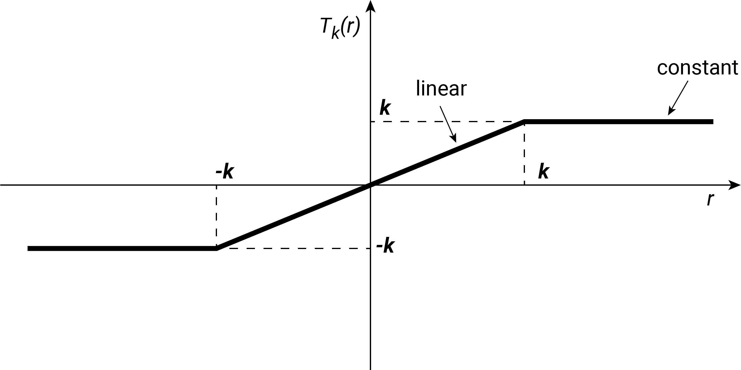
We begin by introducing the truncature operator. For given constant k>0k>0 we define the cut function Tk:ℝ→ℝT_{k}:\mathbb{R}\rightarrow\mathbb{R} as

Tk​(r)={−k,ifr≤−k,r,if|r|<k,k,ifr≥k,T_{k}\left(r\right)=\left\{\begin{array}[]{r@{~}c@{~}l}-k,\text{if}&r\leq-k,&\\ r,\text{if}&|r|<k,&\\ k,\text{if}&r\geq k,&\end{array}\right.
Refer to caption
Figure 1. Trunction function

and for r∈ℝ,r\in\mathbb{R}, let us define the functions : r→r+:=m​a​x​(r,0)r\rightarrow r^{+}:=max(r,0) and r→s​i​g​n0​(r)r\rightarrow sign_{0}(r) the usual sign function which is defined by

r→s​i​g​n0​(r):={−1,on]−∞,0[,1,on]0,∞[,0,ifr=0.r\rightarrow sign_{0}(r):=\left\{\begin{array}[]{r@{~}c@{~}l}-1,&\text{on}&]-\infty,0[,\\ 1,&\text{on}&]0,\infty[,\\ 0,&\text{if}&r=0.\end{array}\right.

and

r→s​i​g​n0+​(r):={1,ifr>0,0,ifr≤0.r\rightarrow sign_{0}^{+}(r):=\left\{\begin{array}[]{r@{~}c@{~}l}1,&\text{if}&r>0,\\ 0,&\text{if}&r\leq 0.\end{array}\right.

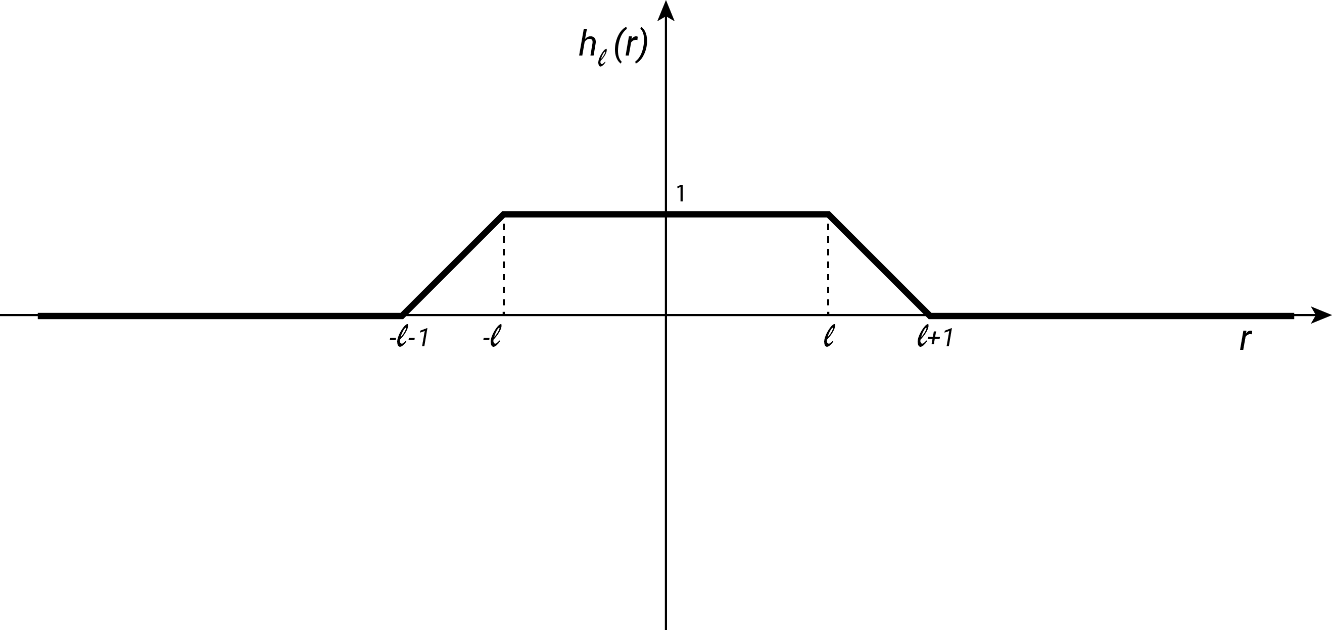
Let hl:ℝ→ℝh_{l}:\mathbb{R}\rightarrow\mathbb{R} be defined by hl​(r):=m​i​n​((l+1−|r|)+,1)h_{l}(r):=min((l+1-|r|)^{+},1) for each r∈ℝr\in\mathbb{R}.

Refer to caption
Figure 2. Function hl​(r)h_{l}(r)

For σ>0,\sigma>0, we define Hσ+:ℝ→ℝH_{\sigma}^{+}:\mathbb{R}\rightarrow\mathbb{R} by

Hσ+​(r):={0,ifr<0,1σ​r,if0≤r≤σ,1,ifr>σ.H_{\sigma}^{+}(r):=\left\{\begin{array}[]{l@{~}l}0,\text{if}&r<0,\\ \dfrac{1}{\sigma}r,\text{if}&0\leq r\leq\sigma,\\ 1,\text{if}&r>\sigma.\end{array}\right.

and Hσ:ℝ→ℝH_{\sigma}:\mathbb{R}\rightarrow\mathbb{R} by

Hσ​(r):={−1,ifr<−σ,1σ​r,if−σ≤r≤σ,1,ifr>σ.H_{\sigma}(r):=\left\{\begin{array}[]{l@{~}l}-1,\text{if}&r<-\sigma,\\ \dfrac{1}{\sigma}r,\text{if}&-\sigma\leq r\leq\sigma,\\ 1,\text{if}&r>\sigma.\end{array}\right.

3. Notion of solutions

3.1. Weak solutions

Definition 3.1.

A weak solution of (E,f)(E,f) is a pair of functions (u,b)∈W01,p→​(Ω)×L1​(Ω)(u,b)\in W_{0}^{1,{\overrightarrow{p}}}(\Omega)\times L^{1}(\Omega) satsfaying F⁡(u)∈(Ll​o​c1​(Ω))N,b∈β⁡(u)F(u)\in(L_{loc}^{1}(\Omega))^{N},b\in\beta(u) almost everywhere in Ω\Omega and

b−d​i​v​(a⁡(x,D​u)+F⁡(u))=f​i​n​D′​(Ω).b-div(a(x,Du)+F(u))=f\hskip 5.69054ptin\hskip 5.69054ptD^{\prime}(\Omega). (3.1)

3.2. Renormalized solutions

Definition 3.2.

A renormalized solution of (E,f)(E,f) is a pair of functions (u,b)(u,b) satisfying the following conditions:

(𝐑1)(\mathbf{R}_{1}) u:Ω→ℝu:\Omega\rightarrow\mathbb{R} is measurable, b∈L1​(Ω),u⁡(x)∈D⁡(β⁡(x))b\in L^{1}(\Omega),u(x)\in D(\beta(x)) and b⁡(x)∈β⁡(u⁡(x))b(x)\in\beta(u(x)) for a.e. x∈Ωx\in\Omega.

(𝐑2)(\mathbf{R}_{2}) For each k>0,Tk​(u)∈W01,p→​(Ω)k>0,T_{k}(u)\in W_{0}^{1,{\overrightarrow{p}}}(\Omega) and

∫Ωb.h⁡(u)​ϕ+∫Ω(a⁡(x,D⁡(u))+F⁡(u)).D⁡(h⁡(u)​ϕ)=∫Ωf​h​(u)​ϕ,\int_{\Omega}b.h(u)\phi+\int_{\Omega}(a(x,D(u))+F(u)).D(h(u)\phi)=\int_{\Omega}fh(u)\phi, (3.2)

holds for all h∈Cc1​(ℝ)h\in C_{c}^{1}(\mathbb{R}) and all ϕ∈W01,p→​(Ω)∩L∞​(Ω)\phi\in W_{0}^{1,{\overrightarrow{p}}}(\Omega)\cap L^{\infty}(\Omega).

(𝐑3)(\mathbf{R}_{3}) ∫{k<|u|<k+1}a(x,Du).Du⟶0\int_{\{k<|u|<k+1\}}a(x,Du).Du\longrightarrow 0 as k⟶∞k\longrightarrow\infty.

4. Main results

In this section, we will first state the existence and uniqueness of renormalized solutions for (E,f).(E,f). Then, we will prove that the renormalized solution of (E,f)(E,f) is a weak solution.

Theorem 4.1.

For f∈L1​(Ω)f\in L^{1}(\Omega), there exists at least one renormalized solution (u,b)(u,b) of (E,f)(E,f).

Theorem 4.2.

Let β:Ω×ℝ→2ℝ\beta:\Omega\times\mathbb{R}\rightarrow 2^{\mathbb{R}} be such that β(x,.)\beta(x,.) is strictly monotone for almost every x∈Ωx\in\Omega. For f∈L1​(Ω),f\in L^{1}(\Omega), let (u,b),(u~,b~)(u,b),(\widetilde{u},\widetilde{b}) be renormalized solutions of (E,f)(E,f). Then u=u~u=\widetilde{u} and b=b~.b=\widetilde{b}.

Proposition 4.3.

Let (u,b)(u,b) be a renormalized solution of (E,f)(E,f) for f∈L∞​(Ω)f\in L^{\infty}(\Omega). Then u∈W1,p→​(Ω)∪L∞​(Ω)u\in W^{1,{\overrightarrow{p}}}(\Omega)\cup L^{\infty}(\Omega) and thus, in particular, uu is a weak solution of (E,f)(E,f).

To prove Theorem 4.1, we will introduce and solve approximation problems. To this end, for f∈L1​(Ω)f\in L^{1}(\Omega) and m,n∈ℕm,n\in\mathbb{N} we define fm,n:Ω→ℝf_{m,n}:\Omega\rightarrow\mathbb{R} by

fm,n​(x)=m​a​x​(m​i​n​(f⁡(x),m),−n)f_{m,n}(x)=\displaystyle max(min(f(x),m),-n)

for almost every x∈Ωx\in\Omega. Clearly, fm,n∈L∞​(Ω)f_{m,n}\in L^{\infty}(\Omega) for each m,n∈ℕ,m,n\in\mathbb{N}, |fm,n​(x)|≤|f⁡(x)||f_{m,n}(x)|\leq|f(x)| a,e. in Ω\Omega, hence limn→∞limm→∞fm,n=f\displaystyle\lim_{n\rightarrow\infty}\lim_{m\rightarrow\infty}f_{m,n}=f in L1​(Ω)L^{1}(\Omega) and almost everywhere in Ω\Omega. The next theorem will give us existence of renormalized solutions (um,n,bm,n)(u_{m,n},b_{m,n}) of (E,fm,n)(E,f_{m,n}) for each m,n∈Ωm,n\in\Omega.

5. Case where f∈L∞​(Ω)f\in L^{\infty}(\Omega)

Theorem 5.1.

For f∈L∞​(Ω)f\in L^{\infty}(\Omega), there exists at least one renormalized solution (u,b)(u,b) of (E,f)(E,f).

The following section will be devoted to prove of Theorem 5.1, and we will divide it into several steps.

5.1. Approximate solution for L∞L^{\infty}- data

First we will introduce the approximate problem to (E,f)(E,f) for f∈L∞​(Ω)f\in L^{\infty}(\Omega) and for which the existence can be proved by standard variational arguments. For 0<ε≤1,0<\varepsilon\leq 1, let βε:ℝ⟼ℝ\beta_{\varepsilon}:\mathbb{R}\longmapsto\mathbb{R} be the Yosida approximation of β\beta (see [16]). We introduce the operators

A1,ε:W01,p→​(Ω)→W−1,p′→​(Ω),\mathit{A}_{1,\varepsilon}:W_{0}^{1,{\overrightarrow{p}}}(\Omega)\rightarrow W^{-1,{\overrightarrow{p^{\prime}}}}(\Omega),
u→βε​(T1/ε​(u))+ε​arctan⁡(u)−d​i​v​a​(x,D​u)u\rightarrow\beta_{\varepsilon}(T_{1/\varepsilon}(u))+\varepsilon\arctan(u)-diva(x,Du)

and

A2,ε:W01,p→​(Ω)→W−1,p′→​(Ω),\mathit{A}_{2,\varepsilon}:W_{0}^{1,{\overrightarrow{p}}}(\Omega)\rightarrow W^{-1,{\overrightarrow{p^{\prime}}}}(\Omega),
u→−d​i​v​F​(T1/ε​(u)).u\rightarrow-divF(T_{1/\varepsilon}(u)).

Because of (𝐇2)−(𝐇3)(\mathbf{H}_{2})-(\mathbf{H}_{3}) , A1/ε\mathit{A}_{1/\varepsilon} is well-defined and monotone (see [28] for instance).
Since βε∘T1/ε\beta_{\varepsilon}\circ T_{1/\varepsilon} is bounded and continuous and thanks to the growth condition (H2)(H_{2}) on aa, it follows that A1,ε\mathit{A}_{1,\varepsilon} is hermicontinuous (see [28]). From the continuity and boundedness of F∘T1/ε,F\circ T_{1/\varepsilon}, it follows that A2,ε\mathit{A}_{2,\varepsilon} is strongly continuous. Therefore the operator Aε:=A1,ε+A2,ε\mathit{A}_{\varepsilon}:=\mathit{A}_{1,\varepsilon}+\mathit{A}_{2,\varepsilon} is pseudomonotone. Using the monotonicity of βε\beta_{\varepsilon}, the Gauss-Green Theorem for Sobolev functions and the boundary condition on the convection term ∫ΩF⁡(T1/ε​(u)).D​u\int_{\Omega}F(T_{1/\varepsilon}(u)).Du, we show by using similar arguments as in [12] that Aε\mathit{A}_{\varepsilon} is coercive and bounded. Then it follows from [28] Theorem 2.72.7 that Aε\mathit{A}_{\varepsilon} is surjective, i.e., for each 0<ε≤10<\varepsilon\leq 1 and f∈W−1,p′→​(Ω)f\in W^{-1,{\overrightarrow{p^{\prime}}}}(\Omega) there exists a solution uε∈W01,p→​(Ω)u_{\varepsilon}\in W_{0}^{1,{\overrightarrow{p}}}(\Omega) of the problem

(Eε,f)​{βε​(T1/ε​(uε))+ε​arctan⁡(uε)−d​i​v​(a⁡(x,D​uε)+F⁡((T1/ε​(uε))))=fin ​Ω,uε=0on ​∂Ω,(E_{\varepsilon},f)\left\{\begin{array}[]{l@{~}l}\displaystyle\beta_{\varepsilon}(T_{1/\varepsilon}(u_{\varepsilon}))+\varepsilon\arctan(u_{\varepsilon})-div(a(x,Du_{\varepsilon})+F((T_{1/\varepsilon}(u_{\varepsilon}))))=f&\text{in }\Omega,\\ u_{\varepsilon}=0&\text{on }\partial\Omega,\end{array}\right.

such that the following inequality holds for all ϕ∈W01,p→​(Ω)\phi\in W_{0}^{1,{\overrightarrow{p}}}(\Omega)

∫Ω(βε​(T1/ε​(uε))+ε​arctan⁡(u))​ϕ+∫Ω(a⁡(x,D⁡(uε))+F⁡(T1/ε​(uε))).D​ϕ=<f,ϕ>\int_{\Omega}(\beta_{\varepsilon}(T_{1/\varepsilon}(u_{\varepsilon}))+\varepsilon\arctan(u))\phi+\int_{\Omega}(a(x,D(u_{\varepsilon}))+F(T_{1/\varepsilon}(u_{\varepsilon}))).D\phi=<f,\phi> (5.1)

where <.,.><.,.> denotes the duality pairing between W01,p→​(Ω)W_{0}^{1,{\overrightarrow{p}}}(\Omega) and W−1,p′→​(Ω).W^{-1,{\overrightarrow{p^{\prime}}}}(\Omega).

Proposition 5.2.

For 0<ε≤10<\varepsilon\leq 1 fixed and f,f~∈L∞​(Ω)f,\widetilde{f}\in L^{\infty}(\Omega), let uε,u~ε∈W01,p→​(Ω)u_{\varepsilon},\widetilde{u}_{\varepsilon}\in W_{0}^{1,{\overrightarrow{p}}}(\Omega) be solutions of (Eε,f)(E_{\varepsilon},f) and (Eε,f~)(E_{\varepsilon},\widetilde{f}), respectively, then, the follwing comparison principle holds:

ε​∫Ω(arctan⁡(uε)−arctan⁡(u~ε))+≤∫Ω(f−f~)​s​i​g​n0+​(uε−u~ε).\varepsilon\int_{\Omega}(\arctan(u_{\varepsilon})-\arctan(\widetilde{u}_{\varepsilon}))^{+}\leq\int_{\Omega}(f-\widetilde{f})sign_{0}^{+}(u_{\varepsilon}-\widetilde{u}_{\varepsilon}). (5.2)
Proof.

We use the test function φ=Hσ+​(uε−u~ε)\varphi=H_{\sigma}^{+}(u_{\varepsilon}-\widetilde{u}_{\varepsilon}) in the weak formulation (5.1)(\ref{eq5.1}) for uεu_{\varepsilon} and u~ε\widetilde{u}_{\varepsilon}. Substracting the resulting inequalties, we obtain

Il,δ1+Il,δ2+Il,δ3+Il,δ4=Il,δ5,I_{l,\delta}^{1}+I_{l,\delta}^{2}+I_{l,\delta}^{3}+I_{l,\delta}^{4}=I_{l,\delta}^{5},

where

Il,δ1=∫Ω(βε​T1ε​(uε)−βε​(T1ε​(u~ε)))​Hδ+​(uε−u~ε)I_{l,\delta}^{1}=\int_{\Omega}(\beta_{\varepsilon}T_{\frac{1}{\varepsilon}}(u_{\varepsilon})-\beta_{\varepsilon}(T_{\frac{1}{\varepsilon}}(\widetilde{u}_{\varepsilon})))H_{\delta}^{+}(u_{\varepsilon}-\widetilde{u}_{\varepsilon})
Il,δ2=∫Ω(ε​arctan⁡(uε)−ε​arctan⁡(u~ε))​Hδ+​(uε−u~ε),I_{l,\delta}^{2}=\int_{\Omega}(\varepsilon\arctan(u_{\varepsilon})-\varepsilon\arctan(\widetilde{u}_{\varepsilon}))H_{\delta}^{+}(u_{\varepsilon}-\widetilde{u}_{\varepsilon}),
Il,δ3=∫Ωa⁡(x,D​uε)−a⁡(x,D​u~ε).D​Hδ+​(uε−u~ε),I_{l,\delta}^{3}=\int_{\Omega}a(x,Du_{\varepsilon})-a(x,D\widetilde{u}_{\varepsilon}).DH_{\delta}^{+}(u_{\varepsilon}-\widetilde{u}_{\varepsilon}),
Il,δ4=∫Ω(F⁡(T1ε​(uε))−F⁡(T1ε​(u~ε))).D​Hδ+​(uε−u~ε)I_{l,\delta}^{4}=\int_{\Omega}(F(T_{\frac{1}{\varepsilon}}(u_{\varepsilon}))-F(T_{\frac{1}{\varepsilon}}(\widetilde{u}_{\varepsilon}))).DH_{\delta}^{+}(u_{\varepsilon}-\widetilde{u}_{\varepsilon})
Il,δ5=∫Ω(f−f~)​Hδ+​(uε−u~ε).I_{l,\delta}^{5}=\int_{\Omega}(f-\widetilde{f})H_{\delta}^{+}(u_{\varepsilon}-\widetilde{u}_{\varepsilon}).

Passing to the limit with σ→0\sigma\rightarrow 0, (5.2)(\ref{eq5.2}) follows. ∎

Remark 5.3.

Let f,f~∈L∞​(Ω)f,\widetilde{f}\in L^{\infty}(\Omega) be such that f≤f~f\leq\widetilde{f} almost everywhere in Ω,\Omega, ε>0\varepsilon>0 and uε,u_{\varepsilon}, u~ε∈W01,p→​(Ω)\widetilde{u}_{\varepsilon}\in W_{0}^{1,{\overrightarrow{p}}}(\Omega) be solutions of (Eε,f)(E_{\varepsilon},f) and (Eε,f~)(E_{\varepsilon},\widetilde{f}), respectively, then it is an immediate consequence of Propsition 5.2 is that uε≤u~εu_{\varepsilon}\leq\widetilde{u}_{\varepsilon} almost everywhere in Ω\Omega. Furthermore, from the monotonocity of βε∘T1/ε\beta_{\varepsilon}\circ T_{1/\varepsilon} it follows that also

βε​(T1/ε​(uε))≤βε​(T1/ε​(u~ε))\beta_{\varepsilon}(T_{1/\varepsilon}(u_{\varepsilon}))\leq\beta_{\varepsilon}(T_{1/\varepsilon}(\widetilde{u}_{\varepsilon}))

a,e. in Ω\Omega.

5.2. A priori estimates

Lemma 5.4.

For 0<ε≤10<\varepsilon\leq 1 and f∈L∞​(Ω)f\in L^{\infty}(\Omega) let 𝑂𝑃𝐸𝑁uε∈W01,p→​(Ω))u_{\varepsilon}\in W_{0}^{1,{\overrightarrow{p}}}(\Omega)) be a solution of (Eε,f)(E_{\varepsilon},f). Then
𝑂𝑃𝐸𝑁i)i) There exists a constant C1=C1​(‖f‖∞,λ,pi,N)>0,C_{1}=C_{1}\displaystyle(||f||_{\infty},\lambda,p_{i},N)>0, not depending on ε\varepsilon, such that

‖|uε|‖≤C1.|||u_{\varepsilon}|||\leq C_{1}. (5.3)

OPENi​i)ii) for all 0<ε≤1,0<\varepsilon\leq 1, we have

‖βε​(T1/ε​(uε))‖∞≤‖f‖∞||\beta_{\varepsilon}(T_{1/\varepsilon}(u_{\varepsilon}))||_{\infty}\leq||f||_{\infty} (5.4)

OPENi​i​i)iii) for all 0<ε≤10<\varepsilon\leq 1 and all l,k>0,l,k>0, we have

∫{l≤|u|≤k+l}a(x,Duε).Duε≤k∫{|uε|>l}|f|.\int_{\{l\leq|u|\leq k+l\}}a(x,Du_{\varepsilon}).Du_{\varepsilon}\leq k\int_{\{|u_{\varepsilon}|>l\}}|f|. (5.5)
Proof.

OPENi)i) Taking uεu_{\varepsilon} as a test function in (5.1)(\ref{eq5.1}) we obtain

∫Ω(βε​(T1/ε​(uε))+ε​arctan⁡(uε))​uε​𝑑x+∫Ωa⁡(x,D​uε).D​uε​𝑑x+∫ΩF⁡(T1/ε​(uε)).D​uε​𝑑x=∫Ωf​uε​𝑑x\int_{\Omega}(\beta_{\varepsilon}(T_{1/\varepsilon}(u_{\varepsilon}))+\varepsilon\arctan(u_{\varepsilon}))u_{\varepsilon}dx+\int_{\Omega}a(x,Du_{\varepsilon}).Du_{\varepsilon}dx+\int_{\Omega}F(T_{1/\varepsilon}(u_{\varepsilon})).Du_{\varepsilon}dx=\int_{\Omega}fu_{\varepsilon}dx

As the first term on the left-hand side is nonnegative and the integral over the convextion term vanishes by (H1)(H_{1}), we have

λ​∑i=1N∫Ω|∂uε∂xi|pi​𝑑x≤∑i=1N∫Ωai​(x,D​uε).∂uε∂xi​𝑑x≤∫Ωf​uε​𝑑x≤C​‖f‖∞​(∑i=1N∫Ω|∂uε∂xi|pi​𝑑x)1/pi.\displaystyle\lambda\sum_{i=1}^{N}\int_{\Omega}|\dfrac{\partial u_{\varepsilon}}{\partial x_{i}}|^{p_{i}}dx\leq\sum_{i=1}^{N}\int_{\Omega}a_{i}(x,Du_{\varepsilon}).\dfrac{\partial u_{\varepsilon}}{\partial x_{i}}dx\leq\int_{\Omega}fu_{\varepsilon}dx\leq C||f||_{\infty}(\sum_{i=1}^{N}\int_{\Omega}|\dfrac{\partial u_{\varepsilon}}{\partial x_{i}}|^{p_{i}}dx)^{1/p_{i}}.

due to the Hölder inequality. Thus ‖|uε|‖pi≤C2​‖|uε|‖|||u_{\varepsilon}|||^{p_{i}}\leq C_{2}|||u_{\varepsilon}|||, where C2C_{2} is a positive constant. Then we can deduce that uεu_{\varepsilon} remains bounded in W01,p→​(Ω)W_{0}^{1,{\overrightarrow{p}}}(\Omega) i.e.,

‖|uε|‖≤C1.|||u_{\varepsilon}|||\leq C_{1}.

OPENi​i)ii) Taking 1σ​[Tk+σ​(βε​(T1/ε​(uε)))−Tk​(βε​(T1/ε​(uε)))]\dfrac{1}{\sigma}[T_{k+\sigma}(\beta_{\varepsilon}(T_{1/\varepsilon}(u_{\varepsilon})))-T_{k}(\beta_{\varepsilon}(T_{1/\varepsilon}(u_{\varepsilon})))] as a test function in (5.1)(\ref{eq5.1}), passing to the limit with σ→0\sigma\rightarrow 0 and choosing k>‖f‖∞k>||f||_{\infty}, we obtain OPENi​i)ii).
OPENi​i​i)iii) For k,l>0k,l>0 fixed we take Tk​(uε−Tl​(uε))T_{k}(u_{\varepsilon}-T_{l}(u_{\varepsilon})) as a test function in (5.1)(\ref{eq5.1}).
Using ∫Ωa(x,Duε).DTk(uε−T(uε))dx=∫{l<|uε|<l+k}a(x,Duε).Duεdx\int_{\Omega}a(x,Du_{\varepsilon}).DT_{k}(u_{\varepsilon}-T(u_{\varepsilon}))dx=\int_{\{l<|u_{\varepsilon}|<l+k\}}a(x,Du_{\varepsilon}).Du_{\varepsilon}dx, and as the first term on the left-hand side is nonnegative and the convection term vanishes, we get

∫{l<|uε|<k+l}a(x,Duε).Duε≤∫ΩfTk(uε−Tl(uε))dx≤∫{|uε|>l}|f|dx.\int_{\{l<|u_{\varepsilon}|<k+l\}}a(x,Du_{\varepsilon}).Du_{\varepsilon}\leq\int_{\Omega}fT_{k}(u_{\varepsilon}-T_{l}(u_{\varepsilon}))dx\leq\int_{\{|u_{\varepsilon}|>l\}}|f|dx. (5.6)

∎

Remark 5.5.

For k>0k>0, from OPENi​i​i)iii) in Lemma 5.4, we deduce that

|{|uε|≥l}|≤C2l1−1p¯\displaystyle|\{|u_{\varepsilon}|\geq l\}|\leq\dfrac{C_{2}}{l^{1-\frac{1}{\overline{p}}}} (5.7)
∫{l≤|uε|≤k+l}a(x,Duε).Duε≤k||f||∞|{|uε|>l}|≤C2​(k)l1p¯−1\int_{\{l\leq|u_{\varepsilon}|\leq k+l\}}a(x,Du_{\varepsilon}).Du_{\varepsilon}\leq k||f||_{\infty}|\{|u_{\varepsilon}|>l\}|\leq\dfrac{C_{2}(k)}{l^{\frac{1}{\overline{p}}-1}} (5.8)

for any 0<ε≤10<\varepsilon\leq 1 and a constant C2​(k)>0C_{2}(k)>0 not depending on ε\varepsilon.

Indeed, let l>0l>0 large enough we have:

l|{|uε|≥l}|=∫{|uε|≥l}|Tl(uε)|dx≤C(∑i=1N∫Ω|∂Tl​(uε)∂xi|pi)1/pi≤C2l1/p¯l\lvert\{|u_{\varepsilon}|\geq l\}\rvert=\int_{\{|u_{\varepsilon}|\geq l\}}\lvert T_{l}(u_{\varepsilon})\rvert dx\leq C\Bigg(\sum_{i=1}^{N}\int_{\Omega}\Big\lvert\dfrac{\partial T_{l}(u_{\varepsilon})}{\partial x_{i}}\Big\rvert^{p_{i}}\Bigg)^{1/p_{i}}\leq C_{2}l^{1/\overline{p}}

with implies |{|uε|≥l}|≤C2l1/p¯−1\lvert\{|u_{\varepsilon}|\geq l\}\rvert\leq C_{2}l^{1/\overline{p}-1}. Then

liml→+∞|{|uε|≥l}|=0.\lim_{l\rightarrow+\infty}\lvert\{|u_{\varepsilon}|\geq l\}\rvert=0.

Therefore, (5.7) follows from (5.8).

5.3. Basic convergence results

Lemma 5.6.

For 0<ε≤10<\varepsilon\leq 1 and f∈L∞​(Ω)f\in L^{\infty}(\Omega), let uε∈W01,p→​(Ω)u_{\varepsilon}\in W_{0}^{1,{\overrightarrow{p}}}(\Omega) be a solution of (Eε,f)(E_{\varepsilon},f). There exist u∈W01,p→​(Ω),b∈L∞​(Ω)u\in W_{0}^{1,{\overrightarrow{p}}}(\Omega),b\in L^{\infty}(\Omega) such that for a not relabeled subsequence of (uε)0<ε≤1(u_{\varepsilon})_{0<\varepsilon\leq 1} as ε↦0:\varepsilon\mapsto 0:

uε⇀ui​n​W01,p→​(Ω)​a​n​d​a.e.i​n​Ω,u_{\varepsilon}\rightharpoonup u\hskip 28.45274ptin\hskip 5.69054ptW_{0}^{1,{\overrightarrow{p}}}(\Omega)\hskip 5.69054ptand\hskip 5.69054pta.e.\hskip 5.69054ptin\hskip 5.69054pt\Omega, (5.9)
Tk​(uε)⇀Tk​(u)i​n​W01,p→​(Ω)​a​n​d​s​t​r​o​n​g​l​y​i​n​Lq​(Ω),T_{k}(u_{\varepsilon})\rightharpoonup T_{k}(u)\hskip 14.22636ptin\hskip 5.69054ptW_{0}^{1,{\overrightarrow{p}}}(\Omega)\hskip 5.69054ptand\hskip 5.69054ptstrongly\hskip 5.69054ptin\hskip 5.69054ptL^{q}(\Omega), (5.10)
βε​(T1/ε​(uε))⇀bi​n​L∞​(Ω).\beta_{\varepsilon}(T_{1/\varepsilon}(u_{\varepsilon}))\rightharpoonup b\hskip 14.22636ptin\hskip 5.69054ptL^{\infty}(\Omega). (5.11)

Moreover, for any k>0k>0,

D​Tk​(uε)⇀D​Tk​(u)i​n​∏i=1NLpi​(Ω),DT_{k}(u_{\varepsilon})\rightharpoonup DT_{k}(u)\hskip 14.22636ptin\hskip 5.69054pt\prod_{i=1}^{N}L^{p_{i}}(\Omega), (5.12)
a(x,DTk(uε))⇀a(x,DTk(u))in∏i=1NLpi′(Ω).a(x,DT_{k}(u_{\varepsilon}))\rightharpoonup a(x,DT_{k}(u))\hskip 14.22636ptin\hskip 5.69054pt\prod_{i=1}^{N}L^{p_{i}^{{}^{\prime}}}(\Omega). (5.13)
Proof.

By combining Lemma 5.4 and Remark 5.5, we obtain (5.11)(\ref{eq5.11}). From (5.7),(5.3)(\ref{eq5.7}),(\ref{eq5.3}) and (2.5)(\ref{eq2.5}), we deduce with a classical argument (see [1]) that for a subsequence still indexed by ε\varepsilon, (5.9)−(5.10)(\ref{eq5.9})-(\ref{eq5.10}) and (5.12)(\ref{eq5.12}) hold as ε\varepsilon tends to 00, where uu is a mesurable function defined on Ω\Omega.

It is left to prove (5.13)(\ref{eq5.13}). For this, by (H2)(H_{2}) and (5.3)(\ref{eq5.3}) it follows that given any subsequence of (a​(x,D​Tk​(uε))ε)(a(x,DT_{k}(u_{\varepsilon}))_{\varepsilon}), there exists a subsequence, still denoted by (a​(x,D​Tk​(uε))ε)(a(x,DT_{k}(u_{\varepsilon}))_{\varepsilon}), such that a⁡(x,D​Tk​(uε))⇀Φka(x,DT_{k}(u_{\varepsilon}))\rightharpoonup\Phi_{k} in ∏i=1NLpi′(Ω)\displaystyle\prod_{i=1}^{N}L^{p_{i}^{{}^{\prime}}}(\Omega). We will prove that Φk=a⁡(x,D​Tk​(u))\Phi_{k}=a(x,DT_{k}(u)) a.e. on Ω\Omega. The proof consists of three steps.
Step 1: For every h∈W1,∞​(ℝ),h≤0h\in W^{1,\infty}(\mathbb{R}),h\leq 0 and s​u​p​p​(h)supp(h) compact, we will prove that

lim supε→0∫Ωa⁡(x,D​Tk​(uε)).D⁡[h⁡(uε)​(Tk​(uε)−Tk​(u))]​𝑑x≤0.\limsup_{\varepsilon\rightarrow 0}\int_{\Omega}a(x,DT_{k}(u_{\varepsilon})).D[h(u_{\varepsilon})(T_{k}(u_{\varepsilon})-T_{k}(u))]dx\leq 0. (5.14)

Taking h⁡(uε)​(Tk​(uε)−Tk​(u))h(u_{\varepsilon})(T_{k}(u_{\varepsilon})-T_{k}(u)) as a test function in (5.1)(\ref{eq5.1}), we have

∫Ω(βε(T1/ε(uε)+εarctan(uϵ))h(uε)(Tk(uε)−Tk(u))+∫Ωa(x,D(uε)).D[hε(Tk(uε)−Tk(u))]+∫ΩF(T1/ε(uε)).D[hε(Tk(uε)−Tk(u))]=∫Ωfh(uε)(Tk(uε)−Tk(u)).\begin{array}[]{c}\int_{\Omega}(\beta_{\varepsilon}(T_{1/\varepsilon}(u_{\varepsilon})+\varepsilon\arctan(u_{\epsilon}))h(u_{\varepsilon})(T_{k}(u_{\varepsilon})-T_{k}(u))+\int_{\Omega}a(x,D(u_{\varepsilon})).D[h_{\varepsilon}(T_{k}(u_{\varepsilon})-T_{k}(u))]\\ +\int_{\Omega}F(T_{1/\varepsilon}(u_{\varepsilon})).D[h_{\varepsilon}(T_{k}(u_{\varepsilon})-T_{k}(u))]=\int_{\Omega}fh(u_{\varepsilon})(T_{k}(u_{\varepsilon})-T_{k}(u)).\end{array} (5.15)

Using |hε​(Tk​(uε)−Tk​(u))|≤2​k​‖h‖∞|h_{\varepsilon}(T_{k}(u_{\varepsilon})-T_{k}(u))|\leq 2k||h||_{\infty}, by Lebesgue’s dominated convergence theorem we find that limε→0∫Ωf​h​(uε)​(Tk​(uε)−Tk​(u))=0\lim\limits_{\varepsilon\rightarrow 0}\int_{\Omega}fh(u_{\varepsilon})(T_{k}(u_{\varepsilon})-T_{k}(u))=0 and then
limε→0∫ΩF⁡(T1/ε​(uε)).D⁡[hε​(uε)​(Tk​(uε)−Tk​(u))]=0\lim\limits_{\varepsilon\rightarrow 0}\int_{\Omega}F(T_{1/\varepsilon}(u_{\varepsilon})).D[h_{\varepsilon}(u_{\varepsilon})(T_{k}(u_{\varepsilon})-T_{k}(u))]=0. By using the same arguments as in [4], we can prove that

lim supε→0∫Ωβε​(T1/ε​(uε)).[h⁡(uε)​(Tk​(uε)−Tk​(u))]​𝑑x≥0.\limsup_{\varepsilon\rightarrow 0}\int_{\Omega}\beta_{\varepsilon}(T_{1/\varepsilon}(u_{\varepsilon})).[h(u_{\varepsilon})(T_{k}(u_{\varepsilon})-T_{k}(u))]dx\geq 0.

Passing to the limit in (5.15)(\ref{eq5.15}) and using the above results, we obtain (5.14)(\ref{eq5.14}).

Step 2: We now prove that for every k>0k>0,

lim supε→0∫Ωa⁡(x,D​Tk​(uε)).[D⁡(Tk​(uε)−D​Tk​(u))]​𝑑x≤0.\limsup_{\varepsilon\rightarrow 0}\int_{\Omega}a(x,DT_{k}(u_{\varepsilon})).[D(T_{k}(u_{\varepsilon})-DT_{k}(u))]dx\leq 0. (5.16)

Indeed, for k>lk>l, take hl​(uε)​(Tk​(uε)−Tk​(u))h_{l}(u_{\varepsilon})(T_{k}(u_{\varepsilon})-T_{k}(u)) as a test function in (5.1)(\ref{eq5.1}). Letting ε→0\varepsilon\rightarrow 0 and then l→∞l\rightarrow\infty, we obtain

lim supε→0∫Ωa⁡(x,D​Tk​(uε)).D⁡[hl​(uε)​(Tk​(uε)−Tk​(u))]​𝑑x=E1+E2+E3.\limsup_{\varepsilon\rightarrow 0}\int_{\Omega}a(x,DT_{k}(u_{\varepsilon})).D[h_{l}(u_{\varepsilon})(T_{k}(u_{\varepsilon})-T_{k}(u))]dx=E_{1}+E_{2}+E_{3}.

where

E1=∫{|uε|≤k}hl(uε)a(x,DTk(uε)).[DTk(uε)−DTk(u)]dx,E2=∫{|uε|>k}hl(uε)a(x,DTk(uε)).(−DTk(u))]dx,E3=∫Ωhl′(uε)(Tk(uε)−Tk(u))a(x,DTk(uε)).Duεdx.\begin{array}[]{l}E_{1}=\int_{\{|u_{\varepsilon}|\leq k\}}h_{l}(u_{\varepsilon})a(x,DT_{k}(u_{\varepsilon})).[DT_{k}(u_{\varepsilon})-DT_{k}(u)]dx,\\ \\ E_{2}=\int_{\{|u_{\varepsilon}|>k\}}h_{l}(u_{\varepsilon})a(x,DT_{k}(u_{\varepsilon})).(-DT_{k}(u))]dx,\\ \\ E_{3}=\int_{\Omega}h_{l}^{{}^{\prime}}(u_{\varepsilon})(T_{k}(u_{\varepsilon})-T_{k}(u))a(x,DT_{k}(u_{\varepsilon})).Du_{\varepsilon}dx.\end{array}

Since l>kl>k, on the set {|uε|≤k}\{|u_{\varepsilon}|\leq k\} we have hl​(uε)=1h_{l}(u_{\varepsilon})=1 so that we can write

lim supε→0E1=lim supε→0∫Ωa⁡(x,D​Tk​(uε)).(D​Tk​(uε)−D​Tk​(u))​𝑑x.\limsup_{\varepsilon\rightarrow 0}E_{1}=\limsup_{\varepsilon\rightarrow 0}\int_{\Omega}a(x,DT_{k}(u_{\varepsilon})).(DT_{k}(u_{\varepsilon})-DT_{k}(u))dx.

For E2E_{2}, using Lebesgue’s dominated convergence theorem, we get

limε→0E2=∫{|uε|>k}hl(u)Φl+1.DTk(u)dx=0.\lim_{\varepsilon\rightarrow 0}E_{2}=\int_{\{|u_{\varepsilon}|>k\}}h_{l}(u)\Phi_{l+1}.DT_{k}(u)dx=0.

For E3E_{3}, we have

−∫Ωhl′(uε)(Tk(uε)−Tk(u))a(x,DTk(uε))Duεdx-\int_{\Omega}h_{l}^{{}^{\prime}}(u_{\varepsilon})(T_{k}(u_{\varepsilon})-T_{k}(u))a(x,DT_{k}(u_{\varepsilon}))Du_{\varepsilon}dx
≤2k∫{l<|uε|≤l+1}a(x,Duε)Duεdx.\leq 2k\int_{\{l<|u_{\varepsilon}|\leq l+1\}}a(x,Du_{\varepsilon})Du_{\varepsilon}dx.

Using (5.8)(\ref{eq5.8}), we deduce that

lim supl→∞lim supε→0(−∫Ωhl′(uε)(Tk(uε)−Tk(u))a(x,DTk(uε)).Duεdx)≤0.\limsup_{l\rightarrow\infty}\limsup_{\varepsilon\rightarrow 0}(-\int_{\Omega}h_{l}^{{}^{\prime}}(u_{\varepsilon})(T_{k}(u_{\varepsilon})-T_{k}(u))a(x,DT_{k}(u_{\varepsilon})).Du_{\varepsilon}dx)\leq 0.

Applying (5.14)(\ref{eq5.14}) with hh replaced by hl,l>kh_{l},l>k, we get

lim supε→0∫Ωa⁡(x,D​Tk​(uε)).[D​Tk​(uε)−D​Tk​(u)]​𝑑x\limsup_{\varepsilon\rightarrow 0}\int_{\Omega}a(x,DT_{k}(u_{\varepsilon})).[DT_{k}(u_{\varepsilon})-DT_{k}(u)]dx
≤lim supε→0(−∫Ωhl′(uε)(Tk(uε)−Tk(u))a(x,DTk(uε)).Duεdx).\hskip 113.81102pt\leq\limsup_{\varepsilon\rightarrow 0}(-\int_{\Omega}h_{l}^{{}^{\prime}}(u_{\varepsilon})(T_{k}(u_{\varepsilon})-T_{k}(u))a(x,DT_{k}(u_{\varepsilon})).Du_{\varepsilon}dx).

Now letting l→∞,l\rightarrow\infty, (5.16)(\ref{eq5.16}) yields.

Step 3: In this step, we prove by monotonicity arguments that for k>0k>0,
Φk=a⁡(x,D​Tk​(u))\Phi_{k}=a(x,DT_{k}(u)) for almost every x∈Ωx\in\Omega. Let ϕ∈D⁡(Ω)\phi\in D(\Omega) and α∈ℝ\alpha\in\mathbb{R}. Using (5.16)(\ref{eq5.16}), we have

α​limε→0∫Ωa⁡(x,D​Tk​(uε)).D​ϕ​𝑑x≥α​∫Ωa⁡(x,D⁡(Tk​(u)−α​ϕ)).D​ϕ​𝑑x.\alpha\lim_{\varepsilon\rightarrow 0}\int_{\Omega}a(x,DT_{k}(u_{\varepsilon})).D\phi dx\geq\alpha\int_{\Omega}a(x,D(T_{k}(u)-\alpha\phi)).D\phi dx.

Dividing by α>0\alpha>0 and α<0\alpha<0 and letting α→0\alpha\rightarrow 0, we obtain

limε→0∫Ωa⁡(x,D​Tk​(uε)).D​ϕ​𝑑x=∫Ωa⁡(x,D​Tk​(u)).D​ϕ​𝑑x.\lim_{\varepsilon\rightarrow 0}\int_{\Omega}a(x,DT_{k}(u_{\varepsilon})).D\phi dx=\int_{\Omega}a(x,DT_{k}(u)).D\phi dx. (5.17)

This means that for all k>0k>0, ∫ΩΦk.D​ϕ​𝑑x=∫Ωa⁡(x,D​Tk​(u)),\displaystyle\int_{\Omega}\Phi_{k}.D\phi dx=\int_{\Omega}a(x,DT_{k}(u)), and then
Φk=a⁡(x,D​Tk​(u))\Phi_{k}=a(x,DT_{k}(u)) in D′​(Ω)D^{\prime}(\Omega) for all k>0k>0. Hence Φk=a⁡(x,D​Tk​(u))\Phi_{k}=a(x,DT_{k}(u)) a.e. in Ω\Omega and then a⁡(x,D​Tk​(uε))⇀a⁡(x,D​Tk​(u))a(x,DT_{k}(u_{\varepsilon}))\rightharpoonup a(x,DT_{k}(u)) weakly in ∏i=1NLpi′(Ω).\displaystyle\prod_{i=1}^{N}L^{p_{i}^{{}^{\prime}}}(\Omega). ∎

Remark 5.7.

As an immediate consequence of (5.16)(\ref{eq5.16}) and (H3)(H_{3}) we obtain

limε→0∫Ωa(x,DTk(uε)−a(x,DTk(u)).(DTk(uε)−Tk(u))=0.\lim_{\varepsilon\rightarrow 0}\int_{\Omega}a(x,DT_{k}(u_{\varepsilon})-a(x,DT_{k}(u)).(DT_{k}(u_{\varepsilon})-T_{k}(u))=0. (5.18)

Let us see finally that

liml→∞∫l<|u|<l+1a⁡(x,D​T​(u)​𝑑x=0CLOSE.\lim_{l\rightarrow\infty}\int_{l<|u|<l+1}a(x,DT(u)dx=0. (5.19)

Endeed, for any l≥0l\geq 0 fixed we have

∫l<|u|<l+1a(x,D(uε).D(uε)dx=∫Ωa(x,DTl+1(uε).(DTl+1(uε)−DTl(uε))dx\int_{l<|u|<l+1}a(x,D(u_{\varepsilon}).D(u_{\varepsilon})dx=\int_{\Omega}a(x,DT_{l+1}(u_{\varepsilon}).(DT_{l+1}(u_{\varepsilon})-DT_{l}(u_{\varepsilon}))dx
=∫Ωa⁡(x,D​Tl+1​(uε)).D​Tl+1​(uε)​𝑑x−∫Ωa⁡(x,D​Tl​(uε)).D​Tl​(uε)​𝑑x.=\int_{\Omega}a(x,DT_{l+1}(u_{\varepsilon})).DT_{l+1}(u_{\varepsilon})dx-\int_{\Omega}a(x,DT_{l}(u_{\varepsilon})).DT_{l}(u_{\varepsilon})dx.

By (5.18)(\ref{eq5.18}) and passing to the limit as ε→0\varepsilon\rightarrow 0 for fixed l≥0l\geq 0 we obtain

limε→0∫{l<|uε|<l+1}a(x,D(uε)).D(uε)dx=∫Ωa(x,DTl+1(u)).DTl+1(u)dx−∫Ωa(x,DTl(u)).DTl(u)dx=∫{l<|u|<l+1}a(x,Du).D(u)dx.\begin{array}[]{cc}\lim_{\varepsilon\rightarrow 0}\int_{\{l<|u_{\varepsilon}|<l+1\}}a(x,D(u_{\varepsilon})).D(u_{\varepsilon})dx=\int_{\Omega}a(x,DT_{l+1}(u)).DT_{l+1}(u)dx&\\ -\int_{\Omega}a(x,DT_{l}(u)).DT_{l}(u)dx=\int_{\{l<|u|<l+1\}}a(x,Du).D(u)dx.\end{array} (5.20)

Therefore, taking l→+∞l\rightarrow+\infty in (5.20)(\ref{eq5.20}) and using the estimate (5.8)(\ref{eq5.8}) show that satisfies (R3)(R_{3}).

5.4. Proof of the existence result

We are now in position to conclude the proof of our main result presented in Theorem 5.1:

Proof.

Let h∈Cc1​(ℝ)h\in C_{c}^{1}(\mathbb{R}) and φ∈W01,p→​(Ω)∩L∞​(Ω)\varphi\in W_{0}^{1,{\overrightarrow{p}}}(\Omega)\cap L^{\infty}(\Omega). Taking hl​(uε)​h​(u)​(φ)h_{l}(u_{\varepsilon})h(u)(\varphi) as a test function in (5.1)(5.1), we obtain

Iε,l1+Iε,l2+Iε,l3+Iε,l4=Iε,l5I_{\varepsilon,l}^{1}+I_{\varepsilon,l}^{2}+I_{\varepsilon,l}^{3}+I_{\varepsilon,l}^{4}=I_{\varepsilon,l}^{5} (5.21)

where

Iε,l1=∫Ωβε​(T1/ε​(uε))​hl​(uε)​h​(u)​φ,I_{\varepsilon,l}^{1}=\int_{\Omega}\beta_{\varepsilon}(T_{1/\varepsilon}(u_{\varepsilon}))h_{l}(u_{\varepsilon})h(u)\varphi,
Iε,l2=ε​∫Ωarctan⁡(uε)​hl​(uε)​h​(u)​φ,I_{\varepsilon,l}^{2}=\varepsilon\int_{\Omega}\arctan(u_{\varepsilon})h_{l}(u_{\varepsilon})h(u)\varphi,
Iε,l3=∫Ωa⁡(x,D​uε).D⁡(hl​(uε)​h​(u)​φ),I_{\varepsilon,l}^{3}=\int_{\Omega}a(x,Du_{\varepsilon}).D(h_{l}(u_{\varepsilon})h(u)\varphi),
Iε,l4=∫ΩF⁡(T1/ε​(uε)).D⁡(hl​(uε)​h​(u)​φ),I_{\varepsilon,l}^{4}=\int_{\Omega}F(T_{1/\varepsilon}(u_{\varepsilon})).D(h_{l}(u_{\varepsilon})h(u)\varphi),
Iε,l5=∫Ωf​hl​(uε)​h​(u)​φ.I_{\varepsilon,l}^{5}=\int_{\Omega}fh_{l}(u_{\varepsilon})h(u)\varphi.

Step 1: Letting ε→0\varepsilon\rightarrow 0 obviously, we have

limε→0Iε,l2=0.\lim_{\varepsilon\rightarrow 0}I_{\varepsilon,l}^{2}=0. (5.22)

Using the convergence results (5.9),((5.11)CLOSE(\ref{eq5.9}),((\ref{eq5.11}) from Lemma 5.6 we can immediately calculate the following limits:

limε→0Iε,l1=∫Ωb​hl​(u)​h​(u)​φ,\lim_{\varepsilon\rightarrow 0}I_{\varepsilon,l}^{1}=\int_{\Omega}bh_{l}(u)h(u)\varphi, (5.23)
limε→0Iε,l5=∫Ωf​hl​(u)​h​(u)​φ.\lim_{\varepsilon\rightarrow 0}I_{\varepsilon,l}^{5}=\int_{\Omega}fh_{l}(u)h(u)\varphi. (5.24)

We write Iε,l3=Iε,l3,1+Iε,l3,2I_{\varepsilon,l}^{3}=I_{\varepsilon,l}^{3,1}+I_{\varepsilon,l}^{3,2} where

Iε,l3,1=∫Ωhl′(uε)a(x,Duε).Duεh(u)φ, Iε,l3,2=∫Ωhl(uε)a(x,Duε)D(h(u)φ)..\displaystyle I_{\varepsilon,l}^{3,1}=\int_{\Omega}h_{l}^{\prime}(u_{\varepsilon})a(x,Du_{\varepsilon}).Du_{\varepsilon}h(u)\varphi,\text{ }I_{\varepsilon,l}^{3,2}=\int_{\Omega}h_{l}(u_{\varepsilon})a(x,Du_{\varepsilon})D(h(u)\varphi)..

Using (5.8)(\ref{eq5.8}), we get the estimate

|limε→0Iε,l3,1|≤‖h‖∞​‖φ‖∞.C2​l−(1−1/p¯).|\lim_{\varepsilon\rightarrow 0}I_{\varepsilon,l}^{3,1}|\leq||h||_{\infty}||\varphi||_{\infty}.C_{2}l^{-(1-1/\bar{p})}. (5.25)

By Lebesgue’s dominated convergence theorem it follows that for any i∈{1,…,N}i\in\{1,...,N\}, we have

hl​(uε)​∂∂xi​(h⁡(u)​φ)→hl​(u)​∂∂xi​(h⁡(u)​φ)i​n​Lpi​a​s​ε→0.h_{l}(u_{\varepsilon})\dfrac{\partial}{\partial x_{i}}(h(u)\varphi)\rightarrow h_{l}(u)\dfrac{\partial}{\partial x_{i}}(h(u)\varphi)\hskip 14.22636ptin\hskip 5.69054ptL^{p_{i}}\hskip 5.69054ptas\hskip 5.69054pt\varepsilon\rightarrow 0.

Keeping in mind that Iε,l3,2=∫Ωhl​(uε)​a​(x,D​Tl+1​(uε)).D⁡(h⁡(u)​φ)I_{\varepsilon,l}^{3,2}=\int_{\Omega}h_{l}(u_{\varepsilon})a(x,DT_{l+1}(u_{\varepsilon})).D(h(u)\varphi) and by using (5.13)(\ref{eq5.13}), we get

limε→0Iε,l3,2=∫Ωhl​(u)​a​(x,D​Tl+1​(u)).D⁡(h⁡(u)​φ).\lim_{\varepsilon\rightarrow 0}I_{\varepsilon,l}^{3,2}=\int_{\Omega}h_{l}(u)a(x,DT_{l+1}(u)).D(h(u)\varphi). (5.26)

Let us write Iε,l4=Iε,l4,1+Iε,l4,2I_{\varepsilon,l}^{4}=I_{\varepsilon,l}^{4,1}+I_{\varepsilon,l}^{4,2}, where

Iε,l4,1=∫Ωhl′​(uε)​F​(T1/ε​(uε)).D​uε​h​(u)​φ,I_{\varepsilon,l}^{4,1}=\int_{\Omega}h_{l}^{\prime}(u_{\varepsilon})F(T_{1/\varepsilon}(u_{\varepsilon})).Du_{\varepsilon}h(u)\varphi,
Iε,l4,2=∫Ωhl​(uε)​F​(T1/ε​(uε)).D⁡(h⁡(u)​φ).I_{\varepsilon,l}^{4,2}=\int_{\Omega}h_{l}(u_{\varepsilon})F(T_{1/\varepsilon}(u_{\varepsilon})).D(h(u)\varphi).

For any l∈ℕl\in\mathbb{N}, there exists ε0​(l)\varepsilon_{0}(l) such that for all ε<ε0​(l),\varepsilon<\varepsilon_{0}(l),

Iε,l4,1=∫Ωhl′​(Tl+1​(uε))​F​(Tl+1​(uε)).h⁡(u)​φ.I_{\varepsilon,l}^{4,1}=\int_{\Omega}h_{l}^{\prime}(T_{l+1}(u_{\varepsilon}))F(T_{l+1}(u_{\varepsilon})).h(u)\varphi. (5.27)

Using the Gauss-Green Theorem for Sobolev functions in (5.27)(\ref{eq5.26}), we get for all ε<ε0​(l),\varepsilon<\varepsilon_{0}(l),

Iε,l4,1=−∫Ω∫0Tl+1​(uε)hl′(r)F(r)dr.D(h(u)φ).I_{\varepsilon,l}^{4,1}=-\int_{\Omega}\int_{0}^{T_{l+1}(u_{\varepsilon})}h_{l}^{\prime}(r)F(r)dr.D(h(u)\varphi). (5.28)

Now, using (5.9)(\ref{eq5.9}) and the Gauss-Green Theorem, after letting ε→0\varepsilon\rightarrow 0, we get

limε→Iε,l4,1=∫Ωhl′​(u)​F​(u).D​u​h​(u)​φ.\lim_{\varepsilon\rightarrow}I_{\varepsilon,l}^{4,1}=\int_{\Omega}h_{l}^{\prime}(u)F(u).Duh(u)\varphi. (5.29)

Choosing ε\varepsilon small enough, we can write

Iε,l4,2=∫Ωhl​(uε)​F​(Tl+1​(uε)).D⁡(h⁡(u)​φ),I_{\varepsilon,l}^{4,2}=\int_{\Omega}h_{l}(u_{\varepsilon})F(T_{l+1}(u_{\varepsilon})).D(h(u)\varphi), (5.30)

and conclude that

limε→0Iε,l4,2=∫Ωhl​(u)​F​(u).D⁡(h⁡(u)​φ).\lim\limits_{\varepsilon\rightarrow 0}I_{\varepsilon,l}^{4,2}=\int_{\Omega}h_{l}(u)F(u).D(h(u)\varphi). (5.31)

Step 2: Passage to the limit with l→∞l\rightarrow\infty.
Combining (5.21)(\ref{eq5.21}) and (5.22)−(5.31)(\ref{eq5.222})-(\ref{eq5.30}) we deduce that

Il1+Il2+Il3+Il4+Il5=Il6I_{l}^{1}+I_{l}^{2}+I_{l}^{3}+I_{l}^{4}+I_{l}^{5}=I_{l}^{6} (5.32)

where

Il1=∫Ωb​hl​(u)​h​(u)​φ,Il2=∫Ωhl​(u)​a​(x,D​Tl+1​(u)).D⁡(h⁡(u)​φ),|Il3|≤C2​|l−(1−1/p¯)|​|h||∞||φ||∞,Il4=∫Ωhl​(u)​F​(u).D⁡(h⁡(u)​φ),Il5=∫Ωhl′​(u)​F​(u).D​u​h​(u)​φ,Il6=∫Ωf​hl​(u)​h​(u)​φ.\begin{array}[]{lll}I_{l}^{1}=\int_{\Omega}bh_{l}(u)h(u)\varphi,&&I_{l}^{2}=\int_{\Omega}h_{l}(u)a(x,DT_{l+1}(u)).D(h(u)\varphi),\\ &&\\ |I_{l}^{3}|\leq C_{2}|l^{-(1-1/\bar{p})}||h||_{\infty}||\varphi||_{\infty},&&I_{l}^{4}=\int_{\Omega}h_{l}(u)F(u).D(h(u)\varphi),\\ &&\\ I_{l}^{5}=\int_{\Omega}h_{l}^{\prime}(u)F(u).Duh(u)\varphi,&&I_{l}^{6}=\int_{\Omega}fh_{l}(u)h(u)\varphi.\end{array}

Obviously, we have

limε→∞Il3=0.\lim_{\varepsilon\rightarrow\infty}I_{l}^{3}=0. (5.33)

Choosing m>0m>0 such that s​u​p​psupp h⊂[−m,m],h\subset[-m,m], we can replace uu by Tm​(u)T_{m}(u) in Il1,Il2,…,Il6,I_{l}^{1},I_{l}^{2},...,I_{l}^{6}, and

hl′(u)=hl′(Tm(u))=0ifl+1>m, hl(u)=hl(Tm(u))=0ifl>m.h_{l}^{\prime}(u)=h_{l}^{\prime}(T_{m}(u))=0\hskip 5.69054ptif\hskip 5.69054ptl+1>m,\text{ }h_{l}(u)=h_{l}(T_{m}(u))=0\hskip 5.69054ptif\hskip 5.69054ptl>m.

Therefore, letting l→∞l\rightarrow\infty and combining (5.32)(\ref{eq5.31}) with (5.33)(\ref{eq5.32}) we obtain

∫Ωb​h​(u)​φ+∫Ω(a⁡(x,D​u)+F⁡(u)).D⁡(h⁡(u)​φ)=∫Ωf​h​(u)​φ\int_{\Omega}bh(u)\varphi+\int_{\Omega}(a(x,Du)+F(u)).D(h(u)\varphi)=\int_{\Omega}fh(u)\varphi (5.34)

for all h∈Cc1​(ℝ)h\in C_{c}^{1}(\mathbb{R}) and all φ∈W01,p→​(Ω)∩L∞​(Ω)\varphi\in W_{0}^{1,{\overrightarrow{p}}}(\Omega)\cap L^{\infty}(\Omega).
Step 3: Subdifferential argument

It is left to prove that u⁡(x)∈D⁡(β⁡(x))u(x)\in D(\beta(x)) and b⁡(x)∈β⁡(u⁡(x))b(x)\in\beta(u(x)) for almost all x∈Ωx\in\Omega. Since β\beta is a maximal monotone graph, there exist a convex, l.s.c and proper function j:ℝ→[0,∞],j:\mathbb{R}\rightarrow[0,\infty], such that

β⁡(r)=∂j⁡(r)​for all ​r∈ℝ.\beta(r)=\partial j(r)\hskip 8.53581pt\text{for all\hskip 5.69054pt}r\in\mathbb{R}.

According to [16], for 0<ε≤1,jε:ℝ→ℝ0<\varepsilon\leq 1,j_{\varepsilon}:\mathbb{R}\rightarrow\mathbb{R} defined by jε​(r)=∫0rβε​(s)​𝑑sj_{\varepsilon}(r)=\int_{0}^{r}\beta_{\varepsilon}(s)ds has the following properties as in [33]

OPENi)i) For any 0<ε≤1,jε0<\varepsilon\leq 1,j_{\varepsilon} is convex and differentiable for all r∈ℝr\in\mathbb{R}, such that

jε′​(r)=βε​(r)​ for all ​r∈ℝ​ and any ​0<ε≤1.j_{\varepsilon}^{\prime}(r)=\beta_{\varepsilon}(r)\text{ for all }r\in\mathbb{R}\text{ and any }0<\varepsilon\leq 1.

OPENi​i)ii) jε​(r)→j​(r)j_{\varepsilon}(r)\rightarrow j(r) for all r∈ℝr\in\mathbb{R} as ε→0.\varepsilon\rightarrow 0.
From OPENi)i), it follows that for any 0<ε≤10<\varepsilon\leq 1

jε​(r)≥jε​(T1/ε​(uε))+(r−T1/ε​(uε))​βε​(T1/ε​(uε))j_{\varepsilon}(r)\geq j_{\varepsilon}(T_{1/\varepsilon}(u_{\varepsilon}))+(r-T_{1/\varepsilon}(u_{\varepsilon}))\beta_{\varepsilon}(T_{1/\varepsilon}(u_{\varepsilon})) (5.35)

holds for all r∈ℝr\in\mathbb{R} and almost everywhere in Ω\Omega.
Let E∪ΩE\cup\Omega be an arbitrary measurable set and χE\chi_{E} its characteristic function. We fix ε0>0.\varepsilon_{0}>0. Multiplying (5.35)(\ref{eq5.34}) by hl​(uε)​χEh_{l}(u_{\varepsilon})\chi_{E}, integrating over Ω\Omega and using OPENi​i)ii), we obtain

j⁡(r)​∫Ehl​(uε)≥∫Ejε0​(Tl+1​(uε))​hl​(uε)+(r−Tl+1​hl​(uε)​βε​(T1/ε​(uε))CLOSEj(r)\int_{E}h_{l}(u_{\varepsilon})\geq\int_{E}j_{\varepsilon_{0}}(T_{l+1}(u_{\varepsilon}))h_{l}(u_{\varepsilon})+(r-T_{l+1}h_{l}(u_{\varepsilon})\beta_{\varepsilon}(T_{1/\varepsilon}(u_{\varepsilon})) (5.36)

for all r∈ℝr\in\mathbb{R} and all 0<ε<m​i​n​(ε0,1l).0<\varepsilon<min(\varepsilon_{0},\dfrac{1}{l}).
As ε→0\varepsilon\rightarrow 0, taking into account that EE arbitrary we obtain from (5.36)(\ref{eq5.35})

j⁡(r)​hl​(u)≥jε0​(Tl+1​(u))​hl​(u)+b​hl​(u)​(r−Tl+1​(u))j(r)h_{l}(u)\geq j_{\varepsilon_{0}}(T_{l+1}(u))h_{l}(u)+bh_{l}(u)(r-T_{l+1}(u)) (5.37)

for all r∈ℝr\in\mathbb{R} and almost everywhere in Ω\Omega.
Passing to the limit with l→∞l\rightarrow\infty and then with ε0→0\varepsilon_{0}\rightarrow 0 in (5.37)(\ref{eq5.36}) finally yields

j⁡(r)≥j⁡(u⁡(x))+b⁡(x)​(r−u⁡(x))j(r)\geq j(u(x))+b(x)(r-u(x)) (5.38)

for all r∈ℝr\in\mathbb{R} and almost everywhere in Ω\Omega, hence u∈D⁡(β)u\in D(\beta) and b∈β⁡(u)b\in\beta(u) for almost everywhere in Ω\Omega. With this last step the proof of Theorem 5.1 is concluded. ∎

6. Case where f∈L1​(Ω)f\in L^{1}(\Omega)

6.1. Approximate solution for L1L^{1}- data

The comparison principle from proposition will be the tool in second approximation procedure. For f∈L1​(Ω)f\in L^{1}(\Omega) and m,n∈ℕm,n\in\mathbb{N} let fm,n∈L∞​(Ω)f_{m,n}\in L^{\infty}(\Omega) be defined as in Section 3. Using Propsition 4.3, we deduce that for any m,n∈ℕ,m,n\in\mathbb{N,} there exists um,n∈W01,p→​(Ω),bm,n∈L∞​(Ω)u_{m,n}\in W_{0}^{1,{\overrightarrow{p}}}(\Omega),b_{m,n}\in L^{\infty}(\Omega), such that (um,n,bm,n)(u_{m,n},b_{m,n}) is a renormalized solution of (E,fm,n)(E,f_{m,n}). Therefore

∫Ωbm,n​h​(um,n)​ϕ+∫Ω(a⁡(x,D​um,n)+F⁡(um,n)).D⁡(h⁡(um,n)​ϕ)=fm,n​h​(um,n)​ϕ\int_{\Omega}b_{m,n}h(u_{m,n})\phi+\int_{\Omega}(a(x,Du_{m,n})+F(u_{m,n})).D(h(u_{m,n})\phi)=f_{m,n}h(u_{m,n})\phi (6.1)

holds for all m,m, n∈ℕ,n\in\mathbb{N}, h∈Cc1​(ℝ),ϕ∈W01,p→​(Ω)∩L∞​(Ω)h\in C_{c}^{1}(\mathbb{R}),\phi\in W_{0}^{1,{\overrightarrow{p}}}(\Omega)\cap L^{\infty}(\Omega). In the next lemma, we give a priori estimates that will be important in the the following:

Lemma 6.1.

For m,n∈ℕ,m,n\in\mathbb{N,} let (um,n,bm,n)(u_{m,n},b_{m,n}) be a renormalized solution of (E,fm,n)(E,f_{m,n}) . Then,
𝑂𝑃𝐸𝑁i)i) For any k>0k>0 we have,

∑i=1N∫Ω|D​Tk​(um,n)|pi≤kγ​‖f‖1\sum_{i=1}^{N}\int_{\Omega}|DT_{k}(u_{m,n})|^{p_{i}}\leq\dfrac{k}{\gamma}\|f\|_{1} (6.2)

OPENi​i)ii) for any k>0k>0, there exists a constant C3​(k)>0C_{3}(k)>0, not depending on m,n∈ℕm,n\in\mathbb{N}, such that

∑i=1N∫Ω|D​Tk​(um,n)|pi≤C3​(k).\sum_{i=1}^{N}\int_{\Omega}|DT_{k}(u_{m,n})|^{p_{i}}\leq C_{3}(k). (6.3)

OPENi​i​i)iii) For m,n∈ℕm,n\in\mathbb{N}, we have:

‖bm,n‖1≤‖f‖1.\|b_{m,n}\|_{1}\leq\|f\|_{1}. (6.4)
Proof.

For l,k>0l,k>0, we plug hl​(um,n)​Tk​(um,n)h_{l}(u_{m,n})T_{k}(u_{m,n}) as a test function in (6.1)(\ref{eq6.1}). Then OPENi)i) and OPENi​i)ii) follows with similar arguments as used in the proof of Lemma 5.4. To prove OPENi​i​i)iii), we neglet the positve term

∫Ωa⁡(x,D​Tk​(um,n))​D​Tk​(um,n)\int_{\Omega}a(x,DT_{k}(u_{m,n}))DT_{k}(u_{m,n})

and keep

∫Ωbm,n​Tk​(um,n)≤∫Ωfm,n​T​(um,n).\int_{\Omega}b_{m,n}T_{k}(u_{m,n})\leq\int_{\Omega}f_{m,n}T(u_{m,n}). (6.5)

Since bm,n∈β⁡(um,n)b_{m,n}\in\beta(u_{m,n}) a.e. in Ω\Omega, it follows from (6.5)(\ref{eq6.4}) that

∫|um,n|>k|bm,n|≤∫Ω|f|.\int_{|u_{m,n}|>k}|b_{m,n}|\leq\int_{\Omega}|f|. (6.6)

and we find OPENi​i​i)iii) by passing to the limit with k→0k\rightarrow 0. ∎

By definition we have

fm,n≤fm+1,na​n​dfm,n+1≤fm,nf_{m,n}\leq f_{m+1,n}\hskip 11.38109ptand\hskip 11.38109ptf_{m,n+1}\leq f_{m,n} (6.7)

From Propostion 5.2 it follows that

um,nε≤um+1,nεa​n​dum,n+1ε≤um,nε,u_{m,n}^{\varepsilon}\leq u_{m+1,n}^{\varepsilon}\hskip 11.38109ptand\hskip 11.38109ptu_{m,n+1}^{\varepsilon}\leq u_{m,n}^{\varepsilon}, (6.8)

almost everywhere in Ω\Omega for any m,n∈ℕm,n\in\mathbb{N} and all ε>0\varepsilon>0.
Hence passing to the limit with ε→0\varepsilon\rightarrow 0 in (6.8)(\ref{eq6.7}) yields

um,n≤um+1,na​n​dum,n+1≤um,n,u_{m,n}\leq u_{m+1,n}\hskip 11.38109ptand\hskip 11.38109ptu_{m,n+1}\leq u_{m,n}, (6.9)

almost everywhere in Ω\Omega for any m,n∈ℕm,n\in\mathbb{N}.
Setting bε:=βε​(T1/ε​(uε)),b_{\varepsilon}:=\beta_{\varepsilon}(T_{1/\varepsilon}(u_{\varepsilon})), using (6.8)(\ref{eq6.7}), Remark 5.3 and the fact that bm,nε⇀bm,nb_{m,n}^{\varepsilon}\rightharpoonup b_{m,n} in L∞​(Ω)L^{\infty}(\Omega) and since this convergence preserves order we get

bm,n≤bm+1,na​n​dbm,n+1≤bm,nb_{m,n}\leq b_{m+1,n}\hskip 11.38109ptand\hskip 11.38109ptb_{m,n+1}\leq b_{m,n} (6.10)

almost everywhere in Ω\Omega for any m,n∈ℕm,n\in\mathbb{N}. By (6.10)(\ref{eq6.9}) and (6.4)(\ref{eq6.333}), for any n∈ℕn\in\mathbb{N} there exist bn∈L1​(Ω)b^{n}\in L^{1}(\Omega) such that bm,n→bnb_{m,n}\rightarrow b^{n} and m→∞m\rightarrow\infty in L1​(Ω)L^{1}(\Omega) and almost everywhere and b∈L1​(Ω)b\in L^{1}(\Omega), such that bn→bb^{n}\rightarrow b as n→∞n\rightarrow\infty in L1​(Ω)L^{1}(\Omega) and almost every where in Ω\Omega. By (6.9)(\ref{eq6.8}), the sequence (um,n)m(u_{m,n})_{m} is monotone increasing, hence, for any n∈ℕ,um,n→unn\in\mathbb{N},u_{m,n}\rightarrow u^{n} almost everywhere in Ω\Omega, where un:Ω→ℝ¯u^{n}:\Omega\rightarrow\mathbb{\overline{R}} is a mesurable function. In order to show that uu is finite almost everywhere we will give an estimate on the level sets of um,nu_{m,n} in the next lemma:

Lemma 6.2.

For m,n∈ℕm,n\in\mathbb{N} let (um,n,bm,n)(u_{m,n},b_{m,n}) be a renormalized solution of (E,fm,n)(E,f_{m,n}). Then, there exists a constant C4>0C_{4}>0, not depending on m,n∈ℕm,n\in\mathbb{N}, such that

|{|um,n|≥l}|≤C4l1p¯−1|\{|u_{m,n}|\geq l\}|\leq C_{4}l^{\frac{1}{\overline{p}}-1} (6.11)

for all l≥0l\geq 0.

Proof.

With the same arguments as in remark 5.5 we obtain

|{|um,n|}|≤C(p¯,N)lp¯−(∑i=1N∫Ω|DTk(um,n)|pi+|Ω|)|\{|u_{m,n}|\}|\leq C(\overline{p},N)l^{\overline{p}^{-}}(\sum_{i=1}^{N}\int_{\Omega}\left|DT_{k}(u_{m,n})\rvert^{p_{i}}+|\Omega|\right) (6.12)

for all m,n∈ℕm,n\in\mathbb{N} where C⁡(p¯,N)C(\overline{p},N) is the constant from Sobolev embedding in (2.5)(\ref{eq2.5}). Now we plug (6.2)(\ref{eq6.2}) into (6.12)(\ref{eq6.11}) to obtain (6.11)(\ref{eq6.10}). Note that, as (um,n)m(u_{m,n})_{m} is pointwise increasing with respect to mm,

limm→∞|{um,n≥l}|=|{un≥l}|\lim_{m\rightarrow\infty}|\{u_{m,n}\geq l\}|=|\{u^{n}\geq l\}| (6.13)

and

limm→∞|{um,n≤−l}|=|{un≤−l}|.\lim_{m\rightarrow\infty}|\{u_{m,n}\leq-l\}|=|\{u^{n}\leq-l\}|. (6.14)

Combining (6.11)(\ref{eq6.10}) with (6.13)(\ref{eq6.12}) and (6.14)(\ref{eq6.13}) we get

|{un≤−l}|+|{un>l}|≤C4l1p¯−1|\{u^{n}\leq-l\}|+|\{u^{n}>l\}|\leq C_{4}l^{\frac{1}{\overline{p}}-1} (6.15)

for any l≥1l\geq 1, hence unu^{n} is finite almost everywhere for n∈ℕn\in\mathbb{N}. By the same arguments we get

|{u<−l}|+|{u>l}|≤C4l1p¯−1|\{u<-l\}|+|\{u>l\}|\leq C_{4}l^{\frac{1}{\overline{p}}-1} (6.16)

from (6.15)(\ref{eq6.14}), hence uu is finite almost eveyrywhere. Now, since bm,n∈β⁡(um,n)b_{m,n}\in\beta(u_{m,n}) almost everywhere in Ω\Omega it follows by a subdifferential argument that bn∈β⁡(un)b^{n}\in\beta(u^{n}) and b∈β⁡(u)b\in\beta(u) a,e. in Ω\Omega.

∎

Remark 6.3.

If (um,n,bm,n)(u_{m,n},b_{m,n}) is renormalized solution of (E,fm,n)(E,f_{m,n}), using
hν​(um,n)​Tk​(um,n−Tl​(um,n))h_{\nu}(u_{m,n})T_{k}(u_{m,n}-T_{l}(u_{m,n})) as a test function in (6.1)(\ref{eq6.1}) , neglecting positive terms and passing to the limit with ν→∞\nu\rightarrow\infty we obtain

∫{l<|um,n|<l+k}a(x,Dum,n).Dum,n≤k⟮∫{|um,n|>l}∩{|f|<σ}|f|+∫{|f|>σ}|f|⟯\int_{\{l<|u_{m,n}|<l+k\}}a(x,Du_{m,n}).Du_{m,n}\leq k\Bigg\lgroup\int_{\{|u_{m,n}|>l\}\cap\{|f|<\sigma\}}|f|+\int_{\{|f|>\sigma\}}|f|\Bigg\rgroup (6.17)

for any k,σ>0,lk,\sigma>0,l. Now applying (6.11)(\ref{eq6.10}) to (6.17)(\ref{eq6.16}), we find that

∫{l<|um,n|<l+k}a(x,Dum,n).Dum,n≤σkC4l1p¯−1+k∫{|f|>σ}|f|\int_{\{l<|u_{m,n}|<l+k\}}a(x,Du_{m,n}).Du_{m,n}\leq\sigma kC_{4}l^{\frac{1}{\overline{p}}-1}+k\int_{\{|f|>\sigma\}}|f| (6.18)

holds for any k,σ>0,l≥0k,\sigma>0,l\geq 0 uniformly in m,n∈ℕ.m,n\in\mathbb{N}.

6.2. Basic convergence results

Lemma 6.4.

For m,n∈ℕm,n\in\mathbb{N} let (um,n,bm,n)(u_{m,n},b_{m,n}) be a renormalized soltuion of (E,Fm,n)(E,F_{m,n}). There exists a subsequence (m⁡(n))n(m(n))_{n} such that setting fn:=fm⁡(n),n,bn:=bm⁡(n),n,f_{n}:=f_{m(n),n},b_{n}:=b_{m(n),n}, un:=um⁡(n),nu_{n}:=u_{m(n),n} we have

un→ua​l​m​o​s​t​e​v​e​r​y​w​h​e​r​e​i​n​Ω.u_{n}\rightarrow u\hskip 11.38109ptalmost\hskip 5.69054pteverywhere\hskip 5.69054ptin\hskip 5.69054pt\Omega. (6.19)

Moreover, for any k>0,k>0,

Tk​(un)→Tk​(u)​i​n​W01,p→​(Ω),T_{k}(u_{n})\rightarrow T_{k}(u)\hskip 5.69054ptin\hskip 5.69054ptW_{0}^{1,{\overrightarrow{p}}}(\Omega), (6.20)
D​Tk​(un)⇀D​Tk​(u)​i​n​∏i=1NLpi​(Ω),DT_{k}(u_{n})\rightharpoonup DT_{k}(u)\hskip 5.69054ptin\hskip 5.69054pt\prod_{i=1}^{N}L^{p_{i}}(\Omega), (6.21)
a⁡(x,D​Tk​(un))⇀a⁡(x,D​Tk​(u))​i​n​∏i=1NLpi′​(Ω),a(x,DT_{k}(u_{n}))\rightharpoonup a(x,DT_{k}(u))\hskip 5.69054ptin\hskip 5.69054pt\prod_{i=1}^{N}L^{p_{i}^{\prime}}(\Omega), (6.22)

as n→∞n\rightarrow\infty.

Proof.

We construct a subsequence (m⁡(n))n(m(n))_{n}, such that

arctan⁡(um⁡(n),n)→arctan⁡(u),\arctan(u_{m(n),n})\rightarrow\arctan(u),
bn:=bm⁡(n),n→b,b_{n}:=b_{m(n),n}\rightarrow b,
fn:=fm⁡(n),n→ff_{n}:=f_{m(n),n}\rightarrow f

as n→∞n\rightarrow\infty in L1​(Ω)L^{1}(\Omega) and almost everywhere in Ω\Omega. It follows that (6.19)(\ref{eq6.18}) and (6.20)(\ref{eq6.19}) hold. Combining (6.20)(\ref{eq6.19}) with (6.3)(\ref{eq6.3}) we get Tk​(u)∈W01,p→​(Ω),Tk​(un)→Tk​(u)∈W01,p→​(Ω)T_{k}(u)\in W_{0}^{1,{\overrightarrow{p}}}(\Omega),T_{k}(u_{n})\rightarrow T_{k}(u)\in W_{0}^{1,{\overrightarrow{p}}}(\Omega) and (6.21)(\ref{eq6.20}) holds for any k>0k>0. From (6.2)(\ref{eq6.2}) and (H2),(H_{2}), it follows that for fixed k>0k>0, given any subsequence of (a⁡(x,D​Tk​(un)))n(a(x,DT_{k}(u_{n})))_{n} there exists a subsequence, still denoted by such that a​(x,D​Tk​(un))na(x,DT_{k}(u_{n}))_{n}, such that

a​(x,D​Tk​(un))n⇀Φk​i​n​∏i=1NLpi′​(Ω)a(x,DT_{k}(u_{n}))_{n}\rightharpoonup\Phi_{k}\hskip 8.53581ptin\hskip 5.69054pt\prod_{i=1}^{N}L^{p_{i}^{\prime}}(\Omega)

as n→∞n\rightarrow\infty. Since hl​(un)​(Tk​(un)−Tk​(u))h_{l}(u_{n})(T_{k}(u_{n})-T_{k}(u)) is an admissible test function in (6.1)(\ref{eq6.1}),

limn→∞sup∫Ωa⁡(x,D​Tk​(un))​D​(Tk​(un)−Tk​(u))≤0.\lim_{n\rightarrow\infty}\sup\int_{\Omega}a(x,DT_{k}(u_{n}))D(T_{k}(u_{n})-T_{k}(u))\leq 0. (6.23)

Then, (6.22)(\ref{eq6.21}) follows with the same arguments as int the proof of Lemma 5.6. ∎

Remark 6.5.

With the same arguments as in Remark 5.7, we have

limn→∞∫Ωa⁡(x,D​Tk​(un)−a⁡(x,D​Tk​(u))).D⁡(Tk​(un)−Tk​(u))=0,\lim_{n\rightarrow\infty}\int_{\Omega}a(x,DT_{k}(u_{n})-a(x,DT_{k}(u))).D(T_{k}(u_{n})-T_{k}(u))=0, (6.24)
liml→∞∫{l<|u|<l+1}a(x,Du).Du=0.\lim_{l\rightarrow\infty}\int_{\{l<|u|<l+1\}}a(x,Du).Du=0. (6.25)

6.3. Conclusion of the proof of Theorem 4.1

It is left to prove thet (u,b)(u,b) satisfies

∫Ωb​h​(u)​ϕ+∫Ω(a⁡(x,D​u)+F⁡(u)).D⁡(h⁡(u)​ϕ)=∫Ωf​h​(u)​ϕ.\int_{\Omega}bh(u)\phi+\int_{\Omega}(a(x,Du)+F(u)).D(h(u)\phi)=\int_{\Omega}fh(u)\phi. (6.26)

for all h∈Cc1​(ℝ)h\in C^{1}_{c}(\mathbb{R}) and ϕ∈W01,p→​(Ω)∩L∞​(Ω)\phi\in W^{1,{\overrightarrow{p}}}_{0}(\Omega)\cap L^{\infty}(\Omega). To this end, we take h∈Cc1​(ℝ)h\in C^{1}_{c}(\mathbb{R}) and ϕ∈W01,p→​(Ω)∩L∞​(Ω)\phi\in W^{1,{\overrightarrow{p}}}_{0}(\Omega)\cap L^{\infty}(\Omega) arbitrary and plug hl​(un)​h​(u)​ϕh_{l}(u_{n})h(u)\phi into (6.1)(\ref{eq6.1}) to obtain

In,l1+In,l2+In,l3=In,l4,I_{n,l}^{1}+I_{n,l}^{2}+I_{n,l}^{3}=I_{n,l}^{4}, (6.27)

where

In,l1=∫Ωbn​hl​(un)​h​(u)​ϕ,I_{n,l}^{1}=\int_{\Omega}b_{n}h_{l}(u_{n})h(u)\phi,
In,l2=∫Ωa⁡(x,D​un).D⁡(hl​(un)​h​(u)​ϕ),I^{2}_{n,l}=\int_{\Omega}a(x,Du_{n}).D(h_{l}(u_{n})h(u)\phi),
In,l3=∫ΩF⁡(un).D⁡(hl​(un)​h​(u)​ϕ),I^{3}_{n,l}=\int_{\Omega}F(u_{n}).D(h_{l}(u_{n})h(u)\phi),
Iε,l4=∫Ωfn​hl​(un)​h​(u)​ϕ.I^{4}_{\varepsilon,l}=\int_{\Omega}f_{n}h_{l}(u_{n})h(u)\phi.

Step 1. Passing to the limit as n→∞n\rightarrow\infty, applying the convergence results from Lemma 6.4 we get

limn→∞In,l1=∫Ωb​hl​(u)​h​(u)​ϕ,limn→∞In,l4=∫Ωf​hl​(u)​h​(u)​ϕ.\lim_{n\rightarrow\infty}I_{n,l}^{1}=\int_{\Omega}bh_{l}(u)h(u)\phi,\quad\lim_{n\rightarrow\infty}I_{n,l}^{4}=\int_{\Omega}fh_{l}(u)h(u)\phi. (6.28)

Let us write

In,l2=In,l2,1+In,l2,2,I_{n,l}^{2}=I_{n,l}^{2,1}+I_{n,l}^{2,2}, (6.29)

where

In,l2,1=∫Ωhl​(un)​a​(x,D​un).D⁡(h⁡(u)​ϕ),In,l2,2=∫Ωhl′​(un)​a​(x,D​un).D​un​h​(u)​ϕ.I_{n,l}^{2,1}=\int_{\Omega}h_{l}(u_{n})a(x,Du_{n}).D(h(u)\phi),\quad I_{n,l}^{2,2}=\int_{\Omega}h_{l}^{\prime}(u_{n})a(x,Du_{n}).Du_{n}h(u)\phi. (6.30)

With similar arguments as in the proof of (5.26)(\ref{eq5.25}) it follows that

limn→∞In,l2,1=∫Ωhl​(u)​a​(x,D​u).D⁡(h⁡(u)​ϕ).\lim_{n\rightarrow\infty}I_{n,l}^{2,1}=\int_{\Omega}h_{l}(u)a(x,Du).D(h(u)\phi). (6.31)

By (6.18)(\ref{eq6.17}), we get the estimate

|limn→∞In,l2,2|≤∥h∥∞∥ϕ∥∞(δC4l1p¯−1+∫{|f|>δ}|f|),|\lim_{n\rightarrow\infty}I_{n,l}^{2,2}|\leq\|h\|_{\infty}\|\phi\|_{\infty}\big(\delta C_{4}l^{\frac{1}{\overline{p}}-1}+\int_{\{|f|>\delta\}}|f|\big), (6.32)

for all n​∫ℕn\int\mathbb{N} and all l≥1l\geq 1, δ>0\delta>0. Next, we write

In,l3=In,l3,1+In,l3,2,I_{n,l}^{3}=I_{n,l}^{3,1}+I_{n,l}^{3,2},

where

limn→∞In,l3,1=∫Ωhl​(u)​F​(u).D⁡(h⁡(u)​ϕ),limn→∞In,l3,2=∫Ωhl′​(u)​F​(u).D​u​h​(u)​ϕ,\lim_{n\rightarrow\infty}I_{n,l}^{3,1}=\int_{\Omega}h_{l}(u)F(u).D(h(u)\phi),\lim_{n\rightarrow\infty}I_{n,l}^{3,2}=\int_{\Omega}h_{l}^{\prime}(u)F(u).Duh(u)\phi, (6.33)

follows with the same arguments as in (5.27)−(5.31)(\ref{eq5.26})-(\ref{eq5.30}).
Step 2. Passing to the limit as l→∞l\rightarrow\infty. Combining (6.27) with (6.28)-(6.33) we get for all δ>0\delta>0 and all l≥1l\geq 1

Il1+Il2+Il3+Il4+Il5=Il6,I_{l}^{1}+I_{l}^{2}+I_{l}^{3}+I_{l}^{4}+I_{l}^{5}=I_{l}^{6}, (6.34)

where

Il1=∫Ωb​hl​(u)​h​(u)​ϕ,Il2=∫Ωhl​(u)​a​(x,D​Tl+1​(u)).D⁡(h⁡(u)​ϕ)I_{l}^{1}=\int_{\Omega}bh_{l}(u)h(u)\phi,\quad I_{l}^{2}=\int_{\Omega}h_{l}(u)a(x,DT_{l+1}(u)).D(h(u)\phi)
|Il3|≤∥h∥∞∥ϕ∥∞(δC4l1p¯−1+∫{|f|>δ}|f|),|I_{l}^{3}|\leq\|h\|_{\infty}\|\phi\|_{\infty}\big(\delta C_{4}l^{\frac{1}{\overline{p}}-1}+\int_{\{|f|>\delta\}}|f|\big),

for any δ>0\delta>0 and

Il4=∫Ωhl′(u)F(u)h(u)ϕDu, Il5=∫Ωhl(u)F(u).D(h(u)ϕ), |Il6|=∫Ωfhl(u)h(u)ϕ.I_{l}^{4}=\int_{\Omega}h_{l}^{\prime}(u)F(u)h(u)\phi Du,\text{ }I_{l}^{5}=\int_{\Omega}h_{l}(u)F(u).D(h(u)\phi),\text{ }|I_{l}^{6}|=\int_{\Omega}fh_{l}(u)h(u)\phi.

Choosing m>0m>0 such that s​u​p​p​h⊂[−m,m]supph\subset[-m,m], we can replace uu by Tm​(u)T_{m}(u) in Il1,Il2,…,Il6I_{l}^{1},I_{l}^{2},\dots,I_{l}^{6} hence

liml→∞Il1=∫Ωb​h​(u)​ϕ,liml→∞Il2=∫Ωa⁡(x,D​u).D⁡(h⁡(u)​ϕ),\lim_{l\rightarrow\infty}I_{l}^{1}=\int_{\Omega}bh(u)\phi,\lim_{l\rightarrow\infty}I_{l}^{2}=\int_{\Omega}a(x,Du).D(h(u)\phi), (6.35)
liml→∞|Il3|≤∥h∥∞∥ϕ∥∞∫{|f|>σ}|f|,liml→∞Il4=0,\lim_{l\rightarrow\infty}|I_{l}^{3}|\leq\|h\|_{\infty}\|\phi\|_{\infty}\int_{\{|f|>\sigma\}}|f|,\lim_{l\rightarrow\infty}I_{l}^{4}=0, (6.36)
liml→∞|Il5|=∫ΩF⁡(u).D⁡(h⁡(u)​ϕ),liml→∞|Il6|=∫Ωf​h​(u)​ϕ,\lim_{l\rightarrow\infty}|I_{l}^{5}|=\int_{\Omega}F(u).D(h(u)\phi),\lim_{l\rightarrow\infty}|I_{l}^{6}|=\int_{\Omega}fh(u)\phi, (6.37)

for all δ>0\delta>0. Combining (6.34) with (6.35)-(6.37) we finally deduce that (6.1) holds for all h∈CC1​(ℝ)h\in C_{C}^{1}(\mathbb{R}) and all ϕ∈W01,p→​(Ω)∩L∞​(Ω)\phi\in W_{0}^{1,{\overrightarrow{p}}}(\Omega)\cap L^{\infty}(\Omega).
Hence (u,b)(u,b) satisfies (R1), (R2) and (R3) and the proof of the theorem is completed.

6.4. Proof of Theorem 4.2 (Uniqueness)

Lemma 6.6.

For f,f~∈L1​(Ω)f,\widetilde{f}\in L^{1}(\Omega) let (u,b)(u,b), (u~,b~)(\widetilde{u},\widetilde{b}) be the renormalized solutions to (E,f)(E,f) and (E,f~)(E,\widetilde{f}) respectively, then

∫Ω(b−b~)​S​i​g​n0+​(u−u~)​𝑑x≤∫Ω(f−f~)​S​i​g​n0+​(u−u~)​𝑑x,\int_{\Omega}(b-\widetilde{b})Sign_{0}^{+}(u-\widetilde{u})dx\leq\int_{\Omega}(f-\widetilde{f})Sign_{0}^{+}(u-\widetilde{u})dx, (6.38)

Proof. For δ>0\delta>0 let Hδ+H_{\delta}^{+} be a Lipschitz approximation of the s​i​g​n0+sign_{0}^{+} function. Since (u,b)(u,b), (u~,b~)(\widetilde{u},\widetilde{b}) are renormalized solutions, it follows that

Tl+1​(u),Tl+1​(u~)∈W01,p→​(Ω)∩L∞​(Ω)T_{l+1}(u),T_{l+1}(\widetilde{u})\in W_{0}^{1,{\overrightarrow{p}}}(\Omega)\cap L^{\infty}(\Omega) for all l>0l>0.

Hence Hδ+​(Tl+1​(u)−Tl+1​(u~))∈W01,p→​(Ω)∩L∞​(Ω)H_{\delta}^{+}(T_{l+1}(u)-T_{l+1}(\widetilde{u}))\in W_{0}^{1,{\overrightarrow{p}}}(\Omega)\cap L^{\infty}(\Omega) for l,δ>0l,\delta>0.
Now, we choose Hδ+​(Tl+1​(u)−Tl+1​(u~))H_{\delta}^{+}(T_{l+1}(u)-T_{l+1}(\widetilde{u})) as a test function in the renormalized formulation with h=hlh=h_{l} for (u,b)(u,b) and for (u~,b~)(\widetilde{u},\widetilde{b}) respectively. Subtracting the resulting equalities, we obtain

Il,δ1+Il,δ2+Il,δ3+Il,δ4+Il,δ5=Il,δ6,I_{l,\delta}^{1}+I_{l,\delta}^{2}+I_{l,\delta}^{3}+I_{l,\delta}^{4}+I_{l,\delta}^{5}=I_{l,\delta}^{6}, (6.39)

where K={0<Tl+1(u)−Tl+1<δ}K=\{0<T_{l+1}(u)-T_{l+1}<\delta\} and

Il,δ1=∫Ω(b​hl​(u)−b~​hl​(u~))​Hδ+​(Tl+1​(u)−Tl+1​(u~))​𝑑x,I_{l,\delta}^{1}=\int_{\Omega}(bh_{l}(u)-\widetilde{b}h_{l}(\widetilde{u}))H_{\delta}^{+}(T_{l+1}(u)-T_{l+1}(\widetilde{u}))dx,
Il,δ2=∫Ω(hl′(u)a(x,Du).Du−hl′(u~)a(x,Du~).Du~).Hδ+(Tl+1(u)−Tl+1(u~))dx,I_{l,\delta}^{2}=\int_{\Omega}(h_{l}^{\prime}(u)a(x,Du).Du-h_{l}^{\prime}(\widetilde{u})a(x,D\widetilde{u}).D\widetilde{u}).H_{\delta}^{+}(T_{l+1}(u)-T_{l+1}(\widetilde{u}))dx,
Il,δ3=1δ​∫K(hl​(u)​a​(x,D​u)−hl​(u~)​a​(x,D​u~)).D⁡(Tl+1​(u)−Tl+1​(u~))​𝑑x,I_{l,\delta}^{3}=\frac{1}{\delta}\int_{K}(h_{l}(u)a(x,Du)-h_{l}(\widetilde{u})a(x,D\widetilde{u})).D(T_{l+1}(u)-T_{l+1}(\widetilde{u}))dx,
Il,δ4=∫Ω(hl′(u)F(u).Du−hl′(u~)F(u~).Du~)Hδ+(Tl+1(u)−Tl+1(u~))dx,I_{l,\delta}^{4}=\int_{\Omega}(h_{l}^{\prime}(u)F(u).Du-h_{l}^{\prime}(\widetilde{u})F(\widetilde{u}).D\widetilde{u})H_{\delta}^{+}(T_{l+1}(u)-T_{l+1}(\widetilde{u}))dx,
Il,δ5=1δ​∫K(hl​(u)​F​(u)−hl​(u~)​F​(u~)).D⁡(Tl+1​(u)−Tl+1​(u~))​𝑑x,I_{l,\delta}^{5}=\frac{1}{\delta}\int_{K}(h_{l}(u)F(u)-h_{l}(\widetilde{u})F(\widetilde{u})).D(T_{l+1}(u)-T_{l+1}(\widetilde{u}))dx,
Il,δ6=∫Ω(f​hl​(u)−f~​hl​(u~))​Hδ+​(Tl+1​(u)−Tl+1​(u~))​𝑑x.I_{l,\delta}^{6}=\int_{\Omega}(fh_{l}(u)-\widetilde{f}h_{l}(\widetilde{u}))H_{\delta}^{+}(T_{l+1}(u)-T_{l+1}(\widetilde{u}))dx.

Using the same arguments as in [33] i.e., neglecting the nonnegative part of Il,δ3I_{l,\delta}^{3} and using that FF is locally Lipschitz continuous, we can pass to the limit as δ→0\delta\rightarrow 0.
Using the energy dissipation condition (R3)(R_{3}) we can pass the limit as l→∞l\rightarrow\infty and obtain (6.38).

Now we are in position to give the proof of Theorem 4.2:
Assuming f=f~f=\widetilde{f}, from lemma 6.66.6 we get

∫Ω(b−b~)​s​i​g​n0+​(u−u~)​𝑑x≤0,\int_{\Omega}(b-\widetilde{b})sign_{0}^{+}(u-\widetilde{u})dx\leq 0, (6.40)

hence (b−b~)​s​i​g​n0+​(u−u~)=0(b-\widetilde{b})sign_{0}^{+}(u-\widetilde{u})=0 almost everywhere in Ω\Omega. Now, let us write
Ω=Ω1∪Ω2\Omega=\Omega_{1}\cup\Omega_{2}, where Ω1:={x∈Ω:s​i​g​n0+​(u⁡(x)−u~​(x))=0},Ω2:={x∈Ω:(b⁡(x)−b~​(x))=0}\Omega_{1}:=\{x\in\Omega:sign_{0}^{+}(u(x)-\widetilde{u}(x))=0\},\Omega_{2}:=\{x\in\Omega:(b(x)-\widetilde{b}(x))=0\}. Since r↦β⁡(x,r)r\mapsto\beta(x,r) is strictly increasing for a,e. x∈Ωx\in\Omega, we can define the function β−1:ℝ→→ℝ\beta^{-1}:\mathbb{R}\rightarrow\rightarrow\mathbb{R} such that β−1=s\beta^{-1}=s for all (r,s)∈ℝ2(r,s)\in\mathbb{R}^{2} such that r∈β⁡(x,r)r\in\beta(x,r) for a,e. x∈Ωx\in\Omega. For a,e. x∈Ω2x\in\Omega_{2} we have b​(x)=b~​(x)b(x)=\widetilde{b}(x), hence u⁡(x)=β−1​(b⁡(x))=β−1​(b~​(x))=u~​(x)u(x)=\beta^{-1}(b(x))=\beta^{-1}(\widetilde{b}(x))=\widetilde{u}(x). Therefore, u​(x)=u~​(x)u(x)=\widetilde{u}(x) a,e. in Ω2\Omega_{2} and s​i​g​n0+​(u−u~)=0sign_{0}^{+}(u-\widetilde{u})=0. Interchanging the roles of uu and u~\widetilde{u} and respeating the arguments, we get s​i​g​n0+​(u~−u)=0sign_{0}^{+}(\widetilde{u}-u)=0 a,e. in Ω\Omega and we finally arrive at u=u~u=\widetilde{u} a,e. in Ω\Omega. Now, we write the renormalized formulation for (u,b)(u,b) and (u~,b~)(\widetilde{u},\widetilde{b}) respectively. Substracting the resulting equalities, we obtain

∫Ω(b−b~)​h​(u)​φ​𝑑x=0\int_{\Omega}(b-\widetilde{b})h(u)\varphi dx=0

for all h∈Cc1​(ℝ)h\in C_{c}^{1}(\mathbb{R}) and all φ∈Cc∞​(Ω)\varphi\in C_{c}^{\infty}(\Omega). Choosing h​(u)=hl​(u)h(u)=h_{l}(u) and passing to the limit with l→∞l\rightarrow\infty we find b=b~b=\widetilde{b} a,e. in Ω\Omega.

7. Proof of Proposition 4.3

Note that for ε,k>0\varepsilon,k>0, hl​(u)​1ε​Tε​(u−Tk​(u))h_{l}(u)\dfrac{1}{\varepsilon}T_{\varepsilon}(u-T_{k}(u)) as a test function in (3.2)(\ref{eq3.2}). Neglecting positive terms and passing to the limit with l→∞l\rightarrow\infty, we obtain

1ε∑i=1N∫k<|u|<k+ε|Du|pi≤∥f∥N(ϕ(k))(N−1)/N,\dfrac{1}{\varepsilon}\sum_{i=1}^{N}\int_{k<|u|<k+\varepsilon}|Du|^{p_{i}}\leq\lVert f\lVert_{N}(\phi(k))^{(N-1)/N}, (7.1)

where ϕ(k):=|{|u|>k}|\phi(k):=|\{|u|>k\}| for k>0k>0. Now we use similar arguments as in [33]. We apply the continuous embedding of W01,1​(Ω)W_{0}^{1,1}(\Omega) into LN/N−1​(Ω)L^{N/N-1}(\Omega) and the Hölder inequality to get

1ε​CN∥Tε(u−Tk(u))∥NN−1≤⟮ϕ⁡(k)−ϕ⁡(k+ε)ε⟯1/(p−)′⟮1ε∫k<|u|<k+ε|Du|p−⟯1/p−,\dfrac{1}{\varepsilon C_{N}}\lVert T_{\varepsilon}(u-T_{k}(u))\lVert_{\frac{N}{N-1}}\leq\Bigg\lgroup\dfrac{\phi(k)-\phi(k+\varepsilon)}{\varepsilon}\Bigg\rgroup^{1/(p^{-})^{\prime}}\Bigg\lgroup\dfrac{1}{\varepsilon}\int_{k<|u|<k+\varepsilon}|Du|^{p^{-}}\Bigg\rgroup^{1/p^{-}}, (7.2)

where CN>0C_{N}>0 is the constant coming from the Sobolev embedding.
Notice that

1ε​∑i=1N∫k<|u|<k+ε|D​u|p−≤ϕ⁡(k)−ϕ⁡(k+ε)ε+1ε​∑i=1N∫k<|u|<k+ε|D​u|pi,\dfrac{1}{\varepsilon}\sum_{i=1}^{N}\int_{k<|u|<k+\varepsilon}|Du|^{p^{-}}\leq\dfrac{\phi(k)-\phi(k+\varepsilon)}{\varepsilon}+\dfrac{1}{\varepsilon}\sum_{i=1}^{N}\int_{k<|u|<k+\varepsilon}|Du|^{p_{i}}, (7.3)

hence, from (7.1),(7.2)(\ref{eq7.1}),(\ref{eq7.2}) and (7.3)(\ref{eq7.3}) we deduce that

1ε​CN∥Tε(u−Tk(u))∥NN−1≤⟮ϕ⁡(k)−ϕ⁡(k+ε)ε⟯1/(p−)′⟮ϕ⁡(k)−ϕ⁡(k+ε)ε+∥f∥N(ϕ(k))(N−1)/N⟯1/(p−).\dfrac{1}{\varepsilon C_{N}}\lVert T_{\varepsilon}(u-T_{k}(u))\lVert_{\frac{N}{N-1}}\leq\Bigg\lgroup\dfrac{\phi(k)-\phi(k+\varepsilon)}{\varepsilon}\Bigg\rgroup^{1/(p^{-})^{\prime}}\Bigg\lgroup\dfrac{\phi(k)-\phi(k+\varepsilon)}{\varepsilon}+\lVert f\lVert_{N}(\phi(k))^{(N-1)/N}\Bigg\rgroup^{1/(p^{-})}. (7.4)

From (7.4)(\ref{eq7.4}) and Young’s inequality with α>0\alpha>0 it follows that

1CN​C(ϕ(k+ε))(N−1)/N−αp−p−​C∥f∥N(ϕ(k))(N−1)/N−ϕ⁡(k)−ϕ⁡(k+ε)ε≤0,\dfrac{1}{C_{N}C}(\phi(k+\varepsilon))^{(N-1)/N}-\dfrac{\alpha^{p^{-}}}{p^{-}C}\lVert f\lVert_{N}(\phi(k))^{(N-1)/N}-\dfrac{\phi(k)-\phi(k+\varepsilon)}{\varepsilon}\leq 0, (7.5)

where

C:=(1α(p−)′​(p−)′+αp−p−)>0.C:=\Bigg(\dfrac{1}{\alpha^{(p^{-})^{\prime}}(p^{-})^{\prime}}+\dfrac{\alpha^{p^{-}}}{p^{-}}\Bigg)>0.

The mapping (0,∞)∋k→ϕ⁡(k)(0,\infty)\ni k\rightarrow\phi(k) is non-increasing and therefore of bounded variation, hence it is differentiable almost everywhere on (0,∞)(0,\infty) with ϕ′∈Ll​o​c1​(0,∞)\phi^{\prime}\in L_{loc}^{1}(0,\infty). Since it is also continuous from the right, we can pass to the limit with ε↓0\varepsilon\downarrow 0 in (7.5)(\ref{eq7.5}) to find

C′′​(ϕ⁡(k))(N−1)/N+ϕ′​(k)≤0C^{\prime\prime}(\phi(k))^{(N-1)/N}+\phi^{\prime}(k)\leq 0 (7.6)

for almost every k>0k>0 and α>0\alpha>0 choosen small enough such that

C′′:=(CNC−αp−p−​C∥f∥N)>0.C^{\prime\prime}:=\Bigg(\dfrac{C_{N}}{C}-\dfrac{\alpha^{p^{-}}}{p^{-}C}\lVert f\lVert_{N}\Bigg)>0.

Now, the conclusion of the proof follows by contradiction. We assume that ϕ⁡(k)>0\phi(k)>0 for each k>0k>0. For k>0k>0 fixed, we choose k0<k.k_{0}<k. From (7.6)(\ref{eq7.6}) it follows that

1N​C′′+dd​s​((ϕ⁡(s))(1/N))≤0\dfrac{1}{N}C^{\prime\prime}+\dfrac{d}{ds}((\phi(s))^{(1/N)})\leq 0 (7.7)

for almost all s∈(k0,k)s\in(k_{0},k). The left hand side of (7.7)(\ref{eq7.7}) is in L1​(k0,k)L^{1}(k_{0},k), hence we integrate (7.7)(\ref{eq7.7}) over [k0,k][k_{0},k]. Moreover, since ϕ\phi is non-increasing, integrating (7.7)(\ref{eq7.7}) over (k0,k)(k_{0},k) we get

(ϕ⁡(k))1/N≤ϕ​(k0)1/N+1N​C′′​(k0−k)(\phi(k))^{1/N}\leq\phi(k_{0})^{1/N}+\dfrac{1}{N}C^{\prime\prime}(k_{0}-k) (7.8)

and from (7.8)(\ref{eq7.8}) the contradiction follows.

8. Example

This section is devoted to an example for illustrating our abstract result.
Let us consider the special case:

β⁡(r)=(r−1)+−(r−1)−,F:ℝ→(Fi)i=1,…,N∈ℝN,\beta(r)=(r-1)^{+}-(r-1)^{-},\hskip 11.38109ptF:\mathbb{R}\rightarrow(F_{i})_{i=1,...,N}\in\mathbb{R}^{N},

where FF is locally lipshitz continuous function, and

ai(x,ξ)=∑i=1N|ξi|pi−1sgn(ξi),i=1,…,N,a_{i}(x,\xi)=\sum_{i=1}^{N}|\xi_{i}|^{p_{i}-1}sgn(\xi_{i}),\hskip 11.38109pti=1,...,N,

the ai​(x,ξ)a_{i}(x,\xi) are Carathédory function satisfying the growth condition (𝐇2)(\mathbf{H}_{2}), and the coercivity (𝐇1)(\mathbf{H}_{1}). On the other the monotonicity condition is verified. In fact

∑i=1N⟮ai​(x,ξ)−ai​(x,ξ~)⟯​(ξi−ξi~)=∑i=1N⟮|ξi|pi−1​s​g​n​(ξi)−|ξi~|pi−1​s​g​n​(ξ~i)⟯​(ξi−ξi~)≥0,\sum_{i=1}^{N}\Big\lgroup a_{i}(x,\xi)-a_{i}(x,\tilde{\xi})\Big\rgroup(\xi_{i}-\tilde{\xi_{i}})=\sum_{i=1}^{N}\Big\lgroup|\xi_{i}|^{p_{i}-1}sgn(\xi_{i})-|\tilde{\xi_{i}}|^{p_{i}-1}sgn(\tilde{\xi}_{i})\Big\rgroup(\xi_{i}-\tilde{\xi_{i}})\geq 0,

for almost all x∈Ωx\in\Omega and for all ξ,ξ~∈ℝN\xi,\tilde{\xi}\in\mathbb{R}^{N}. This last inequality can not be strict, since for ξ≠ξ~\xi\neq\tilde{\xi} with ξN≠ξ~N\xi_{N}\neq\tilde{\xi}_{N} and ξ=ξ~,i=1,…,N−1\xi=\tilde{\xi},i=1,...,N-1. The corresponding expression is zero.

Therefore, for all f∈L(Ω),f\in L^{(}\Omega), the following problem:

{Tk(u)∈W01,p→(Ω)for(k>0);b∈L1(Ω)andb(x)∈β(u(x)),liml→∞∫{l<|u|<l+1}a(x,Du).Dudx=0,∫Ωb​h​(u)​φ​𝑑x+∫Ωh⁡(u)​∑i=1N|∂u∂xi|pi−1​s​g​n​(∂u∂xi).∂φ∂xi​𝑑x+∫Ωh′(u)∑i=1N|∂u∂xi|pi−1sgn(∂u∂xi).∂φ∂xidx+∫ΩF(u).D(h(u)φ)dx=∫Ωf.D(h(u)ϕ),∀φ∈W01,p→(Ω)∩L∞(Ω)andh∈Cc1(ℝ),\left\{\begin{array}[]{l@{~}l@{~}l@{~}l}T_{k}(u)\in W_{0}^{1,{\overrightarrow{p}}}(\Omega)\hskip 8.53581pt\text{for}\hskip 8.53581pt(k>0);b\in L^{1}(\Omega)\hskip 8.53581pt\text{and}\hskip 8.53581ptb(x)\in\beta(u(x)),\\ \lim_{l\rightarrow\infty}\int_{\{l<|u|<l+1\}}a(x,Du).Dudx=0,\\ \int_{\Omega}bh(u)\varphi dx+\int_{\Omega}h(u)\sum_{i=1}^{N}\Big\lvert\dfrac{\partial u}{\partial x_{i}}\Big\rvert^{p_{i}-1}sgn\Big(\dfrac{\partial u}{\partial x_{i}}\Big).\dfrac{\partial\varphi}{\partial x_{i}}dx\\ +\int_{\Omega}h^{\prime}(u)\sum_{i=1}^{N}\Big\lvert\dfrac{\partial u}{\partial x_{i}}\Big\rvert^{p_{i}-1}sgn\Big(\dfrac{\partial u}{\partial x_{i}}\Big).\dfrac{\partial\varphi}{\partial x_{i}}dx+\int_{\Omega}F(u).D(h(u)\varphi)dx\\ =\int_{\Omega}f.D(h(u)\phi),\hskip 8.53581pt\forall\varphi\in W_{0}^{1,{\overrightarrow{p}}}(\Omega)\cap L^{\infty}(\Omega)\hskip 8.53581ptand\hskip 8.53581pth\in C_{c}^{1}(\mathbb{R}),\par\end{array}\right.

at least one renormalized solution.

References

  • [1] L. Aharouch, E. Azroul and A. Benkirane, Quasilinear degenerated equations with L1L^{1} datum and without coercivity in perturbation terms, Electron. J. Qualit. Theory Differential Equations (2006), 19.18.
  • [2] L. Aharouch, A. Benkirane, J. Bennouna and A. Touzani, Existence and uniqueness of solutions of somme nonlinear equations in Orlicz spaces and weithed Sobolev spaces, in: Recent Developement in Nonlinear Analysis, World Sci (2010), 170-180.
  • [3] Y. Akdim, C. Allalou: Existence of renormalized solutions of nonlinear elliptic problems in weighted variable-exponent space. J. Math. Study. Vol(48)4 (2015), 375-397.
  • [4] F. Andreu, N. Igbida, J. M. Mazón and J. Toledo, L1L^{1} existence and uniqueness results for quasi-linear elliptic equations with nonlinear boundary conditions. Ann. Inst. H. Poincaré. Anal. Non Linéaire vol(24)(2007), 61-89.
  • [5] S. Antontsev, S. Shmarev, Elliptic equations and systems with nonstandard growth conditions: existence, uniqueness and localization properties of solutions. Anal.Nonlinear vol (65) (2006), 728-761.
  • [6] S. N. Antontsev, J. I. Díaz, S. Shmarev, Energy Methods for Free Boundary Problems. Applications to Nonlinear PDEs and Fluid Mechanics. In: Progress in Nonlinear Differential Equations and Their Applications. vol. 48, (2002).
  • [7] S. Antontsev, S. Shmarev, Elliptic equations and systems with nonstandard growth conditions: existence, uniqueness and localization properties of solutions. Nonlinear Anal. vol(65) (2006), 728-761.
  • [8] M. Bendahmane, K. H. Karlsen, Anisotropic nonlinear elliptic systems with measure data and anisotropic harmonic maps into spheres. Electron. J. Differential Equations, no. vol (46) (2006).
  • [9] M. Bendahmane, K. H. Karlsen, Renormalized solutions of an anisotropic reaction-diffusion-advection system with L1 data. Commun. Pure Appl. Anal. vol(5) (2006), 733-762.
  • [10] M. Bendahmane and P. Wittbold. Renormalized solutions for nonlinear elliptic equations with variable exponents and L1L^{1}-data. Nonlinear Anal. TMA. vol(70)2 (2009), 567-583.
  • [11] A. Benkirane and J. Bennouna, Existence of solutions for nonlinear elliptic degenerate equations, Nonlinear Anal. vol(54)(2003), 9-37.
  • [12] P. Bénilan, L. Boccardo, T. Gallouét, R. Gariepy, M. Pierre, and J.L.Vázquez: An L1L^{1}- theory of existence and uniqueness of solutions of nonlinear equations, Ann. Scuola Norm. Sup. Pisa, Cl. Sci. vol(22)2 (1995), 241-273.
  • [13] L. Boccardo, T. Gallouet, P. Marcellini, Anisotropic equations in ¨ L1. Diff. Int. Eqs. vol(9) (1996), 209-212.
  • [14] L. Boccardo, J.I. Diaz, D. Giachetti, and F. Murat, Existence of a solution for a weaker form of a nonlinear elliptic equation, Recent advances in nonlinear elliptic and parabolic problems (Nancy 1988), Pitman Res. Notes Mat. Ser., vol(208), Longman Sci. Tech., Harlow, (1989), 229-246.
  • [15] D. Blanchard, F. Murat, and H. Redwane, Existence and Uniqueness of a Renormalized Solution for a Fairly General Class of Nonlinear Parabolic Problems, J. Diff. Equ. vol(177) (2001), 331-347.
  • [16] H. Brézis. Opérateurs Maximaux Monotones. North-Holland, Amsterdam, (1973).
  • [17] A. Cianchi, Symmetrization in anisotropic elliptic problems. Comm. Part. Diff. Eqs. vol(32) (2007), 693-717.
  • [18] Andrea Cianchi, A Fully anisotropic Sobolev inequality, Pacific Journal of Mathematic, No.2, Vol(196) (2000), 283-294.
  • [19] A. Damlamian, Some result on the multiphase Stefan problem, Comm. Partial Diff. Equations vol(2) (1977), 1017-1044.
  • [20] G. Dal Maso, F. Murat, L. Orsina, and A. Prignet, Renormalized solutions of elliptic equations with general measure data, Ann. Scuola Norm. Sup. Pisa Cl. Sci. (4), vol(28) (1999), 741-808.
  • [21] R.J. DiPerna and P-L, Lions, On the Cauchy problem for Boltzmann equations: global existence and weak stability, Ann. of Math. vol(130)2 (1989), 321-366.
  • [22] A. El Hamidi, J. M. Rakotoson, Extremal functions for the anisotropic Sobolev inequalities. Ann. Inst. H. Poincare Anal. Non Linéaire vol(24) (2007), 741–756.
  • [23] I. Fragalà, F. Gazzola, B. Kawohl, Existence and nonexistence results for anisotropic quasilinear elliptic equations, Ann. Inst. H. Poincaré Anal. Non Linéaire vol(21)5 (2004), 715-734.
  • [24] A. Friedman, Variational Principles and Free-boundary Problems, Wiley, New York, 1982.
  • [25] P. Gwiazda, P. Wittbold, A, Wróblewska and A. Zimmermann, Renormalized solutions of nonlinear elliptic problems in generalized Orlicz spaces, J.Differential Equations vol(253)(2012), 635-666.
  • [26] H. Hjiaj, Stanislas Ouaro, M. Badr Benboubker: Entropy solutions to nonlinear anisotropic problem with variable exponent. Journal of Applied Analysis and Computation Vol(4)3 (2014).
  • [27] A.G. Korolev, Embedding theorems for anisotropic Sobolev-Orlicz spaces, Vestnik Moskovskogo Universiteta, Matematika, vol(38) (1983), 32-37 .
  • [28] J. L. Lions, Quelques méthodes de résolution des problèmes aux limites non linéaires, Dunod, Paris, (1969).
  • [29] S. M. Nikolskii, An imbedding theorem for functions with partial derivatives considered in different metrics, Izv. Akad. Nauk SSSR Ser. Mat., 22 (1958), 321-336.
  • [30] F. Murat, Soluciones renormalizadas de EDP elipticas non lineales, Tech. Report R93023, Laboratoire d’Analyse Numérique, Paris VI, 1993, Cours à l’Université de Séville.
  • [31] M. Ru̇zic̆ka, Electrorheological Fluids: Modelling and Mathematical Theory, Springer, Berlin, (2000).
  • [32] M. Troisi, Teoremi di inclusione per spazi di Sobolev non isotropi, Ricerche Mat. vol(18)(1969), 3-24.
  • [33] P. Wittbold and Zimmermann, Existence and uniqueness of renormalized solutions to nonlinear elliptic equations with variable exponents and L1−d​a​t​aL^{1}-data, Nonlinear Anal. vol(72)(2010), 2990-3008.