跳到论文正文
W Papers独立论文阅读器 arXiv:2205.06226 论文正文 计算阅读时间 · 0%
引用这篇论文根据当前论文元数据生成,正式投稿前建议核对。


License: CC BY 4.0
arXiv:2205.06226v3 [cs.LG] 15 Jan 2023

The Mechanism of Prediction Head in Non-contrastive Self-supervised Learning

Zixin Wen Email: zixinw@andrew.cmu.edu Affiliation: Carnegie Mellon University    Yuanzhi Li Email: yuanzhil@andrew.cmu.edu Affiliation: Carnegie Mellon University
May 13, 2022
Abstract

Recently the surprising discovery of Bootstrap Your Own Latent (BYOL) method by Grill et al. 2020 shows the negative term in contrastive loss can be removed if we add the so-called prediction head to the network architecture, which breaks the symmetry between the positive pairs. This initiated the research of non-contrastive self-supervised learning. It is mysterious why even when trivial collapsed global optimal solutions exist, neural networks trained by (stochastic) gradient descent can still learn competitive representations and avoid collapsed solutions. This phenomenon is one of the most typical examples of implicit bias in deep learning optimization, and its underlying mechanism remains little understood to this day.

In this work, we present our empirical and theoretical discoveries about the mechanism of prediction head in non-contrastive self-supervised learning methods. Empirically, we find that when the prediction head is initialized as an identity matrix with only its off-diagonal entries being trained, the network can learn competitive representations even though the trivial optima still exist in the training objective. Moreover, we observe a consistent rise and fall trajectory of off-diagonal entries during training. Our evidence suggests that understanding the identity-initialized prediction head is a good starting point for understanding the mechanism of the trainable prediction head.

Theoretically, we present a framework to understand the behavior of the trainable, but identity-initialized prediction head. Under a simple setting, we characterized the substitution effect and acceleration effect of the prediction head during the training process. The substitution effect happens when learning the stronger features in some neurons can substitute for learning these features in other neurons through updating the prediction head. And the acceleration effect happens when the substituted features can accelerate the learning of other weaker features to prevent them from being ignored. These two effects together enable the neural networks to learn all the features rather than focus only on learning the stronger features, which is likely the cause of the dimensional collapse phenomenon. To the best of our knowledge, this is also the first end-to-end optimization guarantee for non-contrastive methods using nonlinear neural networks with a trainable prediction head and normalization.

1 Introduction

Self-supervised learning is about learning representations of real-world vision or language data without human supervision, and contrastive learning [65, 44, 42, 24, 20, 34] is one of the most successful self-supervised learning approaches. It has been known that the behavior of contrastive learning depends critically on the minimization of the negative term, which corresponds to contrasting the representations of negative pairs, i.e., pairs of different data points. However, the surprising finding of the Bootstrap Your Own Latent (BYOL) method by Grill et al. 2020 initiated the research of non-contrastive self-supervised learning, which refers to contrastive learning methods without using the negative pairs. BYOL achieved state-of-the-art results in various computer vision benchmarks and there are plenty of follow-up works [39, 26, 21, 17, 33, 90, 45, 64] making improvements in this direction.

Figure 1: Dimensional Collapse. Network trained without prediction head will learn extremely correlated neurons.
Refer to caption
(a) Histograms of the correlations of projection head neurons.
Refer to caption
(b) Histograms of the correlations of encoder network neurons (before projection head).

On a high level, in non-contrastive self-supervised learning, one wishes to learn a network ϕ\phi such that ϕ⁡(x)\phi(x) aligns in direction with ϕ⁡(x′)\phi(x^{\prime}), where xx and x′x^{\prime} are called the positive pair, generated by random augmentations from the same sample. Without contrasting the negative pairs, it is extremely easy for neural networks to cheat the learning task by learning certain inferior representations. One trivial solution known as the complete collapse is when ϕ⁡(⋅)\phi(\cdot) is a constant vector whose variance is zero. Another trivial global optimal solution, typically learned by the neural network after training, is when all the coordinates ϕi​(⋅)\phi_{i}(\cdot) are exactly aligned, which is named as dimensional collapse by Hua et al. 2021. Nevertheless, adding a trainable prediction head on top of (one branch of) ϕ⁡(x)\phi(x) magically avoids learning such solutions, even though the prediction head can possibly learn the identity mapping and render itself useless. It is mysterious why even if the network can minimize the training objective by learning an identity prediction head and a collapsed encoder network ϕ⁡(⋅)\phi(\cdot), it still optimizes for a non-collapsed state-of-the-art representation instead when trained by (variants of) stochastic gradient descent (SGD).

Since the proposition of BYOL, there have been lots of empirical studies trying to understand non-contrastive learning. The SimSiam method by Chen and He 2021 shows the exponential moving average (EMA) is not necessary for avoiding collapsed solutions while stop-gradient is necessary. Richemond et al. 2020 empirically disproved the conjecture that information leakage from batch normalization (BN) is the reason why BYOL can avoid collapse. DINO [21] further explored replacing the normalized ℓ2\ell_{2}-loss by a cross-entropy loss. Zhang et al. 2022 gives empirical evidence that using a single bias layer as a prediction head is capable of avoiding collapsed solutions. All the methods above use loss functions that are asymmetric with respect to the positive pair. If one wishes to work without both asymmetry and the negative pairs, one must add extra diversity-enforcing structures say neuron-wise regularization in Barlow Twins [90] or a more complicated output normalization scheme than BN [33, 45]. The seminal works [90, 45] provide empirical evidence that the prediction head encourages the network to learn more diversified features. But in theory, the question of how the prediction head helps in learning those diverse features is still unanswered.

Despite the great empirical effort put to investigate these non-contrastive learning methods, there is very little theoretical progress towards explaining them. Most of existing theories focus on contrastive learning, especially from the statistical learning perspective [82, 84, 14, 83, 41, 85, 13, 15, 49, 46, 62]. The theoretical tools used in these paper rely heavily on the properties of the minima of loss function. However, due to the existence of trivial dimensional collapsed global optimal solutions (even with the prediction head) of the non-contrastive methods, to the best of our knowledge, there is no well-established statistical framework for those methods yet. To explain the non-contrastive learning, it is inevitable to study how the solutions are chosen during the optimization. Therefore, we consider understanding the optimization process to be crucial for understanding these methods. Our research questions are:

Why do most non-contrastive self-supervised methods learn collapsed solutions when the so-called prediction head is absent in the network architecture? How does the trainable prediction head help optimize the neural network to learn more diversified representations in non-contrastive self-supervised learning?

Theoretical challenges of our questions.

Due to the existence of trivial collapsed optimal solutions of the non-contrastive learning objective, we need to understand the implicit bias in optimization posed by the prediction head. However, to the best of our knowledge, all of the previous implicit biases theories focus only on the supervised learning tasks, and thus cannot be applied to our question. Even though [88] has characterized the training trajectory of contrastive learning, its analysis cannot incorporate the training of the prediction head. In theory, the optimization of nonlinear neural networks with at least two trainable layers in self-supervised learning is still intractable. A detailed explanation of our challenges will be given in Section 2.

There are already some theoretical papers [81, 86, 66] that try to address similar questions. While none of these papers studied the training process of the prediction head, our results provide a completely different perspective: We explain why training the prediction head can encourage the network to learn diversified features and avoid dimensional collapses, even when the trivial collapsed optima still exist in the training objective, which is not covered by the prior works. We defer the detailed comparison of similar works to Section 1.1. On a high level, the results in this paper are summarized as follows:

Our empirical contributions.

In non-contrastive self-supervised learning, we obtain the following experimental results:

  • •

    We discover empirically that even when the prediction head is linear and initialized as an identity matrix with only off-diagonal entries being trainable, the performance of learned representation is comparable to using the usual non-linear two-layer MLP or randomly initialized (trainable) linear prediction head. This disproves the belief that non-symmetric initialization of the online and target network is needed. See Figure 2.

  • •

    We empirically verified that even when the prediction head is an identity-initialized matrix, it does not always converge to a symmetric matrix during training. This proves the trainable prediction head does not need to behave like a symmetric matrix during most of the training process. Therefore the theories based on symmetric prediction head [81, 86] cannot fully explain the behaviors of the trainable prediction head. See Figure 3 and Figure 4.

Our theoretical contributions.

We based our theory on a very simple setting, where the data consist of two features: the strong feature and the weak feature. Intuitively, we can think of the strong features in a dataset are the ones that show up more frequently or with large magnitude, and weak features as those that show up rarely or with small magnitude. We consider learning with a two-layer non-linear neural network with output normalization using (stochastic) gradient descent. Under this setting, we obtain the following results.

  • •

    We prove that without a prediction head, even with BN on the output to avoid complete collapse, the networks will still converge to dimensional collapsed solutions, which provides a theoretical explanation to the dimensional collapse phenomenon observed in [45].

  • •

    We prove that the trainable prediction head, combined with suitable output normalization and stop-gradient operation, can learn diversified features to avoid the dimensional collapse problem. We characterize two effects of prediction head: the substitution effect and the acceleration effect. The intuitions of these two effects are summarized below:

Refer to caption
(a) CIFAR-10 Accuracy
Refer to caption
(b) CIFAR-100 Accuracy
Refer to caption
(c) STL-10 Accuracy
Refer to caption
(d) CIFAR-10 Loss
Refer to caption
(e) CIFAR-100 Loss
Refer to caption
(f) STL-10 Loss
Figure 2: Performances of using different prediction heads. Here in CIFAR-10, CIFAR-100 and STL-10, identity-initialized linear prediction head can achieve good accuracies comparable to commonly used two-layer non-linear MLP or randomly-initialized linear head. All the prediction heads are trainable, while for identity-initialized prediction head only the off-diagonal entries are trainable. Here BN or L2norm represents the output normalization, and EMA represents using exponential moving average to update the target network as in BYOL [39]. More details of these experiments can be seen in Section 8.
In our setting, we prove that (1) without the prediction head, all the neurons will only learn the strongest feature in the data set thus causing dimensional collapses; (2) the trainable prediction head can help to learn weak features by leveraging two effects: the substitution effect and the acceleration effect. The substitution effect happens when by learning the prediction head, the learned stronger features in some neurons can substitute for learning the same features in other neurons, which decreases the learning speed of strong features in those neurons. And the acceleration effect happens when the strong features substituted via the prediction head can further accelerate the learning of weaker features in those substituted neurons.

Besides the above effects, we also explain, in our setting, how the two common components in non-contrastive learning: stop-gradient operation and output normalization, can assist the prediction head in creating those effects during the training process. We point out it is the interactions between these components, rather than their individual effects, that ensure the success of training. We shall discuss this in more detail in Section 5.3.

1.1 Comparison to Similar Studies

In this section, we will clarify the differences between our results and some similar studies. Especially the theoretical papers by Tian et al. 2021 and Wang et al. 2021. Pokle et al. 2022 compared the landscapes between contrastive and non-contrastive learning and points out the existence of non-collapsed bad minima for non-contrastive learning without a prediction head.

We point out that all the claims below are derived only in our theoretical setting and are partially verified in experiments over datasets such as CIFAR-10, CIFAR-100, and STL-10.

Figure 3: Trajectories of the identity-initialized prediction head. off-diag​(E)\textrm{off-diag}(E) is obtained by setting the diagonal of EE to be zero. In (a), we discover that over all three datasets considered here, the Frobenius norm of our identity-initialized prediction head’s off-diagonal matrix clearly display a two stage separation, more precisely, a rise and fall pattern; In (b), The off-diagonal matrix of the prediction head is not symmetric in CIFAR-10 and CIFAR-100. Since the diagonal entries are fixed to one, our measure is more accurate in measuring the symmetricity of the prediction head matrix.
Refer to caption
(a) ‖off-diag​(E(t))‖F\|\textrm{off-diag}(E^{(t)})\|_{F} and ‖E(t)−(E(t))⊤‖F\|E^{(t)}-(E^{(t)})^{\top}\|_{F}
Refer to caption
(b) ‖E(t)−(E(t))⊤‖F/‖off-diag​(E(t))‖F\|E^{(t)}-(E^{(t)})^{\top}\|_{F}/\|\textrm{off-diag}(E^{(t)})\|_{F}

Can eigenspace alignment explain the effects of training the prediction head?

The paper [81] presented a theoretical statement that (symmetric) linear prediction head will converge to a matrix that commutes with the covariance matrix of linear representations at the end of training, and they provided experiments to support their theory. However, our theory suggests that the intermediate stage of training the prediction head matters more to the feature learning of the base network than the convergence stage. Indeed, as shown in Figure 3, in many cases, the trainable projection head will converge back to identity after training, which commutes with any covariance matrix. However, simply setting the prediction head to identity without training leads to significantly worse results. Therefore, we believe that it is critical to study the entire learning process to understand the role of the prediction head. We prove that in our setting, the substitution effect and the acceleration effect happen during the stage when the networks are trying to learn the weaker features, and after that, the prediction head will converge back to the identity matrix at the end of training (see Proposition 5.4). Again, we emphasize that our characterization of the prediction head trajectory is partially verified by the experiments in Figure 3a: the training trajectory of the prediction head displays a clear two-stage separation, which demonstrates that the convergence result (e.g., the eigenspace alignment result in [81]) is not sufficient to characterize the training process of prediction head. We conjecture the result in [81] on the prediction head is due to a similar convergence result we obtain at the end of training.

Can the symmetric prediction head explain the trainable prediction head?

In the paper [81], experiments over the STL-10 dataset showed that the linear prediction head tends to converge to a symmetric matrix during training. And the follow-up paper [86] established a theory under the symmetric prediction head (which is not trained but manually set at each iteration). However, similar to the reason why eigenspace alignment cannot fully explain the effects of the prediction head, the symmetric prediction head given in [86] might not explain the trainable prediction head as well. Under their linear network setting, where WW is the weight matrix of the base encoder, they manually set the prediction head WpW_{p} at iteration tt to be

Wp(t)←W(t)​𝔼x1​x1​x1⊤​(W(t))⊤\displaystyle W_{p}^{(t)}\leftarrow W^{(t)}\mathbb{E}_{x_{1}}x_{1}x_{1}^{\top}(W^{(t)})^{\top} (1.1)

and the outputs of both online and target network are not normalized. Under this manual update rule of the prediction head, they proved a subspace learning result under gaussian data setting.

Nevertheless, our experiments in Figure 2 and Figure 3b show that even if we initialize the prediction head using a symmetric matrix (identity), the trainable prediction head can be very asymmetric at the early training stage when the encoder network learn most of its features. Moreover, Figure 3b demonstrates that the prediction heads in CIFAR-10 and CIFAR-100 experiments do not converge to a symmetric matrix. In accord with these experiments, our theory suggests that the prediction head cannot converge to a symmetric matrix before the encoder network has successfully learned all the features. Moreover, the theory in [86] cannot distinguish between learning complete collapsed (zero) solutions and learning dimensional collapsed ones, therefore cannot explain why the prediction can help avoid the dimensional collapse. Actually, in the presence of feature imbalance (e.g., 𝔼x1​x1​x1⊤\mathbb{E}_{x_{1}}x_{1}x_{1}^{\top} has huge eigen-gap), the symmetric prediction head in (1.1) is also likely to collapse into a rank-one matrix where WW focus on learning the largest eigenvector of the covariance 𝔼x1​x1​x1⊤\mathbb{E}_{x_{1}}x_{1}x_{1}^{\top}.

The differences between our results and [86]‘s are in that we are based on nonlinear network architecture and a trainable prediction head. Indeed, our theory and experiments in Figure 7 show that when feature imbalance happens (which is very common in vision datasets [25]), training a nonlinear network would cause discrepancies in the learning pace between different neurons. We proved that by becoming asymmetric, the trainable prediction head can leverage such discrepancies and creates the substitution effect (see Lemma 5.2) and the acceleration effect (see Theorem 5.3) to help feature learning. We believe this proves that asymmetry is the key to explaining the implicit bias of the trainable prediction head and our results establish the symmetry-breaking mechanism of the prediction head in non-contrastive learning.

Refer to caption
(a) Average of off-diag entries
Refer to caption
(b) F-norm of off-diag matrix
Refer to caption
(c) Maximum of off-diag entries
Figure 4: Trajectories of the identity-initialized prediction head with a (min,max)(\min,\max) confidence band, average over 3 runs. In all three datasets, we observe a consistent rise and fall trajectory pattern.

The role of stop-gradient and output-normalization.

The seminal work [26] gave empirical results showing that stop-gradient operation is essential for avoiding the collapsed solutions. It is discussed in the theory of Tian et al. 2021 that without the stop-gradient, the linear network will learn the zero (constant) solution. [86] also incorporated the stop-gradient into their theory, but they did not explain why stop-gradient is necessary for their setting. We provide a different perspective about why stop-gradient and output normalization (together) are necessary for non-contrastive learning. We proved in our setting, that the stop-gradient and output-normalization together can turn the features substituted via the prediction head into a factor in the gradient of the slower learning neurons, thereby creating the acceleration effect. If either one of these components is missing, the acceleration effect of the prediction head will not happen and all neurons in the network will focus on learning the strongest feature. Formal arguments will be given in Section 5.3.

In contrast, [81, 86] did not incorporate the output normalization into their theory, even though their experiments have used certain forms of normalizations. We believe their method is closely related to the whitening method in [33]. To the best of our knowledge, our paper is the first to explain the effects of output-normalization in optimizing nonlinear neural networks in self-supervised learning.

Dimensional collapse

Currently the only theoretical investigation on the dimensional collapse is by Jing et al. 2021, where they focus on the contrastive learning setting. We believe their result on the role of the projection head is meaningful to understanding non-contrastive learning. But we emphasize that the objective (2.2) suffer from much more extreme dimensional collapse compared to the one in [51], as shown in Figure 1. Thus the causes described in Jing et al. 2021 such as strong data augmentations cannot fully explain the dimensional collapse in the non-contrastive setting.

2 Preliminaries on Non-contrastive Learning

In this section, we formally define what is non-contrastive self-supervised learning. To do this, we first introduce contrastive learning following [24, 88] as background. We use [N][N] as a shorthand for the index set {1,…,N}\{1,\dots,N\}.

Background on contrastive learning.

Letting ϕW​(⋅)\phi_{W}(\cdot) be the neural networks, contrastive learning aims to learn good representations ϕW\phi_{W} via contrasting representations of similar data samples to those of dissimilar ones. Usually we are given a batch of data points {Xi}i∈[N]\{X_{i}\}_{i\in[N]}, and we construct for each i∈[N]i\in[N] a positive pair (Xi(1),Xi(2))(X_{i}^{(1)},X_{i}^{(2)}) (which are assumed to be simmilar) by applying random data augmentations to XiX_{i}, and collect negative pairs (Xi(1),Xj(2))(X_{i}^{(1)},X_{j}^{(2)}) for i≠j∈[N]i\neq j\in[N] (which are assumed to be dissimilar). Now given the representations zi=ϕW​(Xi(1)),zi′=ϕW​(Xi(2)),i∈[N]z_{i}=\phi_{W}(X_{i}^{(1)}),\ z^{\prime}_{i}=\phi_{W}(X_{i}^{(2)}),\,i\in[N], we train the network ϕW\phi_{W} to minimize the following contrastive loss:

Lcontrastive​(ϕW):=1N​∑i∈[N]−𝐬𝐢𝐦(zi,z′i)/τ⏟positive term+log⁡[∑j∈[N]exp⁡(𝐬𝐢𝐦⁡(zi,zj′)/τ)]⏟negative term\displaystyle L_{\mathrm{contrastive}}(\phi_{W}):=\frac{1}{N}\sum_{i\in[N]}\underbrace{-\mathbf{sim}(z_{i},z^{\prime}_{i})/\tau}_{\text{positive term}}+\underbrace{\log\left[\sum_{j\in[N]}\exp\big(\mathbf{sim}(z_{i},z^{\prime}_{j})/\tau\big)\right]}_{\text{negative term}} (2.1)

where 𝐬𝐢𝐦⁡(⋅,⋅)\mathbf{sim}(\cdot,\cdot) is the similarity metric, often defined as the cosine similarity, and τ\tau is the so-called temperature hyper-parameter. Intuitively, minimizing the contrastive loss can be roughly viewed as trying to classify the representation ziz_{i} as zi′z^{\prime}_{i} instead of zj′,j≠iz^{\prime}_{j},j\neq i. It is a common belief that in order for the network ϕW\phi_{W} to be able to “distinguish” data points XiX_{i} from {Xj}j≠i\{X_{j}\}_{j\neq i}, merely minimizing the positive term of contrastive loss is not sufficient.

As shown by the papers [25, 88], the performance of contrastive learning depends critically on the negative term. But the BYOL method [39] managed to remove the negative term without harm by adding a trainable prediction head to the network architecture, which opened the new direction of non-contrastive self-supervised learning.

Refer to caption
(a) Features learned with prediction head
Refer to caption
(b) Features learned without prediction head

Figure 5: Feature visualization of deep neural network. We visualized the features of an Wide-ResNet-16x5 following the BYORL method by Gowal et al. 2020, a adversarial robust version of BYOL. Features learned with prediction head obviously have more variety than features learned without the prediction head. Our feature visualization technique follows from [5].

Non-contrastive self-supervised learning.

We choose the SimSiam method [26] as our primary framework, whose differerence with BYOL is a EMA component that is proven inessential in [26]. Following the same notations as above, except that zi′=𝖲𝗍𝗈𝗉𝖦𝗋𝖺𝖽⁡[ϕW​(Xi(2))]z^{\prime}_{i}=\mathsf{StopGrad}[\phi_{W}(X_{i}^{(2)})] is detached from gradient computation, the loss objective become: (the symmetric network version)

LSimSiam′=1N∑i∈[N]−𝐬𝐢𝐦(zi,zi′)\displaystyle L^{\prime}_{\texttt{SimSiam}}=\frac{1}{N}\sum_{i\in[N]}-\mathbf{sim}(z_{i},z^{\prime}_{i}) (2.2)

which is just the positive term in contrastive loss (2.1) (not divided by τ\tau). Removing the negative term results in the existence of plenty trivial global optimal solutions. For example, the complete collapse refers to when ϕW​(⋅)\phi_{W}(\cdot) is some constant vector function with zero variance. Another trivial solution is called dimensional collapse [45], which is when all the coordinates [ϕW​(⋅)]i[\phi_{W}(\cdot)]_{i} has correlation ±1\pm 1, meaning ϕW​(⋅)\phi_{W}(\cdot) lies in a one-dimensional subspace of the representation space. The dimensional collapsed solution can minimize the objective (2.2) even when the network output ϕW​(⋅)\phi_{W}(\cdot) is normalized by BN to avoid converging to a constant vector [45, 91].

However, by adding a trainable prediction head on top of ziz_{i}, the training miraculously succeeds and outputs a state-of-the-art feature extractor. Let g⁡(⋅)g(\cdot) be a shallow feed-forward network (often one or two-layer, or even simply linear), we train gg and ϕW\phi_{W} simultaneously on the following objective:

LSimSiam=1N∑i∈[N]−𝐬𝐢𝐦(g(zi),zi′)\displaystyle L_{\texttt{SimSiam}}=\frac{1}{N}\sum\limits_{i\in[N]}-\mathbf{sim}(g(z_{i}),z^{\prime}_{i}) (2.3)

where zi′z^{\prime}_{i} is still detached from gradient computation. The g⁡(zi)=g∘ϕW​(Xi(1))g(z_{i})=g\circ\phi_{W}(X_{i}^{(1)}) and the detached part zi′=𝖲𝗍𝗈𝗉𝖦𝗋𝖺𝖽⁡[ϕW​(Xi(2))]z^{\prime}_{i}=\mathsf{StopGrad}[\phi_{W}(X_{i}^{(2)})] are often called the online network and the target network respectively following [39], known as two branches of non-contrastive learning. Even when such a trainable prediction head is able to represent identity function, the network can still avoid the common collapsed solutions, which presents challenges in understanding their training process and the underlying mechanism of trainable prediction head.

Challenges of understanding non-contrastive learning.

The success of non-contrastive methods like BYOL or SimSiam is one of the most typical examples of implicit bias of optimization in deep learning. Even though the non-contrastive losses (2.2) and (2.3) seem like just the positve term of the contrastive loss (2.1), their behaviors are vastly different. Without the negative term, the learner has no explicit incentive to learn all the discriminative features from the objective (2.3), especially when the trainable prediction head g⁡(⋅)g(\cdot) can be an identity map and has the same trivial collapsed global optima in the objective.

Empirically, the seminal paper [26] discovered that even with trainable linear prediction head which can possibly learn identity mapping, neural networks trained by SGD still avoid such collapsed solutions. Moreover, as we show in Figure 2, even with an identity-initialized linear prediction head, as long as we train the prediction head via SGD, it still produces results comparable to when using other types of prediction head. Our empirical evidence suggests that understanding the asymmetry provided by the off-diagonal entries in the identity-initialized linear prediction head suffices to explain (most of) the mechanisms of the prediction head. This observation significantly simplifies the theoretical problem and makes the complete characterization of the training dynamics of the prediction head possible.

Nevertheless, understanding the trainable prediction head urges us to go beyond the traditional statistical framework and optimization landscape analysis. The recent development of the feature learning theory of neural networks [47, 5, 3, 88, 48] showed it is possible to directly analyze the training dynamics of neural networks in various supervised or self-supervised tasks. Inspired by this line of research and our observations, we consider understanding the optimization of identity-initialized prediction head the key to understanding the underlying mechanism of these methods, and the characterization of the training dynamics of the full network the major technical challenges.

3 Problem Setup

In this section, we present the setting of our theoretical results. We first define the data distribution.

Notations.

We use O,Ω,ΘO,\Omega,\Theta notations to hide universal constants with respect to dd and O~,Ω~,Θ~\widetilde{O},\widetilde{\Omega},\widetilde{\Theta} notations to hide polynomial factors of log⁡d\log d. We denote a=o⁡(1)a=o(1) if a→0a\to 0 when d→∞d\to\infty. We use the notations 𝗉𝗈𝗅𝗒⁡(d),𝗉𝗈𝗅𝗒𝗅𝗈𝗀⁡(d)\mathsf{poly}(d),\ \mathsf{polylog}(d) to represent large constant degree polynomials of dd or log⁡d\log d. We use 𝒩⁡(μ,Σ)\mathcal{N}(\mu,\Sigma) to denote standard normal distribution in with mean μ\mu and covariance matrix Σ\Sigma. We use the bracket ⟨⋅,⋅⟩\langle\cdot,\cdot\rangle to denote the inner product and ∥⋅∥2\|\cdot\|_{2} the ℓ2\ell_{2}-norm in Euclidean space. And for a subspace V⊂ℝdV\subset\mathbb{R}^{d}, we denote V⟂V^{\perp} as its orthogonal complement. We use 𝟙B\mathds{1}_{B} to denote the indicator function of event BB.

Following the standard structure of image datasets, we consider data divided into patches, where each patch can contain either features or noises.

Definition 3.1 (data distribution and features).

Let X∼𝒟X\sim\mathcal{D} be X=(X1,…,XP)∈ℝd×PX=(X_{1},\dots,X_{P})\in\mathbb{R}^{d\times P} where each Xi∈ℝdX_{i}\in\mathbb{R}^{d} is a patch. We assume that there are two feature vectors v1,v2v_{1},v_{2} such that ∥vℓ∥2=1,ℓ=1,2\|v_{\ell}\|_{2}=1,\ell=1,2 and are orthogonal to each other. To generate a sample XX, we uniformly sampled ℓ∈[2]\ell\in[2] and generate for each p∈[P]p\in[P]:

Xp=zp​(X)​vℓ+ξp​𝟙zp=0,𝔼X∼𝒟​[zp​(X)]=0,∀p∈[P]\displaystyle X_{p}=z_{p}(X)v_{\ell}+\xi_{p}\mathds{1}_{z_{p}=0},\quad\mathbb{E}_{X\sim\mathcal{D}}[z_{p}(X)]=0,\quad\forall p\in[P]

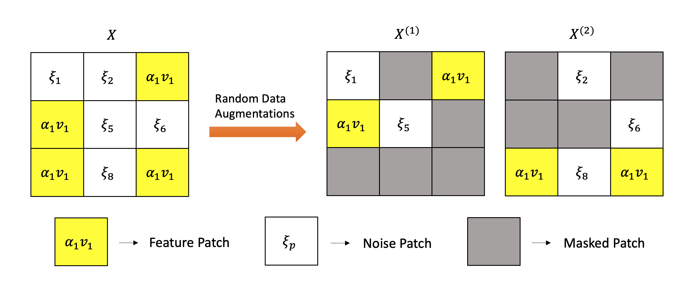
We denote 𝒮⁡(X)={p:zp​(X)≠0}⊆[P]\mathcal{S}(X)=\{p:z_{p}(X)\neq 0\}\subseteq[P] as the set of feature patches and assume zp​(X)=zp′​(X)∈{0,±αℓ},∀p,p′∈[P]z_{p}(X)=z_{p^{\prime}}(X)\in\{0,\pm\alpha_{\ell}\},\forall p,p^{\prime}\in[P], i.e., all feature patches have the same direction of vℓv_{\ell} within the same XX. We assume P=𝗉𝗈𝗅𝗒𝗅𝗈𝗀⁡(d)P=\mathsf{polylog}(d), S⁡(X)≡P0=Θ⁡(log⁡d)S(X)\equiv P_{0}=\Theta(\log d) for every XX. The assumption of ξp\xi_{p} will be given in Assumption 3.3. An intuitive illustration is given in Figure 6.

Strong and weak features.

We pick α1=2polyloglog​(d)\alpha_{1}=2^{\textsf{polyloglog}(d)} and α2=α1/𝗉𝗈𝗅𝗒𝗅𝗈𝗀⁡(d)\alpha_{2}=\alpha_{1}/\mathsf{polylog}(d). Hence v1v_{1} is the strong feature and v2v_{2} is the weak feature, and we want the learner network to learn both v1,v2v_{1},v_{2} (but by different neurons) as their learning goal. This is a simplification of the real scenario where features show up in multiple patches of the images, while noises are local and roughly independent across different patches. Intuitively, we can think of the strong features in a dataset are the ones that show up more frequently or with larger magnitude, and weak features as those that show up rarely or with smaller magnitude, which is the common case in any practical dataset.

Refer to caption
Figure 6: Illustration of the data distribution and data augmentations. Each data is equipped with a feature, either v1v_{1} or v2v_{2}, and contains a lot of noise patches. After the data augmentations, the positive pair (X(1),X(2))(X^{(1)},\,X^{(2)}) is constructed by randomly masking out half of non-overlapping patches for each positive sample. The reason for constructing positive pair with non-overlapping patches is because of the strong noise assumption we made in Assumption 3.3 and the feature decoupling principle in [88].
Remark 3.2.

Our analysis can be easily generalized to settings of either (1) when α1=α2\alpha_{1}=\alpha_{2} but the sampling of ℓ∈[2]\ell\in[2] is of non-equal probability (i.e., dataset imbalance setting); or (2) when the two features always co-occur in the same sample but not of the same strength. But we still require α1,α2≫𝗉𝗈𝗅𝗒𝗅𝗈𝗀⁡(d)\alpha_{1},\alpha_{2}\gg\mathsf{polylog}(d) to simplify the analysis.

Assumption 3.3 (noise).

Denoting V=span⁡(v1,v2)V=\mathrm{span}(v_{1},v_{2}), we assume ξp∈V⟂\xi_{p}\in V^{\perp} is independent for each p∈[P]∖S⁡(X)p\in[P]\setminus S(X), where X=(Xp)p∈[P]∼𝒟X=(X_{p})_{p\in[P]}\sim\mathcal{D}, and:

  1. 1.

    For any unit vector u∈V⟂u\in V^{\perp}, 𝔼⁡[⟨ξp,u⟩]=0\mathbb{E}[\langle\xi_{p},u\rangle]=0, and 𝔼⁡[⟨ξp,u⟩6]=σ6\mathbb{E}[\langle\xi_{p},u\rangle^{6}]=\sigma^{6} for some σ=Θ⁡(1)\sigma=\Theta(1);

  2. 2.

    It holds for some ϱ∈[0,1dΩ⁡(1)]\varrho\in[0,\frac{1}{d^{\Omega(1)}}] it holds |𝔼⁡[⟨u1,ξp⟩3​⟨u2,ξp⟩3]|≤ϱ|\mathbb{E}[\langle u_{1},\xi_{p}\rangle^{3}\langle u_{2},\xi_{p}\rangle^{3}]|\leq\varrho and |𝔼⁡[⟨u1,ξp⟩5​⟨u2,ξp⟩]|≤ϱ|\mathbb{E}[\langle u_{1},\xi_{p}\rangle^{5}\langle u_{2},\xi_{p}\rangle]|\leq\varrho for any two vectors u1,u2∈ℝdu_{1},u_{2}\in\mathbb{R}^{d} that are orthogonal to each other.

Remark 3.4.

A simple example of our noise ξp\xi_{p} is the spherical Gaussian noise in V⟂V^{\perp}. Our Assumption 3.3b ensures that the prediction head cannot be used to cancel the noise correlation between different neurons. We point out that the features in our data can be learned via clustering, but we emphasize that we do not intend to compare our algorithm with any clustering method in this setting since our goal is to study how the prediction head helps in learning the features.

3.1 Learner Network

Following the SimSiam framework, the online and target network share the same encoder network in our setting, as explained in Section 2. We consider the base encoder network ff as a simple convolutional neural network: Let W=(w1,…,wm)∈ℝd×mW=(w_{1},\dots,w_{m})\in\mathbb{R}^{d\times m} be the weight matrix, where wi∈ℝdw_{i}\in\mathbb{R}^{d}, the encoder network ff is defined by

fj​(X):=∑p∈[P]σ⁡(⟨wj,Xp⟩),∀j∈[m]\displaystyle\textstyle f_{j}(X):=\sum_{p\in[P]}\sigma(\langle w_{j},X_{p}\rangle),\qquad\forall j\in[m]

Here we use the cubic activation function σ⁡(z)=z3\sigma(z)=z^{3}, as polynomial activations are standard in literatures of deep learning theory [9, 35, 53, 2, 55, 23] and also has comparable performance in practice [2]. The (identity initialized) prediction head is defined as a matrix E=[Ei,j](i,j)∈[m]2E=[E_{i,j}]_{(i,j)\in[m]^{2}} with Ei,i≡1,i∈[m]E_{i,i}\equiv 1,i\in[m], where only the the off-diagonals Ei,j,i≠jE_{i,j},i\neq j are trainable parameters. The online network F~\widetilde{F} is defined by: given j∈[m]j\in[m], we let Fj​(X):=fj​(X)+∑r≠jEj,r​fr​(X)F_{j}(X):=f_{j}(X)+\sum_{r\neq j}E_{j,r}f_{r}(X), and

F~j​(X)\displaystyle\textstyle\widetilde{F}_{j}(X) :=𝖡𝖭(Fj(X))=𝖡𝖭[∑p∈[P](σ(⟨wj,Xp⟩)+∑r≠jEj,rσ(⟨wr,Xp⟩)]\displaystyle:=\mathsf{BN}\left(F_{j}(X)\right)=\mathsf{BN}\Bigg[\sum_{p\in[P]}\Big(\sigma(\langle w_{j},X_{p}\rangle)+\sum_{r\neq j}E_{j,r}\sigma(\langle w_{r},X_{p}\rangle\Big)\Bigg]

where the batch normalization 𝖡𝖭\mathsf{BN} here11 1 We use batch normalization as a output-normalization method, rather than for the supposed implicit negative term effects as disproved in Richemond et al. 2020. is defined as follows: Given a batch of inputs {zi}i∈[N]\{z_{i}\}_{i\in[N]},

𝖡𝖭⁡(zi):=zi−1N​∑i∈[N]zi1N​∑i∈[N]zi2−(1N​∑i∈[N]zi)2\displaystyle\mathsf{BN}(z_{i}):=\frac{z_{i}-\frac{1}{N}\sum_{i\in[N]}z_{i}}{\sqrt{\frac{1}{N}\sum_{i\in[N]}z_{i}^{2}-\left(\frac{1}{N}\sum_{i\in[N]}z_{i}\right)^{2}}} (3.1)

And the target network GG is defined as follows: Given j∈[m]j\in[m]

G~j​(X):=𝖡𝖭⁡(Gj​(X))=𝖡𝖭⁡[∑p∈[P]σ⁡(⟨wj,Xp⟩)]\displaystyle\widetilde{G}_{j}(X):=\mathsf{BN}\left(G_{j}(X)\right)=\mathsf{BN}\Bigg[\sum_{p\in[P]}\sigma(\langle w_{j},X_{p}\rangle)\Bigg]

3.2 Training Algorithm

Algorithm 1 Training Algorithm
1: data distribution 𝒟\mathcal{D}, objective L𝒮L_{\mathcal{S}} (3.3), networks F~,G~\widetilde{F},\widetilde{G}, hyper-parameters T,N,η,ηE,mT,N,\eta,\eta_{E},m, and a bool variable 𝖳𝗋𝖺𝗂𝗇𝖯𝗋𝖾𝖽𝖧𝖾𝖺𝖽=𝖳𝗋𝗎𝖾\mathsf{TrainPredHead}=\mathsf{True}.
2: Initialize wj(0)∼𝒩⁡(0,Id/d)w_{j}^{(0)}\sim\mathcal{N}(0,I_{d}/d) ∀j∈[m]\forall j\in[m] i.i.d., and E(0)=ImE^{(0)}=I_{m};
3: for t∈{0,1,2,⋯,T−1}t\in\{0,1,2,\cdots,T-1\} do
4:   Sample X(t,i)←(Xp(t,i))p∈[P]∼𝒟,∀i∈[N]X^{(t,i)}\leftarrow(X_{p}^{(t,i)})_{p\in[P]}\sim\mathcal{D},\forall i\in[N] i.i.d.;
5:   Sample {𝒫(t,i)}i∈[N]\{\mathcal{P}^{(t,i)}\}_{i\in[N]} i.i.d., and obtain 𝒮t←{X(t,i,1),X(t,i,2)}i∈[N]\mathcal{S}_{t}\leftarrow\{X^{(t,i,1)},X^{(t,i,2)}\}_{i\in[N]} via data augmentations
X(t,i,1)←(Xp(t,i)​𝟙p∈𝒫(t,i))p∈[P],X(t,i,2)←(Xp(t,i)​𝟙p∉𝒫(t,i))p∈[P];\displaystyle X^{(t,i,1)}\leftarrow(X_{p}^{(t,i)}\mathds{1}_{p\in\mathcal{P}^{(t,i)}})_{p\in[P]},\qquad X^{(t,i,2)}\leftarrow(X_{p}^{(t,i)}\mathds{1}_{p\notin\mathcal{P}^{(t,i)}})_{p\in[P]};
6:   Perform stochastic gradient descent step to W(t)=(wj(t))j∈[m]W^{(t)}=(w_{j}^{(t)})_{j\in[m]} by
wj(t+1)\displaystyle w_{j}^{(t+1)} ←wj(t)−η​∇wjL𝒮t​(W(t),E(t));\displaystyle\leftarrow w_{j}^{(t)}-\eta\nabla_{w_{j}}L_{\mathcal{S}_{t}}(W^{(t)},E^{(t)});
7:   if 𝖳𝗋𝖺𝗂𝗇𝖯𝗋𝖾𝖽𝖧𝖾𝖺𝖽=𝖳𝗋𝗎𝖾\mathsf{TrainPredHead}=\mathsf{True} then update the off diagonal of prediction head E(t)E^{(t)} by
Ei,i(t+1)←1,Ei,j(t+1)←Ei,j(t)−ηE∇Ei,jL𝒮t(W(t),E(t)),∀j≠i,i,j∈[m];\displaystyle E_{i,i}^{(t+1)}\leftarrow 1,\quad E_{i,j}^{(t+1)}\leftarrow E_{i,j}^{(t)}-\eta_{E}\nabla_{E_{i,j}}L_{\mathcal{S}_{t}}(W^{(t)},E^{(t)}),\quad\forall j\neq i,\ i,j\in[m];
8:   else keep E(t+1)=ImE^{(t+1)}=I_{m}.
9:   end if
10: end for

Data augmentation.

We use a very simple data augmentation: for each data X=(Xp)p∈[P]X=(X_{p})_{p\in[P]}, we randomly and uniformly sample half of the patches 𝒫⊆[P]\mathcal{P}\subseteq[P] to generate two samples (which is the so-called positive pair in contrastive learning):

X(1)=(Xp​𝟙p∈𝒫)p∈[P],X(2)=(Xp​𝟙p∉𝒫)p∈[P]\displaystyle X^{(1)}=(X_{p}\mathds{1}_{p\in\mathcal{P}})_{p\in[P]},\quad X^{(2)}=(X_{p}\mathds{1}_{p\notin\mathcal{P}})_{p\in[P]} (3.2)

An intuitive illustration is given in Figure 6. Our data augmentation approach is similar to the common cropping augmentation used in contrastive learning [22, 79] and the patch masking strategy in generative pretraining [16, 43] and NLP pretraining [30]. It is also analogous to the data augmentations being studied in theoretical literatures [88, 49, 61] of self-supervised learning, especially the RandomMask augmentation in [88].

Non-contrastive loss function.

Now we define the loss function as follows: we sample NN data points {Xi}i∈[N],Xi∼i.i.d.𝒟\{X_{i}\}_{i\in[N]},X_{i}\stackrel{{\scriptstyle\mathrm{i.i.d.}}}{{\sim}}\mathcal{D} and apply our data augmentation (3.2) to obtain 𝒮={X(i,1),X(i,2)}i∈[N]\mathcal{S}=\{X^{(i,1)},X^{(i,2)}\}_{i\in[N]}. Now we define

L𝒮​(W,E)\displaystyle L_{\mathcal{S}}(W,E) :=1N∑i∈[N]‖F~(X(i,1))−𝖲𝗍𝗈𝗉𝖦𝗋𝖺𝖽[G~(X(i,2)])‖22\displaystyle:=\frac{1}{N}\sum_{i\in[N]}\left\|\widetilde{F}(X^{(i,1)})-\mathsf{StopGrad}[\widetilde{G}(X^{(i,2)}])\right\|_{2}^{2} (3.3)
=2−1N​∑i∈[N]⟨F~​(X(i,1)),𝖲𝗍𝗈𝗉𝖦𝗋𝖺𝖽⁡[G~​(X(i,2))]⟩\displaystyle=2-\frac{1}{N}\sum_{i\in[N]}\langle\widetilde{F}(X^{(i,1)}),\mathsf{StopGrad}[\widetilde{G}(X^{(i,2)})]\rangle

where the 𝖲𝗍𝗈𝗉𝖦𝗋𝖺𝖽\mathsf{StopGrad} operator detach gradient computation of the target network G~​(⋅)\widetilde{G}(\cdot). This form of objective (3.3) is first defined in Grill et al. 2020 and is equivalent to (2.3) in Chen and He 2021 when F~\widetilde{F} and G~\widetilde{G} share the same encoder network f⁡(⋅)f(\cdot) and their outputs are normalized.

Intuition of the data augmentation.

Our data augmentation is an analog of the the standard cropping data augmentation. In Definition 3.1, the features v1,v2v_{1},v_{2} appear in multiple patches, but the noises are independent across different patches (see Figure 6). As our data augmentation produces positive pairs with non-overlapping patches, learning to emphasize noises cannot align the representations of the positive pair, but learning either one of the features ϕ⁡(X)=∑pσ⁡(⟨v1,Xp⟩)\phi(X)=\sum_{p}\sigma(\langle v_{1},X_{p}\rangle) or ϕ⁡(X)=∑pσ⁡(⟨v2,Xp⟩)\phi(X)=\sum_{p}\sigma(\langle v_{2},X_{p}\rangle) is sufficient. We consider learning the same feature viv_{i} in all the neurons fjf_{j} in the encoder network ff as the dimensional collapsed solution.

Initialization and hyper-parameters.

At t=0t=0, we initialize WW and EE as Wi,j(0)∼𝒩⁡(0,1d)W_{i,j}^{(0)}\sim\mathcal{N}(0,\frac{1}{d}) and E(0)=ImE^{(0)}=I_{m} and we only train the off-diagonal entries of E(t)E^{(t)}. For the simplicity of analysis, we let m=2m=2, which suffices to illustrate our main message. For the learning rates, we let η∈(0,1𝗉𝗈𝗅𝗒⁡(d)]\eta\in(0,\frac{1}{\mathsf{poly}(d)}] be sufficiently small and ηE∈[ηα1O⁡(1),η𝗉𝗈𝗅𝗒𝗅𝗈𝗀⁡(d)]\eta_{E}\in[\frac{\eta}{\alpha_{1}^{O(1)}},\frac{\eta}{\mathsf{polylog}(d)}], which is smaller than η\eta22 2 We conjecture that by modifying certain assumptions for the noise (especially by allowing the noise to span the feature subspace VV), one can prove a similar result for the case ηE=η\eta_{E}=\eta..

Optimization algorithm

Given the data augmentation and the loss function, we perform (stochastic) gradient descent on the training objective (3.3) as follows: at each iteration t=0,…,T−1t=0,\dots,T-1, we sample a new batch of augmented data 𝒮t={X(t,i,1),X(t,i,2)}i∈[N]\mathcal{S}_{t}=\{X^{(t,i,1)},X^{(t,i,2)}\}_{i\in[N]} and update

W(t+1)=W(t)−η∇WL𝒮t(W(t),E(t)),Ei,j(t+1)=Ei,j(t)−ηE∇Ei,jL𝒮t(W(t),E(t)),∀i≠j,i,j∈[m]\displaystyle W^{(t+1)}=W^{(t)}-\eta\nabla_{W}L_{\mathcal{S}_{t}}(W^{(t)},E^{(t)}),\quad E_{i,j}^{(t+1)}=E_{i,j}^{(t)}-\eta_{E}\nabla_{E_{i,j}}L_{\mathcal{S}_{t}}(W^{(t)},E^{(t)}),\ \ \forall i\neq j,\,i,j\in[m]

If we do not train the prediction head, we just simply keep E(t)≡ImE^{(t)}\equiv I_{m}. We summarize our algorithm in Algorithm 1.

4 Statements of Main Results

In this section, we shall present our main theoretical results on the mechanism of learning the prediction head in non-contrastive learning. To measure the correlation between neurons, we introduce the following notion: letting

𝐕𝐚𝐫⁡(ψ⁡(X)):=𝔼X∼𝒟​[(ψ⁡(X)−𝔼⁡[ψ⁡(X)])2]\displaystyle\mathbf{Var}(\psi(X)):=\mathbb{E}_{X\sim\mathcal{D}}[(\psi(X)-\mathbb{E}[\psi(X)])^{2}]

be the variance of any function ψ\psi of X∼𝒟X\sim\mathcal{D}, we denote the correlation 𝐂𝐨𝐫𝐫⁡(ψ⁡(X),ψ′​(X))\mathbf{Corr}(\psi(X),\psi^{\prime}(X)) of any two function ψ,ψ′\psi,\psi^{\prime} over 𝒟\mathcal{D} as

𝐂𝐨𝐫𝐫⁡(ψ⁡(X),ψ′​(X)):=𝔼⁡[(ψ⁡(X)−𝔼⁡[ψ⁡(X)])​(ψ′​(X)−𝔼⁡[ψ′​(X)])]𝐕𝐚𝐫⁡(ψ⁡(X))​𝐕𝐚𝐫​(ψ′​(X))\displaystyle\mathbf{Corr}(\psi(X),\psi^{\prime}(X)):=\frac{\mathbb{E}[(\psi(X)-\mathbb{E}[\psi(X)])(\psi^{\prime}(X)-\mathbb{E}[\psi^{\prime}(X)])]}{\sqrt{\mathbf{Var}(\psi(X))}\sqrt{\mathbf{Var}(\psi^{\prime}(X))}}

Now we present the main theorem of training with a prediction head, and set m=2m=2.

Theorem 4.1 (learning with prediction head and BN, see Theorem E.2).

For every d>2d>2, let N≥𝗉𝗈𝗅𝗒⁡(d)N\geq\mathsf{poly}(d), η∈(0,1𝗉𝗈𝗅𝗒⁡(d)]\eta\in(0,\frac{1}{\mathsf{poly}(d)}] be sufficiently small, and ηE∈[ηα1O⁡(1),η𝗉𝗈𝗅𝗒𝗅𝗈𝗀⁡(d)]\eta_{E}\in[\frac{\eta}{\alpha_{1}^{O(1)}},\frac{\eta}{\mathsf{polylog}(d)}]. Then with probability 1−o⁡(1)1-o(1), after runing Algorithm 1 for T=𝗉𝗈𝗅𝗒⁡(d)/ηT=\mathsf{poly}(d)/\eta many iterations, we shall have for some ℓ∈[2]\ell\in[2]:

w1(T)=β1vℓ+ε1,w2(T)=β2v3−ℓ+ε2with|β1|,|β2|=Θ(1),∥ε1∥2,∥ε2∥2≤O~(1d)\displaystyle w_{1}^{(T)}=\beta_{1}v_{\ell}+\varepsilon_{1},\quad w_{2}^{(T)}=\beta_{2}v_{3-\ell}+\varepsilon_{2}\qquad\text{with}\quad|\beta_{1}|,|\beta_{2}|=\Theta(1),\ \|\varepsilon_{1}\|_{2},\|\varepsilon_{2}\|_{2}\leq\widetilde{O}(\frac{1}{\sqrt{d}})

Furthermore, the objective converges: 𝔼𝒮∼𝒟N​[L𝒮​(W(T),E(T))]≤𝖮𝖯𝖳+1𝗉𝗈𝗅𝗒⁡(d)≤O⁡(1log⁡d)\mathbb{E}_{\mathcal{S}\sim\mathcal{D}^{N}}[L_{\mathcal{S}}(W^{(T)},E^{(T)})]\leq\mathsf{OPT}+\frac{1}{\mathsf{poly}(d)}\leq O(\frac{1}{\log d}). Here 𝖮𝖯𝖳\mathsf{OPT} stands for the global minimum of the objective33 3 Under our data model Definition 3.1, non-overlapping data augmentation (3.2) and learner network definition, the global minimum of our objective (3.3) in population is the following quantity: 𝖮𝖯𝖳:=minW,E⁡𝔼𝒮∼𝒟N​[L𝒮​(W,E)]=2−2​𝔼⁡[|S⁡(X)∩𝒫|⋅|𝒮⁡(X)∖𝒫|]𝔼⁡[|S⁡(X)∩𝒫|2]=Θ⁡(1log⁡d)\displaystyle\mathsf{OPT}:=\min_{W,E}\mathbb{E}_{\mathcal{S}\sim\mathcal{D}^{N}}[L_{\mathcal{S}}(W,E)]=2-2\frac{\mathbb{E}[|S(X)\cap\mathcal{P}|\cdot|\mathcal{S}(X)\setminus\mathcal{P}|]}{\mathbb{E}[|S(X)\cap\mathcal{P}|^{2}]}=\Theta(\frac{1}{\log d}) .

Theorem 4.1 clearly shows the network learn all the desired features, even under huge imbalance between v1v_{1} and v2v_{2}. This leads to the following corollary.

Corollary 4.2.

Under the same hyper-parameter in Theorem 4.1, with probability 1−o⁡(1)1-o(1), after runing Algorithm 1 for T=𝗉𝗈𝗅𝗒⁡(d)/ηT=\mathsf{poly}(d)/\eta many iterations, we shall have that the learning avoids dimensional collapse:

|𝐂𝐨𝐫𝐫⁡(f1​(X),f2​(X))|≤O⁡(1d).\displaystyle|\mathbf{Corr}(f_{1}(X),f_{2}(X))|\leq O(\frac{1}{\sqrt{d}}).

In contrast, learning without the prediction head will result in learning only the strong feature v1v_{1} in both neurons, which creates strong correlations between any two neurons. Learning v2v_{2} in this case cost at least Ω⁡(α1/α2)≫𝗉𝗈𝗅𝗒𝗅𝗈𝗀⁡(d)\Omega(\alpha_{1}/\alpha_{2})\gg\mathsf{polylog}(d) many neurons, as shown below.

Theorem 4.3 (learning without prediction head but with BN, see Theorem F.1).

Let N≥𝗉𝗈𝗅𝗒⁡(d)N\geq\mathsf{poly}(d), η=o⁡(1)\eta=o(1) and the number of neurons m=o⁡(α1/α2)m=o(\alpha_{1}/\alpha_{2}) be any positive integer. Then with probability 1−o⁡(1)1-o(1), after runing Algorithm 1 with 𝖳𝗋𝖺𝗂𝗇𝖯𝗋𝖾𝖽𝖧𝖾𝖺𝖽=𝖥𝖺𝗅𝗌𝖾\mathsf{TrainPredHead}=\mathsf{False} for T=𝗉𝗈𝗅𝗒⁡(d)/ηT=\mathsf{poly}(d)/\eta many iterations, we shall have:

wj(T)=βj​v1+εjwith|βj|=Θ⁡(1),‖εj‖2≤O~​(1d)\displaystyle w_{j}^{(T)}=\beta_{j}v_{1}+\varepsilon_{j}\qquad\text{with}\quad|\beta_{j}|=\Theta(1),\ \|\varepsilon_{j}\|_{2}\leq\widetilde{O}(\frac{1}{\sqrt{d}}) for all j∈[m]j\in[m]

Furthermore, the objective converges: 𝔼𝒮∼𝒟N​[L𝒮​(W(T),E(T))]≤𝖮𝖯𝖳+1𝗉𝗈𝗅𝗒⁡(d)≤O⁡(1log⁡d)\mathbb{E}_{\mathcal{S}\sim\mathcal{D}^{N}}[L_{\mathcal{S}}(W^{(T)},E^{(T)})]\leq\mathsf{OPT}+\frac{1}{\mathsf{poly}(d)}\leq O(\frac{1}{\log d}). This means the collapsed solution also reaches the global minimum of the objective.

Note that since we have used BN as our output normalization instead of ℓ2\ell_{2}-norm, the learner is immune to complete collapse and must have a certain variance in the outputs. Immediately, we have the following corollary.

Corollary 4.4.

Under the same hyper-parameter in Theorem 4.3, with probability 1−o⁡(1)1-o(1), after runing Algorithm 1 with 𝖳𝗋𝖺𝗂𝗇𝖯𝗋𝖾𝖽𝖧𝖾𝖺𝖽=𝖥𝖺𝗅𝗌𝖾\mathsf{TrainPredHead}=\mathsf{False} for T=𝗉𝗈𝗅𝗒⁡(d)/ηT=\mathsf{poly}(d)/\eta many iterations, we shall have dimensional collapse:

|𝐂𝐨𝐫𝐫⁡(fi​(X),fj​(X))|≥1−O⁡(1d),for all i,j∈[m].\displaystyle|\mathbf{Corr}(f_{i}(X),f_{j}(X))|\geq 1-O(\frac{1}{\sqrt{d}}),\qquad\text{for all $i,j\in[m]$.}
Remark 4.5.

Note that since we have used BN as our output normalization instead of ℓ2\ell_{2}-norm, the learner is regularized to avoid complete collapse and must have a certain variance in its neurons. It is easier to obtain a complete collapse result when the network has ℓ2\ell_{2}-normalized outputs and there is a low-variance feature (but not of smaller magnitude) in the data set, which we refrain from proving here.

How does using the prediction head or not create such a difference in features learned by the non-contrastive methods? We shall give some intuitions by digging through the training process and separately discuss the four phases of the training process.

5 The Four Phases of the Learning Process

Refer to caption
(a) Identity-initialized (trainable) prediction head
Refer to caption
(b) Learning without prediction head
Figure 7: The feature learning process over synthetic data. When trained with the prediction head, after the strong feature is learned in the faster learning neuron, the weak feature can be learned in the slower learning neuron. When trained without the prediction head, both neurons will learn the strong feature and ignore the weak feature.

We divide the complete training process into four phases: phase I for learning the stronger feature, phase II for the substitution effect, phase III for the acceleration effect, and the end phase for convergence. The first three phases explain how the prediction head can help learn the base encoder network, and the last phase of the training explains why the off-diagonal entries often shrink in the later stage of training.

5.1 Phase I: Learning the Stronger Feature

At the beginning of training, the stronger feature v1v_{1} enjoys a much larger gradient as opposed to the weaker feature v2v_{2}, so naturally, v1v_{1} will be learned first. However, if for both neurons f1,f2f_{1},f_{2} the speed of learning v1v_{1} is the same, then we cannot argue the difference between them and will not be able to show the substitution from either one to another. Indeed, let us assume at initialization, the neuron OPENf1​(⋅))f_{1}(\cdot)) won the jackpot of having larger signal-to-noise ratio of feature ⟨wj(0),v1⟩\langle w_{j}^{(0)},v_{1}\rangle, then we can show the following result under our setting.

Lemma 5.1 (learning the stronger feature, formal statement see Lemma B.13).

After T1=d2+o⁡(1)/ηT_{1}=d^{2+o(1)}/\eta many iterations, the feature v1v_{1} in neuron f1f_{1} will be learn to ⟨w1(T1),v1⟩=Ω⁡(1)\langle w_{1}^{(T_{1})},v_{1}\rangle=\Omega(1), while all other features ⟨wj(T1),vℓ⟩=o⁡(1)\langle w_{j}^{(T_{1})},v_{\ell}\rangle=o(1) for (j,ℓ)≠(1,1)(j,\ell)\neq(1,1) are small. And the prediction head ‖E(T1)−I2‖2≤d−Ω⁡(1)\|E^{(T_{1})}-I_{2}\|_{2}\leq d^{-\Omega(1)} is still close to the initialization.

In this phase, the prediction head has not come into play. The substitution effect can only happen after the feature v1v_{1} in neuron f1f_{1} is learned to a certain degree, and neuron f2f_{2} remains largely unlearned.

5.2 Phase II: The Substitution Effect

To illustrate the substitution effect, let us keep assuming that neuron w1(t)w_{1}^{(t)} has already learned some significant amount of the strong feature v1v_{1}, say w1(t)=β1​v1+𝑟𝑒𝑠𝑖𝑑𝑢𝑎𝑙w_{1}^{(t)}=\beta_{1}v_{1}+\mathit{residual} with |β1|=Ω⁡(‖𝑟𝑒𝑠𝑖𝑑𝑢𝑎𝑙‖)|\beta_{1}|=\Omega(\|\mathit{residual}\|). When this happens, we have the following result: (recall fj​(⋅),j∈[2]f_{j}(\cdot),j\in[2] are the neurons of the base encoder network)

Lemma 5.2 (substitution effect, formal statement see Lemma C.8).

After |⟨w1(t),v1⟩|=Ω⁡(1)|\langle w_{1}^{(t)},v_{1}\rangle|=\Omega(1) in O⁡(d2+o⁡(1)/η)O(d^{2+o(1)}/\eta) iterations (as shown by Lemma B.13), for much shorter time than learning ⟨w1(t),v1⟩\langle w_{1}^{(t)},v_{1}\rangle, we shall have |E2,1(t)||E_{2,1}^{(t)}| increasing until |E2,1(t)​f1​(X(1))|≫|f2​(X(1))||E_{2,1}^{(t)}f_{1}(X^{(1)})|\gg|f_{2}(X^{(1)})| when XX is equipped with feature v1v_{1}. In other words, E2,1(t)​f1​(X(1))E_{2,1}^{(t)}f_{1}(X^{(1)}) is a substitute for the feature v1v_{1} that should be learned by f2f_{2}.

Intuition of the substitution effect.

After the stronger feature is learned in neuron f1f_{1}, the optimal way to align two positive representations F2​(X(1)),G2​(X(2))F_{2}(X^{(1)}),G_{2}(X^{(2)}) is no longer learning features in weight w2w_{2}, but use the prediction head to “borrow” the features in f1f_{1} and incorporate them into F2F_{2}. This is how the substitution effect happens when trained with a prediction head.

Proof sketch for Lemma 5.2.

Indeed, let us look at the learning of E2,1(t)E_{2,1}^{(t)}. In this phase, w2(t)w_{2}^{(t)} and E2,1(t)E_{2,1}^{(t)} are roughly learned to maximize the following quantity:

F~2​(X(1))⋅G~2​(X(2))\displaystyle\textstyle\widetilde{F}_{2}(X^{(1)})\cdot\widetilde{G}_{2}(X^{(2)}) ∝(f2​(X(1))+E2,1(t)​f1​(X(1)))×f2​(X(2))\displaystyle\propto\big(f_{2}(X^{(1)})+E_{2,1}^{(t)}f_{1}(X^{(1)})\big)\times f_{2}(X^{(2)})
≈∑ℓ∈[2]αℓ6​(⟨w2(t),vℓ⟩6+E2,1(t)⋅⟨w1(t),vℓ⟩3⋅⟨w2(t),vℓ⟩3)\displaystyle\approx\textstyle\sum_{\ell\in[2]}\alpha_{\ell}^{6}\Big(\langle w_{2}^{(t)},v_{\ell}\rangle^{6}+E_{2,1}^{(t)}\cdot\langle w_{1}^{(t)},v_{\ell}\rangle^{3}\cdot\langle w_{2}^{(t)},v_{\ell}\rangle^{3}\Big)

As the neuron f1​(⋅)f_{1}(\cdot) is already learned with feature v1v_{1}, in order to maximize the RHS, we can either try to maximize ∑ℓ∈[2]⟨w2(t),vℓ⟩6\sum_{\ell\in[2]}\langle w_{2}^{(t)},v_{\ell}\rangle^{6}, or to maximize E2,1(t)​⟨w1(t),v1⟩3⋅⟨w2(t),v1⟩3≈E2,1(t)​⟨w2(t),v1⟩3E_{2,1}^{(t)}\langle w_{1}^{(t)},v_{1}\rangle^{3}\cdot\langle w_{2}^{(t)},v_{1}\rangle^{3}\approx E_{2,1}^{(t)}\langle w_{2}^{(t)},v_{1}\rangle^{3}. In this case, the more efficient choice is to learn |E2,1(t)||E_{2,1}^{(t)}| to substitute for maximizing ⟨w2(t),vℓ⟩3\langle w_{2}^{(t)},v_{\ell}\rangle^{3}. Actually, because of the high signal-to-noise ratio of learning w2(t)w_{2}^{(t)} than E2,1(t)E_{2,1}^{(t)}, feature ⟨w2(t),vℓ⟩\langle w_{2}^{(t)},v_{\ell}\rangle is learned with slower pace than E2,1(t)E_{2,1}^{(t)}, so that Lemma 5.2 can be shown.

5.3 Phase III: The Acceleration Effect

After the substitution of v1v_{1} in F2F_{2}, our concern is, whether or not w2(t)w_{2}^{(t)} will learn v2v_{2} and only v2v_{2} eventually, so that we can obtain a diverse representation? The answer is yes, as we summarize in the following lemma.

Lemma 5.3 (acceleration effect, formal statement see Lemma D.8).

After E2,1(t)E_{2,1}^{(t)} is learned in Lemma 5.2, learning v2v_{2} in w2(t)w_{2}^{(t)} will be much faster than v1v_{1}, until ‖w2(t)−β2​v2‖≤o⁡(1)\|w_{2}^{(t)}-\beta_{2}v_{2}\|\leq o(1) for some β2=Θ⁡(1)\beta_{2}=\Theta(1).

The acceleration effect is caused by the interactions between the prediction head, the stop gradient operation, and the normalization method (which in this case is the batch normalization). We shall explain these interactions with insights from our theoretical analyses below.

What is the role of the stop-gradient?

Thanks to the StopGrad operation, when we compute the gradient −∇w2F2(X(1))⋅𝖲𝗍𝗈𝗉𝖦𝗋𝖺𝖽[G2(X(2))]-\nabla_{w_{2}}F_{2}(X^{(1)})\cdot\mathsf{StopGrad}[G_{2}(X^{(2)})] to learn f2f_{2}, this negative gradient will only try to maximize f2​(X(1))⋅f2​(X(2))f_{2}(X^{(1)})\cdot f_{2}(X^{(2)}), rather than to maximize f2​(X(2))⋅F2​(X(1))f_{2}(X^{(2)})\cdot F_{2}(X^{(1)}). This is because the stop-gradient is on GG not on FF: while F2F_{2} has a large component of v1v_{1} borrowed from f1f_{1} using EE, G2G_{2} does not have this component. So the gradient of F2F_{2} is to align with the features in G2G_{2} that does not contain many v1v_{1}, while the gradient of G2G_{2} is to aligned with the features in F2F_{2} that contains a lot of v1v_{1}. Thus the stop gradient on GG help ignore the feature borrowed from f1f_{1} using prediction head EE and ensures the slower learning neuron f2f_{2} will focus on learning feature v2v_{2}.

What is the role of the output normalization?

Again due to the 𝖲𝗍𝗈𝗉𝖦𝗋𝖺𝖽\mathsf{StopGrad} operation, the gradient of F~2\widetilde{F}_{2} is taken with respect to the ratio f2​(X(1))/𝐕𝐚𝐫⁡[F2​(X(1))]f_{2}(X^{(1)})/\sqrt{\mathbf{Var}[F_{2}(X^{(1)})]}. As gradient descent tries to maximize this ratio, a direct computation gives

∇w2f2​(X(1))𝐕𝐚𝐫⁡(F2​(X(1)))=∇w2f2​(X(1))⋅𝐕𝐚𝐫⁡(F2​(X(1)))−f2​(X(1))⋅∇w2𝐕𝐚𝐫​(F2​(X(1)))𝐕𝐚𝐫​(F2​(X(1)))3/2\displaystyle\nabla_{w_{2}}\frac{f_{2}(X^{(1)})}{\sqrt{\mathbf{Var}(F_{2}(X^{(1)}))}}=\frac{\nabla_{w_{2}}f_{2}(X^{(1)})\cdot\mathbf{Var}(F_{2}(X^{(1)}))-f_{2}(X^{(1)})\cdot\nabla_{w_{2}}\mathbf{Var}(F_{2}(X^{(1)}))}{\mathbf{Var}(F_{2}(X^{(1)}))^{3/2}}

From some calculation, we can obtain the above gradient is proportional to

∑ℓ∈[2]([E2,1(t)​⟨w1(t),v3−ℓ⟩3]2+𝐕𝐚𝐫⁡[f2​(X(1))])​⟨∇w2f2​(X(1)),vℓ⟩​vℓ\displaystyle\textstyle\sum_{\ell\in[2]}\Big([E_{2,1}^{(t)}\langle w_{1}^{(t)},v_{3-\ell}\rangle^{3}]^{2}+\mathbf{Var}[f_{2}(X^{(1)})]\Big)\langle\nabla_{w_{2}}f_{2}(X^{(1)}),v_{\ell}\rangle v_{\ell}

which borrow the substituted feature v3−ℓv_{3-\ell} from f1​(⋅)f_{1}(\cdot) to adjust the gradient of vℓv_{\ell} in f2​(⋅)f_{2}(\cdot), via the prediction head E2,1(t)E_{2,1}^{(t)}. Without the output normalization, the learning of v1v_{1} will dominate that of v2v_{2} even when we train the prediction head.

Proof sketch for Lemma 5.3.

At this stage, when we are updating the weights of w2(t)w_{2}^{(t)}, we are simultaneuously maximizing f2​(X(1))⋅f2​(X(2))f_{2}(X^{(1)})\cdot f_{2}(X^{(2)}) and also minimizing the normalizing constants 𝐕𝐚𝐫⁡[F2​(X(1))]\sqrt{\mathbf{Var}[F_{2}(X^{(1)})]}. This two goals are in slight conflict because of the normalization, and by careful calculation the gradients are roughly given by (interpreting the expectation as empirical)

⟨−∇w2L𝒮,vℓ⟩\displaystyle\textstyle\langle-\nabla_{w_{2}}L_{\mathcal{S}},v_{\ell}\rangle ∝𝔼⁡[([E2,1(t)​⟨w1(t),v3−ℓ⟩3]2+𝐕𝐚𝐫⁡[f2​(X(1))])⋅f2​(X(2))​⟨−∇w2f2​(X(1)),vℓ⟩]\displaystyle\propto\mathbb{E}\left[\Big([E_{2,1}^{(t)}\langle w_{1}^{(t)},v_{3-\ell}\rangle^{3}]^{2}+\mathbf{Var}[f_{2}(X^{(1)})]\Big)\cdot f_{2}(X^{(2)})\langle-\nabla_{w_{2}}f_{2}(X^{(1)}),v_{\ell}\rangle\right]

Because of the learning of f1f_{1} and the substitution effect, we now knows [E2,1(t)​⟨w1(t),v3−ℓ⟩3]2[E_{2,1}^{(t)}\langle w_{1}^{(t)},v_{3-\ell}\rangle^{3}]^{2} is much larger when ℓ=2\ell=2, which accelerates the learning of v2v_{2} in w2(t)w_{2}^{(t)} to surpass that of v1v_{1} and leads to Lemma 5.3.

5.4 The End Phase: Convergence

As the weak features are learned, we have already obtained a good encoder network f⁡(⋅)f(\cdot) as shown in Theorem 4.1. The rest of our analysis is to understand what the prediction head converges to in polynomial time. Actually, our Theorem E.2 also contains the following result:

Proposition 5.4 (convergence of the prediction head, see Theorem E.2c).

After some t≥T=𝗉𝗈𝗅𝗒⁡(d)/ηt\geq T=\mathsf{poly}(d)/\eta iterations, we shall have ‖E(t)−I2‖F≤1𝗉𝗈𝗅𝗒⁡(d)\|E^{(t)}-I_{2}\|_{F}\leq\frac{1}{\mathsf{poly}(d)}.

This result also implies that after learning the weak feature v2v_{2} is complete, the off-diagonal entries of the prediction head will reverse their trajectory and converge to zero at the end of training. While we admit that only some of our real-world experiments show the convergence to zero for the off-diagonal entries of the prediction head, most of the experiments do display a rise and fall trajectory pattern of off-diagonal entries consistently.

6 Additional Related Work

Self-supervised learning

The area of self-supervised learning has evolved at a tremendous speed in recent years. It has created huge success in natural language processing [30, 89, 18] and established a paradigm where the networks are first trained on an unsupervised pretext task and then be finetuned in downstream applications. In vision, supervised pretraining had been the go-to choice until representations learned by contrastive learning [78, 42, 24, 20, 27, 28, 34, 67, 33] became dominant in many downstream tasks. Another type of self-supervised learning is the generative learning [68, 16, 43], which also gives promising results in downstream adaptations. Interesting applications such as [67, 69] also illustrate the power of contrastive learning in multiple domains.

Theory of self-supervised learning

The theoretical side of self-supervised learning developed quickly due to the success of contrastive learning, which is closely related to the methods we are studying. Since Arora et al. 2019c, lots of papers have studied the properties of contrastive learning, as mentioned in the introduction. [25, 72] discussed many interesting phenomena associated with the negative term in contrastive learning. Saunshi et al. 2022 provided pieces of evidence that contrastive loss is function class-specific rather than agnostic. Wen and Li 2021 took a feature learning view to understand contrastive learning with neural networks, which inspired our analysis in the non-contrastive setting. For generative self-supervised learning, [54, 77] provides downstream performance guarantees for generative pretrained models. [73, 87] studied the natural language tasks, where the data are sequentially structured. Liu et al. 2022 gave a recovery guarantee for tensors in generative learning under hidden Markov models. [4] analyzed multi-layer generative adversarial networks and provided an optimization guarantee for their stochastic gradient descent ascent algorithm.

Feature learning theory of deep learning

Our theoretical results are also inspired by the recent progress of the feature learning theory of neural networks [58, 59, 5, 3, 52, 93, 47]. Li et al. 2019 initiate the study of the speed difference in learning different types of features. [59] developed theory for learning two-layer neural networks over Gaussian distribution beyond the neural tangent kernel (NTK) [7, 8, 6, 32, 11]. Allen-Zhu and Li 2021 studied the origin of adversarial examples and how adversarial training help in robustify the networks. [3] tried to explain ensemble and knowledge distillation under multi-view assumptions. Techniques in this paper are built on this line of research, as the non-convex nature of these analyses allows us to describe the interaction between neural networks, optimization algorithms, and the structures of data. [1, 2] also obtained results separating deep neural networks and shallow models such as kernel methods. Before this recent progress, [80, 92, 19, 75, 31, 56, 57] also studied how shallow neural networks can learn on certain simple data distributions, but all of them focus on the supervised learning. There are also plenty of studies [76, 40, 10, 63, 50, 70, 29] on the implicit bias of optimization in deep learning, but none of their techniques can be applied to the setting of self-supervised learning.

7 Conclusion and Discussion

In this paper, we showed how the prediction head can ensure the neural network learns all the features in non-contrastive learning through theoretical investigation. Our key observation is that the prediction head can leverage two effects called substitution effect and acceleration effect during the training process. We also explained how the necessary components such as output normalization and stop-gradient operation are involved and how they interact during training. Furthermore, we proved that without the prediction head, all neurons of the neural network would focus on learning the strongest feature and result in a collapsed representation. We believe our theory, although based on a very simple setup, can provide some insights into the inner workings of non-contrastive self-supervised learning. We also believe our theoretical framework can be extended to understanding other phenomena in the practice of deep learning.

On the other hand, our results are still very preliminary, we point out the following open problems that are not addressed by this paper:

  • •

    When the output normalization is ℓ2\ell_{2}-norm instead of BN. Experiments in Figure 2 seem to suggest that there is still a gap between using ℓ2\ell_{2}-norm and BN as output normalization methods. In this case, the acceleration effect may not happen in exactly the same way as in the BN case, but we believe they share the same underlying mechanism and can be proven in theory.

  • •

    The mystery of the projection head. As our experiments in Figure 1 showed, the outputs of the projection head in the symmetric case (without the prediction head) suffer an extremely strong correlation even with batch normalization used. However, the impact on the base encoder is milder and thus the network can avoid complete collapse, shown in Figure 1 and Figure 2. It is mysterious how the projection head works in non-contrastive learning, and also how it compares to the case of contrastive learning, which has been studied by [24, 51].

  • •

    Learning non-linearly features. For the simplicity of analysis, we have assumed the features in the data set are linear. It is of interest to study whether neural networks trained by non-contrastive self-supervised learning can learn non-linear representations better than traditional learning methods such as linear regression or kernel methods, as there has been a series of papers [1, 36, 37, 2, 52] trying to understand it in the supervised setting.

In the end, we also point out that theories based on a one-hidden-layer neural network and linear data composition assumption obviously cannot explain all the phenomena in deep learning. In supervised learning, the backward feature correction [2] process is observed and theoretically proven as a mechanism for learning hierarchical feature extractors. It is an important open direction to understand how a multi-layer network can learn the complicated features in non-contrastive self-supervised learning.

8 Experiment Details

Figure 8: Framework.
Refer to caption

The framework we use in our experiments is shown in Figure 8. We use a modified version of the codebase shared by the authors of [33], and we use the same data augmentation in their implementation. All our experiments (except for Figure 5 and Figure 7) use the following architecture and hyper-parameters: we choose standard ResNet-18 as base encoder architecture, 0.0030.003 as the learning rate for Adam optimizer, a two-layer MLP with ReLU activation and 512512 hidden neurons as the projection head, an identity-initialized but diagonally froze linear matrix (with shape (64x64)) as the prediction head and a non-tracking-stats, non-affine, non-momentum BN layer as the output normalization. Our experiments in Figure 3 use the same architecture and hyper-parameters, but some runs are trained with EMA with momentum 0.990.99, with output BN replaced by ℓ2\ell_{2}-norm or using different prediction heads (such as a two-layer MLP or a linear head, with Pytorch default initialization). Evaluation in Figure 2 is by training a linear classifier on top of frozen encoder with no data augmentation.

Appendix: The Proofs

We will be working with population gradients throughout the entire appendix. Indeed, since our algorithms use fresh random samples at each iteration, one can easily obtain from standard concentration inequalities an empirical estimate of population gradients up to 1𝗉𝗈𝗅𝗒⁡(d)\frac{1}{\mathsf{poly}(d)} error with N=𝗉𝗈𝗅𝗒⁡(d)N=\mathsf{poly}(d) samples. So we can obtain the same proofs in finite sample case as long as the training ends before some T=𝗉𝗈𝗅𝗒⁡(d)/ηT=\mathsf{poly}(d)/\eta. Now we give some notations and warm-up calculations.

Appendix A Notations and Gradients

In this section, we will give some useful notations and warm-up computations for the technical proofs in subsequent sections. We summarize here the notations that will also be defined in later sections:

Notations.

We denote ℰj=𝔼⁡[⟨wj,ξp⟩6]\mathcal{E}_{j}=\mathbb{E}[\langle w_{j},\xi_{p}\rangle^{6}], ℰj,3−j=𝔼⁡[(⟨wj,ξp⟩3+Ej,3−j​⟨w3−j,ξp⟩3)2]\mathcal{E}_{j,3-j}=\mathbb{E}\left[(\langle w_{j},\xi_{p}\rangle^{3}+E_{j,3-j}\langle w_{3-j},\xi_{p}\rangle^{3})^{2}\right], and

C0\displaystyle C_{0} =𝔼⁡[|S⁡(X)∩𝒫|⋅|𝒮⁡(X)∖𝒫|]2,\displaystyle=\frac{\mathbb{E}[|S(X)\cap\mathcal{P}|\cdot|\mathcal{S}(X)\setminus\mathcal{P}|]}{2}, C1\displaystyle C_{1} =𝔼⁡[|S⁡(X)∩𝒫|2]2,\displaystyle=\frac{\mathbb{E}\left[|S(X)\cap\mathcal{P}|^{2}\right]}{2}, C2\displaystyle C_{2} =P−|S⁡(X)|,\displaystyle=P-|S(X)|,
B¯j,ℓ3\displaystyle\bar{B}_{j,\ell}^{3} =𝖲𝗍𝗈𝗉𝖦𝗋𝖺𝖽⁡[⟨wj,vℓ⟩3],\displaystyle=\mathsf{StopGrad}[\langle w_{j},v_{\ell}\rangle^{3}], Bj,ℓ\displaystyle B_{j,\ell} =⟨wj,vℓ⟩,\displaystyle=\langle w_{j},v_{\ell}\rangle, Qj\displaystyle Q_{j} =(𝔼[𝖲𝗍𝗈𝗉𝖦𝗋𝖺𝖽[Gj2(X(2))]])−1/2.\displaystyle=(\mathbb{E}[\mathsf{StopGrad}[G_{j}^{2}(X^{(2)})]])^{-1/2}.

and

Uj\displaystyle U_{j} :=𝔼⁡[Fj2​(X(1))]=∑ℓ∈[2]C1​αℓ6​(Bj,ℓ3+Ej,3−j​B3−j,ℓ3)2+C2​ℰj,3−j\displaystyle:=\mathbb{E}[F_{j}^{2}(X^{(1)})]=\textstyle\sum_{\ell\in[2]}C_{1}\alpha_{\ell}^{6}(B_{j,\ell}^{3}+E_{j,3-j}B_{3-j,\ell}^{3})^{2}+C_{2}\mathcal{E}_{j,3-j}
Hj,ℓ\displaystyle H_{j,\ell} :=C1​αℓ6​(Bj,ℓ3+Ej,3−j​B3−j,ℓ3)2+C2​ℰj,3−j,\displaystyle:=C_{1}\alpha_{\ell}^{6}(B_{j,\ell}^{3}+E_{j,3-j}B_{3-j,\ell}^{3})^{2}+C_{2}\mathcal{E}_{j,3-j},
Kj,ℓ\displaystyle K_{j,\ell} :=C1​αℓ6​(Bj,ℓ3+Ej,3−j​B3−j,ℓ3)​(Bj,3−ℓ3+Ej,3−j​B3−j,3−ℓ3)\displaystyle:=C_{1}\alpha_{\ell}^{6}(B_{j,\ell}^{3}+E_{j,3-j}B_{3-j,\ell}^{3})(B_{j,3-\ell}^{3}+E_{j,3-j}B_{3-j,3-\ell}^{3})

Moreover, we denote Φj:=Qj/Uj3/2\Phi_{j}:=Q_{j}/U_{j}^{3/2}, and (recall V:=span⁡(v1,v2)V:=\mathrm{span}(v_{1},v_{2}))

Rj:=⟨ΠV⟂​wj,wj⟩R1,2:=⟨ΠV⟂​w1,w2⟩R¯1,2:=⟨ΠV⟂​w1,w2⟩‖ΠV⟂​w1‖2​‖ΠV⟂​w2‖2\displaystyle R_{j}:=\langle\Pi_{V^{\perp}}w_{j},w_{j}\rangle\qquad R_{1,2}:=\langle\Pi_{V^{\perp}}w_{1},w_{2}\rangle\qquad\overline{R}_{1,2}:=\frac{\langle\Pi_{V^{\perp}}w_{1},w_{2}\rangle}{\|\Pi_{V^{\perp}}w_{1}\|_{2}\|\Pi_{V^{\perp}}w_{2}\|_{2}}

For any j∈[2]j\in[2], the gradient −∇wjL​(W,E)-\nabla_{w_{j}}L(W,E) can be decomposed as

−∇wjL​(W,E)\displaystyle-\nabla_{w_{j}}L(W,E) =∑ℓ∈[2](Λj,ℓ+Γj,ℓ−Υj,ℓ)​vℓ−∑(j′,ℓ)∈[2]×[2]Σj′,ℓ​∇wjℰj′,3−j′\displaystyle=\sum_{\ell\in[2]}(\Lambda_{j,\ell}+\Gamma_{j,\ell}-\Upsilon_{j,\ell})v_{\ell}-\sum_{(j^{\prime},\ell)\in[2]\times[2]}\Sigma_{j^{\prime},\ell}\nabla_{w_{j}}\mathcal{E}_{j^{\prime},3-j^{\prime}}
Λj,ℓ\displaystyle\Lambda_{j,\ell} :=C0​Φj​αℓ6​Bj,ℓ5​Hj,3−ℓ\displaystyle:=C_{0}\Phi_{j}\alpha_{\ell}^{6}B_{j,\ell}^{5}H_{j,3-\ell}
Γj,ℓ\displaystyle\Gamma_{j,\ell} :=C0​Φ3−j​E3−j,j​αℓ6​B3−j,ℓ3​Bj,ℓ2​H3−j,3−ℓ\displaystyle:=C_{0}\Phi_{3-j}E_{3-j,j}\alpha_{\ell}^{6}B_{3-j,\ell}^{3}B_{j,\ell}^{2}H_{3-j,3-\ell}
Υj,ℓ\displaystyle\Upsilon_{j,\ell} :=C0​α3−ℓ6​(Φj​Bj,3−ℓ3​Bj,ℓ2​Kj,ℓ+Φ3−j​E3−j,j​B3−j,3−ℓ3​Bj,ℓ2​K3−j,ℓ)\displaystyle:=C_{0}\alpha_{3-\ell}^{6}\left(\Phi_{j}B_{j,3-\ell}^{3}B_{j,\ell}^{2}K_{j,\ell}+\Phi_{3-j}E_{3-j,j}B_{3-j,3-\ell}^{3}B_{j,\ell}^{2}K_{3-j,\ell}\right)
Σj,ℓ\displaystyle\Sigma_{j,\ell} :=C0​C2​Φj​αℓ6​Bj,ℓ3​(Bj,ℓ3+Ej,3−j​B3−j,ℓ3)\displaystyle:=C_{0}C_{2}\Phi_{j}\alpha_{\ell}^{6}B_{j,\ell}^{3}(B_{j,\ell}^{3}+E_{j,3-j}B_{3-j,\ell}^{3})

Sometimes we need to decompose Υj,ℓ=Υj,ℓ,1+Υj,ℓ,2\Upsilon_{j,\ell}=\Upsilon_{j,\ell,1}+\Upsilon_{j,\ell,2} which is straightforward from its expression. In Section D, we further define

Ξj(t)\displaystyle\Xi_{j}^{(t)} =C0​C1​α16​α26​Φj(t)​((B1,1(t))6​(B2,2(t))6+(B2,1(t))6​(B1,2(t))6)\displaystyle=C_{0}C_{1}\alpha_{1}^{6}\alpha_{2}^{6}\Phi_{j}^{(t)}\Big((B_{1,1}^{(t)})^{6}(B_{2,2}^{(t)})^{6}+(B_{2,1}^{(t)})^{6}(B_{1,2}^{(t)})^{6}\Big)
Δj,ℓ(t)\displaystyle\Delta_{j,\ell}^{(t)} =C0​Φj(t)​αℓ6​(Bj,ℓ(t))3​(B3−j,ℓ(t))3​C2​ℰj,3−j(t)\displaystyle=C_{0}\Phi_{j}^{(t)}\alpha_{\ell}^{6}(B_{j,\ell}^{(t)})^{3}(B_{3-j,\ell}^{(t)})^{3}C_{2}\mathcal{E}_{j,3-j}^{(t)}

for the gradients of the prediction head.

A.1 Gradient Computation

Let us L⁡(W,E)L(W,E) to be the population version of the objective. Because 𝔼⁡[Fj​(X(1))]\mathbb{E}[F_{j}(X^{(1)})] and 𝔼⁡[Gj​(X(2))]\mathbb{E}[G_{j}(X^{(2)})] are both zero (which can be verified easily from the zero-mean assumptions of zp​(X)z_{p}(X) and ξp\xi_{p}), a direct computation gives:

L⁡(W,E)=2−∑j∈[2]𝔼⁡[Fj​(X(1))⋅𝖲𝗍𝗈𝗉𝖦𝗋𝖺𝖽⁡[Gj​(X(2))]]𝔼⁡[Fj2​(X(1))]​𝔼⁡[𝖲𝗍𝗈𝗉𝖦𝗋𝖺𝖽⁡[Gj2​(X(2))]]\displaystyle L(W,E)=2-\sum_{j\in[2]}\frac{\mathbb{E}[F_{j}(X^{(1)})\cdot\mathsf{StopGrad}[G_{j}(X^{(2)})]]}{\sqrt{\mathbb{E}[F_{j}^{2}(X^{(1)})]}\sqrt{\mathbb{E}[\mathsf{StopGrad}[G_{j}^{2}(X^{(2)})]]}}

We first calculate the normalizing quantity 𝔼⁡[Fj2​(X(1))]\mathbb{E}[F_{j}^{2}(X^{(1)})]:

𝔼⁡[Fj2​(X(1))]\displaystyle\mathbb{E}[F_{j}^{2}(X^{(1)})] =𝔼⁡[(∑p∈[P]σ⁡(⟨wj,Xp(1)⟩)+Ej,3−j​σ​(⟨w3−j,Xp(1)⟩))2]\displaystyle=\mathbb{E}\left[\left(\sum_{p\in[P]}\sigma(\langle w_{j},X_{p}^{(1)}\rangle)+E_{j,3-j}\sigma(\langle w_{3-j},X_{p}^{(1)}\rangle)\right)^{2}\right]
=12​∑ℓ∈[2]𝔼⁡[|S⁡(X)∩𝒫|2​αℓ6​(⟨wj,vℓ⟩3+Ej,3−j​⟨w3−j,vℓ⟩3)2]\displaystyle=\frac{1}{2}\sum_{\ell\in[2]}\mathbb{E}\left[|S(X)\cap\mathcal{P}|^{2}\alpha_{\ell}^{6}(\langle w_{j},v_{\ell}\rangle^{3}+E_{j,3-j}\langle w_{3-j},v_{\ell}\rangle^{3})^{2}\right] (Because all signal patches has the same sign within the same data)
+𝔼⁡[|𝒫∖S⁡(X)|​(⟨wj,ξp⟩3+Ej,3−j​⟨w3−j,ξp⟩3)2]\displaystyle\quad+\mathbb{E}\left[|\mathcal{P}\setminus S(X)|(\langle w_{j},\xi_{p}\rangle^{3}+E_{j,3-j}\langle w_{3-j},\xi_{p}\rangle^{3})^{2}\right] (Because noise patches are independent and have mean zero)
=∑ℓ∈[2]αℓ6​(⟨wj,vℓ⟩3+Ej,3−j​⟨w3−j,vℓ⟩3)2​𝔼⁡[|S⁡(X)∩𝒫|2]2+(P−|S⁡(X)|)​ℰj,3−j\displaystyle=\sum_{\ell\in[2]}\alpha_{\ell}^{6}(\langle w_{j},v_{\ell}\rangle^{3}+E_{j,3-j}\langle w_{3-j},v_{\ell}\rangle^{3})^{2}\frac{\mathbb{E}\left[|S(X)\cap\mathcal{P}|^{2}\right]}{2}+(P-|S(X)|)\mathcal{E}_{j,3-j}

where we let

ℰj,3−j\displaystyle\mathcal{E}_{j,3-j} =def𝔼⁡[(⟨wj,ξp⟩3+Ej,3−j​⟨w3−j,ξp⟩3)2]\displaystyle\stackrel{{\scriptstyle\text{def}}}{{=}}\mathbb{E}\left[(\langle w_{j},\xi_{p}\rangle^{3}+E_{j,3-j}\langle w_{3-j},\xi_{p}\rangle^{3})^{2}\right]
=𝔼⁡[⟨wj,ξp⟩6+2​Ej,3−j​⟨wj,ξp⟩3​⟨w3−j,ξp⟩3+Ej,3−j2​⟨w3−j,ξp⟩6]\displaystyle=\mathbb{E}\left[\langle w_{j},\xi_{p}\rangle^{6}+2E_{j,3-j}\langle w_{j},\xi_{p}\rangle^{3}\langle w_{3-j},\xi_{p}\rangle^{3}+E_{j,3-j}^{2}\langle w_{3-j},\xi_{p}\rangle^{6}\right]

On the other hand, we have

𝔼⁡[Fj​(X(1))⋅𝖲𝗍𝗈𝗉𝖦𝗋𝖺𝖽⁡[Gj​(X(2))]]\displaystyle\mathbb{E}[F_{j}(X^{(1)})\cdot\mathsf{StopGrad}[G_{j}(X^{(2)})]]
=\displaystyle=\ 𝔼⁡[(∑p∈[P]σ⁡(⟨wj,Xp(1)⟩)+Ej,3−j​σ​(⟨w3−j,Xp(1)⟩))×(∑p∈[P]σ⁡(⟨wj,Xp(2)⟩))]\displaystyle\mathbb{E}\left[\left(\sum_{p\in[P]}\sigma(\langle w_{j},X_{p}^{(1)}\rangle)+E_{j,3-j}\sigma(\langle w_{3-j},X_{p}^{(1)}\rangle)\right)\times\left(\sum_{p\in[P]}\sigma(\langle w_{j},X_{p}^{(2)}\rangle)\right)\right]
=\displaystyle=\ 12​∑ℓ∈[2]𝔼⁡[∑p∈S⁡(X)∩𝒫αℓ3​(⟨wj,vℓ⟩3+Ej,3−j​⟨w3−j,vℓ⟩3)×∑p∈S⁡(X)∖𝒫αℓ3​𝖲𝗍𝗈𝗉𝖦𝗋𝖺𝖽​[⟨wj,vℓ⟩3]]\displaystyle\frac{1}{2}\sum_{\ell\in[2]}\mathbb{E}\left[\sum_{p\in S(X)\cap\mathcal{P}}\alpha_{\ell}^{3}(\langle w_{j},v_{\ell}\rangle^{3}+E_{j,3-j}\langle w_{3-j},v_{\ell}\rangle^{3})\times\sum_{p\in S(X)\setminus\mathcal{P}}\alpha_{\ell}^{3}\mathsf{StopGrad}[\langle w_{j},v_{\ell}\rangle^{3}]\right]
=\displaystyle=\ ∑ℓ∈[2]αℓ6​(⟨wj,vℓ⟩3+Ej,3−j​⟨w3−j,vℓ⟩3)⋅𝖲𝗍𝗈𝗉𝖦𝗋𝖺𝖽⁡[⟨wj,vℓ⟩3]⋅𝔼⁡[|S⁡(X)∩𝒫|⋅|𝒮⁡(X)∖𝒫|]2\displaystyle\sum_{\ell\in[2]}\alpha_{\ell}^{6}(\langle w_{j},v_{\ell}\rangle^{3}+E_{j,3-j}\langle w_{3-j},v_{\ell}\rangle^{3})\cdot\mathsf{StopGrad}[\langle w_{j},v_{\ell}\rangle^{3}]\cdot\frac{\mathbb{E}[|S(X)\cap\mathcal{P}|\cdot|\mathcal{S}(X)\setminus\mathcal{P}|]}{2}

Now, by denoting

C0\displaystyle C_{0} =𝔼⁡[|S⁡(X)∩𝒫|⋅|𝒮⁡(X)∖𝒫|]2,\displaystyle=\frac{\mathbb{E}[|S(X)\cap\mathcal{P}|\cdot|\mathcal{S}(X)\setminus\mathcal{P}|]}{2}, C1\displaystyle C_{1} =𝔼⁡[|S⁡(X)∩𝒫|2]2,\displaystyle=\frac{\mathbb{E}\left[|S(X)\cap\mathcal{P}|^{2}\right]}{2}, C2\displaystyle C_{2} =P−|S⁡(X)|,\displaystyle=P-|S(X)|,
B¯j,ℓ3\displaystyle\bar{B}_{j,\ell}^{3} =𝖲𝗍𝗈𝗉𝖦𝗋𝖺𝖽⁡[⟨wj,vℓ⟩3],\displaystyle=\mathsf{StopGrad}[\langle w_{j},v_{\ell}\rangle^{3}], Bj,ℓ\displaystyle B_{j,\ell} =⟨wj,vℓ⟩,\displaystyle=\langle w_{j},v_{\ell}\rangle, Qj\displaystyle Q_{j} =(𝔼[𝖲𝗍𝗈𝗉𝖦𝗋𝖺𝖽[Gj2(X(2))]])−1/2.\displaystyle=(\mathbb{E}[\mathsf{StopGrad}[G_{j}^{2}(X^{(2)})]])^{-1/2}.

we denote Uj:=𝔼⁡[Fj2​(X(1))]U_{j}:=\mathbb{E}[F_{j}^{2}(X^{(1)})], where the expanded expression is

Uj=𝔼⁡[Fj2​(X(1))]=∑ℓ∈[2]C1​αℓ6​(Bj,ℓ3+Ej,3−j​B3−j,ℓ3)2+C2​ℰj,3−j\displaystyle U_{j}=\mathbb{E}[F_{j}^{2}(X^{(1)})]=\sum_{\ell\in[2]}C_{1}\alpha_{\ell}^{6}(B_{j,\ell}^{3}+E_{j,3-j}B_{3-j,\ell}^{3})^{2}+C_{2}\mathcal{E}_{j,3-j}

and we can rewrite the objective as follows

L⁡(W,E)=2−∑j∈[2]∑ℓ∈[2]Qj​C0​αℓ6​B¯j,ℓ3​(Bj,ℓ3+Ej,3−j​B3−j,ℓ3)Uj1/2\displaystyle L(W,E)=2-\sum_{j\in[2]}\sum_{\ell\in[2]}\frac{Q_{j}C_{0}\alpha_{\ell}^{6}\bar{B}_{j,\ell}^{3}(B_{j,\ell}^{3}+E_{j,3-j}B_{3-j,\ell}^{3})}{U_{j}^{1/2}} (A.1)

Now denote

Hj,ℓ\displaystyle H_{j,\ell} =C1​αℓ6​(Bj,ℓ3+Ej,3−j​B3−j,ℓ3)2+C2​ℰj,3−j,\displaystyle=C_{1}\alpha_{\ell}^{6}(B_{j,\ell}^{3}+E_{j,3-j}B_{3-j,\ell}^{3})^{2}+C_{2}\mathcal{E}_{j,3-j},
Kj,ℓ\displaystyle K_{j,\ell} =C1​αℓ6​(Bj,ℓ3+Ej,3−j​B3−j,ℓ3)​(Bj,3−ℓ3+Ej,3−j​B3−j,3−ℓ3)\displaystyle=C_{1}\alpha_{\ell}^{6}(B_{j,\ell}^{3}+E_{j,3-j}B_{3-j,\ell}^{3})(B_{j,3-\ell}^{3}+E_{j,3-j}B_{3-j,3-\ell}^{3})

It is easy to calculate

Qj−2\displaystyle Q_{j}^{-2} =𝔼⁡[𝖲𝗍𝗈𝗉𝖦𝗋𝖺𝖽⁡[Gj2​(X(2))]]\displaystyle=\mathbb{E}[\mathsf{StopGrad}[G_{j}^{2}(X^{(2)})]]
=𝔼⁡[(∑p∈[P]σ⁡(⟨wj,Xp(2)⟩))2]\displaystyle=\mathbb{E}\left[\Bigg(\sum_{p\in[P]}\sigma(\langle w_{j},X_{p}^{(2)}\rangle)\Bigg)^{2}\right]
=12​∑ℓ∈[2]αℓ6​⟨wj,vℓ⟩6​𝔼​[|S⁡(X)∩𝒫|2]+𝔼⁡[|𝒫∖S⁡(X)|​⟨wj,ξp⟩6]\displaystyle=\frac{1}{2}\sum_{\ell\in[2]}\alpha_{\ell}^{6}\langle w_{j},v_{\ell}\rangle^{6}\mathbb{E}\left[|S(X)\cap\mathcal{P}|^{2}\right]+\mathbb{E}\left[|\mathcal{P}\setminus S(X)|\langle w_{j},\xi_{p}\rangle^{6}\right]
=∑ℓ∈[2]C1​αℓ6​Bj,ℓ6+C2​ℰj\displaystyle=\sum_{\ell\in[2]}C_{1}\alpha_{\ell}^{6}B_{j,\ell}^{6}+C_{2}\mathcal{E}_{j}

where ℰj=𝔼⁡[⟨wj,ξp⟩6]\mathcal{E}_{j}=\mathbb{E}[\langle w_{j},\xi_{p}\rangle^{6}]. And thus the gradient can be computed as (notice B¯j,ℓ3=Bj,ℓ3\bar{B}_{j,\ell}^{3}=B_{j,\ell}^{3})

−∇wjL​(W,E)\displaystyle-\nabla_{w_{j}}L(W,E) =∑ℓ∈[2](C0​Qj​αℓ6​Hj,3−ℓ​Bj,ℓ5Uj3/2)​vℓ+∑ℓ∈[2](C0​Q3−j​E3−j,j​αℓ6​B3−j,ℓ3​Bj,ℓ2​H3−j,3−ℓU3−j3/2)​vℓ\displaystyle=\sum_{\ell\in[2]}\left(\frac{C_{0}Q_{j}\alpha_{\ell}^{6}H_{j,3-\ell}B_{j,\ell}^{5}}{U_{j}^{3/2}}\right)v_{\ell}+\sum_{\ell\in[2]}\left(\frac{C_{0}Q_{3-j}E_{3-j,j}\alpha_{\ell}^{6}B_{3-j,\ell}^{3}B_{j,\ell}^{2}H_{3-j,3-\ell}}{U_{3-j}^{3/2}}\right)v_{\ell}
−∑ℓ∈[2](C0​Qj​α3−ℓ6​Bj,3−ℓ3​Bj,ℓ2​Kj,ℓUj3/2+C0​Q3−j​E3−j,j​α3−ℓ6​B3−j,3−ℓ3​Bj,ℓ2​K3−j,ℓU3−j3/2)vℓ\displaystyle\quad-\sum_{\ell\in[2]}\left(\frac{C_{0}Q_{j}\alpha_{3-\ell}^{6}B_{j,3-\ell}^{3}B_{j,\ell}^{2}K_{j,\ell}}{U_{j}^{3/2}}+\frac{C_{0}Q_{3-j}E_{3-j,j}\alpha_{3-\ell}^{6}B_{3-j,3-\ell}^{3}B_{j,\ell}^{2}K_{3-j,\ell}}{U_{3-j}^{3/2}}\right)v_{\ell}
−∑j′∈[2]∑ℓ∈[2]C0​C2​Qj′​αℓ6​Bj′,ℓ3​(Bj′,ℓ3+Ej′,3−j′​B3−j′,ℓ3)Uj′3/2∇wjℰj′,3−j′\displaystyle\quad-\sum_{j^{\prime}\in[2]}\sum_{\ell\in[2]}\frac{C_{0}C_{2}Q_{j^{\prime}}\alpha_{\ell}^{6}B_{j^{\prime},\ell}^{3}(B_{j^{\prime},\ell}^{3}+E_{j^{\prime},3-j^{\prime}}B_{3-j^{\prime},\ell}^{3})}{U_{j^{\prime}}^{3/2}}\nabla_{w_{j}}\mathcal{E}_{j^{\prime},3-j^{\prime}}
=∑ℓ∈[2](Λj,ℓ+Γj,ℓ−Υj,ℓ)​vℓ−∑(j′,ℓ)∈[2]×[2]Σj′,ℓ​∇wjℰj′,3−j′\displaystyle=\sum_{\ell\in[2]}(\Lambda_{j,\ell}+\Gamma_{j,\ell}-\Upsilon_{j,\ell})v_{\ell}-\sum_{(j^{\prime},\ell)\in[2]\times[2]}\Sigma_{j^{\prime},\ell}\nabla_{w_{j}}\mathcal{E}_{j^{\prime},3-j^{\prime}} (A.2)

where

∇wjℰj,3−j\displaystyle\nabla_{w_{j}}\mathcal{E}_{j,3-j} =6​𝔼​[⟨wj,ξp⟩5​ξp+Ej,3−j​⟨wj,ξp⟩2​⟨w3−j,ξp⟩3​ξp]\displaystyle=6\mathbb{E}[\langle w_{j},\xi_{p}\rangle^{5}\xi_{p}+E_{j,3-j}\langle w_{j},\xi_{p}\rangle^{2}\langle w_{3-j},\xi_{p}\rangle^{3}\xi_{p}]
∇wjℰ3−j,j\displaystyle\nabla_{w_{j}}\mathcal{E}_{3-j,j} =6​𝔼​[E3−j,j2​⟨wj,ξp⟩5​ξp+E3−j,j​⟨w3−j,ξp⟩3​⟨wj,ξp⟩2​ξp]\displaystyle=6\mathbb{E}[E_{3-j,j}^{2}\langle w_{j},\xi_{p}\rangle^{5}\xi_{p}+E_{3-j,j}\langle w_{3-j},\xi_{p}\rangle^{3}\langle w_{j},\xi_{p}\rangle^{2}\xi_{p}]

As for the gradient of the prediction head, we can calculate

−∇Ej,3−jL​(W,E)\displaystyle-\nabla_{E_{j,3-j}}L(W,E) =∑ℓ∈[2]C0​Qj​αℓ6​Bj,ℓ3​B3−j,ℓ3​UjUj3/2\displaystyle=\sum_{\ell\in[2]}\frac{C_{0}Q_{j}\alpha_{\ell}^{6}B_{j,\ell}^{3}B_{3-j,\ell}^{3}U_{j}}{U_{j}^{3/2}}
−∑ℓ∈[2]C0​Qj​αℓ6​Bj,ℓ3​(Bj,ℓ3+Ej,3−j​B3−j,ℓ3)​∑ℓ′∈[2]C1​αℓ′6​(Bj,ℓ′3+Ej,3−j​B3−j,ℓ′3)​B3−j,ℓ′3Uj3/2\displaystyle\quad-\sum_{\ell\in[2]}\frac{C_{0}Q_{j}\alpha_{\ell}^{6}B_{j,\ell}^{3}(B_{j,\ell}^{3}+E_{j,3-j}B_{3-j,\ell}^{3})\sum_{\ell^{\prime}\in[2]}C_{1}\alpha_{\ell^{\prime}}^{6}(B_{j,\ell^{\prime}}^{3}+E_{j,3-j}B_{3-j,\ell^{\prime}}^{3})B_{3-j,\ell^{\prime}}^{3}}{U_{j}^{3/2}}
−∑ℓ∈[2]C0​C2​Qj​αℓ6​Bj,ℓ3​(Bj,ℓ3+Ej,3−j​B3−j,ℓ3)Uj3/2∇Ej,3−jℰj,3−j\displaystyle\quad-\sum_{\ell\in[2]}\frac{C_{0}C_{2}Q_{j}\alpha_{\ell}^{6}B_{j,\ell}^{3}(B_{j,\ell}^{3}+E_{j,3-j}B_{3-j,\ell}^{3})}{U_{j}^{3/2}}\nabla_{E_{j,3-j}}\mathcal{E}_{j,3-j}
=∑ℓ∈[2]C0​Qj​αℓ6​Bj,ℓ3​(B3−j,ℓ3​Hj,3−ℓ−B3−j,3−ℓ3​Kj,3−ℓ)Uj3/2\displaystyle=\sum_{\ell\in[2]}\frac{C_{0}Q_{j}\alpha_{\ell}^{6}B_{j,\ell}^{3}(B_{3-j,\ell}^{3}H_{j,3-\ell}-B_{3-j,3-\ell}^{3}K_{j,3-\ell})}{U_{j}^{3/2}}
−∑ℓ∈[2]Σj,ℓ𝔼[2⟨wj,ξp⟩3⟨w3−j,ξp⟩3+2Ej,3−j⟨w3−j,ξp⟩6]\displaystyle\quad-\sum_{\ell\in[2]}\Sigma_{j,\ell}\mathbb{E}\left[2\langle w_{j},\xi_{p}\rangle^{3}\langle w_{3-j},\xi_{p}\rangle^{3}+2E_{j,3-j}\langle w_{3-j},\xi_{p}\rangle^{6}\right]

where Σj,ℓ\Sigma_{j,\ell} is defined in (A.2). In fact, all the above gradient expressions can be simplified by letting Φj:=Qj/Uj3/2\Phi_{j}:=Q_{j}/U_{j}^{3/2} for j∈[2]j\in[2], which is what we shall do in later sections.

Summarizing the notations.

We shall define some useful notations to simplify the proof. We define V=span⁡(v1,v2)V=\mathrm{span}(v_{1},v_{2}). Let ΠA\Pi_{A} be the projection operator to subspace A⊂ℝdA\subset\mathbb{R}^{d}, then

Rj:=⟨ΠV⟂​wj,wj⟩R1,2:=⟨ΠV⟂​w1,w2⟩R¯1,2:=⟨ΠV⟂​w1,w2⟩‖ΠV⟂​w1‖2​‖ΠV⟂​w2‖2\displaystyle R_{j}:=\langle\Pi_{V^{\perp}}w_{j},w_{j}\rangle\qquad R_{1,2}:=\langle\Pi_{V^{\perp}}w_{1},w_{2}\rangle\qquad\overline{R}_{1,2}:=\frac{\langle\Pi_{V^{\perp}}w_{1},w_{2}\rangle}{\|\Pi_{V^{\perp}}w_{1}\|_{2}\|\Pi_{V^{\perp}}w_{2}\|_{2}}

A.2 Some Useful Bounds for Gradients

In this section we use the superscript (t) to denote the iteration tt during training. Below we present a claim which comes from direct calculations of Σj,ℓ(t)\Sigma_{j,\ell}^{(t)} and ∇wjℰj′,3−j′(t)\nabla_{w_{j}}\mathcal{E}_{j^{\prime},3-j^{\prime}}^{(t)}, which is very useful in the following sections.

Claim A.1 (on Σj,ℓ(t)\Sigma_{j,\ell}^{(t)} and ∇wjℰj′,3−j′(t)\nabla_{w_{j}}\mathcal{E}_{j^{\prime},3-j^{\prime}}^{(t)}).

Let Rj,R1,2(t)R_{j},R_{1,2}^{(t)} be defined as above, then we have

  1. 1.

    Σj,ℓ(t)=O⁡(Σ1,1(t))​(Bj,ℓ(t))6+Ej,3−j(t)​(B3−j,ℓ(t))3​(Bj,ℓ(t))3(B1,1(t))6​Φj(t)Φ1(t)\Sigma_{j,\ell}^{(t)}=O(\Sigma_{1,1}^{(t)})\frac{(B_{j,\ell}^{(t)})^{6}+E_{j,3-j}^{(t)}(B_{3-j,\ell}^{(t)})^{3}(B_{j,\ell}^{(t)})^{3}}{(B_{1,1}^{(t)})^{6}}\frac{\Phi_{j}^{(t)}}{\Phi_{1}^{(t)}};

  2. 2.

    ⟨∇wjℰj,3−j(t),ΠV⊤​wj(t)⟩=Θ⁡([Rj(t)]3)±Θ⁡(Ej,3−j(t))​(R¯1,2(t)+ϱ)​[R1(t)]3/2​[R2(t)]3/2\langle\nabla_{w_{j}}\mathcal{E}_{j,3-j}^{(t)},\Pi_{V^{\top}}w_{j}^{(t)}\rangle=\Theta([R_{j}^{(t)}]^{3})\pm\Theta(E_{j,3-j}^{(t)})(\overline{R}_{1,2}^{(t)}+\varrho)[R_{1}^{(t)}]^{3/2}[R_{2}^{(t)}]^{3/2};

  3. 3.

    ⟨∇wjℰ3−j,j(t),wj(t)⟩=Θ⁡((E3−j,j(t))2)​[Rj(t)]3±O⁡(E3−j,j(t))​(R¯1,2(t)+ϱ)​[R1(t)]3/2​[R2(t)]3/2\langle\nabla_{w_{j}}\mathcal{E}_{3-j,j}^{(t)},w_{j}^{(t)}\rangle=\Theta((E_{3-j,j}^{(t)})^{2})[R_{j}^{(t)}]^{3}\pm O(E_{3-j,j}^{(t)})(\overline{R}_{1,2}^{(t)}+\varrho)[R_{1}^{(t)}]^{3/2}[R_{2}^{(t)}]^{3/2}

  4. 4.

    ⟨∇wjℰj,3−j(t),w3−j(t)⟩=(Θ⁡(R¯1,2(t))±ϱ)​[Rj(t)]5/2​[R3−j(t)]1/2+O⁡(Ej,3−j(t))​Rj(t)​[R3−j(t)]2\langle\nabla_{w_{j}}\mathcal{E}_{j,3-j}^{(t)},w_{3-j}^{(t)}\rangle=(\Theta(\overline{R}_{1,2}^{(t)})\pm\varrho)[R_{j}^{(t)}]^{5/2}[R_{3-j}^{(t)}]^{1/2}+O(E_{j,3-j}^{(t)})R_{j}^{(t)}[R_{3-j}^{(t)}]^{2};

  5. 5.

    ⟨∇wjℰ3−j,j(t),w3−j(t)⟩=((E3−j,j(t))2​(Θ⁡(R¯1,2(t))±ϱ)​[Rj(t)]5/2​[R3−j(t)]1/2+O⁡(E3−j,j(t))​Rj(t)​[R3−j(t)]2)\langle\nabla_{w_{j}}\mathcal{E}_{3-j,j}^{(t)},w_{3-j}^{(t)}\rangle=((E_{3-j,j}^{(t)})^{2}(\Theta(\overline{R}_{1,2}^{(t)})\pm\varrho)[R_{j}^{(t)}]^{5/2}[R_{3-j}^{(t)}]^{1/2}+O(E_{3-j,j}^{(t)})R_{j}^{(t)}[R_{3-j}^{(t)}]^{2})

Proof.

The part on Σj,ℓ(t)\Sigma_{j,\ell}^{(t)} is trivial from its expression, we shall focus on proving (b) – (d).
On ⟨∇wjℰj′,3−j′(t),wj(t)⟩\langle\nabla_{w_{j}}\mathcal{E}_{j^{\prime},3-j^{\prime}}^{(t)},w_{j}^{(t)}\rangle: If j=j′j=j^{\prime}, then

⟨∇wjℰj,3−j(t),wj(t)⟩\displaystyle\langle\nabla_{w_{j}}\mathcal{E}_{j,3-j}^{(t)},w_{j}^{(t)}\rangle =Θ⁡(1)​𝔼​[⟨wj(t),ξp⟩6+Ej,3−j(t)​⟨wj(t),ξp⟩3​⟨w3−j(t),ξp⟩3]\displaystyle=\Theta(1)\mathbb{E}[\langle w_{j}^{(t)},\xi_{p}\rangle^{6}+E_{j,3-j}^{(t)}\langle w_{j}^{(t)},\xi_{p}\rangle^{3}\langle w_{3-j}^{(t)},\xi_{p}\rangle^{3}]
=Θ(1)𝔼[⟨wj(t),ξp⟩6]+O(Ej,3−j(t))𝔼[⟨wj(t),ξp⟩3(⟨w3−j(t),ξp⟩3\displaystyle=\Theta(1)\mathbb{E}[\langle w_{j}^{(t)},\xi_{p}\rangle^{6}]+O(E_{j,3-j}^{(t)})\mathbb{E}[\langle w_{j}^{(t)},\xi_{p}\rangle^{3}(\langle w_{3-j}^{(t)},\xi_{p}\rangle^{3}
−⟨(I−w¯j,tw¯j,t⊤)w3−j(t),ξp⟩3)]\displaystyle\quad-\langle(I-\bar{w}_{j,t}\bar{w}_{j,t}^{\top})w_{3-j}^{(t)},\xi_{p}\rangle^{3})]
+O⁡(Ej,3−j(t))​𝔼​[⟨wj(t),ξp⟩3​⟨(I−w¯j,t​w¯j,t⊤)​w3−j(t),ξp⟩3]\displaystyle\quad+O(E_{j,3-j}^{(t)})\mathbb{E}[\langle w_{j}^{(t)},\xi_{p}\rangle^{3}\langle(I-\bar{w}_{j,t}\bar{w}_{j,t}^{\top})w_{3-j}^{(t)},\xi_{p}\rangle^{3}]

Write w¯j,t=ΠV⟂​wj(t)‖ΠV⟂​wj(t)‖2\bar{w}_{j,t}=\frac{\Pi_{V^{\perp}}w_{j}^{(t)}}{\|\Pi_{V^{\perp}}w_{j}^{(t)}\|_{2}}, we can derive

𝔼⁡[⟨wj(t),ξp⟩3​(⟨w3−j(t),ξp⟩3−⟨(I−w¯j,t​w¯j,t⊤)​w3−j(t),ξp⟩3)]\displaystyle\quad\mathbb{E}[\langle w_{j}^{(t)},\xi_{p}\rangle^{3}(\langle w_{3-j}^{(t)},\xi_{p}\rangle^{3}-\langle(I-\bar{w}_{j,t}\bar{w}_{j,t}^{\top})w_{3-j}^{(t)},\xi_{p}\rangle^{3})]
=𝔼⁡[⟨wj(t),ξp⟩3​⟨w¯j,t​w¯j,t⊤​w3−j(t),ξp⟩​O​(⟨w3−j(t),ξp⟩2)]\displaystyle=\mathbb{E}[\langle w_{j}^{(t)},\xi_{p}\rangle^{3}\langle\bar{w}_{j,t}\bar{w}_{j,t}^{\top}w_{3-j}^{(t)},\xi_{p}\rangle O(\langle w_{3-j}^{(t)},\xi_{p}\rangle^{2})]
=O⁡(R1,2(t)‖ΠV⟂​wj(t)‖22)​𝔼​[⟨wj(t),ξp⟩4​⟨w3−j(t),ξp⟩2]\displaystyle=O(\frac{R_{1,2}^{(t)}}{\|\Pi_{V^{\perp}}w_{j}^{(t)}\|_{2}^{2}})\mathbb{E}[\langle w_{j}^{(t)},\xi_{p}\rangle^{4}\langle w_{3-j}^{(t)},\xi_{p}\rangle^{2}]
≤O⁡(R1,2(t)‖ΠV⟂​wj(t)‖22)​𝔼​[⟨wj(t),ξp⟩6]23​𝔼​[⟨w3−j(t),ξp⟩6]13\displaystyle\leq O(\frac{R_{1,2}^{(t)}}{\|\Pi_{V^{\perp}}w_{j}^{(t)}\|_{2}^{2}})\mathbb{E}[\langle w_{j}^{(t)},\xi_{p}\rangle^{6}]^{\frac{2}{3}}\mathbb{E}[\langle w_{3-j}^{(t)},\xi_{p}\rangle^{6}]^{\frac{1}{3}} (by Hölder’s inequality)
≤O⁡(R¯1,2(t))​‖ΠV⟂​wj(t)‖23​‖ΠV⟂​w3−j(t)‖23\displaystyle\leq O(\overline{R}_{1,2}^{(t)})\|\Pi_{V^{\perp}}w_{j}^{(t)}\|_{2}^{3}\|\Pi_{V^{\perp}}w_{3-j}^{(t)}\|_{2}^{3}

and by our assumption on noise ξp\xi_{p}, we also have

𝔼⁡[⟨wj(t),ξp⟩3​⟨(I−w¯j,t​w¯j,t⊤)​w3−j(t),ξp⟩3]≤O⁡(ϱ)​‖ΠV⟂​wj(t)‖23​‖ΠV⟂​w3−j(t)‖23\mathbb{E}[\langle w_{j}^{(t)},\xi_{p}\rangle^{3}\langle(I-\bar{w}_{j,t}\bar{w}_{j,t}^{\top})w_{3-j}^{(t)},\xi_{p}\rangle^{3}]\leq O(\varrho)\|\Pi_{V^{\perp}}w_{j}^{(t)}\|_{2}^{3}\|\Pi_{V^{\perp}}w_{3-j}^{(t)}\|_{2}^{3}

Combined with the fact that 𝔼⁡[⟨wj(t),ξp⟩6]=O⁡(‖ΠV⟂​wj(t)‖23)\mathbb{E}[\langle w_{j}^{(t)},\xi_{p}\rangle^{6}]=O(\|\Pi_{V^{\perp}}w_{j}^{(t)}\|_{2}^{3}), we can get

⟨∇wjℰj,3−j(t),wj(t)⟩=O⁡(‖ΠV⟂​wj(t)‖26)±O⁡(Ej,3−j(t))​(R1,2(t)+ϱ)​‖ΠV⟂​wj(t)‖23​‖ΠV⟂​w3−j(t)‖23\displaystyle\langle\nabla_{w_{j}}\mathcal{E}_{j,3-j}^{(t)},w_{j}^{(t)}\rangle=O(\|\Pi_{V^{\perp}}w_{j}^{(t)}\|_{2}^{6})\pm O(E_{j,3-j}^{(t)})(R_{1,2}^{(t)}+\varrho)\|\Pi_{V^{\perp}}w_{j}^{(t)}\|_{2}^{3}\|\Pi_{V^{\perp}}w_{3-j}^{(t)}\|_{2}^{3}

when j′=3−jj^{\prime}=3-j, we also have

⟨∇wjℰ3−j,j(t),wj(t)⟩\displaystyle\langle\nabla_{w_{j}}\mathcal{E}_{3-j,j}^{(t)},w_{j}^{(t)}\rangle =Θ⁡(1)​𝔼​[(E3−j,j(t))2​⟨wj(t),ξp⟩6+E3−j,j(t)​⟨wj(t),ξp⟩3​⟨w3−j(t),ξp⟩3]\displaystyle=\Theta(1)\mathbb{E}[(E_{3-j,j}^{(t)})^{2}\langle w_{j}^{(t)},\xi_{p}\rangle^{6}+E_{3-j,j}^{(t)}\langle w_{j}^{(t)},\xi_{p}\rangle^{3}\langle w_{3-j}^{(t)},\xi_{p}\rangle^{3}]
=O⁡((E3−j,j(t))2)​‖ΠV⟂​wj(t)‖26±O⁡(E3−j,j(t))​(R1,2(t)+ϱ)​‖ΠV⟂​wj(t)‖23​‖ΠV⟂​w3−j(t)‖23\displaystyle=O((E_{3-j,j}^{(t)})^{2})\|\Pi_{V^{\perp}}w_{j}^{(t)}\|_{2}^{6}\pm O(E_{3-j,j}^{(t)})(R_{1,2}^{(t)}+\varrho)\|\Pi_{V^{\perp}}w_{j}^{(t)}\|_{2}^{3}\|\Pi_{V^{\perp}}w_{3-j}^{(t)}\|_{2}^{3}

On ⟨∇wjℰj′,3−j′(t),w3−j(t)⟩\langle\nabla_{w_{j}}\mathcal{E}_{j^{\prime},3-j^{\prime}}^{(t)},w_{3-j}^{(t)}\rangle: when j′=jj^{\prime}=j, we have

⟨∇wjℰj,3−j(t),w3−j(t)⟩=O⁡(1)​𝔼​[⟨wj(t),ξp⟩5​⟨w3−j(t),ξp⟩+Ej,3−j(t)​⟨wj(t),ξp⟩2​⟨w3−j(t),ξp⟩4]=O⁡(1)​𝔼​[⟨wj(t),ξp⟩5​⟨(I−w¯j,t​w¯j,t⊤+w¯j,t​w¯j,t⊤)​w3−j(t),ξp⟩]+O⁡(1)​𝔼​[Ej,3−j(t)​⟨wj(t),ξp⟩2​⟨w3−j(t),ξp⟩4]\displaystyle\begin{split}\langle\nabla_{w_{j}}\mathcal{E}_{j,3-j}^{(t)},w_{3-j}^{(t)}\rangle&=O(1)\mathbb{E}[\langle w_{j}^{(t)},\xi_{p}\rangle^{5}\langle w_{3-j}^{(t)},\xi_{p}\rangle+E_{j,3-j}^{(t)}\langle w_{j}^{(t)},\xi_{p}\rangle^{2}\langle w_{3-j}^{(t)},\xi_{p}\rangle^{4}]\\ &=O(1)\mathbb{E}[\langle w_{j}^{(t)},\xi_{p}\rangle^{5}\langle(I-\bar{w}_{j,t}\bar{w}_{j,t}^{\top}+\bar{w}_{j,t}\bar{w}_{j,t}^{\top})w_{3-j}^{(t)},\xi_{p}\rangle]\\ &\quad+O(1)\mathbb{E}[E_{j,3-j}^{(t)}\langle w_{j}^{(t)},\xi_{p}\rangle^{2}\langle w_{3-j}^{(t)},\xi_{p}\rangle^{4}]\end{split} (A.3)

Using Hölder’s inequality and our assumpsion on ξp\xi_{p}, we have

𝔼⁡[⟨wj(t),ξp⟩5​⟨(I−w¯j,t​w¯j,t⊤)​w3−j(t),ξp⟩]\displaystyle\mathbb{E}[\langle w_{j}^{(t)},\xi_{p}\rangle^{5}\langle(I-\bar{w}_{j,t}\bar{w}_{j,t}^{\top})w_{3-j}^{(t)},\xi_{p}\rangle] ≲ϱ​‖ΠV⟂​wj(t)‖25​‖ΠV⟂​w3−j(t)‖2\displaystyle\lesssim\varrho\|\Pi_{V^{\perp}}w_{j}^{(t)}\|_{2}^{5}\|\Pi_{V^{\perp}}w_{3-j}^{(t)}\|_{2}

In the meantime, we also have

𝔼[⟨wj(t),ξp⟩5⟨w¯j,tw¯j,t⊤w3−j(t),ξp⟩]=Θ(R¯1,2(t))𝔼[⟨wj(t),ξp⟩6][Rj(t)]−1/2[R3−j(t)]1/2=Θ(R¯1,2(t))[Rj(t)]5/2[R3−j(t)]1/2\displaystyle\mathbb{E}[\langle w_{j}^{(t)},\xi_{p}\rangle^{5}\langle\bar{w}_{j,t}\bar{w}_{j,t}^{\top}w_{3-j}^{(t)},\xi_{p}\rangle]=\Theta(\overline{R}_{1,2}^{(t)})\mathbb{E}[\langle w_{j}^{(t)},\xi_{p}\rangle^{6}][R_{j}^{(t)}]^{-1/2}[R_{3-j}^{(t)}]^{1/2}=\Theta(\overline{R}_{1,2}^{(t)})[R_{j}^{(t)}]^{5/2}[R_{3-j}^{(t)}]^{1/2}

for the last term in (A.3), we can also use Hölder’s inequality to get

Ej,3−j(t)​𝔼​[⟨wj(t),ξp⟩2​⟨w3−j(t),ξp⟩4]\displaystyle E_{j,3-j}^{(t)}\mathbb{E}[\langle w_{j}^{(t)},\xi_{p}\rangle^{2}\langle w_{3-j}^{(t)},\xi_{p}\rangle^{4}] ≲Ej,3−j(t)​𝔼​[⟨wj(t),ξp⟩6]1/3​𝔼​[⟨w3−j(t),ξp⟩6]2/3≲Ej,3−j(t)​Rj(t)​[R3−j(t)]2\displaystyle\lesssim E_{j,3-j}^{(t)}\mathbb{E}[\langle w_{j}^{(t)},\xi_{p}\rangle^{6}]^{1/3}\mathbb{E}[\langle w_{3-j}^{(t)},\xi_{p}\rangle^{6}]^{2/3}\lesssim E_{j,3-j}^{(t)}R_{j}^{(t)}[R_{3-j}^{(t)}]^{2}

Therefore, we can combine above analysis to get

⟨∇wjℰj,3−j(t),w3−j(t)⟩=(Θ⁡(R¯1,2(t))±ϱ)​[Rj(t)]5/2​[R3−j(t)]1/2+O⁡(Ej,3−j(t))​Rj(t)​[R3−j(t)]2\displaystyle\langle\nabla_{w_{j}}\mathcal{E}_{j,3-j}^{(t)},w_{3-j}^{(t)}\rangle=(\Theta(\overline{R}_{1,2}^{(t)})\pm\varrho)[R_{j}^{(t)}]^{5/2}[R_{3-j}^{(t)}]^{1/2}+O(E_{j,3-j}^{(t)})R_{j}^{(t)}[R_{3-j}^{(t)}]^{2}

When j′=3−jj^{\prime}=3-j, we also have

⟨∇wjℰ3−j,j(t),w3−j(t)⟩\displaystyle\langle\nabla_{w_{j}}\mathcal{E}_{3-j,j}^{(t)},w_{3-j}^{(t)}\rangle =6​𝔼​[(E3−j,j(t))2​⟨wj(t),ξp⟩5​⟨w3−j(t),ξp⟩+E3−j,j(t)​⟨wj(t),ξp⟩2​⟨w3−j(t),ξp⟩4]\displaystyle=6\mathbb{E}[(E_{3-j,j}^{(t)})^{2}\langle w_{j}^{(t)},\xi_{p}\rangle^{5}\langle w_{3-j}^{(t)},\xi_{p}\rangle+E_{3-j,j}^{(t)}\langle w_{j}^{(t)},\xi_{p}\rangle^{2}\langle w_{3-j}^{(t)},\xi_{p}\rangle^{4}]
=6​(E3−j,j(t))2​(Θ⁡(R¯1,2(t))±ϱ)​[Rj(t)]5/2​[R3−j(t)]1/2+E3−j,j(t)​Rj(t)​[R3−j(t)]2\displaystyle=6(E_{3-j,j}^{(t)})^{2}(\Theta(\overline{R}_{1,2}^{(t)})\pm\varrho)[R_{j}^{(t)}]^{5/2}[R_{3-j}^{(t)}]^{1/2}+E_{3-j,j}^{(t)}R_{j}^{(t)}[R_{3-j}^{(t)}]^{2}

which proves the claim. ∎

Appendix B Phase I: Learning the Stronger Feature

In this section, we shall discuss the initial phase of learning the stronger feature. Firstly, we establish some properties at the initialization for our induction afterwards.

Initialization properties.

We prove the following properties for our network at initialization. Recall our initialization is wj(0)∼𝒩⁡(0,Id/d),∀j∈[2]w_{j}^{(0)}\sim\mathcal{N}(0,I_{d}/d),\forall j\in[2] and E(0)=I2E^{(0)}=I_{2}.

Lemma B.1 (properties at initialization).

Recall that without loss of generality we let |B1,1(0)|=maxj∈[2]⁡|Bj,1(0)||B_{1,1}^{(0)}|=\max_{j\in[2]}|B_{j,1}^{(0)}|. With probability 1−o⁡(1)1-o(1), the following holds:

  1. 1.

    ‖wj(0)‖22=1±O~​(1d)\|w_{j}^{(0)}\|_{2}^{2}=1\pm\widetilde{O}(\frac{1}{\sqrt{d}}) for all j∈[2]j\in[2], and |⟨w1(0),w2(0)⟩|≤O~​(1d)|\langle w_{1}^{(0)},w_{2}^{(0)}\rangle|\leq\widetilde{O}(\frac{1}{\sqrt{d}});

  2. 2.

    maxj,ℓ⁡|Bj,ℓ(0)|≤O⁡(log⁡d/d)\max_{j,\ell}|B_{j,\ell}^{(0)}|\leq O(\sqrt{\log d/d}) and minj,ℓ⁡|Bj,ℓ(0)|≥Ω⁡(1log⁡d)​maxj,ℓ​|Bj,ℓ(0)|\min_{j,\ell}|B_{j,\ell}^{(0)}|\geq\Omega(\frac{1}{\log d})\max_{j,\ell}|B_{j,\ell}^{(0)}|;

  3. 3.

    |B1,1(0)|≥|B2,1(0)|(1+1log⁡d)|B_{1,1}^{(0)}|\geq|B_{2,1}^{(0)}|(1+\frac{1}{\log d});

  4. 4.

    ℰj(0)=(1−O⁡(1d3))​σ6​‖wj(0)‖26=Θ⁡(1)\mathcal{E}_{j}^{(0)}=(1-O(\frac{1}{d^{3}}))\sigma^{6}\|w_{j}^{(0)}\|_{2}^{6}=\Theta(1) for all j∈[2]j\in[2];

  5. 5.

    Hj,ℓ(0)=C2​ℰj(0)​(1+O~​(1d))H_{j,\ell}^{(0)}=C_{2}\mathcal{E}_{j}^{(0)}(1+\widetilde{O}(\frac{1}{\sqrt{d}})) for all (j,ℓ)∈[2]×[2](j,\ell)\in[2]\times[2];

  6. 6.

    Uj(0)=C2​ℰj(0)​(1+O~​(α16d))U_{j}^{(0)}=C_{2}\mathcal{E}_{j}^{(0)}(1+\widetilde{O}(\frac{\alpha_{1}^{6}}{\sqrt{d}})) for all j∈[2]j\in[2];

  7. 7.

    (Qj(0))−2=C2​ℰj(0)​(1+O~​(α16d))(Q_{j}^{(0)})^{-2}=C_{2}\mathcal{E}_{j}^{(0)}(1+\widetilde{O}(\frac{\alpha_{1}^{6}}{\sqrt{d}})) for all j∈[2]j\in[2];

  8. 8.

    Kj,ℓ(0)≤O~​(αℓ6/d3)K_{j,\ell}^{(0)}\leq\widetilde{O}(\alpha_{\ell}^{6}/d^{3}) for all (j,ℓ)∈[2]×[2](j,\ell)\in[2]\times[2].

Let us first introduce a fact about Gaussian ratio distribution without proof.

Fact B.2 (Gaussian ratio distribution).

If XX and YY are two independent standard Gaussian variables, then the probability density of Z=X/YZ=X/Y is p⁡(z)=1π⁡(1+z2),z∈(−∞,∞)p(z)=\frac{1}{\pi(1+z^{2})},z\in(-\infty,\infty).

Proof of Lemma B.1.
  1. 1.

    Norm bound comes from simple χ2\chi^{2} concentration inequality and our initialization wj(0)∼𝒩⁡(0,Idd)w_{j}^{(0)}\sim\mathcal{N}(0,\frac{I_{d}}{d}). The inner product bound comes from Gaussian concentration.

  2. 2.

    It is from a direct calculation under our initialization, and some application of Gaussian c.d.f. and a union bound.

  3. 3.

    It is from a probability distribution of Gaussian ratio distribution from Fact B.2 to bound the probability of |B1,1(0)|/|B2,1(0)|≤(1+1log⁡d)|B_{1,1}^{(0)}|/|B_{2,1}^{(0)}|\leq(1+\frac{1}{\log d}) (WLOG we let |B1,1(0)|=maxj∈[2]⁡|Bj,1(0)||B_{1,1}^{(0)}|=\max_{j\in[2]}|B_{j,1}^{(0)}|).

  4. 4.

    It can be directly proven from our assumption on noise ξp\xi_{p} in the subspace V⟂V^{\perp} and (a).

  5. 5.

    Since at the initialization we have Bj,ℓ(0)=O~​(1d),j,ℓ∈[2]B_{j,\ell}^{(0)}=\widetilde{O}(\frac{1}{\sqrt{d}}),j,\ell\in[2] and Ej,3−j(0)=0E_{j,3-j}^{(0)}=0, it is easy to directly upper bound the errors.

  6. 6.

    Again from Bj,ℓ(0)=O~​(1d),∀j,ℓ∈[2]B_{j,\ell}^{(0)}=\widetilde{O}(\frac{1}{\sqrt{d}}),\forall j,\ell\in[2] at initialization and a direct upper bound.

  7. 7.

    Proof is similar to (e).

  8. 8.

    Directly from a naive upper bound using (b).

∎

B.1 Induction in Phase I

We define phase I as all iterations t≤T1t\leq T_{1}, where T1:=min⁡{t:B1,1(t)≥0.01}T_{1}:=\min\{t:B_{1,1}^{(t)}\geq 0.01\}, we will prove the existence of T1T_{1} at the end of this section. We state the following induction hypotheses, which will hold throughout the phase I:

Inductions B.3.

For each t≤T1t\leq T_{1}, all of the followings hold:

  1. 1.

    ‖wj(t)‖2=‖wj(0)‖2±O~​(ϱ+1d)\|w_{j}^{(t)}\|_{2}=\|w_{j}^{(0)}\|_{2}\pm\widetilde{O}(\varrho+\frac{1}{\sqrt{d}}) for each j∈[2]j\in[2];

  2. 2.

    |B1,2(t)|,|B2,1(t)|,|B2,2(t)|=Θ~​(1d)|B_{1,2}^{(t)}|,|B_{2,1}^{(t)}|,|B_{2,2}^{(t)}|=\widetilde{\Theta}(\frac{1}{\sqrt{d}});

  3. 3.

    |B1,1(t)|≥Ω⁡(1log⁡d)​max⁡(|B1,2(t)|,|B2,2(t)|,|B2,1(t)|)|B_{1,1}^{(t)}|\geq\Omega(\frac{1}{\log d})\max(|B_{1,2}^{(t)}|,|B_{2,2}^{(t)}|,|B_{2,1}^{(t)}|);

  4. 4.

    |E1,2(t)|≤O~​(ϱ+1d)​ηEη​|B1,1(t)||E_{1,2}^{(t)}|\leq\widetilde{O}(\varrho+\frac{1}{\sqrt{d}})\frac{\eta_{E}}{\eta}|B_{1,1}^{(t)}| and |E2,1(t)|≤O~​(1d)|E_{2,1}^{(t)}|\leq\widetilde{O}(\frac{1}{d});

  5. 5.

    R1(t),R2(t)=Θ⁡(1)R_{1}^{(t)},R_{2}^{(t)}=\Theta(1), |R1,2(t)|≤O~​(ϱ+1d)|R_{1,2}^{(t)}|\leq\widetilde{O}(\varrho+\frac{1}{\sqrt{d}})

Remark B.4.

Since we have chosen ηE≤η\eta_{E}\leq\eta and ϱ≤1dΩ⁡(1)\varrho\leq\frac{1}{d^{\Omega(1)}}, Induction B.3d implies |Ej,3−j(t)|=o⁡(1)|E_{j,3-j}^{(t)}|=o(1) throughout t≤T1t\leq T_{1}.

We shall prove the above induction holds in later sections, but first we need some useful claims assuming our induction holds in this phase.

B.2 Computing Variables at Phase I

Firstly we establish a claim controlling the noise terms ℰj,ℰj,3−j\mathcal{E}_{j},\mathcal{E}_{j,3-j} during this phase.

Claim B.5.

At each iteration t≤T1t\leq T_{1}, if Induction B.3 holds, then

  1. 1.

    ℰ1(t)=ℰ2(t)±O⁡(∑ℓ∈[2]|Bj,ℓ(t)|+O~​(ϱ+1d))\mathcal{E}_{1}^{(t)}=\mathcal{E}_{2}^{(t)}\pm O(\sum_{\ell\in[2]}|B_{j,\ell}^{(t)}|+\widetilde{O}(\varrho+\frac{1}{\sqrt{d}}))

  2. 2.

    ℰj(t)=ℰj(0)±O⁡(∑ℓ∈[2]|Bj,ℓ(t)|+O~​(ϱ+1d))\mathcal{E}_{j}^{(t)}=\mathcal{E}_{j}^{(0)}\pm O(\sum_{\ell\in[2]}|B_{j,\ell}^{(t)}|+\widetilde{O}(\varrho+\frac{1}{\sqrt{d}}))

  3. 3.

    ℰj,3−j(t)=ℰj(t)±O~​(Ej,3−j(t)​(ϱ+1d)+(Ej,3−j(t))2)\mathcal{E}_{j,3-j}^{(t)}=\mathcal{E}_{j}^{(t)}\pm\widetilde{O}(E_{j,3-j}^{(t)}(\varrho+\frac{1}{\sqrt{d}})+(E_{j,3-j}^{(t)})^{2});

Proof.

For (a), we can simply write down

ℰj(t)=𝔼⁡[⟨wj,ξp⟩6]=σ6​‖ΠV⟂​wj(t)‖26\displaystyle\mathcal{E}_{j}^{(t)}=\mathbb{E}[\langle w_{j},\xi_{p}\rangle^{6}]=\sigma^{6}\|\Pi_{V^{\perp}}w_{j}^{(t)}\|_{2}^{6}

Note that by Induction B.3a we always have ‖wj(t)‖2=‖wj(0)‖2±O~​(ϱ+1d)\|w_{j}^{(t)}\|_{2}=\|w_{j}^{(0)}\|_{2}\pm\widetilde{O}(\varrho+\frac{1}{\sqrt{d}}), and by Lemma B.1a we also have ‖wj(0)‖2=(1±O~​(1d))​‖wj(0)‖2\|w_{j}^{(0)}\|_{2}=(1\pm\widetilde{O}(\frac{1}{\sqrt{d}}))\|w_{j}^{(0)}\|_{2}, which implies

‖ΠV⟂​wj(t)‖2−‖ΠV⟂​w3−j(t)‖2\displaystyle\|\Pi_{V^{\perp}}w_{j}^{(t)}\|_{2}-\|\Pi_{V^{\perp}}w_{3-j}^{(t)}\|_{2} =‖wj(t)‖2−‖w3−j(t)‖2±O⁡(∑j,ℓ∈[2]2Bj,ℓ(t))\displaystyle=\|w_{j}^{(t)}\|_{2}-\|w_{3-j}^{(t)}\|_{2}\pm O(\sum_{j,\ell\in[2]^{2}}B_{j,\ell}^{(t)})
=‖wj(0)‖2−‖w3−j(0)‖2±O⁡(∑j,ℓ∈[2]2Bj,ℓ(t))±O~​(ϱ+1d)\displaystyle=\|w_{j}^{(0)}\|_{2}-\|w_{3-j}^{(0)}\|_{2}\pm O(\sum_{j,\ell\in[2]^{2}}B_{j,\ell}^{(t)})\pm\widetilde{O}(\varrho+\frac{1}{\sqrt{d}})
=O~​(1d)±O⁡(∑j,ℓ∈[2]2Bj,ℓ(t))±O~​(ϱ+1d)\displaystyle=\widetilde{O}(\frac{1}{\sqrt{d}})\pm O(\sum_{j,\ell\in[2]^{2}}B_{j,\ell}^{(t)})\pm\widetilde{O}(\varrho+\frac{1}{\sqrt{d}})

By the elementary equality xn−yn=(x−y)​∑0≤i≤n−1xi​yn−1−ix^{n}-y^{n}=(x-y)\sum_{0\leq i\leq n-1}x^{i}y^{n-1-i}, we can obtain (a). The proof of (b) is almost the same as (a), and the proof of (c) is just direct calculation. ∎

Equipped with Claim B.5, we can establish the following lemma, which will be frequently applied to bound the gradient in our induction argument.

Lemma B.6 (variables control in phase I).

Suppose Induction B.3 holds at some iteration t≤T1t\leq T_{1} , then we have:

  1. 1.

    if ∀ℓ∈[2],αℓ​|Bj,ℓ(t)|≤O⁡(1)\forall\ell\in[2],\alpha_{\ell}|B_{j,\ell}^{(t)}|\leq O(1), then Φj(t)=(C2​ℰj(t))−2​(1±1𝗉𝗈𝗅𝗒𝗅𝗈𝗀⁡(d))\Phi_{j}^{(t)}=(C_{2}\mathcal{E}_{j}^{(t)})^{-2}(1\pm\frac{1}{\mathsf{polylog}(d)});

  2. 2.

    if ∃ℓ∈[2],|Bj,ℓ(t)|≥Ω⁡(1αℓ)\exists\ell\in[2],|B_{j,\ell}^{(t)}|\geq\Omega(\frac{1}{\alpha_{\ell}}), then Φj(t)=O⁡((C2​ℰj(t)+∑ℓ∈[2]C1​αℓ6​(Bj,ℓ(t))6)−2)\Phi_{j}^{(t)}=O((C_{2}\mathcal{E}_{j}^{(t)}+\sum_{\ell\in[2]}C_{1}\alpha_{\ell}^{6}(B_{j,\ell}^{(t)})^{6})^{-2});

  3. 3.

    if αℓ​|Bj,ℓ(t)|≤O⁡(1)\alpha_{\ell}|B_{j,\ell}^{(t)}|\leq O(1), Hj,ℓ(t)=C2​ℰj(t)​(1+1𝗉𝗈𝗅𝗒𝗅𝗈𝗀⁡(d))=Θ⁡(C2)H_{j,\ell}^{(t)}=C_{2}\mathcal{E}_{j}^{(t)}(1+\frac{1}{\mathsf{polylog}(d)})=\Theta(C_{2}), otherwise Hj,ℓ(t)∈[Ω⁡(C2),O~​(αℓ6)]H_{j,\ell}^{(t)}\in[\Omega(C_{2}),\widetilde{O}(\alpha_{\ell}^{6})]

  4. 4.

    |Kj,ℓ(t)|≤O~​(αℓ6/d3/2)|K_{j,\ell}^{(t)}|\leq\widetilde{O}(\alpha_{\ell}^{6}/d^{3/2})

Proof.
  1. 1.

    From our assumptions that |B1,2(t)|,|B2,1(t)|,|B2,2(t)|≤O~​(1d)|B_{1,2}^{(t)}|,|B_{2,1}^{(t)}|,|B_{2,2}^{(t)}|\leq\widetilde{O}(\frac{1}{\sqrt{d}}) and α1​B1,1(t)≤O⁡(1)\alpha_{1}B_{1,1}^{(t)}\leq O(1), and also the fact that ℰj(t)=Ω⁡(σ6)=Ω⁡(1)\mathcal{E}_{j}^{(t)}=\Omega(\sigma^{6})=\Omega(1), C2=Θ⁡(𝗉𝗈𝗅𝗒𝗅𝗈𝗀⁡(d))≫C1C_{2}=\Theta(\mathsf{polylog}(d))\gg C_{1}, we can calculate

    Uj(t)\displaystyle U_{j}^{(t)} =∑ℓ∈[2]C1​αℓ6​((Bj,ℓ(t))3+Ej,3−j(t)​(B3−j,ℓ(t))3)2+C2​ℰj,3−j(t)\displaystyle=\sum_{\ell\in[2]}C_{1}\alpha_{\ell}^{6}((B_{j,\ell}^{(t)})^{3}+E_{j,3-j}^{(t)}(B_{3-j,\ell}^{(t)})^{3})^{2}+C_{2}\mathcal{E}_{j,3-j}^{(t)}
    =O⁡(C1)+C2​ℰj(t)+O~​(ϱ+1d)\displaystyle=O(C_{1})+C_{2}\mathcal{E}_{j}^{(t)}+\widetilde{O}(\varrho+\frac{1}{\sqrt{d}})
    =C2​ℰj(t)​(1±1𝗉𝗈𝗅𝗒𝗅𝗈𝗀⁡(d))\displaystyle=C_{2}\mathcal{E}_{j}^{(t)}(1\pm\frac{1}{\mathsf{polylog}(d)})

    Meanwhile, we can also compute similarly

    Qj(t)=∑ℓ∈[2]C1​αℓ6​(Bj,ℓ(t))6+C2​ℰj=C2​ℰj(t)​(1±1𝗉𝗈𝗅𝗒𝗅𝗈𝗀⁡(d))\displaystyle Q_{j}^{(t)}=\sum_{\ell\in[2]}C_{1}\alpha_{\ell}^{6}(B_{j,\ell}^{(t)})^{6}+C_{2}\mathcal{E}_{j}=C_{2}\mathcal{E}_{j}^{(t)}(1\pm\frac{1}{\mathsf{polylog}(d)})

    Therefore Φj(t)=Qj(t)/(Uj(t))3/2=(C2​ℰj(t)​(1±1𝗉𝗈𝗅𝗒𝗅𝗈𝗀⁡(d)))−2\Phi_{j}^{(t)}=Q_{j}^{(t)}/(U_{j}^{(t)})^{3/2}=(C_{2}\mathcal{E}_{j}^{(t)}(1\pm\frac{1}{\mathsf{polylog}(d)}))^{-2} as desired.

  2. 2.

    The proof is similar to that of (a).

  3. 3.

    when α1​B1,1(t)≤O⁡(1)\alpha_{1}B_{1,1}^{(t)}\leq O(1), the proof is similar to (a). When α1​B1,1(t)≥O⁡(1)\alpha_{1}B_{1,1}^{(t)}\geq O(1), we have from Induction B.3a and Hj,ℓ(t)H_{j,\ell}^{(t)}’s expression that

    Hj,ℓ(t)\displaystyle H_{j,\ell}^{(t)} =C1​αℓ6​((Bj,ℓ(t))3+Ej,3−j(t)​(B3−j,ℓ(t))3)2+C2​ℰj,3−j(t)≤O~​(αℓ6)\displaystyle=C_{1}\alpha_{\ell}^{6}((B_{j,\ell}^{(t)})^{3}+E_{j,3-j}^{(t)}(B_{3-j,\ell}^{(t)})^{3})^{2}+C_{2}\mathcal{E}_{j,3-j}^{(t)}\leq\widetilde{O}(\alpha_{\ell}^{6})

    And since T1:=min⁡{t:B1,1(t)≥0.01}T_{1}:=\min\{t:B_{1,1}^{(t)}\geq 0.01\}, so for t≤T1t\leq T_{1}, we have

    Hj,ℓ(t)≥C2​ℰj,3−j(t)≥①C2​ℰj(t)−|Ej,3−j(t)|≥②Ω⁡(C2)\displaystyle H_{j,\ell}^{(t)}\geq C_{2}\mathcal{E}_{j,3-j}^{(t)}\stackrel{{\scriptstyle\text{①}}}{{\geq}}C_{2}\mathcal{E}_{j}^{(t)}-|E_{j,3-j}^{(t)}|\stackrel{{\scriptstyle\text{②}}}{{\geq}}\Omega(C_{2})

    where ① is from Claim B.5b and ② is from Induction B.3d.

  4. 4.

    Since we have assumed |B1,2(t)|,|B2,1(t)|,|B2,2(t)|≤O~​(1d)|B_{1,2}^{(t)}|,|B_{2,1}^{(t)}|,|B_{2,2}^{(t)}|\leq\widetilde{O}(\frac{1}{\sqrt{d}}), it is direct to bound |Kj,ℓ(t)|≤O~​(αℓ6/d1.5)|K_{j,\ell}^{(t)}|\leq\widetilde{O}(\alpha_{\ell}^{6}/d^{1.5}).

∎

Claim B.7 (about Σj,ℓ(t)\Sigma_{j,\ell}^{(t)} and ∇wjℰj′,3−j′(t)\nabla_{w_{j}}\mathcal{E}_{j^{\prime},3-j^{\prime}}^{(t)}).

If Induction B.3 holds at iteration t≤T1t\leq T_{1}, then

  1. 1.

    Σj,ℓ(t)=O⁡(Λ1,1(t)​B1,1(t))​(Bj,ℓ(t))6+Ej,3−j(t)​(B3−j,ℓ(t))3​(Bj,ℓ(t))3(B1,1(t))6​Φj(t)Φ1(t)\Sigma_{j,\ell}^{(t)}=O(\Lambda_{1,1}^{(t)}B_{1,1}^{(t)})\frac{(B_{j,\ell}^{(t)})^{6}+E_{j,3-j}^{(t)}(B_{3-j,\ell}^{(t)})^{3}(B_{j,\ell}^{(t)})^{3}}{(B_{1,1}^{(t)})^{6}}\frac{\Phi_{j}^{(t)}}{\Phi_{1}^{(t)}};

  2. 2.

    ⟨∇wjℰj,3−j(t),wj(t)⟩=O⁡(1)±O⁡(Ej,3−j(t))​(R1,2(t)+ϱ)\langle\nabla_{w_{j}}\mathcal{E}_{j,3-j}^{(t)},w_{j}^{(t)}\rangle=O(1)\pm O(E_{j,3-j}^{(t)})(R_{1,2}^{(t)}+\varrho);

  3. 3.

    ⟨∇wjℰ3−j,j(t),wj(t)⟩=O⁡((E3−j,j(t))2)±O⁡(E3−j,j(t))​(R1,2(t)+ϱ)\langle\nabla_{w_{j}}\mathcal{E}_{3-j,j}^{(t)},w_{j}^{(t)}\rangle=O((E_{3-j,j}^{(t)})^{2})\pm O(E_{3-j,j}^{(t)})(R_{1,2}^{(t)}+\varrho)

  4. 4.

    |⟨∇wjℰj,3−j(t),w3−j(t)⟩|=O⁡(R1,2(t)+ϱ)+O⁡(Ej,3−j(t))|\langle\nabla_{w_{j}}\mathcal{E}_{j,3-j}^{(t)},w_{3-j}^{(t)}\rangle|=O(R_{1,2}^{(t)}+\varrho)+O(E_{j,3-j}^{(t)});

  5. 5.

    |⟨∇wjℰ3−j,j(t),w3−j(t)⟩|=O⁡(R1,2(t)+ϱ)​(E3−j,j(t))2+O⁡(E3−j,j(t))|\langle\nabla_{w_{j}}\mathcal{E}_{3-j,j}^{(t)},w_{3-j}^{(t)}\rangle|=O(R_{1,2}^{(t)}+\varrho)(E_{3-j,j}^{(t)})^{2}+O(E_{3-j,j}^{(t)})

Proof.

Notice that ‖ΠV⟂​wj(t)‖2=Θ⁡(1),∀j∈[2]\|\Pi_{V^{\perp}}w_{j}^{(t)}\|_{2}=\Theta(1),\forall j\in[2] for t≤T1t\leq T_{1}, which is because of ‖wj(t)‖2=2±o⁡(1)\|w_{j}^{(t)}\|_{2}=\sqrt{2}\pm o(1) from Induction B.3a and maxj,ℓ⁡|Bj,ℓ(t)|<0.02\max_{j,\ell}|B_{j,\ell}^{(t)}|<0.0244 4 due to our choice of η=1𝗉𝗈𝗅𝗒⁡(d)\eta=\frac{1}{\mathsf{poly}(d)} is small, we can make sure when T1=min⁡{t:B1,1(t)≥0.01}T_{1}=\min\{t:B_{1,1}^{(t)}\geq 0.01\}, B1,1(T1)<0.02B_{1,1}^{(T_{1})}<0.02.. Now we can apply Claim A.1 to obtain the bounds. ∎

B.3 Gradient Lemmas for Phase I

We first present an interesting lemma regarding the effects of Batch-Normalization on the gradients of weights. The following lemma allow us maintain the norm of weights to above a constant throughout phase I.

Lemma B.8 (effects of BN on gradients).

For any W=(w1,w2)W=(w_{1},w_{2}) and EE, it holds

  1. (a)

    ∑j∈[2]⟨∇wjL​(W,E),wj⟩=0\sum_{j\in[2]}\langle\nabla_{w_{j}}L(W,E),w_{j}\rangle=0;

Further, if Induction B.3 holds for each t≤T1t\leq T_{1}, we have

  1. (b)

    |⟨∇wjL​(W(t),E(t)),wj(t)⟩|≤O~​(ϱ+1d)​|Λ1,1|​∑j∈[2]|Ej,3−j(t)||\langle\nabla_{w_{j}}L(W^{(t)},E^{(t)}),w_{j}^{(t)}\rangle|\leq\widetilde{O}(\varrho+\frac{1}{\sqrt{d}})|\Lambda_{1,1}|\sum_{j\in[2]}|E_{j,3-j}^{(t)}| for each j∈[2]j\in[2].

Proof.

Proof of (a): We first calculate the gradient term as follows:

∇WL​(W,E)\displaystyle\nabla_{W}L(W,E) =∇W∑j∈[2]𝔼⁡[Fj​(X(1))⋅𝖲𝗍𝗈𝗉𝖦𝗋𝖺𝖽⁡[Gj​(X(2))]]𝔼⁡[Fj2​(X(1))]​𝔼⁡[𝖲𝗍𝗈𝗉𝖦𝗋𝖺𝖽⁡[Gj2​(X(2))]]\displaystyle=\nabla_{W}\sum_{j\in[2]}\frac{\mathbb{E}[F_{j}(X^{(1)})\cdot\mathsf{StopGrad}[G_{j}(X^{(2)})]]}{\sqrt{\mathbb{E}[F_{j}^{2}(X^{(1)})]}\sqrt{\mathbb{E}[\mathsf{StopGrad}[G_{j}^{2}(X^{(2)})]]}}
=∑j∈[2]𝔼⁡[(∇WFj​(X(1)))⋅[G⁡(X(2))]j]⋅𝔼⁡[Fj2​(X(1))](𝔼⁡[Fj2​(X(1))])3/2​𝔼⁡[Gj2​(X(2))]\displaystyle=\sum_{j\in[2]}\frac{\mathbb{E}[(\nabla_{W}F_{j}(X^{(1)}))\cdot[G(X^{(2)})]_{j}]\cdot\mathbb{E}[F_{j}^{2}(X^{(1)})]}{(\mathbb{E}[F_{j}^{2}(X^{(1)})])^{3/2}\sqrt{\mathbb{E}[G_{j}^{2}(X^{(2)})]}}
−∑j∈[2]𝔼[(∇WFj(X(1)))⋅Fj(X(1))]⋅𝔼[[Fj(X(1))⋅[G(X(2))]j](𝔼⁡[Fj2​(X(1))])3/2​𝔼⁡[Gj2​(X(2))]\displaystyle\quad-\sum_{j\in[2]}\frac{\mathbb{E}[(\nabla_{W}F_{j}(X^{(1)}))\cdot F_{j}(X^{(1)})]\cdot\mathbb{E}[[F_{j}(X^{(1)})\cdot[G(X^{(2)})]_{j}]}{(\mathbb{E}[F_{j}^{2}(X^{(1)})])^{3/2}\sqrt{\mathbb{E}[G_{j}^{2}(X^{(2)})]}}

Since by our definition ⟨∇WFj(X(1)),W⟩=∑i∈[2]⟨∇wi[Fj(X(1)),wi⟩=3[Fj(X(1))\langle\nabla_{W}F_{j}(X^{(1)}),W\rangle=\sum_{i\in[2]}\langle\nabla_{w_{i}}[F_{j}(X^{(1)}),w_{i}\rangle=3[F_{j}(X^{(1)}), we immediately have ∑j∈[2]⟨∇wjL​(W,E),wj⟩=0\sum_{j\in[2]}\langle\nabla_{w_{j}}L(W,E),w_{j}\rangle=0.

Proof of (b): Firstly we define a new notion

∇i,j=∇wi𝔼⁡[Fj​(X(1))⋅𝖲𝗍𝗈𝗉𝖦𝗋𝖺𝖽⁡[Gj​(X(2))]]𝔼⁡[Fj2​(X(1))]​𝔼⁡[𝖲𝗍𝗈𝗉𝖦𝗋𝖺𝖽⁡[Gj2​(X(2))]]\displaystyle\nabla_{i,j}=\nabla_{w_{i}}\frac{\mathbb{E}[F_{j}(X^{(1)})\cdot\mathsf{StopGrad}[G_{j}(X^{(2)})]]}{\sqrt{\mathbb{E}[F_{j}^{2}(X^{(1)})]}\sqrt{\mathbb{E}[\mathsf{StopGrad}[G_{j}^{2}(X^{(2)})]]}}

Then it is straghtforward to verify that ∑i∈[2]⟨∇i,j,wi⟩=0\sum_{i\in[2]}\langle\nabla_{i,j},w_{i}\rangle=0 for any j∈[2]j\in[2], which implies that |⟨∇j′,j,wj′⟩|=|⟨∇3−j′,j,w3−j′⟩||\langle\nabla_{j^{\prime},j},w_{j^{\prime}}\rangle|=|\langle\nabla_{3-j^{\prime},j},w_{3-j^{\prime}}\rangle|. So in order to obtain an upper bound for |⟨∇wjL​(W,E),wj⟩|=|∑j′∈[2]⟨∇j,j′,wj⟩||\langle\nabla_{w_{j}}L(W,E),w_{j}\rangle|=|\sum_{j^{\prime}\in[2]}\langle\nabla_{j,j^{\prime}},w_{j}\rangle|, we only need to upper bound |⟨∇j,j′,w3−j′⟩||\langle\nabla_{j,j^{\prime}},w_{3-j^{\prime}}\rangle|, each of which can be calculated as (ignoring all time superscript (t))

|⟨∇3−j,j,w3−j⟩|\displaystyle|\langle\nabla_{3-j,j},w_{3-j}\rangle| =𝔼⁡[∑p∈[P]∩𝒫Ej,3−j​σ​(⟨w3−j,Xp⟩)⋅[G⁡(X(2))]j]⋅𝔼⁡[Fj2​(X(1))](𝔼⁡[Fj2​(X(1))])3/2​𝔼⁡[Gj2​(X(2))]\displaystyle=\frac{\mathbb{E}\left[\sum_{p\in[P]\cap\mathcal{P}}E_{j,3-j}\sigma(\langle w_{3-j},X_{p}\rangle)\cdot[G(X^{(2)})]_{j}\right]\cdot\mathbb{E}[F_{j}^{2}(X^{(1)})]}{(\mathbb{E}[F_{j}^{2}(X^{(1)})])^{3/2}\sqrt{\mathbb{E}[G_{j}^{2}(X^{(2)})]}}
−𝔼[∑p∈[P]∩𝒫Ej,3−jσ(⟨w3−j,Xp⟩)⋅Fj(X(1))]⋅𝔼[[Fj(X(1))⋅[G(X(2))]j](𝔼⁡[Fj2​(X(1))])3/2​𝔼⁡[Gj2​(X(2))]\displaystyle\quad-\frac{\mathbb{E}\left[\sum_{p\in[P]\cap\mathcal{P}}E_{j,3-j}\sigma(\langle w_{3-j},X_{p}\rangle)\cdot F_{j}(X^{(1)})\right]\cdot\mathbb{E}[[F_{j}(X^{(1)})\cdot[G(X^{(2)})]_{j}]}{(\mathbb{E}[F_{j}^{2}(X^{(1)})])^{3/2}\sqrt{\mathbb{E}[G_{j}^{2}(X^{(2)})]}}

Now we compute

𝔼⁡[∑p∈[P]∩𝒫Ej,3−j​σ​(⟨w3−j,Xp⟩)​[G⁡(X(2))]j]\displaystyle\mathbb{E}\left[\sum_{p\in[P]\cap\mathcal{P}}E_{j,3-j}\sigma(\langle w_{3-j},X_{p}\rangle)[G(X^{(2)})]_{j}\right] =𝔼⁡[∑p∈[P]∩𝒫Ej,3−j​σ​(⟨w3−j,Xp⟩)​∑p∈[P]∖𝒫σ⁡(⟨wj,Xp⟩)]\displaystyle=\mathbb{E}\left[\sum_{p\in[P]\cap\mathcal{P}}E_{j,3-j}\sigma(\langle w_{3-j},X_{p}\rangle)\sum_{p\in[P]\setminus\mathcal{P}}\sigma(\langle w_{j},X_{p}\rangle)\right]
=∑ℓ∈[2]Ej,3−j​C0​αℓ6​B3−j,ℓ3​Bj,ℓ3\displaystyle=\sum_{\ell\in[2]}E_{j,3-j}C_{0}\alpha_{\ell}^{6}B_{3-j,\ell}^{3}B_{j,\ell}^{3}

and

𝔼⁡[∑p∈[P]∩𝒫Ej,3−j​σ​(⟨w3−j,Xp⟩)⋅Fj​(X(1))]\displaystyle\quad\mathbb{E}\left[\sum_{p\in[P]\cap\mathcal{P}}E_{j,3-j}\sigma(\langle w_{3-j},X_{p}\rangle)\cdot F_{j}(X^{(1)})\right]
=𝔼⁡[∑p∈[P]∩𝒫Ej,3−j​σ​(⟨w3−j,Xp⟩)⋅∑p∈[P]∩𝒫(σ⁡(⟨wj,Xp⟩)+Ej,3−j​σ​(⟨w3−j,Xp⟩))]\displaystyle=\mathbb{E}\left[\sum_{p\in[P]\cap\mathcal{P}}E_{j,3-j}\sigma(\langle w_{3-j},X_{p}\rangle)\cdot\sum_{p\in[P]\cap\mathcal{P}}\left(\sigma(\langle w_{j},X_{p}\rangle)+E_{j,3-j}\sigma(\langle w_{3-j},X_{p}\rangle)\right)\right]
=∑ℓ∈[2]Ej,3−j​C1​αℓ6​B3−j,ℓ3​(Bj,ℓ3+Ej,3−j​B3−j,ℓ3)+C2​Ej,3−j​𝔼​[⟨wj,ξp⟩3​⟨w3−j,ξp⟩3+Ej,3−j​⟨w3−j,ξp⟩6]\displaystyle=\sum_{\ell\in[2]}E_{j,3-j}C_{1}\alpha_{\ell}^{6}B_{3-j,\ell}^{3}(B_{j,\ell}^{3}+E_{j,3-j}B_{3-j,\ell}^{3})+C_{2}E_{j,3-j}\mathbb{E}[\langle w_{j},\xi_{p}\rangle^{3}\langle w_{3-j},\xi_{p}\rangle^{3}+E_{j,3-j}\langle w_{3-j},\xi_{p}\rangle^{6}]

So we can further obtain the nominator in the expression of |⟨∇3−j,j,w3−j⟩||\langle\nabla_{3-j,j},w_{3-j}\rangle| as

𝔼⁡[∑p∈[P]∩𝒫Ej,3−j​σ​(⟨w3−j,Xp⟩)⋅[G⁡(X(2))]j]⋅𝔼⁡[Fj2​(X(1))]\displaystyle\quad\mathbb{E}\left[\sum_{p\in[P]\cap\mathcal{P}}E_{j,3-j}\sigma(\langle w_{3-j},X_{p}\rangle)\cdot[G(X^{(2)})]_{j}\right]\cdot\mathbb{E}[F_{j}^{2}(X^{(1)})]
−𝔼[∑p∈[P]∩𝒫Ej,3−jσ(⟨w3−j,Xp⟩)⋅Fj(X(1))]⋅𝔼[[Fj(X(1))⋅[G(X(2))]j]\displaystyle\quad-\mathbb{E}\left[\sum_{p\in[P]\cap\mathcal{P}}E_{j,3-j}\sigma(\langle w_{3-j},X_{p}\rangle)\cdot F_{j}(X^{(1)})\right]\cdot\mathbb{E}[[F_{j}(X^{(1)})\cdot[G(X^{(2)})]_{j}]
=(∑ℓ∈[2]Ej,3−j​C0​αℓ6​B3−j,ℓ3​Bj,ℓ3)⋅(∑ℓ∈[2]C1​αℓ6​(Bj,ℓ3+Ej,3−j​B3−j,ℓ3)2+C2​ℰj,3−j)\displaystyle=\left(\sum_{\ell\in[2]}E_{j,3-j}C_{0}\alpha_{\ell}^{6}B_{3-j,\ell}^{3}B_{j,\ell}^{3}\right)\cdot\left(\sum_{\ell\in[2]}C_{1}\alpha_{\ell}^{6}(B_{j,\ell}^{3}+E_{j,3-j}B_{3-j,\ell}^{3})^{2}+C_{2}\mathcal{E}_{j,3-j}\right)
−(∑ℓ∈[2]Ej,3−jC1αℓ6B3−j,ℓ3(Bj,ℓ3+Ej,3−jB3−j,ℓ3))⋅(∑ℓ∈[2]C0αℓ6Bj,ℓ3(Bj,ℓ3+Ej,3−jB3−j,ℓ3))\displaystyle\quad-\left(\sum_{\ell\in[2]}E_{j,3-j}C_{1}\alpha_{\ell}^{6}B_{3-j,\ell}^{3}(B_{j,\ell}^{3}+E_{j,3-j}B_{3-j,\ell}^{3})\right)\cdot\left(\sum_{\ell\in[2]}C_{0}\alpha_{\ell}^{6}B_{j,\ell}^{3}(B_{j,\ell}^{3}+E_{j,3-j}B_{3-j,\ell}^{3})\right)
−C2Ej,3−j𝔼[⟨wj,ξp⟩3⟨w3−j,ξp⟩3+Ej,3−j⟨w3−j,ξp⟩6]⋅(∑ℓ∈[2]C0αℓ6Bj,ℓ3(Bj,ℓ3+Ej,3−jB3−j,ℓ3))\displaystyle\quad-C_{2}E_{j,3-j}\mathbb{E}[\langle w_{j},\xi_{p}\rangle^{3}\langle w_{3-j},\xi_{p}\rangle^{3}+E_{j,3-j}\langle w_{3-j},\xi_{p}\rangle^{6}]\cdot\left(\sum_{\ell\in[2]}C_{0}\alpha_{\ell}^{6}B_{j,\ell}^{3}(B_{j,\ell}^{3}+E_{j,3-j}B_{3-j,\ell}^{3})\right)
=Ej,3−j​∑ℓ∈[2]C0​αℓ6​B3−j,ℓ3​(Bj,ℓ3​Hj,3−ℓ−Bj,3−ℓ3​Kj,3−ℓ)\displaystyle=E_{j,3-j}\sum_{\ell\in[2]}C_{0}\alpha_{\ell}^{6}B_{3-j,\ell}^{3}(B_{j,\ell}^{3}H_{j,3-\ell}-B_{j,3-\ell}^{3}K_{j,3-\ell})
−C2Ej,3−j𝔼[⟨wj,ξp⟩3⟨w3−j,ξp⟩3+Ej,3−j⟨w3−j,ξp⟩6]⋅(∑ℓ∈[2]C0αℓ6Bj,ℓ3(Bj,ℓ3+Ej,3−jB3−j,ℓ3))\displaystyle\quad-C_{2}E_{j,3-j}\mathbb{E}[\langle w_{j},\xi_{p}\rangle^{3}\langle w_{3-j},\xi_{p}\rangle^{3}+E_{j,3-j}\langle w_{3-j},\xi_{p}\rangle^{6}]\cdot\left(\sum_{\ell\in[2]}C_{0}\alpha_{\ell}^{6}B_{j,\ell}^{3}(B_{j,\ell}^{3}+E_{j,3-j}B_{3-j,\ell}^{3})\right)

Now can sum over j′∈[2]j^{\prime}\in[2] to get

|⟨∇wjL​(W,E),wj⟩|\displaystyle\quad|\langle\nabla_{w_{j}}L(W,E),w_{j}\rangle|
≤∑j∈[2]∑ℓ∈[2]C0​Ej,3−j​|Φj​αℓ6​B3−j,ℓ3​Bj,ℓ3​Hj,3−ℓ|+∑j∈[2]∑ℓ∈[2]|C0​Ej,3−j​Φj​αℓ3​B3−j,ℓ3​Bj,3−ℓ3​Kj,3−ℓ|\displaystyle\leq\sum_{j\in[2]}\sum_{\ell\in[2]}C_{0}E_{j,3-j}\left|\Phi_{j}\alpha_{\ell}^{6}B_{3-j,\ell}^{3}B_{j,\ell}^{3}H_{j,3-\ell}\right|+\sum_{j\in[2]}\sum_{\ell\in[2]}\left|C_{0}E_{j,3-j}\Phi_{j}\alpha_{\ell}^{3}B_{3-j,\ell}^{3}B_{j,3-\ell}^{3}K_{j,3-\ell}\right|
+∑j∈[2]∑ℓ∈[2]|C2Ej,3−jΦj𝔼[⟨wj,ξp⟩3⟨w3−j,ξp⟩3+Ej,3−j⟨w3−j,ξp⟩6]C0αℓ6Bj,ℓ3(Bj,ℓ3+Ej,3−jB3−j,ℓ3)|\displaystyle\quad+\sum_{j\in[2]}\sum_{\ell\in[2]}\left|C_{2}E_{j,3-j}\Phi_{j}\mathbb{E}[\langle w_{j},\xi_{p}\rangle^{3}\langle w_{3-j},\xi_{p}\rangle^{3}+E_{j,3-j}\langle w_{3-j},\xi_{p}\rangle^{6}]C_{0}\alpha_{\ell}^{6}B_{j,\ell}^{3}(B_{j,\ell}^{3}+E_{j,3-j}B_{3-j,\ell}^{3})\right|

Next we are going to bound each term, for the first term of LHS we have

∑j∈[2]∑ℓ∈[2]|C0​Ej,3−j​Φj​αℓ6​B3−j,ℓ3​Bj,ℓ3​Hj,3−ℓ|\displaystyle\sum_{j\in[2]}\sum_{\ell\in[2]}\left|C_{0}E_{j,3-j}\Phi_{j}\alpha_{\ell}^{6}B_{3-j,\ell}^{3}B_{j,\ell}^{3}H_{j,3-\ell}\right| ≤∑j∈[2]∑ℓ∈[2]|Ej,3−j|​|Λj,ℓ|​|B3−j,ℓ3Bj,ℓ2|\displaystyle\leq\sum_{j\in[2]}\sum_{\ell\in[2]}|E_{j,3-j}||\Lambda_{j,\ell}|\left|\frac{B_{3-j,\ell}^{3}}{B_{j,\ell}^{2}}\right|
≤|Λ1,1|​∑j∈[2]|Ej,3−j|||B3−j,ℓ3​Bj,ℓ3​ΦjB1,15​Φ1|\displaystyle\leq|\Lambda_{1,1}|\sum_{j\in[2]}|E_{j,3-j}||\left|\frac{B_{3-j,\ell}^{3}B_{j,\ell}^{3}\Phi_{j}}{B_{1,1}^{5}\Phi_{1}}\right|
≤O~​(do⁡(1)d)​|Λ1,1|​∑j∈[2]|Ej,3−j|\displaystyle\leq\widetilde{O}(\frac{d^{o(1)}}{\sqrt{d}})|\Lambda_{1,1}|\sum_{j\in[2]}|E_{j,3-j}|

where the last inequality is because

  • •

    By Lemma B.6a,b, we have Φj(t)/Φ1(t)≤O⁡(α1O​(1))≤do⁡(1)\Phi_{j}^{(t)}/\Phi_{1}^{(t)}\leq O(\alpha_{1}^{O}(1))\leq d^{o(1)} during t≤T1t\leq T_{1}.

  • •

    (B3−j,ℓ(t))3​(Bj,ℓ(t))3≤O~​(1d)​(B1,1(t))5(B_{3-j,\ell}^{(t)})^{3}(B_{j,\ell}^{(t)})^{3}\leq\widetilde{O}(\frac{1}{\sqrt{d}})(B_{1,1}^{(t)})^{5} from Induction B.3b,c.

Similarly, we can also compute

∑j∈[2]∑ℓ∈[2]|C0​Ej,3−j​Φj​αℓ3​B3−j,ℓ3​Bj,3−ℓ3​Kj,3−ℓ|\displaystyle\sum_{j\in[2]}\sum_{\ell\in[2]}\left|C_{0}E_{j,3-j}\Phi_{j}\alpha_{\ell}^{3}B_{3-j,\ell}^{3}B_{j,3-\ell}^{3}K_{j,3-\ell}\right| ≤∑j∈[2]∑ℓ∈[2]Ej,3−j​|Λ1,1|​|B3−j,ℓ3​Bj,3−ℓ3​Kj,3−ℓB1,15​Hj,3−ℓ|\displaystyle\leq\sum_{j\in[2]}\sum_{\ell\in[2]}E_{j,3-j}|\Lambda_{1,1}|\left|\frac{B_{3-j,\ell}^{3}B_{j,3-\ell}^{3}K_{j,3-\ell}}{B_{1,1}^{5}H_{j,3-\ell}}\right|
≤O~​(do⁡(1)d2)​|Λ1,1|​∑j∈[2]|Ej,3−j|\displaystyle\leq\widetilde{O}(\frac{d^{o(1)}}{d^{2}})|\Lambda_{1,1}|\sum_{j\in[2]}|E_{j,3-j}|

and

∑j∈[2]∑ℓ∈[2]|C2​Ej,3−j​Φj​𝔼​[⟨wj,ξp⟩3​⟨w3−j,ξp⟩3+Ej,3−j​⟨w3−j,ξp⟩6]​C0​αℓ6​Bj,ℓ3​(Bj,ℓ3+Ej,3−j​B3−j,ℓ3)|\displaystyle\sum_{j\in[2]}\sum_{\ell\in[2]}\left|C_{2}E_{j,3-j}\Phi_{j}\mathbb{E}[\langle w_{j},\xi_{p}\rangle^{3}\langle w_{3-j},\xi_{p}\rangle^{3}+E_{j,3-j}\langle w_{3-j},\xi_{p}\rangle^{6}]C_{0}\alpha_{\ell}^{6}B_{j,\ell}^{3}(B_{j,\ell}^{3}+E_{j,3-j}B_{3-j,\ell}^{3})\right|
≤①\displaystyle\stackrel{{\scriptstyle\text{①}}}{{\leq}}\ ∑j∈[2]∑ℓ∈[2]|Ej,3−j​Λj,ℓ|​|Bj,ℓ3+Ej,3−j​B3−j,ℓ3Bj,ℓ2|​|𝔼⁡[⟨wj,ξp⟩3​⟨w3−j,ξp⟩3+Ej,3−j​⟨w3−j,ξp⟩6]|\displaystyle\sum_{j\in[2]}\sum_{\ell\in[2]}|E_{j,3-j}\Lambda_{j,\ell}|\left|\frac{B_{j,\ell}^{3}+E_{j,3-j}B_{3-j,\ell}^{3}}{B_{j,\ell}^{2}}\right|\left|\mathbb{E}[\langle w_{j},\xi_{p}\rangle^{3}\langle w_{3-j},\xi_{p}\rangle^{3}+E_{j,3-j}\langle w_{3-j},\xi_{p}\rangle^{6}]\right|
≤②\displaystyle\stackrel{{\scriptstyle\text{②}}}{{\leq}}\ ∑j∈[2]∑ℓ∈[2]|Ej,3−j​Λj,ℓ|​|Bj,ℓ3+Ej,3−j​B3−j,ℓ3Bj,ℓ2|​(O⁡(R1,2+ϱ)+O⁡(Ej,3−j))\displaystyle\sum_{j\in[2]}\sum_{\ell\in[2]}|E_{j,3-j}\Lambda_{j,\ell}|\left|\frac{B_{j,\ell}^{3}+E_{j,3-j}B_{3-j,\ell}^{3}}{B_{j,\ell}^{2}}\right|(O(R_{1,2}+\varrho)+O(E_{j,3-j}))
≤\displaystyle\leq\ O~​(R1,2+ϱ)​|Λ1,1|​∑j∈[2]|Ej,3−j|\displaystyle\widetilde{O}(R_{1,2}+\varrho)|\Lambda_{1,1}|\sum_{j\in[2]}|E_{j,3-j}|

where ① is due to Lemma B.6c, ② is from the same calculation in Claim B.7 for 𝔼⁡[⟨wj,ξp⟩3​⟨w3−j,ξp⟩3]\mathbb{E}[\langle w_{j},\xi_{p}\rangle^{3}\langle w_{3-j},\xi_{p}\rangle^{3}] and Induction B.3a. Now combining the above and Induction B.3e together we have

|⟨∇wjL​(W,E),wj⟩|\displaystyle|\langle\nabla_{w_{j}}L(W,E),w_{j}\rangle| ≤O~​(ϱ+1d)​|Λ1,1|​∑j∈[2]|Ej,3−j|\displaystyle\leq\widetilde{O}(\varrho+\frac{1}{\sqrt{d}})|\Lambda_{1,1}|\sum_{j\in[2]}|E_{j,3-j}|

which gives the desired bound. ∎

Next we give a lemma characterizing the gradient of feature v1v_{1} in this phase.

Lemma B.9 (learning feature v1v_{1} in phase I).

For each t≤T1t\leq T_{1}, if Induction B.3 holds at iteration tt, then using notations of (A.2), we have:

  1. 1.

    ⟨−∇w1L​(W(t),E(t)),v1⟩=(1±O~​(1d))​Λ1,1(t)\langle-\nabla_{w_{1}}L(W^{(t)},E^{(t)}),v_{1}\rangle=(1\pm\widetilde{O}(\frac{1}{d}))\Lambda_{1,1}^{(t)}

  2. 2.

    ⟨−∇w2L​(W(t),E(t)),v1⟩=(1±O⁡(1d))​Λ2,1(t)+Γ2,1(t)≤(1±O⁡(1d))​Λ2,1(t)±(B2,1(t))2(B1,1(t))2​E1,2(t)​Λ1,1(t)\langle-\nabla_{w_{2}}L(W^{(t)},E^{(t)}),v_{1}\rangle=(1\pm O(\frac{1}{\sqrt{d}}))\Lambda_{2,1}^{(t)}+\Gamma_{2,1}^{(t)}\leq(1\pm O(\frac{1}{\sqrt{d}}))\Lambda_{2,1}^{(t)}\pm\frac{(B_{2,1}^{(t)})^{2}}{(B_{1,1}^{(t)})^{2}}E_{1,2}^{(t)}\Lambda_{1,1}^{(t)}

Proof.

From (A.2), we write down the gradient formula for Bj,1(t)B_{j,1}^{(t)} as follows:

⟨−∇wjL𝒟​(W(t),E(t)),v1⟩\displaystyle\langle-\nabla_{w_{j}}L_{\mathcal{D}}(W^{(t)},E^{(t)}),v_{1}\rangle =Λj,1(t)+Γj,1(t)−Υj,1(t)\displaystyle=\Lambda_{j,1}^{(t)}+\Gamma_{j,1}^{(t)}-\Upsilon_{j,1}^{(t)}

where (ignoring the superscript (t) for the RHS)

Λj,1(t)\displaystyle\Lambda_{j,1}^{(t)} =C0​Φj​α16​Bj,15​Hj,2\displaystyle=C_{0}\Phi_{j}\alpha_{1}^{6}B_{j,1}^{5}H_{j,2}
Γj,1(t)\displaystyle\Gamma_{j,1}^{(t)} =C0​Φ3−j​E3−j,j​α16​B3−j,13​Bj,12​H3−j,2\displaystyle=C_{0}\Phi_{3-j}E_{3-j,j}\alpha_{1}^{6}B_{3-j,1}^{3}B_{j,1}^{2}H_{3-j,2}
Υj,1(t)\displaystyle\Upsilon_{j,1}^{(t)} =C0​α26​(Φj​Bj,23​Bj,12​Kj,1+Φ3−j​E3−j,j​B3−j,23​Bj,12​K3−j,1)\displaystyle=C_{0}\alpha_{2}^{6}\left(\Phi_{j}B_{j,2}^{3}B_{j,1}^{2}K_{j,1}+\Phi_{3-j}E_{3-j,j}B_{3-j,2}^{3}B_{j,1}^{2}K_{3-j,1}\right)

We first prove (a), and we deal with each term individually:
Comparing Λ1,1(t)\Lambda_{1,1}^{(t)} and Γ1,1(t)\Gamma_{1,1}^{(t)}: When t≤T1,1t\leq T_{1,1}, we have from Lemma B.6a that

Φ1(t)​H1,2(t)=1C2​ℰ1(t)​(1±1𝗉𝗈𝗅𝗒𝗅𝗈𝗀⁡(d))=1C2​ℰ2(t)​(1±1𝗉𝗈𝗅𝗒𝗅𝗈𝗀⁡(d))=Φ2(t)​H2,2(t)​(1±1𝗉𝗈𝗅𝗒𝗅𝗈𝗀⁡(d))\Phi_{1}^{(t)}H_{1,2}^{(t)}=\frac{1}{C_{2}\mathcal{E}_{1}^{(t)}}(1\pm\frac{1}{\mathsf{polylog}(d)})=\frac{1}{C_{2}\mathcal{E}_{2}^{(t)}}(1\pm\frac{1}{\mathsf{polylog}(d)})=\Phi_{2}^{(t)}H_{2,2}^{(t)}(1\pm\frac{1}{\mathsf{polylog}(d)})

Further, by Induction B.3b,c,d and our definition of stage 1, we know E1,2(t)≤O~​(1d)E_{1,2}^{(t)}\leq\widetilde{O}(\frac{1}{d}). Now from Induction B.3b that B2,1(t)≤O~​(1d)B_{2,1}^{(t)}\leq\widetilde{O}(\frac{1}{\sqrt{d}}), together we have

Γ1,1(t)=C0​α16​E2,1(t)​Φ2(t)​H2,2(t)​(B2,1(t))3​(B1,1(t))2≤O~​(1d)​C0​α16​Φ1(t)​H1,2(t)​(B1,1(t))5=O~​(Λ1,1(t)d)\displaystyle\Gamma_{1,1}^{(t)}=C_{0}\alpha_{1}^{6}E_{2,1}^{(t)}\Phi_{2}^{(t)}H_{2,2}^{(t)}(B_{2,1}^{(t)})^{3}(B_{1,1}^{(t)})^{2}\leq\widetilde{O}(\frac{1}{d})C_{0}\alpha_{1}^{6}\Phi_{1}^{(t)}H_{1,2}^{(t)}(B_{1,1}^{(t)})^{5}=\widetilde{O}(\frac{\Lambda_{1,1}^{(t)}}{d})

When t∈[T1,1,T1]t\in[T_{1,1},T_{1}], by Lemma B.6b we have

Φ1(t)​H1,2(t)≥Ω⁡(C2(C1​α16​(B1,1(t))6+O⁡(C2))2)≥ω⁡(1d0.1),andE2,1(t)​Φ2(t)​H2,2(t)≤O~​(1d)\displaystyle\Phi_{1}^{(t)}H_{1,2}^{(t)}\geq\Omega(\frac{C_{2}}{(C_{1}\alpha_{1}^{6}(B_{1,1}^{(t)})^{6}+O(C_{2}))^{2}})\geq\omega(\frac{1}{d^{0.1}}),\quad\text{and}\quad E_{2,1}^{(t)}\Phi_{2}^{(t)}H_{2,2}^{(t)}\leq\widetilde{O}(\frac{1}{d})

Now from our definition of stage 2, it holds that B1,1(t)≥Ω⁡(1α1)B_{1,1}^{(t)}\geq\Omega(\frac{1}{\alpha_{1}}) while B2,1(t)≤O~​(1d)B_{2,1}^{(t)}\leq\widetilde{O}(\frac{1}{\sqrt{d}}) by Induction B.3b, which gives

Γ1,1(t)=C0​α16​E2,1(t)​Φ2(t)​H2,2(t)​(B2,1(t))3​(B1,1(t))2≤O~​(1d)​C0​α16​Φ1(t)​H1,2(t)​(B1,1(t))5=O~​(Λ1,1(t)d)\displaystyle\Gamma_{1,1}^{(t)}=C_{0}\alpha_{1}^{6}E_{2,1}^{(t)}\Phi_{2}^{(t)}H_{2,2}^{(t)}(B_{2,1}^{(t)})^{3}(B_{1,1}^{(t)})^{2}\leq\widetilde{O}(\frac{1}{d})C_{0}\alpha_{1}^{6}\Phi_{1}^{(t)}H_{1,2}^{(t)}(B_{1,1}^{(t)})^{5}=\widetilde{O}(\frac{\Lambda_{1,1}^{(t)}}{d})

Comparing Λ1,1(t)\Lambda_{1,1}^{(t)} and Υ1,1(t)\Upsilon_{1,1}^{(t)}: Now consider Υ1,1(t)\Upsilon_{1,1}^{(t)}, by Lemma B.6, we can follow the same analysis as above to get

Φj(t)​Kj,ℓ(t)≤O~​(α1O⁡(1)d3/2)​Φ1(t)​H1,2(t)\displaystyle\Phi_{j}^{(t)}K_{j,\ell}^{(t)}\leq\widetilde{O}(\frac{\alpha_{1}^{O(1)}}{d^{3/2}})\Phi_{1}^{(t)}H_{1,2}^{(t)} for any (j,ℓ)∈[2]×[2](j,\ell)\in[2]\times[2]

Combined with E2,1(t)≤o⁡(1)E_{2,1}^{(t)}\leq o(1), we can derive

Υ1,1(t)\displaystyle\Upsilon_{1,1}^{(t)} =C0​α26​(Φ1(t)​K1,1(t)​(B1,2(t))3​(B1,1(t))2+E1,2(t)​Φ2(t)​K2,1(t)​(B2,2(t))3​(B1,1(t))2)\displaystyle=C_{0}\alpha_{2}^{6}\left(\Phi_{1}^{(t)}K_{1,1}^{(t)}(B_{1,2}^{(t)})^{3}(B_{1,1}^{(t)})^{2}+E_{1,2}^{(t)}\Phi_{2}^{(t)}K_{2,1}^{(t)}(B_{2,2}^{(t)})^{3}(B_{1,1}^{(t)})^{2}\right)
≤O~​(α1O⁡(1)​α26d3/2)​C0​α16​Φ1(t)​H1,2(t)​(B1,1(t))5\displaystyle\leq\widetilde{O}(\frac{\alpha_{1}^{O(1)}\alpha_{2}^{6}}{d^{3/2}})C_{0}\alpha_{1}^{6}\Phi_{1}^{(t)}H_{1,2}^{(t)}(B_{1,1}^{(t)})^{5}
=O~​(Λ1,1(t)d3/2−o⁡(1))\displaystyle=\widetilde{O}(\frac{\Lambda_{1,1}^{(t)}}{d^{3/2-o(1)}}) (since C1=O~​(1)C_{1}=\widetilde{O}(1) and α1,α2=do⁡(1)\alpha_{1},\alpha_{2}=d^{o(1)})

Comparing Λ2,1(t)\Lambda_{2,1}^{(t)} and Υ2,1(t)\Upsilon_{2,1}^{(t)}: Till now (a) is proved, we can deal with (b) by only comparing Λ2,1(t)\Lambda_{2,1}^{(t)} with Υ2,1(t)\Upsilon_{2,1}^{(t)}. Similar to the above arguments, we have by Induction B.3b we know Kj,1(t)=O~​(C1​α16d3/2),∀j∈[2]K_{j,1}^{(t)}=\widetilde{O}(\frac{C_{1}\alpha_{1}^{6}}{d^{3/2}}),\forall j\in[2], and thus

Φj(t)​Kj,ℓ(t)≤O~​(α16d3/2)​Φ2(t)​H2,2(t)\displaystyle\Phi_{j}^{(t)}K_{j,\ell}^{(t)}\leq\widetilde{O}(\frac{\alpha_{1}^{6}}{d^{3/2}})\Phi_{2}^{(t)}H_{2,2}^{(t)} for any (j,ℓ)∈[2]×[2](j,\ell)\in[2]\times[2]

By Induction B.3e we know E1,2(t)≤O~​(ϱ+1d)E_{1,2}^{(t)}\leq\widetilde{O}(\varrho+\frac{1}{\sqrt{d}}). Also, note that from Induction B.3b we have O~​((B1,2(t))3/d)≤O~​((B2,1(t))5)\widetilde{O}((B_{1,2}^{(t)})^{3}/d)\leq\widetilde{O}((B_{2,1}^{(t)})^{5}), and thus

E1,2(t)​Φ1(t)​K1,1(t)​(B1,2(t))3​(B2,1(t))2≤O~​(ϱ+1d)​O~​(α16d5/2)​Φ2(t)​H2,2(t)​O~​(B1,2(t))3≤O⁡(1d3/2)​Φ2(t)​H2,2(t)​(B2,1(t))5\displaystyle E_{1,2}^{(t)}\Phi_{1}^{(t)}K_{1,1}^{(t)}(B_{1,2}^{(t)})^{3}(B_{2,1}^{(t)})^{2}\leq\widetilde{O}(\varrho+\frac{1}{\sqrt{d}})\widetilde{O}(\frac{\alpha_{1}^{6}}{d^{5/2}})\Phi_{2}^{(t)}H_{2,2}^{(t)}\widetilde{O}(B_{1,2}^{(t)})^{3}\leq O(\frac{1}{d^{3/2}})\Phi_{2}^{(t)}H_{2,2}^{(t)}(B_{2,1}^{(t)})^{5}

So together we have

|Υ2,1(t)|\displaystyle|\Upsilon_{2,1}^{(t)}| =|C0​α26​(Φ2(t)​K2,1(t)​(B2,2(t))3​(B2,1(t))2+E2,1(t)​Φ1(t)​K1,1(t)​(B1,2(t))3​(B2,1(t))2)|\displaystyle=|C_{0}\alpha_{2}^{6}\left(\Phi_{2}^{(t)}K_{2,1}^{(t)}(B_{2,2}^{(t)})^{3}(B_{2,1}^{(t)})^{2}+E_{2,1}^{(t)}\Phi_{1}^{(t)}K_{1,1}^{(t)}(B_{1,2}^{(t)})^{3}(B_{2,1}^{(t)})^{2}\right)|
≤O⁡(1d3/2)​C0​α16​Φ2(t)​H2,2(t)​|(B2,1(t))5|\displaystyle\leq O(\frac{1}{d^{3/2}})C_{0}\alpha_{1}^{6}\Phi_{2}^{(t)}H_{2,2}^{(t)}|(B_{2,1}^{(t)})^{5}|
=O⁡(1d3/2)​|Λ2,1(t)|\displaystyle=O(\frac{1}{d^{3/2}})|\Lambda_{2,1}^{(t)}|

Comparing Γ2,1(t)\Gamma_{2,1}^{(t)} with Λ1,1(t)\Lambda_{1,1}^{(t)}: It suffices to notice that

|Γ2,1(t)|≤|E1,2(t)|​C0​α16​Φ1(t)​H1,2(t)​|B1,1(t)|3​(B2,1(t))2=(B2,1(t))2(B1,1(t))2​|E1,2(t)|​|Λ1,1(t)|\displaystyle|\Gamma_{2,1}^{(t)}|\leq|E_{1,2}^{(t)}|C_{0}\alpha_{1}^{6}\Phi_{1}^{(t)}H_{1,2}^{(t)}|B_{1,1}^{(t)}|^{3}(B_{2,1}^{(t)})^{2}=\frac{(B_{2,1}^{(t)})^{2}}{(B_{1,1}^{(t)})^{2}}|E_{1,2}^{(t)}||\Lambda_{1,1}^{(t)}|

Combining the bounds for Λ2,1(t)\Lambda_{2,1}^{(t)} and Γ2,1(t)\Gamma_{2,1}^{(t)}, we obtain the proof of (b). ∎

Then we can also calculate the gradients of feature v2v_{2} in this phase.

Lemma B.10 (learning feature v2v_{2} in phase I).

For each t≤T1t\leq T_{1}, if Induction B.3 holds at iteration tt, then using notations of (A.2), we have for each j∈[2]j\in[2]:

⟨−∇wjL​(W(t),E(t)),v2⟩=(1±O~​(α16)​(E3−j,j(t)+(Bj,1(t))3))​Λj,2(t)\displaystyle\langle-\nabla_{w_{j}}L(W^{(t)},E^{(t)}),v_{2}\rangle=\left(1\pm\widetilde{O}(\alpha_{1}^{6})(E_{3-j,j}^{(t)}+(B_{j,1}^{(t)})^{3})\right)\Lambda_{j,2}^{(t)} (B.1)
Proof.

Again as in the proof of Lemma B.9, we expand the notations: (ignoring the superscript (t) for the RHS)

Λj,2(t)\displaystyle\Lambda_{j,2}^{(t)} =C0​α26​Φj​Hj,1​Bj,25\displaystyle=C_{0}\alpha_{2}^{6}\Phi_{j}H_{j,1}B_{j,2}^{5}
Γj,2(t)\displaystyle\Gamma_{j,2}^{(t)} =C0​α26​Φj​E3−j,j​B3−j,23​Bj,22​H3−j,1\displaystyle=C_{0}\alpha_{2}^{6}\Phi_{j}E_{3-j,j}B_{3-j,2}^{3}B_{j,2}^{2}H_{3-j,1}
Υj,2(t)\displaystyle\Upsilon_{j,2}^{(t)} =C0​α16​(Φj​Bj,13​Bj,22​Kj,2+Φ3−j​E3−j,j​B3−j,13​Bj,22​K3−j,2)\displaystyle=C_{0}\alpha_{1}^{6}\left(\Phi_{j}B_{j,1}^{3}B_{j,2}^{2}K_{j,2}+\Phi_{3-j}E_{3-j,j}B_{3-j,1}^{3}B_{j,2}^{2}K_{3-j,2}\right)

We first compare Λj,2(t)\Lambda_{j,2}^{(t)} and Γj,2(t)\Gamma_{j,2}^{(t)} as follows: Lemma B.6 we have

  • •

    B3−j,2(t)≤O~​(Bj,2(t))B_{3-j,2}^{(t)}\leq\widetilde{O}(B_{j,2}^{(t)}) by Induction B.3b;

  • •

    From Lemma B.6a,b we can have Φ3−j(t)≤O~​(α1O⁡(1))​Φj(t),∀j∈[2]\Phi_{3-j}^{(t)}\leq\widetilde{O}(\alpha_{1}^{O(1)})\Phi_{j}^{(t)},\forall j\in[2].

Together they imply:

C0​α26​E3−j,j(t)​(B3−j,2(t))3​(Bj,2(t))2​Φ3−j(t)​H3−j,1(t)\displaystyle C_{0}\alpha_{2}^{6}E_{3-j,j}^{(t)}(B_{3-j,2}^{(t)})^{3}(B_{j,2}^{(t)})^{2}\Phi_{3-j}^{(t)}H_{3-j,1}^{(t)} ≤O~​(α1O⁡(1)​E3−j,j(t))​C0​α26​Φj(t)​Hj,2(t)​(Bj,2(t))5\displaystyle\leq\widetilde{O}(\alpha_{1}^{O(1)}E_{3-j,j}^{(t)})C_{0}\alpha_{2}^{6}\Phi_{j}^{(t)}H_{j,2}^{(t)}(B_{j,2}^{(t)})^{5}
=O~​(α1O⁡(1)​Ej,3−j(t))​Λj,2(t)\displaystyle=\widetilde{O}(\alpha_{1}^{O(1)}E_{j,3-j}^{(t)})\Lambda_{j,2}^{(t)} (B.2)

Now we turn to compare Λj,2(t)\Lambda_{j,2}^{(t)} with Υj,2(t)\Upsilon_{j,2}^{(t)}. We split Υj,2(t)\Upsilon_{j,2}^{(t)} into two terms Υj,2,1(t),Υj,2,2(t)\Upsilon_{j,2,1}^{(t)},\Upsilon_{j,2,2}^{(t)}

Υj,2,1(t)=C0​α16​Φj(t)​(Bj,1(t))3​(Bj,2(t))2​Kj,2(t),Υj,2,2(t)=C0​α16​Φ3−j(t)​E3−j,j(t)​(B3−j,1(t))3​(Bj,2(t))2​K3−j,2(t)\displaystyle\Upsilon_{j,2,1}^{(t)}=C_{0}\alpha_{1}^{6}\Phi_{j}^{(t)}(B_{j,1}^{(t)})^{3}(B_{j,2}^{(t)})^{2}K_{j,2}^{(t)},\quad\Upsilon_{j,2,2}^{(t)}=C_{0}\alpha_{1}^{6}\Phi_{3-j}^{(t)}E_{3-j,j}^{(t)}(B_{3-j,1}^{(t)})^{3}(B_{j,2}^{(t)})^{2}K_{3-j,2}^{(t)}

For Υj,2,1(t)\Upsilon_{j,2,1}^{(t)}, we can calculate

Υj,2,1(t)\displaystyle\Upsilon_{j,2,1}^{(t)} =C0​α16​Φj(t)​(Bj,1(t))3​(Bj,2(t))2​Kj,2(t)\displaystyle=C_{0}\alpha_{1}^{6}\Phi_{j}^{(t)}(B_{j,1}^{(t)})^{3}(B_{j,2}^{(t)})^{2}K_{j,2}^{(t)}
≤O~​(C1​α26d3/2)​(Bj,1(t))3⋅C0​α16​Φj(t)​Hj,1(t)​(Bj,2(t))2\displaystyle\leq\widetilde{O}(\frac{C_{1}\alpha_{2}^{6}}{d^{3/2}})(B_{j,1}^{(t)})^{3}\cdot C_{0}\alpha_{1}^{6}\Phi_{j}^{(t)}H_{j,1}^{(t)}(B_{j,2}^{(t)})^{2}
≤O~​(α16​(Bj,1(t))3)​C0​α26​Φj(t)​Hj,1(t)​(Bj,2(t))5\displaystyle\leq\widetilde{O}(\alpha_{1}^{6}(B_{j,1}^{(t)})^{3})C_{0}\alpha_{2}^{6}\Phi_{j}^{(t)}H_{j,1}^{(t)}(B_{j,2}^{(t)})^{5}
=O~​(α16​(Bj,1(t))3)​Λj,2(t)\displaystyle=\widetilde{O}(\alpha_{1}^{6}(B_{j,1}^{(t)})^{3})\Lambda_{j,2}^{(t)} (B.3)

And for Υj,2,1(t)\Upsilon_{j,2,1}^{(t)}, we use Induction B.3b and Lemma B.6d again to get

(B3−j,1(t))3​(B3−j,2(t))2​K3−j,2(t)≤O~​(C1​α26​(Bj,2(t))5)\displaystyle(B_{3-j,1}^{(t)})^{3}(B_{3-j,2}^{(t)})^{2}K_{3-j,2}^{(t)}\leq\widetilde{O}(C_{1}\alpha_{2}^{6}(B_{j,2}^{(t)})^{5})

and thus combined with Φ3−j(t)≤O~​(α16)​Φj(t),∀j∈[2]\Phi_{3-j}^{(t)}\leq\widetilde{O}(\alpha_{1}^{6})\Phi_{j}^{(t)},\forall j\in[2] from Lemma B.6a,b, we can derive

Υj,2,2(t)\displaystyle\Upsilon_{j,2,2}^{(t)} =C0​α16​Φ3−j(t)​Ej,3−j(t)​(B3−j,1(t))3​(Bj,2(t))2​K3−j,2(t)\displaystyle=C_{0}\alpha_{1}^{6}\Phi_{3-j}^{(t)}E_{j,3-j}^{(t)}(B_{3-j,1}^{(t)})^{3}(B_{j,2}^{(t)})^{2}K_{3-j,2}^{(t)}
≤O~​(α16​E3−j,j(t))​C0​α26​Φj(t)​Hj,1(t)​(Bj,2(t))5\displaystyle\leq\widetilde{O}(\alpha_{1}^{6}E_{3-j,j}^{(t)})C_{0}\alpha_{2}^{6}\Phi_{j}^{(t)}H_{j,1}^{(t)}(B_{j,2}^{(t)})^{5}
=O~​(α16​E3−j,j(t))​Λj,2(t)\displaystyle=\widetilde{O}(\alpha_{1}^{6}E_{3-j,j}^{(t)})\Lambda_{j,2}^{(t)} (B.4)

Now combine the results of (B.2), (B.3) and (B.4) finishes the proof of (B.1). ∎

Lemma B.11 (learning prediction head E1,2,E2,1E_{1,2},E_{2,1} in phase I).

If Induction B.3 holds at iteration t≤T1t\leq T_{1}, then we have

  1. 1.

    −∇E1,2L​(W(t),E(t))=O⁡(Λ1,1(t)​B1,1(t))​(−O⁡(E1,2(t))+O~​((B1,2(t))3(B1,1(t))3)+O⁡(R1,2(t)))-\nabla_{E_{1,2}}L(W^{(t)},E^{(t)})=O(\Lambda_{1,1}^{(t)}B_{1,1}^{(t)})\left(-O(E_{1,2}^{(t)})+\widetilde{O}(\frac{(B_{1,2}^{(t)})^{3}}{(B_{1,1}^{(t)})^{3}})+O(R_{1,2}^{(t)})\right);

  2. 2.

    −∇E2,1L​(W(t),E(t))=O~​((B1,2(t))3(B1,1(t))2)​Λ1,1(t)+∑ℓ∈[2]C2​Λ2,ℓ(t)​B2,ℓ(t)​(−O⁡(E2,1(t))+O⁡(R1,2(t)))-\nabla_{E_{2,1}}L(W^{(t)},E^{(t)})=\widetilde{O}(\frac{(B_{1,2}^{(t)})^{3}}{(B_{1,1}^{(t)})^{2}})\Lambda_{1,1}^{(t)}+\sum_{\ell\in[2]}C_{2}\Lambda_{2,\ell}^{(t)}B_{2,\ell}^{(t)}\left(-O(E_{2,1}^{(t)})+O(R_{1,2}^{(t)})\right)

Proof.

We first write down the gradient for Ej,3−j(t)E_{j,3-j}^{(t)}: (ignoring the time superscript (t))

−∇Ej,3−jL​(W,E)\displaystyle-\nabla_{E_{j,3-j}}L(W,E) =∑ℓ∈[2]C0​Φj​αℓ6​Bj,ℓ3​(B3−j,ℓ3​Hj,3−ℓ−B3−j,3−ℓ3​Kj,3−ℓ)−∑ℓ∈[2]Σj,ℓ​∇Ej,3−jℰj,3−j\displaystyle=\sum_{\ell\in[2]}C_{0}\Phi_{j}\alpha_{\ell}^{6}B_{j,\ell}^{3}(B_{3-j,\ell}^{3}H_{j,3-\ell}-B_{3-j,3-\ell}^{3}K_{j,3-\ell})-\sum_{\ell\in[2]}\Sigma_{j,\ell}\nabla_{E_{j,3-j}}\mathcal{E}_{j,3-j}

where ∇Ej,3−jℰj,3−j=𝔼⁡[2​⟨wj,ξp⟩3​⟨w3−j,ξp⟩3+2​Ej,3−j​⟨w3−j,ξp⟩6]\nabla_{E_{j,3-j}}\mathcal{E}_{j,3-j}=\mathbb{E}\left[2\langle w_{j},\xi_{p}\rangle^{3}\langle w_{3-j},\xi_{p}\rangle^{3}+2E_{j,3-j}\langle w_{3-j},\xi_{p}\rangle^{6}\right]. Thus we have

∇Ej,3−jℰj,3−j(t)=O⁡(1)​Ej,3−j(t)+O⁡(R1,2(t))\displaystyle\nabla_{E_{j,3-j}}\mathcal{E}_{j,3-j}^{(t)}=O(1)E_{j,3-j}^{(t)}+O(R_{1,2}^{(t)})

and by Claim B.5 and Lemma B.6a,b

Σj,ℓ(t)=O⁡(Λ1,1(t)​B1,1(t))​(Bj,ℓ(t))6+Ej,3−j(t)​(B3−j,ℓ(t))3​(Bj,ℓ(t))3(B1,1(t))6​Φj(t)Φ1(t)≤O⁡(Λ1,1(t)​B1,1(t))\displaystyle\Sigma_{j,\ell}^{(t)}=O(\Lambda_{1,1}^{(t)}B_{1,1}^{(t)})\frac{(B_{j,\ell}^{(t)})^{6}+E_{j,3-j}^{(t)}(B_{3-j,\ell}^{(t)})^{3}(B_{j,\ell}^{(t)})^{3}}{(B_{1,1}^{(t)})^{6}}\frac{\Phi_{j}^{(t)}}{\Phi_{1}^{(t)}}\leq O(\Lambda_{1,1}^{(t)}B_{1,1}^{(t)})

Now let us look at ∇E1,2L​(W(t),E(t))\nabla_{E_{1,2}}L(W^{(t)},E^{(t)}), first we consider the term

∑ℓ∈[2]C0​Φ1(t)​αℓ6​(B1,ℓ(t))3​((B2,ℓ(t))3​H1,3−ℓ(t)−(B2,3−ℓ(t))3​K1,3−ℓ(t))\displaystyle\sum_{\ell\in[2]}C_{0}\Phi_{1}^{(t)}\alpha_{\ell}^{6}(B_{1,\ell}^{(t)})^{3}((B_{2,\ell}^{(t)})^{3}H_{1,3-\ell}^{(t)}-(B_{2,3-\ell}^{(t)})^{3}K_{1,3-\ell}^{(t)})

Using Lemma B.6 and Induction B.3b,c, we know

  • •

    H1,1(t)≤O~​(H1,2(t))H_{1,1}^{(t)}\leq\widetilde{O}(H_{1,2}^{(t)}) at t≤T1,1t\leq T_{1,1} and H1,1(t)≤O~​(α16​H1,2(t))H_{1,1}^{(t)}\leq\widetilde{O}(\alpha_{1}^{6}H_{1,2}^{(t)}) for t∈[T1,1,T1]t\in[T_{1,1},T_{1}];

  • •

    B2,1(t),B1,2(t),B2,2(t)≤O~​(B2,1(t))≤O~​(B1,1(t))B_{2,1}^{(t)},B_{1,2}^{(t)},B_{2,2}^{(t)}\leq\widetilde{O}(B_{2,1}^{(t)})\leq\widetilde{O}(B_{1,1}^{(t)});

  • •

    K1,3−ℓ(t)≤O~​(α16/d3/2)K_{1,3-\ell}^{(t)}\leq\widetilde{O}(\alpha_{1}^{6}/d^{3/2}).

It can be computed that

C0​Φ1(t)​α26​(B1,2(t))3​(B2,2(t))3​H1,1(t)\displaystyle C_{0}\Phi_{1}^{(t)}\alpha_{2}^{6}(B_{1,2}^{(t)})^{3}(B_{2,2}^{(t)})^{3}H_{1,1}^{(t)} ≤O~​(1)​(B2,1(t)B1,1(t))3​C0​Φ1(t)​α13​(B1,1(t))6​H1,2(t)\displaystyle\leq\widetilde{O}(1)\left(\frac{B_{2,1}^{(t)}}{B_{1,1}^{(t)}}\right)^{3}C_{0}\Phi_{1}^{(t)}\alpha_{1}^{3}(B_{1,1}^{(t)})^{6}H_{1,2}^{(t)}
∑ℓ∈[2]|C0​Φ1(t)​αℓ6​(B1,ℓ(t))3​(B2,ℓ(t))3​K1,3−ℓ(t)|\displaystyle\sum_{\ell\in[2]}\left|C_{0}\Phi_{1}^{(t)}\alpha_{\ell}^{6}(B_{1,\ell}^{(t)})^{3}(B_{2,\ell}^{(t)})^{3}K_{1,3-\ell}^{(t)}\right| ≤O~​(α16d3/2)​(B2,1(t))3(B1,1(t))3​C0​Φ1(t)​α16​(B1,1(t))6​H1,2(t)\displaystyle\leq\widetilde{O}(\frac{\alpha_{1}^{6}}{d^{3/2}})\frac{(B_{2,1}^{(t)})^{3}}{(B_{1,1}^{(t)})^{3}}C_{0}\Phi_{1}^{(t)}\alpha_{1}^{6}(B_{1,1}^{(t)})^{6}H_{1,2}^{(t)}

Now we turn to ∇E2,1L​(W(t),E(t))\nabla_{E_{2,1}}L(W^{(t)},E^{(t)}), similarly we have

C0​Φ2(t)​α16​(B2,1(t))3​(B1,1(t))3​H2,2(t)\displaystyle C_{0}\Phi_{2}^{(t)}\alpha_{1}^{6}(B_{2,1}^{(t)})^{3}(B_{1,1}^{(t)})^{3}H_{2,2}^{(t)} ≤O~​(1)​(B2,1(t)B1,1(t))3​C0​Φ1(t)​α16​(B1,1(t))6​H1,2(t)\displaystyle\leq\widetilde{O}(1)\left(\frac{B_{2,1}^{(t)}}{B_{1,1}^{(t)}}\right)^{3}C_{0}\Phi_{1}^{(t)}\alpha_{1}^{6}(B_{1,1}^{(t)})^{6}H_{1,2}^{(t)}

and since H2,1(t)≤O⁡(C2)=O⁡(H1,2(t))H_{2,1}^{(t)}\leq O(C_{2})=O(H_{1,2}^{(t)}) by Lemma B.6c, we can go through the same arguments again to obtain

|C0​Φ2(t)​α26​(B1,2(t))3​(B2,2(t))3​H2,1(t)|\displaystyle\left|C_{0}\Phi_{2}^{(t)}\alpha_{2}^{6}(B_{1,2}^{(t)})^{3}(B_{2,2}^{(t)})^{3}H_{2,1}^{(t)}\right| ≤O~​(1)​(B1,2(t)B1,1(t))3​C0​Φ1(t)​α16​(B1,1(t))6​H1,2(t)\displaystyle\leq\widetilde{O}(1)\left(\frac{B_{1,2}^{(t)}}{B_{1,1}^{(t)}}\right)^{3}C_{0}\Phi_{1}^{(t)}\alpha_{1}^{6}(B_{1,1}^{(t)})^{6}H_{1,2}^{(t)}
|C0​Φ2(t)​α26​(B1,2(t))3​(B2,1(t))3​K2,1(t)|\displaystyle\left|C_{0}\Phi_{2}^{(t)}\alpha_{2}^{6}(B_{1,2}^{(t)})^{3}(B_{2,1}^{(t)})^{3}K_{2,1}^{(t)}\right| ≤O~​(α16d3/2)​(B1,2(t)B1,1(t))3​C0​Φ1(t)​α16​(B1,1(t))6​H1,2(t)\displaystyle\leq\widetilde{O}(\frac{\alpha_{1}^{6}}{d^{3/2}})\left(\frac{B_{1,2}^{(t)}}{B_{1,1}^{(t)}}\right)^{3}C_{0}\Phi_{1}^{(t)}\alpha_{1}^{6}(B_{1,1}^{(t)})^{6}H_{1,2}^{(t)}

Now the proof is complete. ∎

Also, we will need the following lemma controlling gradient bounds for the noise term.

Lemma B.12 (update of R1,2(t)R_{1,2}^{(t)} in phase I).

Suppose Induction B.3 holds at iteration t≤T1t\leq T_{1}, then we have

  1. 1.

    |⟨−∇w1L​(W(t),E(t)),ΠV⟂​w2(t)⟩|≤O~​(1d+ϱ)​Λ1,1(t)​B1,1(t)|\langle-\nabla_{w_{1}}L(W^{(t)},E^{(t)}),\Pi_{V^{\perp}}w_{2}^{(t)}\rangle|\leq\widetilde{O}(\frac{1}{\sqrt{d}}+\varrho)\Lambda_{1,1}^{(t)}B_{1,1}^{(t)}

  2. 2.

    |⟨−∇w2L​(W(t),E(t)),ΠV⟂​w1(t)⟩|≤O~​(1d+ϱ)​Λ1,1(t)​B1,1(t)|\langle-\nabla_{w_{2}}L(W^{(t)},E^{(t)}),\Pi_{V^{\perp}}w_{1}^{(t)}\rangle|\leq\widetilde{O}(\frac{1}{\sqrt{d}}+\varrho)\Lambda_{1,1}^{(t)}B_{1,1}^{(t)}

Proof.

Proof of (a): Firstly, by Claim B.7a, we can directly write

⟨∇w1L(W(t),E(t)),ΠV⟂w2(t)⟩=−∑j,ℓΣj,ℓ(t)⟨∇w1ℰj,3−j(t),w2(t)⟩\displaystyle\quad\langle\nabla_{w_{1}}L(W^{(t)},E^{(t)}),\Pi_{V^{\perp}}w_{2}^{(t)}\rangle=-\sum_{j,\ell}\Sigma_{j,\ell}^{(t)}\langle\nabla_{w_{1}}\mathcal{E}_{j,3-j}^{(t)},w_{2}^{(t)}\rangle
=−Λ1,1(t)B1,1(t)∑(j,ℓ)∈[2]2(Bj,ℓ(t))6+Ej,3−j(t)​(B3−j,ℓ(t))3​(Bj,ℓ(t))3(B1,1(t))6Φj(t)Φ1(t)⟨∇w1ℰj,3−j(t),w1(t)⟩\displaystyle=-\Lambda_{1,1}^{(t)}B_{1,1}^{(t)}\sum_{(j,\ell)\in[2]^{2}}\frac{(B_{j,\ell}^{(t)})^{6}+E_{j,3-j}^{(t)}(B_{3-j,\ell}^{(t)})^{3}(B_{j,\ell}^{(t)})^{3}}{(B_{1,1}^{(t)})^{6}}\frac{\Phi_{j}^{(t)}}{\Phi_{1}^{(t)}}\langle\nabla_{w_{1}}\mathcal{E}_{j,3-j}^{(t)},w_{1}^{(t)}\rangle (B.5)

Now we discuss each summand respectively: for (j,ℓ)=(1,1)(j,\ell)=(1,1), we have

(Bj,ℓ(t))6+Ej,3−j(t)​(B3−j,ℓ(t))3​(Bj,ℓ(t))3(B1,1(t))6=1+E1,2(t)​(B2,1(t))3(B1,1(t))3=1+o⁡(1d3/2​(B1,1(t))3)\displaystyle\frac{(B_{j,\ell}^{(t)})^{6}+E_{j,3-j}^{(t)}(B_{3-j,\ell}^{(t)})^{3}(B_{j,\ell}^{(t)})^{3}}{(B_{1,1}^{(t)})^{6}}=1+E_{1,2}^{(t)}\frac{(B_{2,1}^{(t)})^{3}}{(B_{1,1}^{(t)})^{3}}=1+o(\frac{1}{d^{3/2}(B_{1,1}^{(t)})^{3}}) (B.6)

where the last one is due to Induction B.3d. And for ℓ=2\ell=2, we can see from Induction B.3b and d, that max(j,ℓ)≠(1,1)⁡|Bj,ℓ(t)|=O~​(1d)\max_{(j,\ell)\neq(1,1)}|B_{j,\ell}^{(t)}|=\widetilde{O}(\frac{1}{\sqrt{d}}) and Ej,3−j(t)≤o⁡(1)E_{j,3-j}^{(t)}\leq o(1) to give

(Bj,2(t))6+Ej,3−j(t)​(B3−j,2(t))3​(Bj,2(t))3(B1,1(t))6​Φj(t)Φ1(t)\displaystyle\frac{(B_{j,2}^{(t)})^{6}+E_{j,3-j}^{(t)}(B_{3-j,2}^{(t)})^{3}(B_{j,2}^{(t)})^{3}}{(B_{1,1}^{(t)})^{6}}\frac{\Phi_{j}^{(t)}}{\Phi_{1}^{(t)}} ≤O~​(1d3)​1(B1,1(t))6​Φj(t)Φ1(t)\displaystyle\leq\widetilde{O}(\frac{1}{d^{3}})\frac{1}{(B_{1,1}^{(t)})^{6}}\frac{\Phi_{j}^{(t)}}{\Phi_{1}^{(t)}}

On one hand, when t≤T1,1t\leq T_{1,1}, we have αℓ​Bj,ℓ(t)≤O⁡(1)\alpha_{\ell}B_{j,\ell}^{(t)}\leq O(1) for all (j,ℓ)∈[2]2(j,\ell)\in[2]^{2}, so Lemma B.6a applies for both Φj(t)\Phi_{j}^{(t)} and results in Φ2(t)/Φ1(t)≤O⁡(1)\Phi_{2}^{(t)}/\Phi_{1}^{(t)}\leq O(1). We can also apply Induction B.3c to have Bj,2(t)/B1,1(t)≤O~​(1)B_{j,2}^{(t)}/B_{1,1}^{(t)}\leq\widetilde{O}(1). On the other hand, when t∈[T1,1,T1]t\in[T_{1,1},T_{1}], we have by Induction B.3b and Lemma B.6a,b that Φ2(t)/Φ1(t)≤O~​(α1O⁡(1))=do⁡(1)\Phi_{2}^{(t)}/\Phi_{1}^{(t)}\leq\widetilde{O}(\alpha_{1}^{O(1)})=d^{o(1)}, but now B1,1(t)=d−o⁡(1)≫O~(d−1/2)B_{1,1}^{(t)}=d^{-o(1)}\gg\widetilde{O}(d^{-1/2}), therefore

O~​(1d3)​1(B1,1(t))6​Φ2(t)Φ1(t)≤O~​(1d3/2)​1(B1,1(t))3\displaystyle\widetilde{O}(\frac{1}{d^{3}})\frac{1}{(B_{1,1}^{(t)})^{6}}\frac{\Phi_{2}^{(t)}}{\Phi_{1}^{(t)}}\leq\widetilde{O}(\frac{1}{d^{3/2}})\frac{1}{(B_{1,1}^{(t)})^{3}}

So together, they imply

(Bj,2(t))6+Ej,3−j(t)​(B3−j,2(t))3​(Bj,2(t))3(B1,1(t))6​Φj(t)Φ1(t)≤O~​(1d3/2​(B1,1(t))3)\displaystyle\frac{(B_{j,2}^{(t)})^{6}+E_{j,3-j}^{(t)}(B_{3-j,2}^{(t)})^{3}(B_{j,2}^{(t)})^{3}}{(B_{1,1}^{(t)})^{6}}\frac{\Phi_{j}^{(t)}}{\Phi_{1}^{(t)}}\leq\widetilde{O}(\frac{1}{d^{3/2}(B_{1,1}^{(t)})^{3}}) (B.7)

and similarly, we have

(B2,1(t))6+E2,1(t)​(B1,1(t))3​(B2,1(t))3(B1,1(t))6​Φ2(t)Φ1(t)≤O~​(1d3/2​(B1,1(t))3)\displaystyle\frac{(B_{2,1}^{(t)})^{6}+E_{2,1}^{(t)}(B_{1,1}^{(t)})^{3}(B_{2,1}^{(t)})^{3}}{(B_{1,1}^{(t)})^{6}}\frac{\Phi_{2}^{(t)}}{\Phi_{1}^{(t)}}\leq\widetilde{O}(\frac{1}{d^{3/2}(B_{1,1}^{(t)})^{3}}) (B.8)

Next we turn to ⟨∇w1ℰj,3−j(t),w2(t)⟩\langle\nabla_{w_{1}}\mathcal{E}_{j,3-j}^{(t)},w_{2}^{(t)}\rangle. When j=1j=1, we can apply Claim B.7d to get

⟨∇w1ℰ1,2(t),w2(t)⟩=O⁡(R1,2(t)+ϱ)+O⁡(E1,2(t))=O⁡(ϱ+1d)+O⁡(E1,2(t))≤O⁡(ϱ+1d)\displaystyle\langle\nabla_{w_{1}}\mathcal{E}_{1,2}^{(t)},w_{2}^{(t)}\rangle=O(R_{1,2}^{(t)}+\varrho)+O(E_{1,2}^{(t)})=O(\varrho+\frac{1}{\sqrt{d}})+O(E_{1,2}^{(t)})\leq O(\varrho+\frac{1}{\sqrt{d}}) (B.9)

and when j=2j=2, we can apply Claim B.7e to get

⟨∇w1ℰ2,1(t),w2(t)⟩=−(E2,1(t))2​O​(R1,2(t)+ϱ)+O⁡(E2,1)=O~​(1d2)​(ϱ+1d)+O⁡(1d)\displaystyle\langle\nabla_{w_{1}}\mathcal{E}_{2,1}^{(t)},w_{2}^{(t)}\rangle=-(E_{2,1}^{(t)})^{2}O(R_{1,2}^{(t)}+\varrho)+O(E_{2,1})=\widetilde{O}(\frac{1}{d^{2}})(\varrho+\frac{1}{\sqrt{d}})+O(\frac{1}{d}) (B.10)

Combining (B.5), (B.6), (B.7), (B.8), (B.9), and (B.10) completes the proof of (a).

Proof of (b): The Σj,ℓ(t)\Sigma_{j,\ell}^{(t)} part is the same as in the proof of (a), so we only deal with ⟨∇w2ℰ1,2(t),w1(t)⟩\langle\nabla_{w_{2}}\mathcal{E}_{1,2}^{(t)},w_{1}^{(t)}\rangle and ⟨∇w2ℰ2,1(t),w1(t)⟩\langle\nabla_{w_{2}}\mathcal{E}_{2,1}^{(t)},w_{1}^{(t)}\rangle here. For ⟨∇w2ℰ2,1(t),w1(t)⟩\langle\nabla_{w_{2}}\mathcal{E}_{2,1}^{(t)},w_{1}^{(t)}\rangle, we apply Claim B.7d to get

⟨∇w2ℰ2,1(t),w1(t)⟩=O⁡(R1,2(t)+ϱ)+O⁡(1)​E1,2(t)\displaystyle\langle\nabla_{w_{2}}\mathcal{E}_{2,1}^{(t)},w_{1}^{(t)}\rangle=O(R_{1,2}^{(t)}+\varrho)+O(1)E_{1,2}^{(t)} (B.11)

and for ⟨∇w2ℰ1,2(t),w1(t)⟩\langle\nabla_{w_{2}}\mathcal{E}_{1,2}^{(t)},w_{1}^{(t)}\rangle, we have

⟨∇w2ℰ1,2(t),w1(t)⟩=O⁡(R1,2(t)+ϱ)​(E2,1(t))2+O⁡(1)​E2,1(t)\displaystyle\langle\nabla_{w_{2}}\mathcal{E}_{1,2}^{(t)},w_{1}^{(t)}\rangle=O(R_{1,2}^{(t)}+\varrho)(E_{2,1}^{(t)})^{2}+O(1)E_{2,1}^{(t)} (B.12)

Inserting (B.6), (B.7), (B.8) and (B.11), (B.12) into the expression of ⟨−∇w2L​(W(t),E(t)),ΠV⟂​w1(t)⟩\langle-\nabla_{w_{2}}L(W^{(t)},E^{(t)}),\Pi_{V^{\perp}}w_{1}^{(t)}\rangle finishes the proof of (b). ∎

B.4 At the End of Phase I

Lemma B.13 (Phase I).

Suppose η≤1𝗉𝗈𝗅𝗒⁡(d)\eta\leq\frac{1}{\mathsf{poly}(d)} is sufficiently small, then Induction B.3 holds for at least all t≤T1=O⁡(d2η)t\leq T_{1}=O(\frac{d^{2}}{\eta}), and at iteration t=T1t=T_{1}, we have

  1. 1.

    B1,1(T1)=Ω⁡(1)B_{1,1}^{(T_{1})}=\Omega(1);

  2. 2.

    ‖wj(T1)‖2=1±O~​(ϱ+1d)\|w_{j}^{(T_{1})}\|_{2}=1\pm\widetilde{O}(\varrho+\frac{1}{\sqrt{d}});

  3. 3.

    B2,1(T1)=Θ~​(1d)B_{2,1}^{(T_{1})}=\widetilde{\Theta}(\frac{1}{\sqrt{d}}) and Bj,2(T1)=Bj,2(0)​(1±o⁡(1))B_{j,2}^{(T_{1})}=B_{j,2}^{(0)}(1\pm o(1)) for j∈[2]j\in[2];

  4. 4.

    E2,1(T1)=O~​(ηE/ηd)E_{2,1}^{(T_{1})}=\widetilde{O}(\frac{\eta_{E}/\eta}{d}) and E1,2(T1)≤O~​(ϱ+1d)E_{1,2}^{(T_{1})}\leq\widetilde{O}(\varrho+\frac{1}{\sqrt{d}});

  5. 5.

    R1,1(T1),R2(T1)=Θ⁡(1)R_{1,1}^{(T_{1})},R_{2}^{(T_{1})}=\Theta(1) and R1,2(T1)=O~​(ϱ+1d)R_{1,2}^{(T_{1})}=\widetilde{O}(\varrho+\frac{1}{\sqrt{d}}).

Proof.

We begin by first prove the existence of T1:=min⁡{t:B1,1(t)≥0.01}=O⁡(d2η)T_{1}:=\min\{t:B_{1,1}^{(t)}\geq 0.01\}=O(\frac{d^{2}}{\eta}) if Induction B.3 holds whenever B1,1(t)≤0.01B_{1,1}^{(t)}\leq 0.01, then we will turn back to prove Induction B.3 holds throughout t≤T1t\leq T_{1}. We split the analysis into two stages:
Proof of T1≤O⁡(d2η)T_{1}\leq O(\frac{d^{2}}{\eta}): By Lemma B.9a we can write down the update of B1,1(t)B_{1,1}^{(t)} as

B1,1(t+1)=B1,1(t)+η⁡(1±O~​(1d))​Λ1,1(t)=B1,1(t)+η⁡(1±O~​(1d))​Φ1(t)​C0​α16​H1,2(t)​(B1,1(t))5\displaystyle B_{1,1}^{(t+1)}=B_{1,1}^{(t)}+\eta(1\pm\widetilde{O}(\frac{1}{d}))\Lambda_{1,1}^{(t)}=B_{1,1}^{(t)}+\eta(1\pm\widetilde{O}(\frac{1}{d}))\Phi_{1}^{(t)}C_{0}\alpha_{1}^{6}H_{1,2}^{(t)}(B_{1,1}^{(t)})^{5} (B.13)

When α1​B1,1(t)≤O⁡(1)\alpha_{1}B_{1,1}^{(t)}\leq O(1), by Lemma B.6a,c we have Φ1(t)=Θ⁡(1C22)\Phi_{1}^{(t)}=\Theta(\frac{1}{C_{2}^{2}}) and H1,2(t)=Ω⁡(C2)H_{1,2}^{(t)}=\Omega(C_{2}), this means we can lower bound the update as

B1,1(t+1)≥B1,1(t)+Ω⁡(η​C0​α16C2)​(B1,1(t))5\displaystyle B_{1,1}^{(t+1)}\geq B_{1,1}^{(t)}+\Omega(\frac{\eta C_{0}\alpha_{1}^{6}}{C_{2}})(B_{1,1}^{(t)})^{5}

since C0​α16C2\frac{C_{0}\alpha_{1}^{6}}{C_{2}} is a constant, we know there exist some t′≥0t^{\prime}\geq 0 such that B1,1(t′)≥Ω⁡(1α1)B_{1,1}^{(t^{\prime})}\geq\Omega(\frac{1}{\alpha_{1}}). Also recall that T1,1:=min⁡{t:B1,1(t)≥Ω⁡(1α1)}T_{1,1}:=\min\{t:B_{1,1}^{(t)}\geq\Omega(\frac{1}{\alpha_{1}})\}. So by Lemma G.1, where η=1𝗉𝗈𝗅𝗒⁡(d),Ct=Ω⁡(C0​α16C2)\eta=\frac{1}{\mathsf{poly}(d)},C_{t}=\Omega(\frac{C_{0}\alpha_{1}^{6}}{C_{2}}) δ=1𝗉𝗈𝗅𝗒𝗅𝗈𝗀⁡(d)\delta=\frac{1}{\mathsf{polylog}(d)} and A=Ω⁡(1α1),log⁡(A/B1,1(0))=O~​(1)A=\Omega(\frac{1}{\alpha_{1}}),\log(A/B_{1,1}^{(0)})=\widetilde{O}(1), we have

T1,1=O⁡(C2η​C0​α16)​∑xt≤O⁡(1α1)η​Ct≤O⁡(C2η​C0​α16)​(O⁡(1)+O~​(η)B1,1(0))​1(B1,1(0))4≤O~​(1η​α16​(B1,1(0))4)\displaystyle T_{1,1}=O(\frac{C_{2}}{\eta C_{0}\alpha_{1}^{6}})\sum_{x_{t}\leq O(\frac{1}{\alpha_{1}})}\eta C_{t}\leq O(\frac{C_{2}}{\eta C_{0}\alpha_{1}^{6}})\left(O(1)+\frac{\widetilde{O}(\eta)}{B_{1,1}^{(0)}}\right)\frac{1}{(B_{1,1}^{(0)})^{4}}\leq\widetilde{O}(\frac{1}{\eta\alpha_{1}^{6}(B_{1,1}^{(0)})^{4}})

Since (B1,1(0))4≥Ω~​(1d2)(B_{1,1}^{(0)})^{4}\geq\widetilde{\Omega}(\frac{1}{d^{2}}) from our initialization, we have T1,1≤O⁡(d2η)T_{1,1}\leq O(\frac{d^{2}}{\eta}) and thus T1,1T_{1,1} exists. Now we consider when B1,1(t)≥Ω⁡(1α1)B_{1,1}^{(t)}\geq\Omega(\frac{1}{\alpha_{1}}). Now by Lemma B.6b,c, we have Φ1(t)≥Ω⁡((C2+α16)−2)\Phi_{1}^{(t)}\geq\Omega((C_{2}+\alpha_{1}^{6})^{-2}), which gives an update:

B1,1(t+1)≥B1,1(t)+Ω⁡(η​C0​α16(C2+α16)2)​(B1,1(t))5\displaystyle B_{1,1}^{(t+1)}\geq B_{1,1}^{(t)}+\Omega(\frac{\eta C_{0}\alpha_{1}^{6}}{(C_{2}+\alpha_{1}^{6})^{2}})(B_{1,1}^{(t)})^{5}

so again by Lemma G.1, choosing Ct=Ω⁡(C0​α16(C2+α16)2)C_{t}=\Omega(\frac{C_{0}\alpha_{1}^{6}}{(C_{2}+\alpha_{1}^{6})^{2}}),

T1=O⁡((C2+α16)2)η​C0​α16​∑xt∈[Ω⁡(1α1),0.01]η​Ct≤(O⁡(1)+O~​(η)B1,1(T1,1))​O~​(α112)(B1,1(T1,1))4≤O~​(α16η​(B1,1(T1,1))4)≤O⁡(α16η)\displaystyle T_{1}=\frac{O((C_{2}+\alpha_{1}^{6})^{2})}{\eta C_{0}\alpha_{1}^{6}}\sum_{x_{t}\in[\Omega(\frac{1}{\alpha_{1}}),0.01]}\eta C_{t}\leq\left(O(1)+\frac{\widetilde{O}(\eta)}{B_{1,1}^{(T_{1,1})}}\right)\frac{\widetilde{O}(\alpha_{1}^{12})}{(B_{1,1}^{(T_{1,1})})^{4}}\leq\widetilde{O}(\frac{\alpha_{1}^{6}}{\eta(B_{1,1}^{(T_{1,1})})^{4}})\leq O(\frac{\alpha_{1}^{6}}{\eta})

where O⁡(α16η)≪O⁡(d2η)O(\frac{\alpha_{1}^{6}}{\eta})\ll O(\frac{d^{2}}{\eta}), so we have proved that T1T_{1} exist. Now we begin to prove that Induction B.3 holds for all t≤T1t\leq T_{1}.

Proof of Induction B.3: We first prove (b)–(d), and then come back to prove (a) and (d). At t=0t=0, we know all induction holds from Properties B.1. Now we suppose Induction B.3 holds for all iterations ≤t−1\leq t-1 and prove it holds at tt.

The growth of B2,1(t)B_{2,1}^{(t)}: Applying Lemma B.9, we have for t≤T1,1t\leq T_{1,1}

B1,1(t+1)\displaystyle B_{1,1}^{(t+1)} ≥B1,1(t)+η⁡(1−O~​(1d))​Λ1,1(t)\displaystyle\geq B_{1,1}^{(t)}+\eta(1-\widetilde{O}(\frac{1}{d}))\Lambda_{1,1}^{(t)}
B2,1(t+1)\displaystyle B_{2,1}^{(t+1)} ≤B2,1(t)+η⁡(1+O⁡(1d))​Λ2,1(t)+η​(B2,1(t))2(B1,1(t))2​E1,2(t)​Λ1,1(t)\displaystyle\leq B_{2,1}^{(t)}+\eta(1+O(\frac{1}{\sqrt{d}}))\Lambda_{2,1}^{(t)}+\eta\frac{(B_{2,1}^{(t)})^{2}}{(B_{1,1}^{(t)})^{2}}E_{1,2}^{(t)}\Lambda_{1,1}^{(t)}

For some t1′:=min⁡{t:B1,1(t)≥Ω⁡(1)d0.49}t^{\prime}_{1}:=\min\{t:B_{1,1}^{(t)}\geq\frac{\Omega(1)}{d^{0.49}}\}, we have E1,2(t)≤O~​(B1,1(t)​ϱ)≲1d0.49E_{1,2}^{(t)}\leq\widetilde{O}(B_{1,1}^{(t)}\varrho)\lesssim\frac{1}{d^{0.49}} during t≤t1′t\leq t^{\prime}_{1}, and

(B2,1(t))2(B1,1(t))2​E1,2(t)​Λ1,1(t)≲(B2,1(t))2d0.49​(B1,1(t))2​Λ1,1(t)≤O~​(1d0.49)​Λ2,1(t)\frac{(B_{2,1}^{(t)})^{2}}{(B_{1,1}^{(t)})^{2}}E_{1,2}^{(t)}\Lambda_{1,1}^{(t)}\lesssim\frac{(B_{2,1}^{(t)})^{2}}{d^{0.49}(B_{1,1}^{(t)})^{2}}\Lambda_{1,1}^{(t)}\leq\widetilde{O}(\frac{1}{d^{0.49}})\Lambda_{2,1}^{(t)}

which allow us to give an upper bound to B2,1(t+1)B_{2,1}^{(t+1)} as

B2,1(t+1)\displaystyle B_{2,1}^{(t+1)} ≤(1+O⁡(1d))​Λ2,1(t)+O~​(1d0.49)​Λ2,1(t)\displaystyle\leq(1+O(\frac{1}{\sqrt{d}}))\Lambda_{2,1}^{(t)}+\widetilde{O}(\frac{1}{d^{0.49}})\Lambda_{2,1}^{(t)}
≤(1+O~​(1d0.49))​Φ2(t)​C0​α16​C2​ℰ2(t)​(1+1𝗉𝗈𝗅𝗒𝗅𝗈𝗀⁡(d))​(B2,1(t))5\displaystyle\leq(1+\widetilde{O}(\frac{1}{d^{0.49}}))\Phi_{2}^{(t)}C_{0}\alpha_{1}^{6}C_{2}\mathcal{E}_{2}^{(t)}(1+\frac{1}{\mathsf{polylog}(d)})(B_{2,1}^{(t)})^{5} (when t≤t1′t\leq t^{\prime}_{1})

Since we also have

B1,1(t+1)≥(1−O~​(1d))​Λ1,1(t)≥(1−O~​(1d))​Φ1(t)​C0​α16​ℰ1(t)​(1−1𝗉𝗈𝗅𝗒𝗅𝗈𝗀⁡(d))​(B1,1(t))5\displaystyle B_{1,1}^{(t+1)}\geq(1-\widetilde{O}(\frac{1}{d}))\Lambda_{1,1}^{(t)}\geq(1-\widetilde{O}(\frac{1}{d}))\Phi_{1}^{(t)}C_{0}\alpha_{1}^{6}\mathcal{E}_{1}^{(t)}(1-\frac{1}{\mathsf{polylog}(d)})(B_{1,1}^{(t)})^{5}

Since B1,1(0)≥B2,1(0)​(1+Ω⁡(1log⁡d))B_{1,1}^{(0)}\geq B_{2,1}^{(0)}(1+\Omega(\frac{1}{\log d})), we can now apply Corollary G.2 to the two sequence B1,1(t+1)B_{1,1}^{(t+1)} and B2,1(t+1)B_{2,1}^{(t+1)}, where St=Φ1(t)​ℰ1(t)Φ2(t)​ℰ2(t)​(1+1𝗉𝗈𝗅𝗒𝗅𝗈𝗀⁡(d))S_{t}=\frac{\Phi_{1}^{(t)}\mathcal{E}_{1}^{(t)}}{\Phi_{2}^{(t)}\mathcal{E}_{2}^{(t)}}(1+\frac{1}{\mathsf{polylog}(d)}) to get

B1,1(t1′)≥1d0.499whileB2,1(t1′)≤O~​(1d)\displaystyle B_{1,1}^{(t^{\prime}_{1})}\geq\frac{1}{d^{0.499}}\quad\text{while}\quad B_{2,1}^{(t^{\prime}_{1})}\leq\widetilde{O}(\frac{1}{\sqrt{d}})

Note that here the update of B2,1(t)B_{2,1}^{(t)} at every step satisfies sign⁡(B2,1(t+1)−B2,1(t))=sign⁡(B2,1(t))\mathrm{sign}(B_{2,1}^{(t+1)}-B_{2,1}^{(t)})=\mathrm{sign}(B_{2,1}^{(t)}) which implies B2,1(t1′)=Θ~​(1d)B_{2,1}^{(t^{\prime}_{1})}=\widetilde{\Theta}(\frac{1}{\sqrt{d}}). Now for every T∈[t1′,T1]T\in[t^{\prime}_{1},T_{1}], we can apply Lemma G.3 to get that

∑t∈[t1′,T]η​(B2,1(t))2(B1,1(t))2​E1,2(t)​Λ1,1(t)≤O~​(ϱ+1d)​O​(1B1,1(t1′))​maxt≤T​{(B2,1(t))2}≤O⁡(1d0.5+Ω⁡(1))\displaystyle\sum_{t\in[t^{\prime}_{1},T]}\eta\frac{(B_{2,1}^{(t)})^{2}}{(B_{1,1}^{(t)})^{2}}E_{1,2}^{(t)}\Lambda_{1,1}^{(t)}\leq\widetilde{O}(\varrho+\frac{1}{\sqrt{d}})O(\frac{1}{B_{1,1}^{(t^{\prime}_{1})}})\max_{t\leq T}\{(B_{2,1}^{(t)})^{2}\}\leq O(\frac{1}{d^{0.5+\Omega(1)}})

Suppose we have proved that B2,1(t)≤O~​(1d)B_{2,1}^{(t)}\leq\widetilde{O}(\frac{1}{\sqrt{d}}) for each t≤Tt\leq T, we define a new sequence

B~2,1(t+1)\displaystyle\widetilde{B}_{2,1}^{(t+1)} =B~2,1(t)+η⁡(1+O~​(1d0.49))​Φ2(t)​C0​α16​C2​ℰ2(t)​(1+1𝗉𝗈𝗅𝗒𝗅𝗈𝗀⁡(d))​(B~2,1(t))5,\displaystyle=\widetilde{B}_{2,1}^{(t)}+\eta(1+\widetilde{O}(\frac{1}{d^{0.49}}))\Phi_{2}^{(t)}C_{0}\alpha_{1}^{6}C_{2}\mathcal{E}_{2}^{(t)}(1+\frac{1}{\mathsf{polylog}(d)})(\widetilde{B}_{2,1}^{(t)})^{5},
where ​B~2,1(t1′)\displaystyle\text{where }\widetilde{B}_{2,1}^{(t^{\prime}_{1})} =B2,1(t1′)+∑t∈[t1′,T]η​(B2,1(t))2(B1,1(t))2​E1,2(t)​Λ1,1(t)=(1±o⁡(1))​B~2,1(t1′)\displaystyle=B_{2,1}^{(t^{\prime}_{1})}+\sum_{t\in[t^{\prime}_{1},T]}\eta\frac{(B_{2,1}^{(t)})^{2}}{(B_{1,1}^{(t)})^{2}}E_{1,2}^{(t)}\Lambda_{1,1}^{(t)}=(1\pm o(1))\widetilde{B}_{2,1}^{(t^{\prime}_{1})}

It can be directly seen that |B~2,1(t)−B~2,1(0)|≥|B2,1(t)−B2,1(0)||\widetilde{B}_{2,1}^{(t)}-\widetilde{B}_{2,1}^{(0)}|\geq|B_{2,1}^{(t)}-B_{2,1}^{(0)}| for all t∈[t1′,T]t\in[t^{\prime}_{1},T]. Notice that now B~2,1(t1′)≤dΩ⁡(1)​B1,1(t1′)\widetilde{B}_{2,1}^{(t^{\prime}_{1})}\leq d^{\Omega(1)}B_{1,1}^{(t^{\prime}_{1})}, we can now apply Corollary G.2 again to get

|B2,1(T)−B2,1(0)|≤|B~2,1(T)−B~2,1(0)|≤1d​𝗉𝗈𝗅𝗒𝗅𝗈𝗀​(d)\displaystyle|B_{2,1}^{(T)}-B_{2,1}^{(0)}|\leq|\widetilde{B}_{2,1}^{(T)}-\widetilde{B}_{2,1}^{(0)}|\leq\frac{1}{\sqrt{d}\mathsf{polylog}(d)} (for every T≤T1,1T\leq T_{1,1})

Now we deal with t∈[T1,1,T1]t\in[T_{1,1},T_{1}]. During this stage, we can directly apply Corollary G.2 to B~2,1(t)\widetilde{B}_{2,1}^{(t)} and B1,1(t)B_{1,1}^{(t)}, where St=Φ1(t)​H1,2(t)Φ2(t)​H2,2(t)≤O⁡(α1O⁡(1))S_{t}=\frac{\Phi_{1}^{(t)}H_{1,2}^{(t)}}{\Phi_{2}^{(t)}H_{2,2}^{(t)}}\leq O(\alpha_{1}^{O(1)}), to get that

|B2,1(T)−B2,1(0)|≤|B~2,1(T)−B~2,1(0)|≤1d​𝗉𝗈𝗅𝗒𝗅𝗈𝗀​(d)\displaystyle|B_{2,1}^{(T)}-B_{2,1}^{(0)}|\leq|\widetilde{B}_{2,1}^{(T)}-\widetilde{B}_{2,1}^{(0)}|\leq\frac{1}{\sqrt{d}\mathsf{polylog}(d)} (for every T≤T1T\leq T_{1})

And thus by Lemma B.1, we have B2,1(T)=B2,1(0)​(1±o⁡(1))B_{2,1}^{(T)}=B_{2,1}^{(0)}(1\pm o(1)).

The growth of B1,2(t)B_{1,2}^{(t)} and B2,2(t)B_{2,2}^{(t)}: By Lemma B.10, we can write down the update as

Bj,2(t+1)=Bj,2(t)+η⁡(1±O~​(α16)​(E3−j,j(t)+(Bj,1(t))3))​Λj,2(t)\displaystyle B_{j,2}^{(t+1)}=B_{j,2}^{(t)}+\eta\left(1\pm\widetilde{O}(\alpha_{1}^{6})(E_{3-j,j}^{(t)}+(B_{j,1}^{(t)})^{3})\right)\Lambda_{j,2}^{(t)}

Since B2,1(t)≤O~​(1d)B_{2,1}^{(t)}\leq\widetilde{O}(\frac{1}{\sqrt{d}}) and E1,2(t)≤O~​(ϱ+1d)​B1,1(t),E2,1(t)≤O~​(1d)E_{1,2}^{(t)}\leq\widetilde{O}(\varrho+\frac{1}{\sqrt{d}})B_{1,1}^{(t)},E_{2,1}^{(t)}\leq\widetilde{O}(\frac{1}{d}) because we chose ηE≤η\eta_{E}\leq\eta, we only need to care about (B1,1(t))3(B_{1,1}^{(t)})^{3} in the update expression. Now define t2′:=min⁡{t:B1,1(t)≥Ω⁡(1α12)}t^{\prime}_{2}:=\min\{t:B_{1,1}^{(t)}\geq\Omega(\frac{1}{\alpha_{1}^{2}})\}, we have

  • •

    For t≤t2′t\leq t^{\prime}_{2}, by Corollary G.2 and setting xt=B1,1(t)x_{t}=B_{1,1}^{(t)}, Ct=(1−O~​(1d))​Φ1(t)​C0​α16​H1,2(t)C_{t}=(1-\widetilde{O}(\frac{1}{d}))\Phi_{1}^{(t)}C_{0}\alpha_{1}^{6}H_{1,2}^{(t)}, St=O⁡(α26​Φj(t)​Hj,1(t)α16​Φ1(t)​H1,2(t))≤O~​(α26α16)≪1𝗉𝗈𝗅𝗒𝗅𝗈𝗀⁡(d)S_{t}=O(\frac{\alpha_{2}^{6}\Phi_{j}^{(t)}H_{j,1}^{(t)}}{\alpha_{1}^{6}\Phi_{1}^{(t)}H_{1,2}^{(t)}})\leq\widetilde{O}(\frac{\alpha_{2}^{6}}{\alpha_{1}^{6}})\ll\frac{1}{\mathsf{polylog}(d)} (by Lemma B.6a,c), we have |Bj,2(t)−Bj,2(0)|≤O⁡(α26α16​1d)≲1d​𝗉𝗈𝗅𝗒𝗅𝗈𝗀​(d)|B_{j,2}^{(t)}-B_{j,2}^{(0)}|\leq O(\frac{\alpha_{2}^{6}}{\alpha_{1}^{6}}\frac{1}{\sqrt{d}})\lesssim\frac{1}{\sqrt{d}\mathsf{polylog}(d)} for all t≤t2′t\leq t^{\prime}_{2}, which implies Bj,2(t2′)=Bj,2(0)±1d​𝗉𝗈𝗅𝗒𝗅𝗈𝗀​(d)∈[Ω⁡(1d​log⁡d),O⁡(log⁡dd)]B_{j,2}^{(t^{\prime}_{2})}=B_{j,2}^{(0)}\pm\frac{1}{\sqrt{d}\mathsf{polylog}(d)}\in[\Omega(\frac{1}{\sqrt{d}\log d}),O(\frac{\sqrt{\log d}}{\sqrt{d}})] by Lemma B.1.

  • •

    For t∈[t2′,T1]t\in[t^{\prime}_{2},T_{1}], we can use Corollary G.2 again and let xt=B1,1(t)x_{t}=B_{1,1}^{(t)}, we know B1,1(t2′)≥dΩ⁡(1)​B2,1(t2′)B_{1,1}^{(t^{\prime}_{2})}\geq d^{\Omega(1)}B_{2,1}^{(t^{\prime}_{2})}. Setting Ct=(1−O~​(1d))​Φ1(t)​C0​α16​H1,2(t)C_{t}=(1-\widetilde{O}(\frac{1}{d}))\Phi_{1}^{(t)}C_{0}\alpha_{1}^{6}H_{1,2}^{(t)}, St=O⁡((1+α16)​α26​Φj(t)​Hj,1(t)α16​Φ1(t)​H1,2(t))≤O⁡(αO⁡(1))S_{t}=O((1+\alpha_{1}^{6})\frac{\alpha_{2}^{6}\Phi_{j}^{(t)}H_{j,1}^{(t)}}{\alpha_{1}^{6}\Phi_{1}^{(t)}H_{1,2}^{(t)}})\leq O(\alpha^{O(1)}), we can have |Bj,2(t)−Bj,2(t2′)|≲1d​𝗉𝗈𝗅𝗒𝗅𝗈𝗀​(d)|B_{j,2}^{(t)}-B_{j,2}^{(t^{\prime}_{2})}|\lesssim\frac{1}{\sqrt{d}\mathsf{polylog}(d)}, which implies Bj,2(t)∈[Ω⁡(1d​log⁡d),O⁡(log⁡dd)]B_{j,2}^{(t)}\in[\Omega(\frac{1}{\sqrt{d}\log d}),O(\frac{\sqrt{\log d}}{\sqrt{d}})] for all t∈[t2′,T1]t\in[t^{\prime}_{2},T_{1}].

This proves Induction B.3b. Indeed, simple calculations also proves Induction B.3c, since the update of B1,1(t)B_{1,1}^{(t)} is always larger than others’ during t≤T1t\leq T_{1}.

For Induction B.3d: From Lemma B.11, we can write down the update

−∇E1,2L​(W(t),E(t))\displaystyle-\nabla_{E_{1,2}}L(W^{(t)},E^{(t)}) =O⁡(Λ1,1(t)​B1,1(t))​(−C1​E1,2(t)+O~​((B1,2(t))3(B1,1(t))3)+C2​(R1,2(t)+ϱ))\displaystyle=O(\Lambda_{1,1}^{(t)}B_{1,1}^{(t)})\left(-C_{1}E_{1,2}^{(t)}+\widetilde{O}(\frac{(B_{1,2}^{(t)})^{3}}{(B_{1,1}^{(t)})^{3}})+C_{2}(R_{1,2}^{(t)}+\varrho)\right)

for some constants C1,C2=Θ⁡(1)C_{1},C_{2}=\Theta(1). Applying Lemma G.3 to O⁡(Λ1,1(t)​B1,1(t))​(B1,2(t))3(B1,1(t))3O(\Lambda_{1,1}^{(t)}B_{1,1}^{(t)})\frac{(B_{1,2}^{(t)})^{3}}{(B_{1,1}^{(t)})^{3}}, we can obtain

∑t≤TO⁡(ηE​Λ1,1(t)​B1,1(t))​(B1,2(t))3(B1,1(t))3=ηEη​∑t≤TO⁡(η​Λ1,1(t))​(B1,2(t))3(B1,1(t))2≤O~​(ηE/ηd3/2)​1B1,1(0)≤O~​(ηE/ηd)\displaystyle\sum_{t\leq T}O(\eta_{E}\Lambda_{1,1}^{(t)}B_{1,1}^{(t)})\frac{(B_{1,2}^{(t)})^{3}}{(B_{1,1}^{(t)})^{3}}=\frac{\eta_{E}}{\eta}\sum_{t\leq T}O(\eta\Lambda_{1,1}^{(t)})\frac{(B_{1,2}^{(t)})^{3}}{(B_{1,1}^{(t)})^{2}}\leq\widetilde{O}(\frac{\eta_{E}/\eta}{d^{3/2}})\frac{1}{B_{1,1}^{(0)}}\leq\widetilde{O}(\frac{\eta_{E}/\eta}{d})

So here it suffices to notice that whenever |E1,2(t)|<2​C2C1​(R1,2(t)+ϱ)|E_{1,2}^{(t)}|<2\frac{C_{2}}{C_{1}}(R_{1,2}^{(t)}+\varrho) (which is obviously satisified at t=0t=0), we would have

O⁡(Λ1,1(t)​B1,1(t))​(−O⁡(E1,2(t))+C2​(R1,2(t)+ϱ))=−O⁡(Λ1,1(t)​B1,1(t))​O~​(R1,2(t)+ϱ)≤O⁡(Λ1,1(t)​B1,1(t))​O~​(ϱ+1d)\displaystyle O(\Lambda_{1,1}^{(t)}B_{1,1}^{(t)})\left(-O(E_{1,2}^{(t)})+C_{2}(R_{1,2}^{(t)}+\varrho)\right)=-O(\Lambda_{1,1}^{(t)}B_{1,1}^{(t)})\widetilde{O}(R_{1,2}^{(t)}+\varrho)\leq O(\Lambda_{1,1}^{(t)}B_{1,1}^{(t)})\widetilde{O}(\varrho+\frac{1}{\sqrt{d}})

In that case, we will always have (since E1,2(0)=0E_{1,2}^{(0)}=0)

E1,2(t+1)\displaystyle E_{1,2}^{(t+1)} ≤|∑t≤TO~​(ηE​Λ1,1(t)​B1,1(t))​(B1,2(t))3(B1,1(t))3|+∑s≤tO⁡(ηE​Λ1,1(s)​B1,1(s))​(R1,2(s)+ϱ)≤O~​(ϱ+1d)​ηEη​B1,1(t+1)\displaystyle\leq\left|\sum_{t\leq T}\widetilde{O}(\eta_{E}\Lambda_{1,1}^{(t)}B_{1,1}^{(t)})\frac{(B_{1,2}^{(t)})^{3}}{(B_{1,1}^{(t)})^{3}}\right|+\sum_{s\leq t}O(\eta_{E}\Lambda_{1,1}^{(s)}B_{1,1}^{(s)})(R_{1,2}^{(s)}+\varrho)\leq\widetilde{O}(\varrho+\frac{1}{\sqrt{d}})\frac{\eta_{E}}{\eta}B_{1,1}^{(t+1)}

Similarly for ∇E2,1L​(W(t),E(t))\nabla_{E_{2,1}}L(W^{(t)},E^{(t)}), we can write down

−∇E2,1L​(W(t),E(t))=O~​((B1,2(t))3(B1,1(t))2)​Λ1,1(t)+∑ℓ∈[2]C2​Λ2,ℓ(t)​B2,ℓ(t)​(−O⁡(E2,1(t)​R2(t))+O⁡(R1,2(t)))\displaystyle-\nabla_{E_{2,1}}L(W^{(t)},E^{(t)})=\widetilde{O}(\frac{(B_{1,2}^{(t)})^{3}}{(B_{1,1}^{(t)})^{2}})\Lambda_{1,1}^{(t)}+\sum_{\ell\in[2]}C_{2}\Lambda_{2,\ell}^{(t)}B_{2,\ell}^{(t)}\left(-O(E_{2,1}^{(t)}R_{2}^{(t)})+O(R_{1,2}^{(t)})\right)

by Lemma G.3, we have

∑t≤T1ηE​O~​((B1,2(t))3(B1,1(t))2)​Λ1,1(t)≤O~​(ηE/ηd)\displaystyle\sum_{t\leq T_{1}}\eta_{E}\widetilde{O}(\frac{(B_{1,2}^{(t)})^{3}}{(B_{1,1}^{(t)})^{2}})\Lambda_{1,1}^{(t)}\leq\widetilde{O}(\frac{\eta_{E}/\eta}{d})

and since from previous comparison results we know that

∑t≤T1∑ℓ∈[2]ηE​C2​Λ2,ℓ(t)​B2,ℓ(t)=ηEη​∑t≤T1∑ℓ∈[2]η​C2​Λ2,ℓ(t)​B2,ℓ(t)≤O~​(ηE/ηd)\displaystyle\sum_{t\leq T_{1}}\sum_{\ell\in[2]}\eta_{E}C_{2}\Lambda_{2,\ell}^{(t)}B_{2,\ell}^{(t)}=\frac{\eta_{E}}{\eta}\sum_{t\leq T_{1}}\sum_{\ell\in[2]}\eta C_{2}\Lambda_{2,\ell}^{(t)}B_{2,\ell}^{(t)}\leq\widetilde{O}(\frac{\eta_{E}/\eta}{d})

we can then prove the claim.

For Induction B.3a: We can write down the update of ‖wj(t)‖22\|w_{j}^{(t)}\|_{2}^{2} as follows:

‖wj(t+1)‖22\displaystyle\|w_{j}^{(t+1)}\|_{2}^{2} =‖wj(t)−η​∇wjL​(W(t),E(t))‖22\displaystyle=\|w_{j}^{(t)}-\eta\nabla_{w_{j}}L(W^{(t)},E^{(t)})\|_{2}^{2}
=‖wj(t)‖22−η⁡⟨∇wjL​(W(t),E(t)),wj(t)⟩+η2​‖∇wjL​(W(t),E(t))‖22\displaystyle=\|w_{j}^{(t)}\|_{2}^{2}-\eta\langle\nabla_{w_{j}}L(W^{(t)},E^{(t)}),w_{j}^{(t)}\rangle+\eta^{2}\|\nabla_{w_{j}}L(W^{(t)},E^{(t)})\|_{2}^{2}

from (A.2) and Induction B.3a,b,c at iteration tt and our assumption on ξp\xi_{p}, we know

‖∇wjL​(W(t),E(t))‖22≤O~​(d)\|\nabla_{w_{j}}L(W^{(t)},E^{(t)})\|_{2}^{2}\leq\widetilde{O}(d)

which allow us to choose η≤1𝗉𝗈𝗅𝗒⁡(d)\eta\leq\frac{1}{\mathsf{poly}(d)} to be small enough so that η​d​T1≤1η​𝗉𝗈𝗅𝗒​(d)\eta dT_{1}\leq\frac{1}{\eta\mathsf{poly}(d)}. Then by Lemma B.8b, we have

‖wj(t+1)‖22\displaystyle\|w_{j}^{(t+1)}\|_{2}^{2} =‖wj(0)‖22±η​∑s≤t|⟨∇wjL​(W(s),E(s)),wj(s)⟩|±1𝗉𝗈𝗅𝗒⁡(d)\displaystyle=\|w_{j}^{(0)}\|_{2}^{2}\pm\eta\sum_{s\leq t}|\langle\nabla_{w_{j}}L(W^{(s)},E^{(s)}),w_{j}^{(s)}\rangle|\pm\frac{1}{\mathsf{poly}(d)}
≤‖wj(0)‖22±η​∑s≤tO~​(ϱ+1d)​|Λ1,1(s)|​∑j∈[2]|Ej,3−j(s)|±1𝗉𝗈𝗅𝗒⁡(d)\displaystyle\leq\|w_{j}^{(0)}\|_{2}^{2}\pm\eta\sum_{s\leq t}\widetilde{O}(\varrho+\frac{1}{\sqrt{d}})|\Lambda_{1,1}^{(s)}|\sum_{j\in[2]}|E_{j,3-j}^{(s)}|\pm\frac{1}{\mathsf{poly}(d)}

Since from the above analysis of the update of B1,1(t)B_{1,1}^{(t)}, we know ∑t≤T1Λ1,1(t)≤O⁡(1)\sum_{t\leq T_{1}}\Lambda_{1,1}^{(t)}\leq O(1). Moreover, we also know that |B1,1(t)||B_{1,1}^{(t)}| is increasing and sign⁡(Λ1,1(t))=sign⁡(Λ1,1(s))\mathrm{sign}(\Lambda_{1,1}^{(t)})=\mathrm{sign}(\Lambda_{1,1}^{(s)}) for any s,t≤T1s,t\leq T_{1}. Thus they imply ∑s≤t|Λ1,1(s)|=|∑s≤tΛ1,1(s)|=O⁡(1)\sum_{s\leq t}|\Lambda_{1,1}^{(s)}|=|\sum_{s\leq t}\Lambda_{1,1}^{(s)}|=O(1), which can be combine with Induction B.3d to prove the claim.

Proof of Induction B.3e: We can write down the update of R1,2(t)=⟨ΠV⟂​w1(t),w2(t)⟩R_{1,2}^{(t)}=\langle\Pi_{V^{\perp}}w_{1}^{(t)},w_{2}^{(t)}\rangle as follows

⟨ΠV⟂​w1(t+1),w2(t+1)⟩\displaystyle\langle\Pi_{V^{\perp}}w_{1}^{(t+1)},w_{2}^{(t+1)}\rangle =⟨ΠV⟂​w1(t)−ΠV⟂​η​∇w1L​(W(t),E(t)),ΠV⟂​w2(t)−ΠV⟂​η​∇w2L​(W(t),E(t))⟩\displaystyle=\langle\Pi_{V^{\perp}}w_{1}^{(t)}-\Pi_{V^{\perp}}\eta\nabla_{w_{1}}L(W^{(t)},E^{(t)}),\Pi_{V^{\perp}}w_{2}^{(t)}-\Pi_{V^{\perp}}\eta\nabla_{w_{2}}L(W^{(t)},E^{(t)})\rangle
=R1,2(t)−η⁡⟨∇w1L​(W(t),E(t)),ΠV⟂​w2(t)⟩−η⁡⟨∇w2L​(W(t),E(t)),ΠV⟂​w1(t)⟩\displaystyle=R_{1,2}^{(t)}-\eta\langle\nabla_{w_{1}}L(W^{(t)},E^{(t)}),\Pi_{V^{\perp}}w_{2}^{(t)}\rangle-\eta\langle\nabla_{w_{2}}L(W^{(t)},E^{(t)}),\Pi_{V^{\perp}}w_{1}^{(t)}\rangle
+η2​⟨ΠV⟂​∇w1L​(W(t),E(t)),ΠV⟂​∇w2L​(W(t),E(t))⟩\displaystyle\quad+\eta^{2}\langle\Pi_{V^{\perp}}\nabla_{w_{1}}L(W^{(t)},E^{(t)}),\Pi_{V^{\perp}}\nabla_{w_{2}}L(W^{(t)},E^{(t)})\rangle

By Cauchy-Schwarz inequality and the same analysis above we have

|⟨ΠV⟂​∇w1L​(W(t),E(t)),ΠV⟂​∇w2L​(W(t),E(t))⟩|\displaystyle|\langle\Pi_{V^{\perp}}\nabla_{w_{1}}L(W^{(t)},E^{(t)}),\Pi_{V^{\perp}}\nabla_{w_{2}}L(W^{(t)},E^{(t)})\rangle| ≤‖∇w1L​(W(t),E(t))‖2​‖∇w2L​(W(t),E(t))‖2\displaystyle\leq\|\nabla_{w_{1}}L(W^{(t)},E^{(t)})\|_{2}\|\nabla_{w_{2}}L(W^{(t)},E^{(t)})\|_{2}
≤O~​(d)\displaystyle\leq\widetilde{O}(d)

so by our choice of η\eta

∑t≤T1η2​|⟨ΠV⟂​∇w1L​(W(t),E(t)),ΠV⟂​∇w2L​(W(t),E(t))⟩|≤1𝗉𝗈𝗅𝗒⁡(d)\displaystyle\sum_{t\leq T_{1}}\eta^{2}|\langle\Pi_{V^{\perp}}\nabla_{w_{1}}L(W^{(t)},E^{(t)}),\Pi_{V^{\perp}}\nabla_{w_{2}}L(W^{(t)},E^{(t)})\rangle|\leq\frac{1}{\mathsf{poly}(d)}

and by Lemma B.12 we have

|−η⁡⟨∇w1L​(W(t),E(t)),ΠV⟂​w2(t)⟩−η⁡⟨∇w2L​(W(t),E(t)),ΠV⟂​w1(t)⟩|≤η​O~​(Λ1,1(t)​B1,1(t))​(ϱ+1d)\displaystyle\left|-\eta\langle\nabla_{w_{1}}L(W^{(t)},E^{(t)}),\Pi_{V^{\perp}}w_{2}^{(t)}\rangle-\eta\langle\nabla_{w_{2}}L(W^{(t)},E^{(t)}),\Pi_{V^{\perp}}w_{1}^{(t)}\rangle\right|\leq\eta\widetilde{O}(\Lambda_{1,1}^{(t)}B_{1,1}^{(t)})(\varrho+\frac{1}{\sqrt{d}})

which implies

|⟨ΠV⟂​w1(t+1),w2(t+1)⟩|\displaystyle|\langle\Pi_{V^{\perp}}w_{1}^{(t+1)},w_{2}^{(t+1)}\rangle| ≤|⟨ΠV⟂​w1(0),w2(0)⟩|+∑s≤t∑j∈[2]η​|⟨∇wjL​(W(s),E(s)),ΠV⟂​w3−j(s)⟩|+1𝗉𝗈𝗅𝗒⁡(d)\displaystyle\leq|\langle\Pi_{V^{\perp}}w_{1}^{(0)},w_{2}^{(0)}\rangle|+\sum_{s\leq t}\sum_{j\in[2]}\eta|\langle\nabla_{w_{j}}L(W^{(s)},E^{(s)}),\Pi_{V^{\perp}}w_{3-j}^{(s)}\rangle|+\frac{1}{\mathsf{poly}(d)}
≤O~​(1d)+∑s≤tη​O~​(Λ1,1(s)​B1,1(s))+1𝗉𝗈𝗅𝗒⁡(d)\displaystyle\leq\widetilde{O}(\frac{1}{\sqrt{d}})+\sum_{s\leq t}\eta\widetilde{O}(\Lambda_{1,1}^{(s)}B_{1,1}^{(s)})+\frac{1}{\mathsf{poly}(d)}
≤O~​(1d)+O~​(ϱ+1d)​B1,1(t+1)\displaystyle\leq\widetilde{O}(\frac{1}{\sqrt{d}})+\widetilde{O}(\varrho+\frac{1}{\sqrt{d}})B_{1,1}^{(t+1)}
≤O~​(ϱ+1d)\displaystyle\leq\widetilde{O}(\varrho+\frac{1}{\sqrt{d}})

which completes the proof of Induction B.3. As for (a) – (e) of Lemma B.13, they are just direct corrolary of our induction at t=T1t=T_{1}. ∎

Appendix C Phase II: The Substitution Effect of Prediction Head

In this phase, As B1,1(t)B_{1,1}^{(t)} is learned to become very large (B1,1(t)≳‖w1(t)‖2B_{1,1}^{(t)}\gtrsim\|w_{1}^{(t)}\|_{2}). The focus now shift to grow E2,1(t)E_{2,1}^{(t)}, because we want C1​α16​((B2,1(t))3+E2,1(t)​(B1,1(t))3)2C_{1}\alpha_{1}^{6}((B_{2,1}^{(t)})^{3}+E_{2,1}^{(t)}(B_{1,1}^{(t)})^{3})^{2} in H2,1(t)H_{2,1}^{(t)} to dominate ℰ2,1(t)\mathcal{E}_{2,1}^{(t)}. We can write down the gradient of E2,1(t)E_{2,1}^{(t)} as

−∇E2,1L​(W(t),E(t))\displaystyle-\nabla_{E_{2,1}}L(W^{(t)},E^{(t)}) =∑ℓ∈[2]C0​Φ2(t)​αℓ6​(B2,ℓ(t))3​((B1,ℓ(t))3​H2,3−ℓ(t)−(B2,3−ℓ(t))3​K2,3−ℓ(t))−∑ℓ∈[2]Σ2,ℓ(t)​∇E2,1ℰ2,1(t)\displaystyle=\sum_{\ell\in[2]}C_{0}\Phi_{2}^{(t)}\alpha_{\ell}^{6}(B_{2,\ell}^{(t)})^{3}((B_{1,\ell}^{(t)})^{3}H_{2,3-\ell}^{(t)}-(B_{2,3-\ell}^{(t)})^{3}K_{2,3-\ell}^{(t)})-\sum_{\ell\in[2]}\Sigma_{2,\ell}^{(t)}\nabla_{E_{2,1}}\mathcal{E}_{2,1}^{(t)}

Now let us define

T2:=min⁡{t:R2(t)<1log⁡d​|E1,2(t)|}\displaystyle T_{2}:=\min\{t:R_{2}^{(t)}<\frac{1}{\log d}|E_{1,2}^{(t)}|\} (C.1)

We will prove that E2,1(T2)E_{2,1}^{(T_{2})} reaches at most O⁡(ηE/η)O(\sqrt{\eta_{E}/\eta}) and the following induction hypothesis holds throughout t∈[T1,T2]t\in[T_{1},T_{2}]. In this phase, the learning of E2,1(t)E_{2,1}^{(t)} is much faster than the growth of the first feature v1v_{1} such that T2−T1=o⁡(T1/d)T_{2}-T_{1}=o(T_{1}/\sqrt{d}), which is due to the acceleration effects brought by B1,1(t)=Ω⁡(1)B_{1,1}^{(t)}=\Omega(1) during this phase.

C.1 Induction in Phase II

We will be based on the following induction hypothesis during phase II.

Inductions C.1 (Phase II).

When t∈[T1,T2]t\in[T_{1},T_{2}], we hypothesize the followings would hold

  1. 1.

    B1,1(t)=Θ⁡(1)B_{1,1}^{(t)}=\Theta(1), Bj,ℓ(t)=Bj,ℓ(T1)​(1±o⁡(1))=Θ~​(1d)B_{j,\ell}^{(t)}=B_{j,\ell}^{(T_{1})}(1\pm o(1))=\widetilde{\Theta}(\frac{1}{\sqrt{d}}) for (j,ℓ)≠(1,1)(j,\ell)\neq(1,1) and sign⁡(Bj,ℓ(t))=sign⁡(Bj,ℓ(T1))\mathrm{sign}(B_{j,\ell}^{(t)})=\mathrm{sign}(B_{j,\ell}^{(T_{1})});

  2. 2.

    |R1,2(t)|=O~​(ϱ+1d)​α1O⁡(1)​[R1(t)]1/2​[R2(t)]1/2|R_{1,2}^{(t)}|=\widetilde{O}(\varrho+\frac{1}{\sqrt{d}})\alpha_{1}^{O(1)}[R_{1}^{(t)}]^{1/2}[R_{2}^{(t)}]^{1/2};

  3. 3.

    R1(t)∈[Ω⁡(1d3/4​α12),O⁡(1)]R_{1}^{(t)}\in[\Omega(\frac{1}{d^{3/4}\alpha_{1}^{2}}),O(1)], R2(t)∈[Ω⁡(1log⁡d​ηE/η),O⁡(1)]R_{2}^{(t)}\in[\Omega(\frac{1}{\log d}\sqrt{\eta_{E}/\eta}),O(1)];

  4. 4.

    E1,2(t)≤O~​(ϱ+1d)​[R1(t)]3/2E_{1,2}^{(t)}\leq\widetilde{O}(\varrho+\frac{1}{\sqrt{d}})[R_{1}^{(t)}]^{3/2} and E2,1(t)≤O⁡(ηE/η)E_{2,1}^{(t)}\leq O(\sqrt{\eta_{E}/\eta}).

Under Induction C.1, we have some results as direct corollary.

Claim C.2.

At each iteration t∈[T1,T2]t\in[T_{1},T_{2}], if Induction B.3 holds, then

  1. 1.

    ℰj(t)=Θ⁡(C2​[Rj(t)]3)\mathcal{E}_{j}^{(t)}=\Theta(C_{2}[R_{j}^{(t)}]^{3});

  2. 2.

    ℰj,3−j(t)=ℰj(t)±O~​(Ej,3−j(t)​(ϱ+1d)​[R1(t)]3/2​[R2(t)]3/2)+O⁡((Ej,3−j(t))2​[R3−j(t)]3)\mathcal{E}_{j,3-j}^{(t)}=\mathcal{E}_{j}^{(t)}\pm\widetilde{O}(E_{j,3-j}^{(t)}(\varrho+\frac{1}{\sqrt{d}})[R_{1}^{(t)}]^{3/2}[R_{2}^{(t)}]^{3/2})+O((E_{j,3-j}^{(t)})^{2}[R_{3-j}^{(t)}]^{3}) for each j∈[2]j\in[2];

Proof.

It is trivial to derive (a) from the expression of ℰj(t)\mathcal{E}_{j}^{(t)} and our assumption of ξp\xi_{p}. For (b) it suffices to directly calculate the expression of ℰj,3−j(t)\mathcal{E}_{j,3-j}^{(t)} along with Induction C.1b. ∎

Lemma C.3 (variables control in phase II).

In Phase II (t∈[T1,T2])(t\in[T_{1},T_{2}]), if Induction C.1 holds, then

  1. 1.

    Φ1(t)=Θ~​(1α112)\Phi_{1}^{(t)}=\widetilde{\Theta}(\frac{1}{\alpha_{1}^{12}}), Φ2(t)=Θ⁡((C2​[R2(t)]3+C1​α16​(E2,1(t))2)−2)\Phi_{2}^{(t)}=\Theta((C_{2}[R_{2}^{(t)}]^{3}+C_{1}\alpha_{1}^{6}(E_{2,1}^{(t)})^{2})^{-2});

  2. 2.

    K1,ℓ(t)=O~​(αℓ6/d3/2)K_{1,\ell}^{(t)}=\widetilde{O}(\alpha_{\ell}^{6}/d^{3/2}), K2,ℓ(t)=O~​(E2,1(t)​αℓ6/d3/2+αℓ6/d3)K_{2,\ell}^{(t)}=\widetilde{O}(E_{2,1}^{(t)}\alpha_{\ell}^{6}/d^{3/2}+\alpha_{\ell}^{6}/d^{3})

  3. 3.

    H1,1(t)=Θ⁡(C1​α16)H_{1,1}^{(t)}=\Theta(C_{1}\alpha_{1}^{6}), H1,2(t)=O~​([R1(t)]3)H_{1,2}^{(t)}=\widetilde{O}([R_{1}^{(t)}]^{3}), H2,2(t)=Θ⁡(C2​[R2(t)]3)H_{2,2}^{(t)}=\Theta(C_{2}[R_{2}^{(t)}]^{3}), H2,1(t)=Θ⁡(C2​[R2(t)]3+C1​α16​(E2,1(t))2)H_{2,1}^{(t)}=\Theta(C_{2}[R_{2}^{(t)}]^{3}+C_{1}\alpha_{1}^{6}(E_{2,1}^{(t)})^{2}).

Proof.

The proof of (a) directly follows from Induction C.1a,c and Claim C.2. The proof of (b) follows directly from the expression of Kj,ℓK_{j,\ell} and Induction C.1a,d. The proof of (c) is also similar. ∎

C.2 Gradient Lemmas for Phase II

Lemma C.4 (learning prediction head E1,2,E2,1E_{1,2},E_{2,1} in phase II).

If Induction C.1 holds at iteration t∈[T1,T2]t\in[T_{1},T_{2}], then we have

(a)−∇E1,2L​(W(t),E(t))\displaystyle(a)\quad-\nabla_{E_{1,2}}L(W^{(t)},E^{(t)}) =(1±O~​(α1O⁡(1)d3/2))​Σ1,1(t)​(−2​E1,2(t)​[R2(t)]3±O⁡(R¯1,2(t)+ϱ)​[R1(t)]3/2​[R2(t)]3/2)\displaystyle=(1\pm\widetilde{O}(\frac{\alpha_{1}^{O(1)}}{d^{3/2}}))\Sigma_{1,1}^{(t)}(-2E_{1,2}^{(t)}[R_{2}^{(t)}]^{3}\pm O(\overline{R}_{1,2}^{(t)}+\varrho)[R_{1}^{(t)}]^{3/2}[R_{2}^{(t)}]^{3/2})
±Σ1,1(t)​O~​(ηE/ηd)​max⁡{[R1(t)]3,α1O⁡(1)d5/2},\displaystyle\qquad\pm\Sigma_{1,1}^{(t)}\widetilde{O}(\frac{\eta_{E}/\eta}{\sqrt{d}})\max\{[R_{1}^{(t)}]^{3},\frac{\alpha_{1}^{O(1)}}{d^{5/2}}\},
(b)−∇E2,1L​(W(t),E(t))\displaystyle(b)\quad-\nabla_{E_{2,1}}L(W^{(t)},E^{(t)}) =(1±O~​(α1O⁡(1)d3/2))​C0​Φ2(t)​α16​(B2,1(t))3​(B1,1(t))3​H2,2(t)\displaystyle=(1\pm\widetilde{O}(\frac{\alpha_{1}^{O(1)}}{d^{3/2}}))C_{0}\Phi_{2}^{(t)}\alpha_{1}^{6}(B_{2,1}^{(t)})^{3}(B_{1,1}^{(t)})^{3}H_{2,2}^{(t)}
±O⁡(Σ2,1(t))​(|E2,1(t)|​[R1(t)]3±O⁡(R¯1,2(t)+ϱ)​[R1(t)]3/2​[R2(t)]3/2)\displaystyle\quad\pm O(\Sigma_{2,1}^{(t)})(|E_{2,1}^{(t)}|[R_{1}^{(t)}]^{3}\pm O(\overline{R}_{1,2}^{(t)}+\varrho)[R_{1}^{(t)}]^{3/2}[R_{2}^{(t)}]^{3/2})
Proof.

We first write down the gradient for Ej,3−j(t)E_{j,3-j}^{(t)}: (ignoring the time superscript (t))

−∇Ej,3−jL​(W,E)\displaystyle-\nabla_{E_{j,3-j}}L(W,E) =∑ℓ∈[2]C0​Φj​αℓ6​Bj,ℓ3​(B3−j,ℓ3​Hj,3−ℓ−B3−j,3−ℓ3​Kj,3−ℓ)−∑ℓ∈[2]Σj,ℓ​∇Ej,3−jℰj,3−j\displaystyle=\sum_{\ell\in[2]}C_{0}\Phi_{j}\alpha_{\ell}^{6}B_{j,\ell}^{3}(B_{3-j,\ell}^{3}H_{j,3-\ell}-B_{3-j,3-\ell}^{3}K_{j,3-\ell})-\sum_{\ell\in[2]}\Sigma_{j,\ell}\nabla_{E_{j,3-j}}\mathcal{E}_{j,3-j}

where ∇Ej,3−jℰj,3−j=𝔼⁡[2​⟨wj,ξp⟩3​⟨w3−j,ξp⟩3+2​Ej,3−j​⟨w3−j,ξp⟩6]\nabla_{E_{j,3-j}}\mathcal{E}_{j,3-j}=\mathbb{E}\left[2\langle w_{j},\xi_{p}\rangle^{3}\langle w_{3-j},\xi_{p}\rangle^{3}+2E_{j,3-j}\langle w_{3-j},\xi_{p}\rangle^{6}\right]. Thus we have

∇Ej,3−jℰj,3−j(t)=2​Ej,3−j(t)​[R3−j(t)]3±O⁡(R¯1,2(t)+ϱ)​[R1(t)]3/2​[R2(t)]3/2\displaystyle\nabla_{E_{j,3-j}}\mathcal{E}_{j,3-j}^{(t)}=2E_{j,3-j}^{(t)}[R_{3-j}^{(t)}]^{3}\pm O(\overline{R}_{1,2}^{(t)}+\varrho)[R_{1}^{(t)}]^{3/2}[R_{2}^{(t)}]^{3/2}

and by Claim A.1 and Induction C.1a, if (j,ℓ)≠(1,1)(j,\ell)\neq(1,1)

Σj,ℓ(t)=O⁡(Σ1,1(t))​(Bj,ℓ(t))6+Ej,3−j(t)​(B3−j,ℓ(t))3​(Bj,ℓ(t))3(B1,1(t))6​Φj(t)Φ1(t)≤o⁡(1d3/2)​Σ1,1(t)​Φj(t)Φ1(t)\displaystyle\Sigma_{j,\ell}^{(t)}=O(\Sigma_{1,1}^{(t)})\frac{(B_{j,\ell}^{(t)})^{6}+E_{j,3-j}^{(t)}(B_{3-j,\ell}^{(t)})^{3}(B_{j,\ell}^{(t)})^{3}}{(B_{1,1}^{(t)})^{6}}\frac{\Phi_{j}^{(t)}}{\Phi_{1}^{(t)}}\leq o(\frac{1}{d^{3/2}})\Sigma_{1,1}^{(t)}\frac{\Phi_{j}^{(t)}}{\Phi_{1}^{(t)}}

Therefore for j=1j=1:

∑ℓ∈[2]Σ1,ℓ(t)​∇E1,2ℰ1,2(t)=(1±O~​(α1O⁡(1)d3/2))​Σ1,1(t)​∇E1,2ℰ1,2(t)\displaystyle\sum_{\ell\in[2]}\Sigma_{1,\ell}^{(t)}\nabla_{E_{1,2}}\mathcal{E}_{1,2}^{(t)}=(1\pm\widetilde{O}(\frac{\alpha_{1}^{O(1)}}{d^{3/2}}))\Sigma_{1,1}^{(t)}\nabla_{E_{1,2}}\mathcal{E}_{1,2}^{(t)}

Now by Induction C.1a,c and Lemma C.3b,c we have (B1,ℓ(t))3​H1,3−ℓ(t)≤max⁡{Θ⁡(C2​[R1(t)]3),O~​(α16d3/2)}(B_{1,\ell}^{(t)})^{3}H_{1,3-\ell}^{(t)}\leq\max\{\Theta(C_{2}[R_{1}^{(t)}]^{3}),\widetilde{O}(\frac{\alpha_{1}^{6}}{d^{3/2}})\}, which leads to the bounds

|(B1,ℓ(t))3​(B2,ℓ(t))3​H1,3−ℓ(t)|≤O~​(1d3/2)​max⁡{[R1(t)]3,α16d3},|(B1,ℓ(t))3​(B2,3−ℓ(t))3​K1,3−ℓ(t)|≤O~​(1d3)\displaystyle|(B_{1,\ell}^{(t)})^{3}(B_{2,\ell}^{(t)})^{3}H_{1,3-\ell}^{(t)}|\leq\widetilde{O}(\frac{1}{d^{3/2}})\max\{[R_{1}^{(t)}]^{3},\frac{\alpha_{1}^{6}}{d^{3}}\},\qquad|(B_{1,\ell}^{(t)})^{3}(B_{2,3-\ell}^{(t)})^{3}K_{1,3-\ell}^{(t)}|\leq\widetilde{O}(\frac{1}{d^{3}})

which implies

|∑ℓ∈[2]C0​Φ1(t)​αℓ6​(B1,ℓ(t))3​((B2,ℓ(t))3​H1,3−ℓ(t)−(B2,3−ℓ(t))3​K1,3−ℓ(t))|≲O~​(ηE/ηd)​Σ1,1(t)​max⁡{[R1(t)]3,α1O⁡(1)d5/2}\displaystyle\left|\sum_{\ell\in[2]}C_{0}\Phi_{1}^{(t)}\alpha_{\ell}^{6}(B_{1,\ell}^{(t)})^{3}((B_{2,\ell}^{(t)})^{3}H_{1,3-\ell}^{(t)}-(B_{2,3-\ell}^{(t)})^{3}K_{1,3-\ell}^{(t)})\right|\lesssim\widetilde{O}(\frac{\eta_{E}/\eta}{\sqrt{d}})\Sigma_{1,1}^{(t)}\max\{[R_{1}^{(t)}]^{3},\frac{\alpha_{1}^{O(1)}}{d^{5/2}}\}

Combining above together, we have

−∇E1,2L​(W(t),E(t))\displaystyle-\nabla_{E_{1,2}}L(W^{(t)},E^{(t)})
=\displaystyle=\ (1+o⁡(1d3/2))​Σ1,1(t)​(−2​E1,2(t)​[R2(t)]3±O⁡(R¯1,2(t)+ϱ)​[R1(t)]3/2​[R2(t)]3/2±O~​(ηE/ηd)​max⁡{[R1(t)]3,α1O⁡(1)d5/2})\displaystyle(1+o(\frac{1}{d^{3/2}}))\Sigma_{1,1}^{(t)}(-2E_{1,2}^{(t)}[R_{2}^{(t)}]^{3}\pm O(\overline{R}_{1,2}^{(t)}+\varrho)[R_{1}^{(t)}]^{3/2}[R_{2}^{(t)}]^{3/2}\pm\widetilde{O}(\frac{\eta_{E}/\eta}{\sqrt{d}})\max\{[R_{1}^{(t)}]^{3},\frac{\alpha_{1}^{O(1)}}{d^{5/2}}\})

For −∇E2,1L​(W(t),E(t))-\nabla_{E_{2,1}}L(W^{(t)},E^{(t)}), the expression is slightly different, we first observe that by Induction C.1a

Δ2,2(t)≤O~​(1d3/2)​Δ2,1(t)\displaystyle\Delta_{2,2}^{(t)}\leq\widetilde{O}(\frac{1}{d^{3/2}})\Delta_{2,1}^{(t)}

Meanwhile, by Induction C.1a and Lemma C.3b,c , we have

Ξ2(t)≤O~​(α1O⁡(1)d3)​C0​C2​Φ2(t)​[R2(t)]3,\displaystyle\Xi_{2}^{(t)}\leq\widetilde{O}(\frac{\alpha_{1}^{O(1)}}{d^{3}})C_{0}C_{2}\Phi_{2}^{(t)}[R_{2}^{(t)}]^{3},\quad\text{}

Moreover, we can also calculate OPENΣ2,1(t)=C0​C2​α16​E2,1(t)​Φ2(t)​(B2,1(t))3)=O~​(α16d3/2)​Φ2(t)\Sigma_{2,1}^{(t)}=C_{0}C_{2}\alpha_{1}^{6}E_{2,1}^{(t)}\Phi_{2}^{(t)}(B_{2,1}^{(t)})^{3})=\widetilde{O}(\frac{\alpha_{1}^{6}}{d^{3/2}})\Phi_{2}^{(t)}, Σ2,2(t)=O~​(α26d3)​Φ2(t)\Sigma_{2,2}^{(t)}=\widetilde{O}(\frac{\alpha_{2}^{6}}{d^{3}})\Phi_{2}^{(t)}, which gives

∑ℓ∈[2]Σ2,ℓ(t)​∇E2,1ℰ2,1(t)=Σ2,1(t)​(−Θ⁡(E2,1(t))​[R1(t)]3±O⁡(R¯1,2(t)+ϱ)​[R1(t)]3/2​[R2(t)]3/2)\displaystyle\sum_{\ell\in[2]}\Sigma_{2,\ell}^{(t)}\nabla_{E_{2,1}}\mathcal{E}_{2,1}^{(t)}=\Sigma_{2,1}^{(t)}(-\Theta(E_{2,1}^{(t)})[R_{1}^{(t)}]^{3}\pm O(\overline{R}_{1,2}^{(t)}+\varrho)[R_{1}^{(t)}]^{3/2}[R_{2}^{(t)}]^{3/2})

Now we combine the above results and get

−∇E2,1L​(W(t),E(t))\displaystyle-\nabla_{E_{2,1}}L(W^{(t)},E^{(t)}) =(1±O~​(α1O⁡(1)d3/2))​C0​Φ2(t)​α16​(B2,1(t))3​(B1,1(t))3​ℰ2,1(t)\displaystyle=(1\pm\widetilde{O}(\frac{\alpha_{1}^{O(1)}}{d^{3/2}}))C_{0}\Phi_{2}^{(t)}\alpha_{1}^{6}(B_{2,1}^{(t)})^{3}(B_{1,1}^{(t)})^{3}\mathcal{E}_{2,1}^{(t)}
±O⁡(Σ2,1(t))​(|E2,1(t)|​[R1(t)]3±O⁡(R¯1,2(t)+ϱ)​[R1(t)]3/2​[R2(t)]3/2)\displaystyle\quad\pm O(\Sigma_{2,1}^{(t)})(|E_{2,1}^{(t)}|[R_{1}^{(t)}]^{3}\pm O(\overline{R}_{1,2}^{(t)}+\varrho)[R_{1}^{(t)}]^{3/2}[R_{2}^{(t)}]^{3/2})

∎

Lemma C.5 (reducing noise in phase II).

Suppose Induction C.1 holds at t∈[T1,T2]t\in[T_{1},T_{2}], then

  1. 1.

    ⟨−∇w1L​(W(t),E(t)),ΠV⟂​w1(t)⟩=Σ1,1(t)​Θ​(−[R1(t)]3±O~​(|E1,2(t)|+|E2,1(t)|2d3/2)​(R¯1,2(t)+ϱ)​[R1(t)]3/2​[R2(t)]3/2)\langle-\nabla_{w_{1}}L(W^{(t)},E^{(t)}),\Pi_{V^{\perp}}w_{1}^{(t)}\rangle=\Sigma_{1,1}^{(t)}\Theta(-[R_{1}^{(t)}]^{3}\pm\widetilde{O}(|E_{1,2}^{(t)}|+\frac{|E_{2,1}^{(t)}|^{2}}{d^{3/2}})(\overline{R}_{1,2}^{(t)}+\varrho)[R_{1}^{(t)}]^{3/2}[R_{2}^{(t)}]^{3/2});

  2. 2.

    ⟨−∇w1L​(W(t),E(t)),ΠV⟂​w2(t)⟩=Σ1,1(t)​((−Θ⁡(R¯1,2(t))+O⁡(ϱ))​[R1(t)]5/2​[R2(t)]1/2+O~​(|E1,2(t)|+|E2,1(t)|2d3/2)​R1(t)​[R2(t)]2)\langle-\nabla_{w_{1}}L(W^{(t)},E^{(t)}),\Pi_{V^{\perp}}w_{2}^{(t)}\rangle=\Sigma_{1,1}^{(t)}((-\Theta(\overline{R}_{1,2}^{(t)})+O(\varrho))[R_{1}^{(t)}]^{5/2}[R_{2}^{(t)}]^{1/2}+\widetilde{O}(|E_{1,2}^{(t)}|+\frac{|E_{2,1}^{(t)}|^{2}}{d^{3/2}})R_{1}^{(t)}[R_{2}^{(t)}]^{2})

And furthermore

(c)⟨−∇w2L​(W(t),E(t)),ΠV⟂​w2(t)⟩\displaystyle(c)\quad\langle-\nabla_{w_{2}}L(W^{(t)},E^{(t)}),\Pi_{V^{\perp}}w_{2}^{(t)}\rangle =−Θ⁡([R2(t)]3)​(Σ1,1(t)​Θ​((E1,2(t))2)+∑ℓ∈[2]Σ2,ℓ(t))\displaystyle=-\Theta([R_{2}^{(t)}]^{3})\Big(\Sigma_{1,1}^{(t)}\Theta((E_{1,2}^{(t)})^{2})+\sum_{\ell\in[2]}\Sigma_{2,\ell}^{(t)}\Big)
±O⁡(∑j,ℓΣj,ℓ(t)​Ej,3−j(t)​(R¯1,2(t)+ϱ)​[R1(t)]3/2​[R2(t)]3/2);\displaystyle\quad\pm O\Big(\sum_{j,\ell}\Sigma_{j,\ell}^{(t)}E_{j,3-j}^{(t)}(\overline{R}_{1,2}^{(t)}+\varrho)[R_{1}^{(t)}]^{3/2}[R_{2}^{(t)}]^{3/2}\Big);
(d)⟨−∇w2L​(W(t),E(t)),ΠV⟂​w1(t)⟩\displaystyle(d)\quad\langle-\nabla_{w_{2}}L(W^{(t)},E^{(t)}),\Pi_{V^{\perp}}w_{1}^{(t)}\rangle =(Σ1,1(t)​Θ​((E1,2(t))2)+∑ℓ∈[2]Σ2,ℓ(t))​(−Θ⁡(R¯1,2(t))±O⁡(ϱ))​[R2(t)]5/2​[R1(t)]1/2\displaystyle=\Big(\Sigma_{1,1}^{(t)}\Theta((E_{1,2}^{(t)})^{2})+\sum_{\ell\in[2]}\Sigma_{2,\ell}^{(t)}\Big)(-\Theta(\overline{R}_{1,2}^{(t)})\pm O(\varrho))[R_{2}^{(t)}]^{5/2}[R_{1}^{(t)}]^{1/2}
+O⁡(∑j,ℓΣj,ℓ(t)​Ej,3−j(t)​R2(t)​[R1(t)]2)\displaystyle\quad+O\Big(\sum_{j,\ell}\Sigma_{j,\ell}^{(t)}E_{j,3-j}^{(t)}R_{2}^{(t)}[R_{1}^{(t)}]^{2}\Big)
Proof.

The proof can be obtained directly from some calculation using Claim A.1 as follows:
Proof of (a): From (A.2), we can obtain that

⟨−∇w1L(W(t),E(t)),ΠV⟂w1(t)⟩=−∑j,ℓΣj,ℓ(t)⟨∇w1ℰj,3−j(t),w1(t)⟩\displaystyle\langle-\nabla_{w_{1}}L(W^{(t)},E^{(t)}),\Pi_{V^{\perp}}w_{1}^{(t)}\rangle=-\sum_{j,\ell}\Sigma_{j,\ell}^{(t)}\langle\nabla_{w_{1}}\mathcal{E}_{j,3-j}^{(t)},w_{1}^{(t)}\rangle

Now from Claim A.1a and Induction C.1a, we know (Bj,ℓ(t))3≤O~​(1d3/2)(B_{j,\ell}^{(t)})^{3}\leq\widetilde{O}(\frac{1}{d^{3/2}}) and the following

Σj,ℓ(t)=O⁡(Σ1,1(t))​(Bj,ℓ(t))6+Ej,3−j(t)​(B3−j,ℓ(t))3​(Bj,ℓ(t))3(B1,1(t))6​Φj(t)Φ1(t)≤O~​(Ej,3−j(t)d3/2)​Σ1,1(t)​Φj(t)Φ1(t)\displaystyle\Sigma_{j,\ell}^{(t)}=O(\Sigma_{1,1}^{(t)})\frac{(B_{j,\ell}^{(t)})^{6}+E_{j,3-j}^{(t)}(B_{3-j,\ell}^{(t)})^{3}(B_{j,\ell}^{(t)})^{3}}{(B_{1,1}^{(t)})^{6}}\frac{\Phi_{j}^{(t)}}{\Phi_{1}^{(t)}}\leq\widetilde{O}(\frac{E_{j,3-j}^{(t)}}{d^{3/2}})\Sigma_{1,1}^{(t)}\frac{\Phi_{j}^{(t)}}{\Phi_{1}^{(t)}} for any (j,ℓ)≠(1,1)(j,\ell)\neq(1,1)

From Induction C.1a,c, we know ((B2,ℓ(t))3+E2,1(t)​(B1,ℓ(t))3)2≤O~​(1d3/2)​E2,1(t)((B_{2,\ell}^{(t)})^{3}+E_{2,1}^{(t)}(B_{1,\ell}^{(t)})^{3})^{2}\leq\widetilde{O}(\frac{1}{d^{3/2}})E_{2,1}^{(t)} and R2(t)=Θ⁡(1)R_{2}^{(t)}=\Theta(1), which by Claim C.2a,b and Lemma C.3a gives Φ2(t)/Φ1(t)≤O~​(α1O⁡(1))\Phi_{2}^{(t)}/\Phi_{1}^{(t)}\leq\widetilde{O}(\alpha_{1}^{O(1)}). Combine the bounds above, we can obtain Σj,ℓ(t)=O~​(Ej,3−j(t)/d3/2)​Σ1,1(t)\Sigma_{j,\ell}^{(t)}=\widetilde{O}(E_{j,3-j}^{(t)}/d^{3/2})\Sigma_{1,1}^{(t)}. We can then directly apply Claim A.1 to prove Lemma C.5a as follows

⟨−∇w1L​(W(t),E(t)),ΠV⟂​w1(t)⟩\displaystyle\quad\langle-\nabla_{w_{1}}L(W^{(t)},E^{(t)}),\Pi_{V^{\perp}}w_{1}^{(t)}\rangle
=(1±O~​(E1,2(t)))​Σ1,1(t)​(−Θ⁡([R1(t)]3)±O⁡(E1,2(t))​(R¯1,2(t)+ϱ)​[R1(t)]3/2​[R2(t)]3/2)\displaystyle=(1\pm\widetilde{O}(E_{1,2}^{(t)}))\Sigma_{1,1}^{(t)}\Big(-\Theta([R_{1}^{(t)}]^{3})\pm O(E_{1,2}^{(t)})(\overline{R}_{1,2}^{(t)}+\varrho)[R_{1}^{(t)}]^{3/2}[R_{2}^{(t)}]^{3/2}\Big)
+O~​(E2,1(t)/d3/2)​Σ1,1(t)​(−Θ⁡((E2,1(t))2)​[R1(t)]3±O⁡(E2,1(t))​(R¯1,2(t)+ϱ)​[R1(t)]3/2​[R2(t)]3/2)\displaystyle\quad+\widetilde{O}(E_{2,1}^{(t)}/d^{3/2})\Sigma_{1,1}^{(t)}\Big(-\Theta((E_{2,1}^{(t)})^{2})[R_{1}^{(t)}]^{3}\pm O(E_{2,1}^{(t)})(\overline{R}_{1,2}^{(t)}+\varrho)[R_{1}^{(t)}]^{3/2}[R_{2}^{(t)}]^{3/2}\Big)
=Θ⁡(Σ1,1(t))​(−[R1(t)]3±O~​(|E1,2(t)|+|E2,1(t)|2d3/2)​(R¯1,2(t)+ϱ)​[R1(t)]3/2​[R2(t)]3/2)\displaystyle=\Theta(\Sigma_{1,1}^{(t)})\Big(-[R_{1}^{(t)}]^{3}\pm\widetilde{O}(|E_{1,2}^{(t)}|+\frac{|E_{2,1}^{(t)}|^{2}}{d^{3/2}})(\overline{R}_{1,2}^{(t)}+\varrho)[R_{1}^{(t)}]^{3/2}[R_{2}^{(t)}]^{3/2}\Big) (Since |E1,2(t)|≤d−Ω⁡(1)|E_{1,2}^{(t)}|\leq d^{-\Omega(1)} by Induction C.1c,d)

Proof of (b): For Lemma C.5b, we can use the same analysis for Σ1,1(t)\Sigma_{1,1}^{(t)} above and Claim A.1(d,e) to get (again we have used Σj,ℓ(t)=O~​(Ej,3−j(t))​Σ1,1(t)=o⁡(Σ1,1(t))\Sigma_{j,\ell}^{(t)}=\widetilde{O}(E_{j,3-j}^{(t)})\Sigma_{1,1}^{(t)}=o(\Sigma_{1,1}^{(t)}))

⟨−∇w1L​(W(t),E(t)),ΠV⟂​w2(t)⟩\displaystyle\quad\langle-\nabla_{w_{1}}L(W^{(t)},E^{(t)}),\Pi_{V^{\perp}}w_{2}^{(t)}\rangle
=(1±O~​(E1,2(t)))​Σ1,1(t)​((−Θ⁡(R¯1,2(t))±O⁡(ϱ))​[R1(t)]5/2​[R2(t)]1/2+E1,2(t)​R1(t)​[R2(t)]2)\displaystyle=(1\pm\widetilde{O}(E_{1,2}^{(t)}))\Sigma_{1,1}^{(t)}\Big((-\Theta(\overline{R}_{1,2}^{(t)})\pm O(\varrho))[R_{1}^{(t)}]^{5/2}[R_{2}^{(t)}]^{1/2}+E_{1,2}^{(t)}R_{1}^{(t)}[R_{2}^{(t)}]^{2}\Big)
+O~​(E2,1(t)/d3/2)​Σ1,1(t)​((−Θ⁡(R¯1,2(t))+O⁡(ϱ))​(E2,1(t))2​[R1(t)]5/2​[R2(t)]1/2+E2,1(t)​R1(t)​[R2(t)]2)\displaystyle\quad+\widetilde{O}(E_{2,1}^{(t)}/d^{3/2})\Sigma_{1,1}^{(t)}\Big((-\Theta(\overline{R}_{1,2}^{(t)})+O(\varrho))(E_{2,1}^{(t)})^{2}[R_{1}^{(t)}]^{5/2}[R_{2}^{(t)}]^{1/2}+E_{2,1}^{(t)}R_{1}^{(t)}[R_{2}^{(t)}]^{2}\Big)
=Σ1,1(t)​((−Θ⁡(R¯1,2(t))+O⁡(ϱ))​[R1(t)]5/2​[R2(t)]1/2+O~​(|E1,2(t)|+|E2,1(t)|2d3/2)​R1(t)​[R2(t)]2)\displaystyle=\Sigma_{1,1}^{(t)}((-\Theta(\overline{R}_{1,2}^{(t)})+O(\varrho))[R_{1}^{(t)}]^{5/2}[R_{2}^{(t)}]^{1/2}+\widetilde{O}(|E_{1,2}^{(t)}|+\frac{|E_{2,1}^{(t)}|^{2}}{d^{3/2}})R_{1}^{(t)}[R_{2}^{(t)}]^{2})

Proof of (c): Similarly to the proof of (a), we can also expand as follows

⟨−∇w2L​(W(t),E(t)),ΠV⟂​w2(t)⟩\displaystyle\quad\langle-\nabla_{w_{2}}L(W^{(t)},E^{(t)}),\Pi_{V^{\perp}}w_{2}^{(t)}\rangle
=(1±O⁡(E1,2(t)))​Σ1,1(t)​(−[R2(t)]3​Θ​((E1,2(t))2)±O⁡(E1,2(t))​(R¯1,2(t)+ϱ)​[R1(t)]3/2​[R2(t)]3/2)\displaystyle=(1\pm O(E_{1,2}^{(t)}))\Sigma_{1,1}^{(t)}\Big(-[R_{2}^{(t)}]^{3}\Theta((E_{1,2}^{(t)})^{2})\pm O(E_{1,2}^{(t)})(\overline{R}_{1,2}^{(t)}+\varrho)[R_{1}^{(t)}]^{3/2}[R_{2}^{(t)}]^{3/2}\Big)
−∑ℓ∈[2]Σ2,ℓ(t)([R2(t)]3±O(E2,1(t))(R¯1,2(t)+ϱ)[R1(t)]3/2[R2(t)]3/2)\displaystyle\quad-\sum_{\ell\in[2]}\Sigma_{2,\ell}^{(t)}\Big([R_{2}^{(t)}]^{3}\pm O(E_{2,1}^{(t)})(\overline{R}_{1,2}^{(t)}+\varrho)[R_{1}^{(t)}]^{3/2}[R_{2}^{(t)}]^{3/2}\Big)
=−[R2(t)]3​(Σ1,1(t)​Θ​((E1,2(t))2)+∑ℓ∈[2]Σ2,ℓ(t))±O⁡(∑j,ℓΣj,ℓ(t)​Ej,3−j(t)​(R¯1,2(t)+ϱ)​[R1(t)]3/2​[R2(t)]3/2)\displaystyle=-[R_{2}^{(t)}]^{3}\Big(\Sigma_{1,1}^{(t)}\Theta((E_{1,2}^{(t)})^{2})+\sum_{\ell\in[2]}\Sigma_{2,\ell}^{(t)}\Big)\pm O\Big(\sum_{j,\ell}\Sigma_{j,\ell}^{(t)}E_{j,3-j}^{(t)}(\overline{R}_{1,2}^{(t)}+\varrho)[R_{1}^{(t)}]^{3/2}[R_{2}^{(t)}]^{3/2}\Big)

Proof of (d): Similarly, we can calculate (again by Σj,ℓ(t)=O~​(Ej,3−j(t))​Σ1,1(t)=o⁡(Σ1,1(t))\Sigma_{j,\ell}^{(t)}=\widetilde{O}(E_{j,3-j}^{(t)})\Sigma_{1,1}^{(t)}=o(\Sigma_{1,1}^{(t)}))

⟨−∇w2L​(W(t),E(t)),ΠV⟂​w1(t)⟩\displaystyle\quad\langle-\nabla_{w_{2}}L(W^{(t)},E^{(t)}),\Pi_{V^{\perp}}w_{1}^{(t)}\rangle
=∑ℓ∈[2]Σ1,ℓ(t)​((−Θ⁡(R¯1,2(t))±O⁡(ϱ))​(E1,2(t))2​[R2(t)]5/2​[R1(t)]1/2+E1,2(t)​R2(t)​[R1(t)]2)\displaystyle=\sum_{\ell\in[2]}\Sigma_{1,\ell}^{(t)}\Big((-\Theta(\overline{R}_{1,2}^{(t)})\pm O(\varrho))(E_{1,2}^{(t)})^{2}[R_{2}^{(t)}]^{5/2}[R_{1}^{(t)}]^{1/2}+E_{1,2}^{(t)}R_{2}^{(t)}[R_{1}^{(t)}]^{2}\Big)
+∑ℓ∈[2]Σ2,ℓ(t)((−Θ(R¯1,2(t))±O(ϱ))[R2(t)]5/2[R1(t)]1/2+E2,1(t)R2(t)[R1(t)]2)\displaystyle\quad+\sum_{\ell\in[2]}\Sigma_{2,\ell}^{(t)}\Big((-\Theta(\overline{R}_{1,2}^{(t)})\pm O(\varrho))[R_{2}^{(t)}]^{5/2}[R_{1}^{(t)}]^{1/2}+E_{2,1}^{(t)}R_{2}^{(t)}[R_{1}^{(t)}]^{2}\Big)
=(1±O~​(E1,2(t)))​Σ1,1(t)​((−Θ⁡(R¯1,2(t))±O⁡(ϱ))​(E1,2(t))2​[R2(t)]5/2​[R1(t)]1/2+E1,2(t)​R2(t)​[R1(t)]2)\displaystyle=(1\pm\widetilde{O}(E_{1,2}^{(t)}))\Sigma_{1,1}^{(t)}\Big((-\Theta(\overline{R}_{1,2}^{(t)})\pm O(\varrho))(E_{1,2}^{(t)})^{2}[R_{2}^{(t)}]^{5/2}[R_{1}^{(t)}]^{1/2}+E_{1,2}^{(t)}R_{2}^{(t)}[R_{1}^{(t)}]^{2}\Big)
+∑ℓ∈[2]Σ2,ℓ(t)((−Θ(R¯1,2(t))±O(ϱ))[R2(t)]5/2[R1(t)]1/2+E1,2(t)R2(t)[R1(t)]2)\displaystyle\quad+\sum_{\ell\in[2]}\Sigma_{2,\ell}^{(t)}\Big((-\Theta(\overline{R}_{1,2}^{(t)})\pm O(\varrho))[R_{2}^{(t)}]^{5/2}[R_{1}^{(t)}]^{1/2}+E_{1,2}^{(t)}R_{2}^{(t)}[R_{1}^{(t)}]^{2}\Big)
=(Σ1,1(t)​Θ​((E1,2(t))2)+∑ℓ∈[2]Σ2,ℓ(t))​(−Θ⁡(R¯1,2(t))±O⁡(ϱ))​[R2(t)]5/2​[R1(t)]1/2+O⁡(∑j,ℓΣj,ℓ(t)​Ej,3−j(t)​R2(t)​[R1(t)]2)\displaystyle=\Big(\Sigma_{1,1}^{(t)}\Theta((E_{1,2}^{(t)})^{2})+\sum_{\ell\in[2]}\Sigma_{2,\ell}^{(t)}\Big)(-\Theta(\overline{R}_{1,2}^{(t)})\pm O(\varrho))[R_{2}^{(t)}]^{5/2}[R_{1}^{(t)}]^{1/2}+O\Big(\sum_{j,\ell}\Sigma_{j,\ell}^{(t)}E_{j,3-j}^{(t)}R_{2}^{(t)}[R_{1}^{(t)}]^{2}\Big)

which completes the proof. ∎

Lemma C.6 (learning feature v2v_{2} in phase II).

For each t∈[T1,T2]t\in[T_{1},T_{2}], if Induction C.1 holds at iteration tt, then we have for each j∈[2]j\in[2]:

|⟨−∇wjL​(W(t),E(t)),v2⟩|≤O~​(α26​α16d5/2)​(Φj(t)​(|Ej,3−j(t)|+[Rj(t)]3)+Φ3−j(t)​(|E3−j,j(t)|​[R3−j(t)]3+|E3−j,j(t)|2d3/2))\displaystyle|\langle-\nabla_{w_{j}}L(W^{(t)},E^{(t)}),v_{2}\rangle|\leq\widetilde{O}(\frac{\alpha_{2}^{6}\alpha_{1}^{6}}{d^{5/2}})\Big(\Phi_{j}^{(t)}(|E_{j,3-j}^{(t)}|+[R_{j}^{(t)}]^{3})+\Phi_{3-j}^{(t)}(|E_{3-j,j}^{(t)}|[R_{3-j}^{(t)}]^{3}+\frac{|E_{3-j,j}^{(t)}|^{2}}{d^{3/2}})\Big)
Proof.

Again as in the proof of Lemma B.9, we expand the notations: (ignoring the superscript (t) for the RHS)

⟨−∇wjL​(W(t),E(t)),v2⟩=Λj,2(t)+Γj,2(t)−Υj,2(t)\displaystyle\langle-\nabla_{w_{j}}L(W^{(t)},E^{(t)}),v_{2}\rangle=\Lambda_{j,2}^{(t)}+\Gamma_{j,2}^{(t)}-\Upsilon_{j,2}^{(t)} (C.2)

where

Λj,2(t)\displaystyle\Lambda_{j,2}^{(t)} =C0​α26​Φj(t)​Hj,1(t)​(Bj,2(t))5\displaystyle=C_{0}\alpha_{2}^{6}\Phi_{j}^{(t)}H_{j,1}^{(t)}(B_{j,2}^{(t)})^{5}
Γj,2(t)\displaystyle\Gamma_{j,2}^{(t)} =C0​α26​Φ3−j(t)​E3−j,j(t)​(B3−j,2(t))3​(Bj,2(t))2​H3−j,1(t)\displaystyle=C_{0}\alpha_{2}^{6}\Phi_{3-j}^{(t)}E_{3-j,j}^{(t)}(B_{3-j,2}^{(t)})^{3}(B_{j,2}^{(t)})^{2}H_{3-j,1}^{(t)}
Υj,2(t)\displaystyle\Upsilon_{j,2}^{(t)} =C0​α16​(Φj(t)​(Bj,1(t))3​(Bj,2(t))2​Kj,2(t)+Φ3−j(t)​E3−j,j(t)​(B3−j,1(t))3​(Bj,2(t))2​K3−j,2(t))\displaystyle=C_{0}\alpha_{1}^{6}\left(\Phi_{j}^{(t)}(B_{j,1}^{(t)})^{3}(B_{j,2}^{(t)})^{2}K_{j,2}^{(t)}+\Phi_{3-j}^{(t)}E_{3-j,j}^{(t)}(B_{3-j,1}^{(t)})^{3}(B_{j,2}^{(t)})^{2}K_{3-j,2}^{(t)}\right)

Now we further write Υj,2(t)=Υj,2,1(t)+Υj,2,2(t)\Upsilon_{j,2}^{(t)}=\Upsilon_{j,2,1}^{(t)}+\Upsilon_{j,2,2}^{(t)}, where

Υj,2,1(t)\displaystyle\Upsilon_{j,2,1}^{(t)} =C0​α16​Φj(t)​(Bj,1(t))3​(Bj,2(t))2​Kj,2(t),Υj,2,2(t)=Φ3−j(t)​E3−j,j(t)​(B3−j,1(t))3​(B3−j,2(t))2​K3−j,2(t)\displaystyle=C_{0}\alpha_{1}^{6}\Phi_{j}^{(t)}(B_{j,1}^{(t)})^{3}(B_{j,2}^{(t)})^{2}K_{j,2}^{(t)},\qquad\Upsilon_{j,2,2}^{(t)}=\Phi_{3-j}^{(t)}E_{3-j,j}^{(t)}(B_{3-j,1}^{(t)})^{3}(B_{3-j,2}^{(t)})^{2}K_{3-j,2}^{(t)}

According to (C.2), we can first compute

Λj,2(t)−Υj,2,1(t)\displaystyle\Lambda_{j,2}^{(t)}-\Upsilon_{j,2,1}^{(t)} =C0​α26​Φj(t)​(Bj,2(t))5​Hj,1(t)−C0​α16​Φj(t)​(Bj,1(t))3​(Bj,2(t))2​Kj,2(t)\displaystyle=C_{0}\alpha_{2}^{6}\Phi_{j}^{(t)}(B_{j,2}^{(t)})^{5}H_{j,1}^{(t)}-C_{0}\alpha_{1}^{6}\Phi_{j}^{(t)}(B_{j,1}^{(t)})^{3}(B_{j,2}^{(t)})^{2}K_{j,2}^{(t)}
=C0​α26​Φj(t)​(Bj,2(t))5​(C1​α16​((Bj,1(t))3+Ej,3−j(t)​(B3−j,1(t))3)2+C2​ℰj,3−j(t))\displaystyle=C_{0}\alpha_{2}^{6}\Phi_{j}^{(t)}(B_{j,2}^{(t)})^{5}\left(C_{1}\alpha_{1}^{6}((B_{j,1}^{(t)})^{3}+E_{j,3-j}^{(t)}(B_{3-j,1}^{(t)})^{3})^{2}+C_{2}\mathcal{E}_{j,3-j}^{(t)}\right)
−C0​α16​Φj(t)​(Bj,1(t))3​(Bj,2(t))2​C1​α26​((Bj,2(t))3+Ej,3−j(t)​(B3−j,2(t))3)​((Bj,1(t))3+Ej,3−j(t)​(B3−j,1(t))3)\displaystyle\quad-C_{0}\alpha_{1}^{6}\Phi_{j}^{(t)}(B_{j,1}^{(t)})^{3}(B_{j,2}^{(t)})^{2}C_{1}\alpha_{2}^{6}((B_{j,2}^{(t)})^{3}+E_{j,3-j}^{(t)}(B_{3-j,2}^{(t)})^{3})((B_{j,1}^{(t)})^{3}+E_{j,3-j}^{(t)}(B_{3-j,1}^{(t)})^{3})
=C0​α26​C1​α16​Φj(t)​(Bj,2(t))5​(Ej,3−j(t)​(B3−j,1(t))3​(Bj,1(t))3+(Ej,3−j(t))2​(B3−j,1(t))6)\displaystyle=C_{0}\alpha_{2}^{6}C_{1}\alpha_{1}^{6}\Phi_{j}^{(t)}(B_{j,2}^{(t)})^{5}\left(E_{j,3-j}^{(t)}(B_{3-j,1}^{(t)})^{3}(B_{j,1}^{(t)})^{3}+(E_{j,3-j}^{(t)})^{2}(B_{3-j,1}^{(t)})^{6}\right)
−C0​α26​C1​α16​Φj(t)​(Bj,2(t))2​(B3−j,2(t))3​Ej,3−j(t)​((Bj,1(t))6+Ej,3−j(t)​(B3−j,1(t))3​(Bj,1(t))3)\displaystyle\quad-C_{0}\alpha_{2}^{6}C_{1}\alpha_{1}^{6}\Phi_{j}^{(t)}(B_{j,2}^{(t)})^{2}(B_{3-j,2}^{(t)})^{3}E_{j,3-j}^{(t)}\left((B_{j,1}^{(t)})^{6}+E_{j,3-j}^{(t)}(B_{3-j,1}^{(t)})^{3}(B_{j,1}^{(t)})^{3}\right)
+C0​α26​Φj(t)​(Bj,2(t))5​C2​ℰj,3−j(t)\displaystyle\quad+C_{0}\alpha_{2}^{6}\Phi_{j}^{(t)}(B_{j,2}^{(t)})^{5}C_{2}\mathcal{E}_{j,3-j}^{(t)}

Then we can apply Induction C.1a,c,d, Claim C.2a,b and Lemma C.3a,c to get

|Λj,2(t)−Γj,2,1(t)|≤O~​(α26α16​d5/2)​Φj(t)​(|Ej,3−j(t)|+[Rj(t)]3)\displaystyle|\Lambda_{j,2}^{(t)}-\Gamma_{j,2,1}^{(t)}|\leq\widetilde{O}(\frac{\alpha_{2}^{6}}{\alpha_{1}^{6}d^{5/2}})\Phi_{j}^{(t)}(|E_{j,3-j}^{(t)}|+[R_{j}^{(t)}]^{3})

where the last inequality is due to Lemma C.3a,c. Similarly, we can also compute for Γj,2(t)−Υj,2,2(t)\Gamma_{j,2}^{(t)}-\Upsilon_{j,2,2}^{(t)}:

|Γj,2(t)−Υj,2,2(t)|\displaystyle|\Gamma_{j,2}^{(t)}-\Upsilon_{j,2,2}^{(t)}| ≤|C0​α26​Φ3−j(t)​E3−j,j(t)​(B3−j,2(t))3​(Bj,2(t))2​H3−j,1(t)|\displaystyle\leq\left|C_{0}\alpha_{2}^{6}\Phi_{3-j}^{(t)}E_{3-j,j}^{(t)}(B_{3-j,2}^{(t)})^{3}(B_{j,2}^{(t)})^{2}H_{3-j,1}^{(t)}\right|
+|C0​α16​Φ3−j(t)​E3−j,j(t)​(B3−j,1(t))3​(Bj,2(t))2​K3−j,2(t)|\displaystyle\quad+\left|C_{0}\alpha_{1}^{6}\Phi_{3-j}^{(t)}E_{3-j,j}^{(t)}(B_{3-j,1}^{(t)})^{3}(B_{j,2}^{(t)})^{2}K_{3-j,2}^{(t)}\right|
≤O~​(α16​α26d5/2)​Φ3−j(t)​|E3−j,j(t)|​([R3−j(t)]3+|E3−j,j(t)|d3/2)\displaystyle\leq\widetilde{O}(\frac{\alpha_{1}^{6}\alpha_{2}^{6}}{d^{5/2}})\Phi_{3-j}^{(t)}|E_{3-j,j}^{(t)}|([R_{3-j}^{(t)}]^{3}+\frac{|E_{3-j,j}^{(t)}|}{d^{3/2}})

This completes the proof ∎

Lemma C.7 (learning feature v1v_{1} in Phase II).

For each t∈[T1,T2]t\in[T_{1},T_{2}], if Induction C.1 holds at iteration tt, then we have:

  1. 1.

    ⟨−∇w1L​(W(t),E(t)),v1⟩=Θ⁡(Σ1,1(t))​[R1(t)]3+Γ1,1(t)±O~​(α1O⁡(1)/d5/2)\langle-\nabla_{w_{1}}L(W^{(t)},E^{(t)}),v_{1}\rangle=\Theta(\Sigma_{1,1}^{(t)})[R_{1}^{(t)}]^{3}+\Gamma_{1,1}^{(t)}\pm\widetilde{O}(\alpha_{1}^{O(1)}/d^{5/2});

  2. 2.

    ⟨−∇w2L​(W(t),E(t)),v1⟩=O~​(α1O⁡(1)/d5/2)+O~​(α16d)​E1,2(t)​Φ1(t)​[R1(t)]3\langle-\nabla_{w_{2}}L(W^{(t)},E^{(t)}),v_{1}\rangle=\widetilde{O}(\alpha_{1}^{O(1)}/d^{5/2})+\widetilde{O}(\frac{\alpha_{1}^{6}}{d})E_{1,2}^{(t)}\Phi_{1}^{(t)}[R_{1}^{(t)}]^{3}

Proof.

As in the proof of Lemma C.6, we expand the gradient terms:

⟨−∇wjL​(W(t),E(t)),v1⟩=Λj,2(t)+Γj,2(t)−Υj,2(t)\displaystyle\langle-\nabla_{w_{j}}L(W^{(t)},E^{(t)}),v_{1}\rangle=\Lambda_{j,2}^{(t)}+\Gamma_{j,2}^{(t)}-\Upsilon_{j,2}^{(t)} (C.3)

where

Λj,1(t)\displaystyle\Lambda_{j,1}^{(t)} =C0​α16​Φj(t)​Hj,2(t)​(Bj,1(t))5\displaystyle=C_{0}\alpha_{1}^{6}\Phi_{j}^{(t)}H_{j,2}^{(t)}(B_{j,1}^{(t)})^{5}
Γj,1(t)\displaystyle\Gamma_{j,1}^{(t)} =C0​α16​Φ3−j(t)​E3−j,j(t)​(B3−j,1(t))3​(Bj,1(t))2​H3−j,2(t)\displaystyle=C_{0}\alpha_{1}^{6}\Phi_{3-j}^{(t)}E_{3-j,j}^{(t)}(B_{3-j,1}^{(t)})^{3}(B_{j,1}^{(t)})^{2}H_{3-j,2}^{(t)}
Υj,1(t)\displaystyle\Upsilon_{j,1}^{(t)} =C0​α16​(Φj(t)​(Bj,2(t))3​(Bj,1(t))2​Kj,1(t)+Φ3−j(t)​E3−j,j(t)​(B3−j,2(t))3​(Bj,1(t))2​K3−j,1(t))\displaystyle=C_{0}\alpha_{1}^{6}\left(\Phi_{j}^{(t)}(B_{j,2}^{(t)})^{3}(B_{j,1}^{(t)})^{2}K_{j,1}^{(t)}+\Phi_{3-j}^{(t)}E_{3-j,j}^{(t)}(B_{3-j,2}^{(t)})^{3}(B_{j,1}^{(t)})^{2}K_{3-j,1}^{(t)}\right)

Indeed, when j=1j=1, by Induction C.1a and Lemma C.3a,c, we can compute

Λ1,1(t)\displaystyle\Lambda_{1,1}^{(t)} =C0​α16​Φ1(t)​(B1,1(t))5​H1,2(t)=Θ⁡(Σ1,1(t))​[R1(t)]3\displaystyle=C_{0}\alpha_{1}^{6}\Phi_{1}^{(t)}(B_{1,1}^{(t)})^{5}H_{1,2}^{(t)}=\Theta(\Sigma_{1,1}^{(t)})[R_{1}^{(t)}]^{3}

and with additionally Lemma C.3b, we also have

|Υ1,1(t)|\displaystyle|\Upsilon_{1,1}^{(t)}| =|C0​α16​(Φ1(t)​(B1,2(t))3​(B1,1(t))2​K1,1(t)+Φ2(t)​E2,j(t)​(B2,2(t))3​(B1,1(t))2​K2,1(t))|≤O~​(α1O⁡(1)d5/2)\displaystyle=\left|C_{0}\alpha_{1}^{6}\left(\Phi_{1}^{(t)}(B_{1,2}^{(t)})^{3}(B_{1,1}^{(t)})^{2}K_{1,1}^{(t)}+\Phi_{2}^{(t)}E_{2,j}^{(t)}(B_{2,2}^{(t)})^{3}(B_{1,1}^{(t)})^{2}K_{2,1}^{(t)}\right)\right|\leq\widetilde{O}(\frac{\alpha_{1}^{O(1)}}{d^{5/2}})

which gives the proof of (a). For (b), we can also apply Induction C.1a and Lemma C.3a,c to get

Λ2,1(t)\displaystyle\Lambda_{2,1}^{(t)} =C0​α16​Φ2(t)​H2,2(t)​(B2,1(t))5≤O~​(α1O⁡(1)/d5/2)\displaystyle=C_{0}\alpha_{1}^{6}\Phi_{2}^{(t)}H_{2,2}^{(t)}(B_{2,1}^{(t)})^{5}\leq\widetilde{O}(\alpha_{1}^{O(1)}/d^{5/2})
Γ2,1(t)\displaystyle\Gamma_{2,1}^{(t)} =C0​α16​Φ1(t)​E1,2(t)​(B1,1(t))3​(B2,1(t))2​H1,2(t)≤O~​(1d)​E1,2(t)​Φ1(t)​[R1(t)]3α16\displaystyle=C_{0}\alpha_{1}^{6}\Phi_{1}^{(t)}E_{1,2}^{(t)}(B_{1,1}^{(t)})^{3}(B_{2,1}^{(t)})^{2}H_{1,2}^{(t)}\leq\widetilde{O}(\frac{1}{d})E_{1,2}^{(t)}\Phi_{1}^{(t)}\frac{[R_{1}^{(t)}]^{3}}{\alpha_{1}^{6}}
Υ2,1(t)\displaystyle\Upsilon_{2,1}^{(t)} =C0​α16​(Φ2(t)​(B2,2(t))3​(B2,1(t))2​K2,1(t)+Φ1(t)​E1,2(t)​(B1,2(t))3​(B2,1(t))2​K1,1(t))≤O~​(α16d4)\displaystyle=C_{0}\alpha_{1}^{6}\left(\Phi_{2}^{(t)}(B_{2,2}^{(t)})^{3}(B_{2,1}^{(t)})^{2}K_{2,1}^{(t)}+\Phi_{1}^{(t)}E_{1,2}^{(t)}(B_{1,2}^{(t)})^{3}(B_{2,1}^{(t)})^{2}K_{1,1}^{(t)}\right)\leq\widetilde{O}(\frac{\alpha_{1}^{6}}{d^{4}})

this finishes the proof. ∎

C.3 At the End of Phase II

Now we shall present the main theorem of this section, which gives the result of prediction head E2,1(t)E_{2,1}^{(t)} growth after the feature v1v_{1} is learned in the first stage.

Lemma C.8 (Phase II).

Suppose η=1𝗉𝗈𝗅𝗒⁡(d)\eta=\frac{1}{\mathsf{poly}(d)} is sufficiently small, then Induction C.1 holds for all iteration t∈[T1,T2]t\in[T_{1},T_{2}], and at iteration t=T2t=T_{2}, the followings holds:

  1. 1.

    B1,1(T2)=Θ⁡(1)B_{1,1}^{(T_{2})}=\Theta(1), Bj,ℓ(T2)=Bj,ℓ(T1)​(1±o⁡(1))=Θ~​(1d)B_{j,\ell}^{(T_{2})}=B_{j,\ell}^{(T_{1})}(1\pm o(1))=\widetilde{\Theta}(\frac{1}{\sqrt{d}}) for (j,ℓ)≠(1,1)(j,\ell)\neq(1,1)

  2. 2.

    R1(T2)≤O~​(1d3/4)R_{1}^{(T_{2})}\leq\widetilde{O}(\frac{1}{d^{3/4}}), R2(T2)=Θ⁡(ηE/η)R_{2}^{(T_{2})}=\Theta(\sqrt{\eta_{E}/\eta}), and R¯1,2(T2)≤O~​(ϱ+1d)\overline{R}_{1,2}^{(T_{2})}\leq\widetilde{O}(\varrho+\frac{1}{\sqrt{d}});

  3. 3.

    |E1,2(T2)|=O~​(ϱ+1d)​[R1(t)]3/2​[R2(t)]3/2|E_{1,2}^{(T_{2})}|=\widetilde{O}(\varrho+\frac{1}{\sqrt{d}})[R_{1}^{(t)}]^{3/2}[R_{2}^{(t)}]^{3/2} and |E2,1(T2)|=Θ⁡(ηE/η)|E_{2,1}^{(T_{2})}|=\Theta(\sqrt{\eta_{E}/\eta})

Where the part of learning E2,1(t)E_{2,1}^{(t)} is what we called substitution effect. One can easily verify that |E2,1(t)​f1​(X(1))|≫|f2​(X(1))||E_{2,1}^{(t)}f_{1}(X^{(1)})|\gg|f_{2}(X^{(1)})| when XX is equipped with feature v1v_{1}, as stated in Lemma 5.2.

Proof.

We first will prove Induction C.1 holds for all iteration t∈[T1,T2]t\in[T_{1},T_{2}]. We shall first prove that if Induction C.1 continues to hold when R2(t)≥|E2,1(t)|R_{2}^{(t)}\geq|E_{2,1}^{(t)}|, we shall have [R1(t)][R_{1}^{(t)}] decreasing at an exponential rate.
Proof of the decrease of R1(t)R_{1}^{(t)}: Firstly, we write down the update of R1(t)R_{1}^{(t)} using Lemma C.5a:

R1(t+1)=R1(t)+η​Σ1,1(t)​Θ​(−[R1(t)]3±O⁡(|E1,2(t)|+|E2,1(t)|2d3/2)​(R¯1,2(t)+ϱ)​[R1(t)]3/2​[R2(t)]3/2)\displaystyle R_{1}^{(t+1)}=R_{1}^{(t)}+\eta\Sigma_{1,1}^{(t)}\Theta(-[R_{1}^{(t)}]^{3}\pm O(|E_{1,2}^{(t)}|+\frac{|E_{2,1}^{(t)}|^{2}}{d^{3/2}})(\overline{R}_{1,2}^{(t)}+\varrho)[R_{1}^{(t)}]^{3/2}[R_{2}^{(t)}]^{3/2})

from the expression of Σ1,1(t)\Sigma_{1,1}^{(t)} in (A.2), and by Induction C.1a and Lemma C.3a,c, we can compute

Σ1,1(t)=Θ⁡(C0​C2​Φ1(t))=Θ⁡(C0​C2α112)\displaystyle\Sigma_{1,1}^{(t)}=\Theta(C_{0}C_{2}\Phi_{1}^{(t)})=\Theta(\frac{C_{0}C_{2}}{\alpha_{1}^{12}})

Moreover, from Induction C.1c we know that

(|E1,2(t)|+|E2,1(t)|2d3/2)​[R1(t)]3/2​[R2(t)]3/2\displaystyle(|E_{1,2}^{(t)}|+\frac{|E_{2,1}^{(t)}|^{2}}{d^{3/2}})[R_{1}^{(t)}]^{3/2}[R_{2}^{(t)}]^{3/2} ≤(Θ~​(1d3/2)+O~​(ϱ+1d)​[R1(t)]3/2)​[R1(t)]3/2​[R2(t)]3/2\displaystyle\leq(\widetilde{\Theta}(\frac{1}{d^{3/2}})+\widetilde{O}(\varrho+\frac{1}{\sqrt{d}})[R_{1}^{(t)}]^{3/2})[R_{1}^{(t)}]^{3/2}[R_{2}^{(t)}]^{3/2}
≤(Θ~​(1d3/2)+O~​(ϱ+1d)​[R1(t)]3/2)​[R1(t)]3/2\displaystyle\leq(\widetilde{\Theta}(\frac{1}{d^{3/2}})+\widetilde{O}(\varrho+\frac{1}{\sqrt{d}})[R_{1}^{(t)}]^{3/2})[R_{1}^{(t)}]^{3/2}

Therefore whenever R1(t)≥α118d3/4R_{1}^{(t)}\geq\frac{\alpha_{1}^{18}}{d^{3/4}} (which t≤T2t\leq T_{2} suffices), we shall have always have

(R¯1,2(t)+ϱ)​(Θ~​(1d3/2)+O~​(ϱ+1d)​[R1(t)]3/2)​[R1(t)]3/2≤o⁡([R1(t)]3)\displaystyle(\overline{R}_{1,2}^{(t)}+\varrho)(\widetilde{\Theta}(\frac{1}{d^{3/2}})+\widetilde{O}(\varrho+\frac{1}{\sqrt{d}})[R_{1}^{(t)}]^{3/2})[R_{1}^{(t)}]^{3/2}\leq o([R_{1}^{(t)}]^{3})

which implies, if we set T2′:=min⁡{t:R1(t)≥1d3/4​α12}T^{\prime}_{2}:=\min\{t:R_{1}^{(t)}\geq\frac{1}{d^{3/4}\alpha_{1}^{2}}\}, then for all t∈[T1,T2′]t\in[T_{1},T^{\prime}_{2}], we will have

R1(t+1)\displaystyle R_{1}^{(t+1)} =R1(t)+η​Σ1,1(t)​Θ​(−[R1(t)]3±O⁡(|E1,2(t)|+|E2,1(t)|2d3/2)​(R¯1,2(t)+ϱ)​[R1(t)]3/2​[R2(t)]3/2)\displaystyle=R_{1}^{(t)}+\eta\Sigma_{1,1}^{(t)}\Theta(-[R_{1}^{(t)}]^{3}\pm O(|E_{1,2}^{(t)}|+\frac{|E_{2,1}^{(t)}|^{2}}{d^{3/2}})(\overline{R}_{1,2}^{(t)}+\varrho)[R_{1}^{(t)}]^{3/2}[R_{2}^{(t)}]^{3/2})
=R1(t)−Θ⁡(η​Σ1,1(t))​[R1(t)]3\displaystyle=R_{1}^{(t)}-\Theta(\eta\Sigma_{1,1}^{(t)})[R_{1}^{(t)}]^{3} (C.4)
≤R1(t)​(1−Θ⁡(η​C0​C2α112)​1d3/2​α12)\displaystyle\leq R_{1}^{(t)}(1-\Theta(\frac{\eta C_{0}C_{2}}{\alpha_{1}^{12}})\frac{1}{d^{3/2}\alpha_{1}^{2}})

From the last inequality we know that after T2=T1+Θ~​(d1.5η​α1Ω⁡(1))T_{2}=T_{1}+\widetilde{\Theta}(\frac{d^{1.5}}{\eta\alpha_{1}^{\Omega(1)}}), we shall have R1(t)≤O⁡(α1O⁡(1)d3/4)R_{1}^{(t)}\leq O(\frac{\alpha_{1}^{O(1)}}{d^{3/4}}). Moreover, suppose T2′<T2T^{\prime}_{2}<T_{2}, (which just mean R1(s)≤O⁡(1d3/4​α12)R_{1}^{(s)}\leq O(\frac{1}{d^{3/4}\alpha_{1}^{2}}) for some iteration s∈[T1,T2]s\in[T_{1},T_{2}]) we also have

R1(t+1)\displaystyle R_{1}^{(t+1)} =R1(t)−Θ⁡(η​Σ1,1(t))​[R1(t)]3\displaystyle=R_{1}^{(t)}-\Theta(\eta\Sigma_{1,1}^{(t)})[R_{1}^{(t)}]^{3}
≥R1(t)​(1−Θ⁡(η​C0​C2α114)​1d3/2)\displaystyle\geq R_{1}^{(t)}(1-\Theta(\frac{\eta C_{0}C_{2}}{\alpha_{1}^{14}})\frac{1}{d^{3/2}})

So when T2≤T1+O~​(d1.5​α112η)T_{2}\leq T_{1}+\widetilde{O}(\frac{d^{1.5}\alpha_{1}^{12}}{\eta}) iterations, we will have R1(t)≥R1(s)​(1−Θ⁡(η​C0​C2d3/2​α114))T2−T1≥Ω⁡(R1(t))R_{1}^{(t)}\geq R_{1}^{(s)}(1-\Theta(\frac{\eta C_{0}C_{2}}{d^{3/2}\alpha_{1}^{14}}))^{T_{2}-T_{1}}\geq\Omega(R_{1}^{(t)}) for all t∈[s,T2]t\in[s,T_{2}], which means we have a lower bound R1(t)≥1d3/4​α12R_{1}^{(t)}\geq\frac{1}{d^{3/4}\alpha_{1}^{2}} throughout t∈[T1,T2]t\in[T_{1},T_{2}]. This proves Lemma C.8a and also our induction on R1(t)R_{1}^{(t)}.

Proof of induction for E1,2(t)E_{1,2}^{(t)}: By Lemma C.4a, we can write

−∇E1,2L​(W(t),E(t))\displaystyle-\nabla_{E_{1,2}}L(W^{(t)},E^{(t)}) =(1+O~​(α1O⁡(1)d3/2))​Σ1,1(t)​(−2​E1,2(t)​[R2(t)]3±O⁡(R¯1,2(t)+ϱ)​[R1(t)]3/2​[R2(t)]3/2)\displaystyle=(1+\widetilde{O}(\frac{\alpha_{1}^{O(1)}}{d^{3/2}}))\Sigma_{1,1}^{(t)}(-2E_{1,2}^{(t)}[R_{2}^{(t)}]^{3}\pm O(\overline{R}_{1,2}^{(t)}+\varrho)[R_{1}^{(t)}]^{3/2}[R_{2}^{(t)}]^{3/2})
±Σ1,1(t)​O~​(ηE/ηd)​max⁡{[R1(t)]3,α1O⁡(1)d5/2}\displaystyle\qquad\pm\Sigma_{1,1}^{(t)}\widetilde{O}(\frac{\eta_{E}/\eta}{\sqrt{d}})\max\{[R_{1}^{(t)}]^{3},\frac{\alpha_{1}^{O(1)}}{d^{5/2}}\}
=−Θ⁡(Σ1,1(t)​[R2(t)]3)​E1,2(t)±O⁡(Σ1,1(t))​((R¯1,2(t)+ϱ)​[R1(t)]3/2​[R2(t)]3/2+O~​(ηE/ηd)​[R1(t)]3)\displaystyle=-\Theta(\Sigma_{1,1}^{(t)}[R_{2}^{(t)}]^{3})E_{1,2}^{(t)}\pm O(\Sigma_{1,1}^{(t)})\Big((\overline{R}_{1,2}^{(t)}+\varrho)[R_{1}^{(t)}]^{3/2}[R_{2}^{(t)}]^{3/2}+\widetilde{O}(\frac{\eta_{E}/\eta}{\sqrt{d}})[R_{1}^{(t)}]^{3}\Big)

Since again from Induction C.1b,c that R¯1,2(t)≤O~​(ϱ+1d),R1(t)=O⁡(1),R2(t)∈[ηE/η,O⁡(1)]\overline{R}_{1,2}^{(t)}\leq\widetilde{O}(\varrho+\frac{1}{\sqrt{d}}),R_{1}^{(t)}=O(1),R_{2}^{(t)}\in[\sqrt{\eta_{E}/\eta},O(1)], we can obtain the update of E1,2(t)E_{1,2}^{(t)} as

E1,2(t+1)\displaystyle E_{1,2}^{(t+1)} =E1,2(t)​(1−Θ⁡(ηE​Σ1,1(t)​[R2(t)]3))±O~​(ηE​Σ1,1(t))​((ϱ+1d)​[R1(t)]3/2​[R2(t)]3/2+O~​(ηE/ηd)​[R1(t)]3)\displaystyle=E_{1,2}^{(t)}(1-\Theta(\eta_{E}\Sigma_{1,1}^{(t)}[R_{2}^{(t)}]^{3}))\pm\widetilde{O}(\eta_{E}\Sigma_{1,1}^{(t)})\Big((\varrho+\frac{1}{\sqrt{d}})[R_{1}^{(t)}]^{3/2}[R_{2}^{(t)}]^{3/2}+\widetilde{O}(\frac{\eta_{E}/\eta}{\sqrt{d}})[R_{1}^{(t)}]^{3}\Big)
=E1,2(t)​(1−Θ⁡(ηE​Σ1,1(t)​[R2(t)]3))±O~​(ϱ+1d)​ηE​Σ1,1(t)​[R1(t)]3/2\displaystyle=E_{1,2}^{(t)}(1-\Theta(\eta_{E}\Sigma_{1,1}^{(t)}[R_{2}^{(t)}]^{3}))\pm\widetilde{O}(\varrho+\frac{1}{\sqrt{d}})\eta_{E}\Sigma_{1,1}^{(t)}[R_{1}^{(t)}]^{3/2}
=E1,2(t)​(1−Θ⁡(ηE​Σ1,1(t)​[R2(t)]3))±ηE​Σ1,1(t)​J1,2(t)\displaystyle=E_{1,2}^{(t)}(1-\Theta(\eta_{E}\Sigma_{1,1}^{(t)}[R_{2}^{(t)}]^{3}))\pm\eta_{E}\Sigma_{1,1}^{(t)}J_{1,2}^{(t)}

where J1,2(t)=C~​(ϱ+1d)​[R1(t)]3/2>0J_{1,2}^{(t)}=\widetilde{C}(\varrho+\frac{1}{\sqrt{d}})[R_{1}^{(t)}]^{3/2}>0 and C~=Θ~​(1)\widetilde{C}=\widetilde{\Theta}(1) is larger than the hidden constant (including the 𝗉𝗈𝗅𝗒𝗅𝗈𝗀⁡(d)\mathsf{polylog}(d) factors) of E2,1(T1)≤O~​(ϱ+1d)E_{2,1}^{(T_{1})}\leq\widetilde{O}(\varrho+\frac{1}{\sqrt{d}}) in Lemma B.13d. And then we can compute

J1,2(t+1)\displaystyle J_{1,2}^{(t+1)} =C~​(ϱ+1d)​[R1(t+1)]3/2\displaystyle=\widetilde{C}(\varrho+\frac{1}{\sqrt{d}})[R_{1}^{(t+1)}]^{3/2}
=C~​(ϱ+1d)​[R1(t)]3/2​(1−Θ⁡(η​Σ1,1(t))​[R1(t)]2)3/2\displaystyle=\widetilde{C}(\varrho+\frac{1}{\sqrt{d}})[R_{1}^{(t)}]^{3/2}(1-\Theta(\eta\Sigma_{1,1}^{(t)})[R_{1}^{(t)}]^{2})^{3/2} (due to calculations in (C.4))
=J1,2(t)​(1−Θ⁡(η3/2​(Σ1,1(t))3/2)​[R1(t)]3)\displaystyle=J_{1,2}^{(t)}(1-\Theta(\eta^{3/2}(\Sigma_{1,1}^{(t)})^{3/2})[R_{1}^{(t)}]^{3}) (because η​Σ1,1(t)=α1O⁡(1)𝗉𝗈𝗅𝗒⁡(d)\eta\Sigma_{1,1}^{(t)}=\frac{\alpha_{1}^{O(1)}}{\mathsf{poly}(d)} is very small)

Now by Lemma B.13d, we know |E1,2(T1)|≤J1,2(T1)|E_{1,2}^{(T_{1})}|\leq J_{1,2}^{(T_{1})}; then we begin our induction that |E1,2(t)|<(log⁡log⁡d)​J1,2(t)|E_{1,2}^{(t)}|<(\log\log d)J_{1,2}^{(t)} at for all iterations t∈[T1,T2]t\in[T_{1},T_{2}]. Now assume we have |E1,2(t)|=12​(log⁡log⁡d)​J1,2(t)|E_{1,2}^{(t)}|=\frac{1}{2}(\log\log d)J_{1,2}^{(t)}55 5 If we want |E1,2(t)|>(log⁡log⁡d)​J1,2(t)|E_{1,2}^{(t)}|>(\log\log d)J_{1,2}^{(t)}, then as long as η=1𝗉𝗈𝗅𝗒⁡(d)\eta=\frac{1}{\mathsf{poly}(d)} is small enough, we can always assume to have found some iteration t′∈(T1,t]t^{\prime}\in(T_{1},t] such that |E1,2(t′)|=12​(log⁡log⁡d)​J1,2(t)|E_{1,2}^{(t^{\prime})}|=\frac{1}{2}(\log\log d)J_{1,2}^{(t)}, and we set t=t′t=t^{\prime} and start our argument from that iteration., from above calculations it holds that |E1,2(t+1)|=|E1,2(t)|(1−Θ⁡(η​Σ1,1(t)​[R1(t)]3))|E_{1,2}^{(t+1)}|=|E_{1,2}^{(t)}|(1-\Theta(\eta\Sigma_{1,1}^{(t)}[R_{1}^{(t)}]^{3})). Then we would have

J1,2(t+1)J1,2(t)≥(1−Θ⁡(η3/2​(Σ1,1(t))3/2)​[R1(t)]3)≥(1−Θ⁡(ηE​Σ1,1(t)​[R2(t)]3))≥|E1,2(t+1)||E1,2(t)|\displaystyle\frac{J_{1,2}^{(t+1)}}{J_{1,2}^{(t)}}\geq(1-\Theta(\eta^{3/2}(\Sigma_{1,1}^{(t)})^{3/2})[R_{1}^{(t)}]^{3})\geq(1-\Theta(\eta_{E}\Sigma_{1,1}^{(t)}[R_{2}^{(t)}]^{3}))\geq\frac{|E_{1,2}^{(t+1)}|}{|E_{1,2}^{(t)}|} (because of the range of R1(t)R_{1}^{(t)} and R2(t)R_{2}^{(t)})

This proved that |E1,2(t+1)|≲log⁡log⁡d⋅J1,2(t+1)≤O~​(ϱ+1d)​[R1(t+1)]3/2|E_{1,2}^{(t+1)}|\lesssim\log\log d\cdot J_{1,2}^{(t+1)}\leq\widetilde{O}(\varrho+\frac{1}{\sqrt{d}})[R_{1}^{(t+1)}]^{3/2} and also the induction can go on until t=T2t=T_{2}.

Proof of the growth of E2,1(t)E_{2,1}^{(t)} and T2≤T1+O⁡(d1.5η​α14)T_{2}\leq T_{1}+O(\frac{d^{1.5}}{\eta\alpha_{1}^{4}}): According to Lemma C.4b, we can write down the update of E2,1(t)E_{2,1}^{(t)} as

−∇E2,1L​(W(t),E(t))\displaystyle-\nabla_{E_{2,1}}L(W^{(t)},E^{(t)}) =(1±O⁡(α1O⁡(1)d3/2))​Δ2,1(t)\displaystyle=(1\pm O(\frac{\alpha_{1}^{O(1)}}{d^{3/2}}))\Delta_{2,1}^{(t)}
±O⁡(Σ2,1(t))​(|E2,1(t)|​[R1(t)]3±O⁡(R¯1,2(t)+ϱ)​[R1(t)]3/2​[R2(t)]3/2)\displaystyle\quad\pm O(\Sigma_{2,1}^{(t)})(|E_{2,1}^{(t)}|[R_{1}^{(t)}]^{3}\pm O(\overline{R}_{1,2}^{(t)}+\varrho)[R_{1}^{(t)}]^{3/2}[R_{2}^{(t)}]^{3/2})

Then, from Lemma C.3a,c and Induction C.1, we have

O⁡(Σ2,1(t))​(|E2,1(t)|​[R1(t)]3±O⁡(R¯1,2(t)+ϱ)​[R1(t)]3/2​[R2(t)]3/2)≤O⁡(𝗉𝗈𝗅𝗒𝗅𝗈𝗀⁡(d)d3/2​α12)​Φ2(t)≤O⁡(1d3/2​α1)​Φ2(t)\displaystyle\quad O(\Sigma_{2,1}^{(t)})(|E_{2,1}^{(t)}|[R_{1}^{(t)}]^{3}\pm O(\overline{R}_{1,2}^{(t)}+\varrho)[R_{1}^{(t)}]^{3/2}[R_{2}^{(t)}]^{3/2})\leq O(\frac{\mathsf{polylog}(d)}{d^{3/2}\alpha_{1}^{2}})\Phi_{2}^{(t)}\leq O(\frac{1}{d^{3/2}\alpha_{1}})\Phi_{2}^{(t)}

and also

|(1±O~​(α16d0.3))​C0​Φ2(t)​α16​(B2,1(t))3​(B1,1(t))3​H2,2(t)|≥Θ~​(α16d3/2)​Φ2(t)\displaystyle\left|(1\pm\widetilde{O}(\frac{\alpha_{1}^{6}}{d^{0.3}}))C_{0}\Phi_{2}^{(t)}\alpha_{1}^{6}(B_{2,1}^{(t)})^{3}(B_{1,1}^{(t)})^{3}H_{2,2}^{(t)}\right|\geq\widetilde{\Theta}(\frac{\alpha_{1}^{6}}{d^{3/2}})\Phi_{2}^{(t)}

Now by Lemma C.3a and Induction C.1a, it allow us to simplify the update to

E2,1(t+1)\displaystyle E_{2,1}^{(t+1)} =E2,1(t)−ηE​∇E2,1L​(W(t),E(t))\displaystyle=E_{2,1}^{(t)}-\eta_{E}\nabla_{E_{2,1}}L(W^{(t)},E^{(t)})
=E2,1(t)+(1±1α1Ω⁡(1))​ηE​C0​C2​α16​Φ2(t)​(B2,1(t))3​(B1,1(t))3​ℰ2,1(t)\displaystyle=E_{2,1}^{(t)}+(1\pm\frac{1}{\alpha_{1}^{\Omega(1)}})\eta_{E}C_{0}C_{2}\alpha_{1}^{6}\Phi_{2}^{(t)}(B_{2,1}^{(t)})^{3}(B_{1,1}^{(t)})^{3}\mathcal{E}_{2,1}^{(t)}
≥E2,1(t)+ηE​Θ~​(1d3/2​α16)​sign​(B1,1(t))​sign​(B2,1(t))\displaystyle\geq E_{2,1}^{(t)}+\eta_{E}\widetilde{\Theta}(\frac{1}{d^{3/2}\alpha_{1}^{6}})\mathrm{sign}(B_{1,1}^{(t)})\mathrm{sign}(B_{2,1}^{(t)}) (by Induction C.1 and Claim C.2)

Now since sign⁡(Bj,1(t))=sign⁡(Bj,1(T1))\mathrm{sign}(B_{j,1}^{(t)})=\mathrm{sign}(B_{j,1}^{(T_{1})}), we know there is an iteration T2,1′≤T1+O⁡(d1/2​α1O⁡(1)η)T^{\prime}_{2,1}\leq T_{1}+O(\frac{d^{1/2}\alpha_{1}^{O(1)}}{\eta}) such that for all t∈[T2,1′,T2]t\in[T^{\prime}_{2,1},T_{2}], it holds

|E2,1(t)|\displaystyle|E_{2,1}^{(t)}| =|E2,1(T1)+∑t∈[T1,T2,1′]Θ⁡(ηE​C0​C2​α16)​Φ2(t)​(B2,1(t))3​(B1,1(t))3​[R2(t)]3|\displaystyle=\left|E_{2,1}^{(T_{1})}+\sum_{t\in[T_{1},T^{\prime}_{2,1}]}\Theta(\eta_{E}C_{0}C_{2}\alpha_{1}^{6})\Phi_{2}^{(t)}(B_{2,1}^{(t)})^{3}(B_{1,1}^{(t)})^{3}[R_{2}^{(t)}]^{3}\right|
=||E2,1(T1)|±∑s∈[T1,T2,1′]ηE​Θ~​(1d3/2​α1O⁡(1))|\displaystyle=\left||E_{2,1}^{(T_{1})}|\pm\sum_{s\in[T_{1},T^{\prime}_{2,1}]}\eta_{E}\widetilde{\Theta}(\frac{1}{d^{3/2}\alpha_{1}^{O(1)}})\right|
∈[2​|E2,1(T1)|,O~​(α1O⁡(1)d)]\displaystyle\in\left[2|E_{2,1}^{(T_{1})}|,\widetilde{O}(\frac{\alpha_{1}^{O(1)}}{d})\right]

and thus sign⁡(E2,1(t))=∏j∈[2]sign⁡(Bj,1(t))\mathrm{sign}(E_{2,1}^{(t)})=\prod_{j\in[2]}\mathrm{sign}(B_{j,1}^{(t)}) and |E2,1(t)||E_{2,1}^{(t)}| will be increasing during t∈[T2,1′,T2]t\in[T^{\prime}_{2,1},T_{2}]. Thus as long as R2(t)≥|E2,1(t)|R_{2}^{(t)}\geq|E_{2,1}^{(t)}| continues to hold, after at most Θ~​(d1.5η​α16)\widetilde{\Theta}(\frac{d^{1.5}}{\eta\alpha_{1}^{6}}) iterations starting from T1T_{1}, we shall have |E2,1(t)|≥Ω⁡(ηE/η)|E_{2,1}^{(t)}|\geq\Omega(\sqrt{\eta_{E}/\eta}).

However, in order to actually prove |E2,1(T2)|=Θ⁡(ηE/η)|E_{2,1}^{(T_{2})}|=\Theta(\sqrt{\eta_{E}/\eta}), we will need to ensure that (1) there exist some constant C=Ω⁡(ηE/η)C=\Omega(\sqrt{\eta_{E}/\eta}) such that |E2,1(t)|>C|E_{2,1}^{(t)}|>C while R2(s)≥1log⁡d​|E2,1(t)|R_{2}^{(s)}\geq\frac{1}{\log d}|E_{2,1}^{(t)}| for all s∈[T1,t]s\in[T_{1},t]; (2) we shall have a upper bound |E2,1(t)|<O⁡(ηE/η)|E_{2,1}^{(t)}|<O(\sqrt{\eta_{E}/\eta}). They will be done below.

Proof of E2,1(T2)=Θ⁡(ηE/η)E_{2,1}^{(T_{2})}=\Theta(\sqrt{\eta_{E}/\eta}) and T2=T1+O~​(d3/2​α1O⁡(1)η)T_{2}=T_{1}+\widetilde{O}(\frac{d^{3/2}\alpha_{1}^{O(1)}}{\eta}): In fact, Induction C.1c are already proved since we have already calculated the dynamics of R1(t)R_{1}^{(t)} and its upper bound and lower bound. In this part we are going to prove T2=T1+Θ~​(d1.5​α112η)T_{2}=T_{1}+\widetilde{\Theta}(\frac{d^{1.5}\alpha_{1}^{12}}{\eta}) (which means that R2(t)≤|E2,1|R_{2}^{(t)}\leq|E_{2,1}| can be achieved in O~​(d3/2​α112η)\widetilde{O}(\frac{d^{3/2}\alpha_{1}^{12}}{\eta}) many iterations). From Lemma C.5c, we can write down the update for R2(t)R_{2}^{(t)} as

R2(t+1)\displaystyle R_{2}^{(t+1)} =R2(t)−2​η​⟨∇w2L​(W(t),E(t)),ΠV⟂​w2(t)⟩+η2​‖ΠV⟂​∇w2L​(W(t),E(t))‖22\displaystyle=R_{2}^{(t)}-2\eta\langle\nabla_{w_{2}}L(W^{(t)},E^{(t)}),\Pi_{V^{\perp}}w_{2}^{(t)}\rangle+\eta^{2}\|\Pi_{V^{\perp}}\nabla_{w_{2}}L(W^{(t)},E^{(t)})\|_{2}^{2}
=R2(t)−η​Θ​([R2(t)]3)​(Σ1,1(t)​Θ​((E1,2(t))2)+∑ℓ∈[2]Σ2,ℓ(t))\displaystyle=R_{2}^{(t)}-\eta\Theta([R_{2}^{(t)}]^{3})\Big(\Sigma_{1,1}^{(t)}\Theta((E_{1,2}^{(t)})^{2})+\sum_{\ell\in[2]}\Sigma_{2,\ell}^{(t)}\Big)
±η​O​(∑j,ℓΣj,ℓ(t)​Ej,3−j(t)​(R¯1,2(t)+ϱ)​[R1(t)]3/2​[R2(t)]3/2)+η𝗉𝗈𝗅𝗒⁡(d)\displaystyle\quad\pm\eta O\Big(\sum_{j,\ell}\Sigma_{j,\ell}^{(t)}E_{j,3-j}^{(t)}(\overline{R}_{1,2}^{(t)}+\varrho)[R_{1}^{(t)}]^{3/2}[R_{2}^{(t)}]^{3/2}\Big)+\frac{\eta}{\mathsf{poly}(d)}

where we have used the fact that ‖ΠV⟂​∇w2L​(W(t),E(t))‖22≤O~​(d2)\|\Pi_{V^{\perp}}\nabla_{w_{2}}L(W^{(t)},E^{(t)})\|_{2}^{2}\leq\widetilde{O}(d^{2}) from our assumption on the noise ξp\xi_{p} and a simple bound for Σj,ℓ(t)\Sigma_{j,\ell}^{(t)} as we have done before. Next we can resort to Induction C.1d that |E1,2(t)|≤O~​(ϱ+1d)​[R1(t)]3/2|E_{1,2}^{(t)}|\leq\widetilde{O}(\varrho+\frac{1}{\sqrt{d}})[R_{1}^{(t)}]^{3/2} to derive

∑s∈[T1,t]η​Σ1,1(s)​Θ​((E1,2(s))2)\displaystyle\sum_{s\in[T_{1},t]}\eta\Sigma_{1,1}^{(s)}\Theta((E_{1,2}^{(s)})^{2}) ≤∑s∈[T1,t]O~​(ϱ2+1d)​η​Σ1,1(s)​[R1(s)]3\displaystyle\leq\sum_{s\in[T_{1},t]}\widetilde{O}(\varrho^{2}+\frac{1}{d})\eta\Sigma_{1,1}^{(s)}[R_{1}^{(s)}]^{3}
≤O~​(ϱ2+1d)=o⁡(1)\displaystyle\leq\widetilde{O}(\varrho^{2}+\frac{1}{d})=o(1)

which is because ∑t∈[T1,T2]Θ⁡(η​Σ1,1(t))​[R1(t)]3≤O⁡(1)\sum_{t\in[T_{1},T_{2}]}\Theta(\eta\Sigma_{1,1}^{(t)})[R_{1}^{(t)}]^{3}\leq O(1) and Σ1,1(t)>0\Sigma_{1,1}^{(t)}>0 as we have calculated in the proof of Induction C.1a above. Similarly, we can also bound

∑s∈[T1,t]Σ1,ℓ(s)​|E1,2(s)|​(|R¯1,2(s)|+ϱ)​[R1(s)]3/2​[R2(s)]3/2≤∑s∈[T1,t]O~​(ϱ2+1d)​η​Σ1,ℓ(s)​[R1(s)]3≤O~​(ϱ+1d)=o⁡(1)\displaystyle\sum_{s\in[T_{1},t]}\Sigma_{1,\ell}^{(s)}|E_{1,2}^{(s)}|(|\overline{R}_{1,2}^{(s)}|+\varrho)[R_{1}^{(s)}]^{3/2}[R_{2}^{(s)}]^{3/2}\leq\sum_{s\in[T_{1},t]}\widetilde{O}(\varrho^{2}+\frac{1}{d})\eta\Sigma_{1,\ell}^{(s)}[R_{1}^{(s)}]^{3}\leq\widetilde{O}(\varrho+\frac{1}{\sqrt{d}})=o(1)

Moreover, because T2≤T1+O~​(d3/2​α112η)T_{2}\leq T_{1}+\widetilde{O}(\frac{d^{3/2}\alpha_{1}^{12}}{\eta}) and |E2,1(t)|≤O⁡(1)|E_{2,1}^{(t)}|\leq O(1), Φ2(t)≤α1O⁡(1)\Phi_{2}^{(t)}\leq\alpha_{1}^{O(1)} from Induction C.1, we have for each t≤T2t\leq T_{2}:

∑s∈[T1,t]η​Σ2,ℓ(s)​|E2,1(s)|​(|R¯1,2(s)|+ϱ)​[R1(s)]3/2​[R2(s)]3/2\displaystyle\sum_{s\in[T_{1},t]}\eta\Sigma_{2,\ell}^{(s)}|E_{2,1}^{(s)}|(|\overline{R}_{1,2}^{(s)}|+\varrho)[R_{1}^{(s)}]^{3/2}[R_{2}^{(s)}]^{3/2} ≤O~​(|E2,1(s)|2d3/2)​∑s∈[T1,t]η​Φ2(s)​O~​(ϱ+1d)\displaystyle\leq\widetilde{O}(\frac{|E_{2,1}^{(s)}|^{2}}{d^{3/2}})\sum_{s\in[T_{1},t]}\eta\Phi_{2}^{(s)}\widetilde{O}(\varrho+\frac{1}{\sqrt{d}})
≤O~​(ηd3/2)⋅O~​(ϱ+1d)⋅O~​(d3/2​α112η)\displaystyle\leq\widetilde{O}(\frac{\eta}{d^{3/2}})\cdot\widetilde{O}(\varrho+\frac{1}{\sqrt{d}})\cdot\widetilde{O}(\frac{d^{3/2}\alpha_{1}^{12}}{\eta})
≤O~​(ϱ+1d)​α1O⁡(1)=o⁡(1)\displaystyle\leq\widetilde{O}(\varrho+\frac{1}{\sqrt{d}})\alpha_{1}^{O(1)}=o(1)

Thus combining all the bounds above, we have proved that for each t∈[T1,T2]t\in[T_{1},T_{2}], it holds

R2(t)\displaystyle R_{2}^{(t)} =R2(T1)−∑s∈[T1,t]Θ⁡(η​Σ2,1(t))​[R2(t)]3±o⁡(1)\displaystyle=R_{2}^{(T_{1})}-\sum_{s\in[T_{1},t]}\Theta(\eta\Sigma_{2,1}^{(t)})[R_{2}^{(t)}]^{3}\pm o(1)
=R2(T1)−∑s∈[T1,t]Θ⁡(η​C0​C2)​E2,1(t)​α16​Φ2(t)​(B2,1(t))3​(B1,1(t))3​[R2(t)]3±o⁡(1)\displaystyle=R_{2}^{(T_{1})}-\sum_{s\in[T_{1},t]}\Theta(\eta C_{0}C_{2})E_{2,1}^{(t)}\alpha_{1}^{6}\Phi_{2}^{(t)}(B_{2,1}^{(t)})^{3}(B_{1,1}^{(t)})^{3}[R_{2}^{(t)}]^{3}\pm o(1) (C.5)
=R2(T1)−∑s∈[T1,t]η​E2,1(t)​Θ~​(1d3/2)​Φ2(t)​[R2(t)]3⋅sign⁡(E2,1(t))⋅sign⁡(B2,1(T1))⋅sign⁡(B1,1(T1))±o⁡(1)\displaystyle=R_{2}^{(T_{1})}-\sum_{s\in[T_{1},t]}\eta E_{2,1}^{(t)}\widetilde{\Theta}(\frac{1}{d^{3/2}})\Phi_{2}^{(t)}[R_{2}^{(t)}]^{3}\cdot\mathrm{sign}(E_{2,1}^{(t)})\cdot\mathrm{sign}(B_{2,1}^{(T_{1})})\cdot\mathrm{sign}(B_{1,1}^{(T_{1})})\pm o(1) (C.6)

where the last equality is because sign⁡(Bj,ℓ(t))≡sign⁡(Bj,ℓ(T1))\mathrm{sign}(B_{j,\ell}^{(t)})\equiv\mathrm{sign}(B_{j,\ell}^{(T_{1})}) by Induction C.1a. Now from what we have proved above on the growth of E2,1(t)E_{2,1}^{(t)} that sign⁡(E2,1(t))=sign⁡(B1,1(t)​B2,1(t))≡sign⁡(B1,1(T1)​B2,1(T1))\mathrm{sign}(E_{2,1}^{(t)})=\mathrm{sign}(B_{1,1}^{(t)}B_{2,1}^{(t)})\equiv\mathrm{sign}(B_{1,1}^{(T_{1})}B_{2,1}^{(T_{1})}) throughout the rest of phase II (which is just t∈[T2,1′,T2]t\in[T^{\prime}_{2,1},T_{2}]). Recall that

R2(T2,1′)=R2(T1)±o⁡(1),andE2,1(t)−E2,1(T2,1′)=∑s∈[T2,1′,t]Θ⁡(ηE​C0​C2)​Φ2(s)​(B2,1(s))3​(B1,1(s))3\displaystyle R_{2}^{(T^{\prime}_{2,1})}=R_{2}^{(T_{1})}\pm o(1),\quad\text{and}\quad E_{2,1}^{(t)}-E_{2,1}^{(T^{\prime}_{2,1})}=\sum_{s\in[T^{\prime}_{2,1},t]}\Theta(\eta_{E}C_{0}C_{2})\Phi_{2}^{(s)}(B_{2,1}^{(s)})^{3}(B_{1,1}^{(s)})^{3}

The above arguments imply for t∈[T2,1′,T2]t\in[T^{\prime}_{2,1},T_{2}]:

R2(t+1)\displaystyle R_{2}^{(t+1)} =R2(T1)−∑s∈[T2,1′,t]Θ⁡(η​C0​C2)​E2,1(s)​Φ2(s)​(B2,1(s))3​(B1,1(s))3​[R2(t)]3±o⁡(1)\displaystyle=R_{2}^{(T_{1})}-\sum_{s\in[T^{\prime}_{2,1},t]}\Theta(\eta C_{0}C_{2})E_{2,1}^{(s)}\Phi_{2}^{(s)}(B_{2,1}^{(s)})^{3}(B_{1,1}^{(s)})^{3}[R_{2}^{(t)}]^{3}\pm o(1)
=R2(T1)−Θ⁡(ηηE​|E2,1(t)|2)−o⁡(1)\displaystyle=R_{2}^{(T_{1})}-\Theta(\frac{\eta}{\eta_{E}}|E_{2,1}^{(t)}|^{2})-o(1)

Now we can confirm

  1. 1.

    there exist a constant C=Θ⁡(ηE/η)C=\Theta(\sqrt{\eta_{E}/\eta}) such that E2,1(t)=CE_{2,1}^{(t)}=C if R2(t)R_{2}^{(t)} falls below 1log⁡d​|E2,1(t)|\frac{1}{\log d}|E_{2,1}^{(t)}|;

  2. 2.

    T2=T1+Θ~​(d3/2​α112η)T_{2}=T_{1}+\widetilde{\Theta}(\frac{d^{3/2}\alpha_{1}^{12}}{\eta}) due to the growth |E2,1(t+1)|=|E2,1(t)|+ηE​Θ~​(1d3/2​α112​ηE/η)|E_{2,1}^{(t+1)}|=|E_{2,1}^{(t)}|+\eta_{E}\widetilde{\Theta}(\frac{1}{d^{3/2}\alpha_{1}^{12}\sqrt{\eta_{E}/\eta}}) for t∈[T2,1′,T2]t\in[T^{\prime}_{2,1},T_{2}].

which are the desired results.

Proof of Induction C.1a: We first obtain from Lemma C.7a that the update of B1,1(t)B_{1,1}^{(t)} can be written as

B1,1(t+1)=B1,1(t)+η⁡(Θ⁡(Σ1,1(t))​sign​(B1,1(t))​[R1(t)]3+Γ1,1(t)±O~​(α1O⁡(1)/d5/2))\displaystyle B_{1,1}^{(t+1)}=B_{1,1}^{(t)}+\eta\left(\Theta(\Sigma_{1,1}^{(t)})\mathrm{sign}(B_{1,1}^{(t)})[R_{1}^{(t)}]^{3}+\Gamma_{1,1}^{(t)}\pm\widetilde{O}(\alpha_{1}^{O(1)}/d^{5/2})\right)

Now by what we have calculated above in (C.4), the total decrease of R1(t)R_{1}^{(t)} is (since R1(t)R_{1}^{(t)} is monotone in this phase)

∑t∈[T1,T2]Θ⁡(η​Σ1,1(t))​[R1(t)]3≤O⁡(R1(T1)−R1(T2))≤O⁡(1)\displaystyle\sum_{t\in[T_{1},T_{2}]}\Theta(\eta\Sigma_{1,1}^{(t)})[R_{1}^{(t)}]^{3}\leq O(R_{1}^{(T_{1})}-R_{1}^{(T_{2})})\leq O(1)

And also since T2≤T1+Θ~​(d3/2​α112η)T_{2}\leq T_{1}+\widetilde{\Theta}(\frac{d^{3/2}\alpha_{1}^{12}}{\eta}), we can bound

∑t∈[T1,T2]O~​(α16/d5/2)≤O~​(α1O⁡(1)/d5/2)⋅O~​(d3/2η​α16)≤O~​(α1O⁡(1)/d)\displaystyle\sum_{t\in[T_{1},T_{2}]}\widetilde{O}(\alpha_{1}^{6}/d^{5/2})\leq\widetilde{O}(\alpha_{1}^{O(1)}/d^{5/2})\cdot\widetilde{O}(\frac{d^{3/2}}{\eta\alpha_{1}^{6}})\leq\widetilde{O}(\alpha_{1}^{O(1)}/d)

Now we consider how the Γ1,1(t)\Gamma_{1,1}^{(t)} term accumulates

∑t∈[T1,T2]η​Γ1,1(t)\displaystyle\sum_{t\in[T_{1},T_{2}]}\eta\Gamma_{1,1}^{(t)} =(∑t∈[T1,T2,1′]+∑t∈[T2,1′,T2])ηC0α16E2,1(t)Φ2(t)(B2,1(t))3(B1,1(t))2H2,2(t)\displaystyle=\Bigg(\sum_{t\in[T_{1},T^{\prime}_{2,1}]}+\sum_{t\in[T^{\prime}_{2,1},T_{2}]}\Bigg)\eta C_{0}\alpha_{1}^{6}E_{2,1}^{(t)}\Phi_{2}^{(t)}(B_{2,1}^{(t)})^{3}(B_{1,1}^{(t)})^{2}H_{2,2}^{(t)}
=①O~​(α112d)+∑t∈[T2,1′,T2]O⁡(η​C0​α16​Φ2(t)​|B2,1(t)|3​|B1,1(t)|3​H2,2(t))​sign​(B1,1(t))\displaystyle\stackrel{{\scriptstyle\text{①}}}{{=}}\widetilde{O}(\frac{\alpha_{1}^{12}}{d})+\sum_{t\in[T^{\prime}_{2,1},T_{2}]}O\left(\eta C_{0}\alpha_{1}^{6}\Phi_{2}^{(t)}|B_{2,1}^{(t)}|^{3}|B_{1,1}^{(t)}|^{3}H_{2,2}^{(t)}\right)\mathrm{sign}(B_{1,1}^{(t)})
=±o⁡(1)+O⁡(1)​sign​(B1,1(t))\displaystyle=\pm o(1)+O(1)\mathrm{sign}(B_{1,1}^{(t)})

where in ① we have used |E2,1(t)|≤O⁡(1)≤O⁡(B1,1(t))|E_{2,1}^{(t)}|\leq O(1)\leq O(B_{1,1}^{(t)}) and sign⁡(E2,1(t))=∏j∈[2]sign⁡(Bj,1(t))\mathrm{sign}(E_{2,1}^{(t)})=\prod_{j\in[2]}\mathrm{sign}(B_{j,1}^{(t)}) when t∈[T2,1′,T2]t\in[T^{\prime}_{2,1},T_{2}]. These calculations tell us B1,1(t)=B1,1(T1)+O⁡(1)​sign​(B1,1(T1))±O⁡(1α1)=Θ⁡(1)B_{1,1}^{(t)}=B_{1,1}^{(T_{1})}+O(1)\mathrm{sign}(B_{1,1}^{(T_{1})})\pm O(\frac{1}{\alpha_{1}})=\Theta(1) for all iterations t∈[T1,T2]t\in[T_{1},T_{2}]. Similarly from Lemma C.7b, for B2,1(t)B_{2,1}^{(t)} we can also write

B2,1(T+1)=B2,1(t)+η​O~​(α1O⁡(1)/d5/2)+O~​(α16d)​E2,1(t)​Φ1(t)​[R1(t)]3\displaystyle B_{2,1}^{(T+1)}=B_{2,1}^{(t)}+\eta\widetilde{O}(\alpha_{1}^{O(1)}/d^{5/2})+\widetilde{O}(\frac{\alpha_{1}^{6}}{d})E_{2,1}^{(t)}\Phi_{1}^{(t)}[R_{1}^{(t)}]^{3}

From similar calculations, it holds B2,1(t)=B2,1(T1)±O~​(α1O⁡(1)/d)B_{2,1}^{(t)}=B_{2,1}^{(T_{1})}\pm\widetilde{O}(\alpha_{1}^{O(1)}/d), which proves that B2,1(t)=B2,1(T1)​(1±o⁡(1))B_{2,1}^{(t)}=B_{2,1}^{(T_{1})}(1\pm o(1)) when t∈[T1,T2]t\in[T_{1},T_{2}]. Now we turn to feature v2v_{2}. By Lemma C.6 we have for j∈[2]j\in[2]:

|⟨−∇wjL​(W(t),E(t)),v2⟩|\displaystyle|\langle-\nabla_{w_{j}}L(W^{(t)},E^{(t)}),v_{2}\rangle| ≤O~​(α26​α16d5/2)​(Φj(t)​(|Ej,3−j(t)|+[Rj(t)]3)+Φ3−j(t)​(|E3−j,j(t)|​[R3−j(t)]3+|E3−j,j(t)|2d3/2))\displaystyle\leq\widetilde{O}(\frac{\alpha_{2}^{6}\alpha_{1}^{6}}{d^{5/2}})\Big(\Phi_{j}^{(t)}(|E_{j,3-j}^{(t)}|+[R_{j}^{(t)}]^{3})+\Phi_{3-j}^{(t)}(|E_{3-j,j}^{(t)}|[R_{3-j}^{(t)}]^{3}+\frac{|E_{3-j,j}^{(t)}|^{2}}{d^{3/2}})\Big)
≤O~​(α26​α16d5/2)\displaystyle\leq\widetilde{O}(\frac{\alpha_{2}^{6}\alpha_{1}^{6}}{d^{5/2}})

where the last inequality is from Lemma C.3a and Induction C.1c,d. Thus when t≤T2=T1+O~​(d3/2​α112η)t\leq T_{2}=T_{1}+\widetilde{O}(\frac{d^{3/2}\alpha_{1}^{12}}{\eta}) we would have

Bj,2(t)=Bj,2(T1)±O~​(α1O⁡(1)d)=Bj,2(T1)​(1±o⁡(1))\displaystyle B_{j,2}^{(t)}=B_{j,2}^{(T_{1})}\pm\widetilde{O}(\frac{\alpha_{1}^{O(1)}}{d})=B_{j,2}^{(T_{1})}(1\pm o(1)) since Bj,2(T1)=Θ~​(1d)B_{j,2}^{(T_{1})}=\widetilde{\Theta}(\frac{1}{\sqrt{d}}) by Lemma B.13c

Together they proved Induction C.1a and Lemma C.8a. Moreover, we have also

Proof of Induction C.1b: Firstly, we write down the update of R1,2(t)R_{1,2}^{(t)} using Lemma C.5b,d as follows:

R1,2(t+1)\displaystyle R_{1,2}^{(t+1)} =R1,2(t)−η⁡⟨∇w1L​(W(t),E(t)),ΠV⟂​w2(t)⟩−η⁡⟨∇w2L​(W(t),E(t)),ΠV⟂​w1(t)⟩\displaystyle=R_{1,2}^{(t)}-\eta\langle\nabla_{w_{1}}L(W^{(t)},E^{(t)}),\Pi_{V^{\perp}}w_{2}^{(t)}\rangle-\eta\langle\nabla_{w_{2}}L(W^{(t)},E^{(t)}),\Pi_{V^{\perp}}w_{1}^{(t)}\rangle
+η2​⟨ΠV⟂​∇w1L​(W(t),E(t)),ΠV⟂​∇w2L​(W(t),E(t))⟩\displaystyle\quad+\eta^{2}\langle\Pi_{V^{\perp}}\nabla_{w_{1}}L(W^{(t)},E^{(t)}),\Pi_{V^{\perp}}\nabla_{w_{2}}L(W^{(t)},E^{(t)})\rangle
=R1,2(t)+η​Σ1,1(t)​((−Θ⁡(R¯1,2(t))±O⁡(ϱ))​[R1(t)]5/2​[R2(t)]1/2+O~​(|E1,2(t)|+|E2,1(t)|2d3/2)​R1(t)​[R2(t)]2)\displaystyle=R_{1,2}^{(t)}+\eta\Sigma_{1,1}^{(t)}((-\Theta(\overline{R}_{1,2}^{(t)})\pm O(\varrho))[R_{1}^{(t)}]^{5/2}[R_{2}^{(t)}]^{1/2}+\widetilde{O}(|E_{1,2}^{(t)}|+\frac{|E_{2,1}^{(t)}|^{2}}{d^{3/2}})R_{1}^{(t)}[R_{2}^{(t)}]^{2})
+η⁡(Σ1,1(t)​Θ​((E1,2(t))2)+∑ℓ∈[2]Σ2,ℓ(t))​(−Θ⁡(R¯1,2(t))±O⁡(ϱ))​[R2(t)]5/2​[R1(t)]1/2\displaystyle\quad+\eta\Big(\Sigma_{1,1}^{(t)}\Theta((E_{1,2}^{(t)})^{2})+\sum_{\ell\in[2]}\Sigma_{2,\ell}^{(t)}\Big)(-\Theta(\overline{R}_{1,2}^{(t)})\pm O(\varrho))[R_{2}^{(t)}]^{5/2}[R_{1}^{(t)}]^{1/2}
+O⁡(∑j,ℓη​Σj,ℓ(t)​Ej,3−j(t)​R2(t)​[R1(t)]2)+η𝗉𝗈𝗅𝗒⁡(d)\displaystyle\quad+O\Big(\sum_{j,\ell}\eta\Sigma_{j,\ell}^{(t)}E_{j,3-j}^{(t)}R_{2}^{(t)}[R_{1}^{(t)}]^{2}\Big)+\frac{\eta}{\mathsf{poly}(d)}

where in the last inequality we have used

|⟨ΠV⟂​∇w1L​(W(t),E(t)),ΠV⟂​∇w2L​(W(t),E(t))⟩|\displaystyle|\langle\Pi_{V^{\perp}}\nabla_{w_{1}}L(W^{(t)},E^{(t)}),\Pi_{V^{\perp}}\nabla_{w_{2}}L(W^{(t)},E^{(t)})\rangle|
≤\displaystyle\leq\ ‖ΠV⟂​∇w1L​(W(t),E(t))‖2​‖ΠV⟂​∇w2L​(W(t),E(t))‖2≤O~​(d)\displaystyle\|\Pi_{V^{\perp}}\nabla_{w_{1}}L(W^{(t)},E^{(t)})\|_{2}\|\Pi_{V^{\perp}}\nabla_{w_{2}}L(W^{(t)},E^{(t)})\|_{2}\leq\widetilde{O}(d)

Now from Induction C.1c,d that R2(t)=Θ⁡(1)R_{2}^{(t)}=\Theta(1) and |E1,2(t)|≤O~​(ϱ+1d)​[R1(t)]3/2|E_{1,2}^{(t)}|\leq\widetilde{O}(\varrho+\frac{1}{\sqrt{d}})[R_{1}^{(t)}]^{3/2}, |E2,1(t)|≤O⁡(ηE/η)|E_{2,1}^{(t)}|\leq O(\sqrt{\eta_{E}/\eta}), we can further obtain |Σ2,2(t)|=O~​(α1O⁡(1)d3/2)​|Σ2,1(t)||\Sigma_{2,2}^{(t)}|=\widetilde{O}(\frac{\alpha_{1}^{O(1)}}{d^{3/2}})|\Sigma_{2,1}^{(t)}|, and the bound

R1,2(t+1)\displaystyle R_{1,2}^{(t+1)} =R1,2(t)​(1−Θ⁡(η​Σ1,1(t))​[R1(t)]2−Θ⁡(η⁡(Σ1,1(t)​(E1,2(t))2+Σ2,1(t)))​[R2(t)]2)\displaystyle=R_{1,2}^{(t)}\Big(1-\Theta(\eta\Sigma_{1,1}^{(t)})[R_{1}^{(t)}]^{2}-\Theta(\eta(\Sigma_{1,1}^{(t)}(E_{1,2}^{(t)})^{2}+\Sigma_{2,1}^{(t)}))[R_{2}^{(t)}]^{2}\Big)
±η​O​(ϱ)​[R2(t)]1/2​[R1(t)]1/2​(O⁡(Σ1,1(t))​[R1(t)]2+(Σ1,1(t)​Θ​((E1,2(t))2)+Σ2,1(t))​[R2(t)]2)\displaystyle\quad\pm\eta O(\varrho)[R_{2}^{(t)}]^{1/2}[R_{1}^{(t)}]^{1/2}\left(O(\Sigma_{1,1}^{(t)})[R_{1}^{(t)}]^{2}+\Big(\Sigma_{1,1}^{(t)}\Theta((E_{1,2}^{(t)})^{2})+\Sigma_{2,1}^{(t)}\Big)[R_{2}^{(t)}]^{2}\right)

Notice here that there exist a constant C=Θ⁡(1)C=\Theta(1), whenever |R1,2(t)|≥C⁡(ϱ+1d)​[R2(t)]1/2​[R1(t)]1/2|R_{1,2}^{(t)}|\geq C(\varrho+\frac{1}{\sqrt{d}})[R_{2}^{(t)}]^{1/2}[R_{1}^{(t)}]^{1/2}, it will holds

R1,2(t+1)\displaystyle R_{1,2}^{(t+1)} =R1,2(t)​(1−Θ⁡(η​Σ1,1(t)​[R1(t)]2)−Θ⁡(η⁡(Σ1,1(t)​(E1,2(t))2+Σ2,1(t)))​[R2(t)]2)\displaystyle=R_{1,2}^{(t)}\Big(1-\Theta(\eta\Sigma_{1,1}^{(t)}[R_{1}^{(t)}]^{2})-\Theta(\eta(\Sigma_{1,1}^{(t)}(E_{1,2}^{(t)})^{2}+\Sigma_{2,1}^{(t)}))[R_{2}^{(t)}]^{2}\Big)
=R1,2(t)​(1−Θ⁡(η​Σ1,1(t)​[R1(t)]2)−Θ⁡(η⁡(Σ1,1(t)​(E1,2(t))2+α16d3/2​Σ2,1(t)))​[R2(t)]2)\displaystyle=R_{1,2}^{(t)}\Big(1-\Theta(\eta\Sigma_{1,1}^{(t)}[R_{1}^{(t)}]^{2})-\Theta(\eta(\Sigma_{1,1}^{(t)}(E_{1,2}^{(t)})^{2}+\frac{\alpha_{1}^{6}}{d^{3/2}}\Sigma_{2,1}^{(t)}))[R_{2}^{(t)}]^{2}\Big)

Thus we can go through the same analysis as in the proof of induction for E1,2(t)E_{1,2}^{(t)} to derive that

|R1,2(t)|≤O~​(ϱ+1d)​[R2(t)]1/2​[R1(t)]1/2\displaystyle|R_{1,2}^{(t)}|\leq\widetilde{O}(\varrho+\frac{1}{\sqrt{d}})[R_{2}^{(t)}]^{1/2}[R_{1}^{(t)}]^{1/2}

which is the desired result. Note that at the end of phase II

Induction C.1a ⟹Lemma C.8a\displaystyle\implies\quad\text{\hyperref@@ii[lem:phase-2]{Lemma \ref*{lem:phase-2}a}}
Induction C.1b,c ⟹Lemma C.8b\displaystyle\implies\quad\text{\hyperref@@ii[lem:phase-2]{Lemma \ref*{lem:phase-2}b}}
Induction C.1d ⟹Lemma C.8c\displaystyle\implies\quad\text{\hyperref@@ii[lem:phase-2]{Lemma \ref*{lem:phase-2}c}}

We now complete the proof of Lemma C.8. ∎

Appendix D Phase III: The Acceleration Effect of Prediction Head

We shall prove in this section that the growth of E2,1(t)E_{2,1}^{(t)} in the previous phase creates an acceleration effect to the growth of B2,2(t)B_{2,2}^{(t)}, which will finally outrun the growth of B2,1(t)B_{2,1}^{(t)} to win the lottery. We define

T3:=min⁡{t:|B2,2(t)|≥12​min⁡{|B1,1(t)|,ηηE​|E2,1(t)|}}\displaystyle T_{3}:=\min\Big\{t:|B_{2,2}^{(t)}|\geq\frac{1}{2}\min\{|B_{1,1}^{(t)}|,\sqrt{\frac{\eta}{\eta_{E}}}|E_{2,1}^{(t)}|\}\Big\} (D.1)

and we call iterations t∈[T2,T3]t\in[T_{2},T_{3}] as the phase III of training and t≥T3t\geq T_{3} as the end phase of training.

D.1 Induction in Phase III

Inductions D.1 (Phase III).

During t∈[T2,T3]t\in[T_{2},T_{3}], we hypothesize the following conditions holds.

  1. 1.

    |B1,1(t)|=Θ⁡(1)|B_{1,1}^{(t)}|=\Theta(1), B2,1(t)=B2,1(T2)​(1±o⁡(1))B_{2,1}^{(t)}=B_{2,1}^{(T_{2})}(1\pm o(1)), B1,2(t)=B1,2(T2)​(1±o⁡(1))B_{1,2}^{(t)}=B_{1,2}^{(T_{2})}(1\pm o(1)), |B2,2(t)|∈[|B2,2(T2)|,O⁡(1)]|B_{2,2}^{(t)}|\in[|B_{2,2}^{(T_{2})}|,O(1)];

  2. 2.

    |E2,1(t)|=Θ⁡(ηE/η)|E_{2,1}^{(t)}|=\Theta(\sqrt{\eta_{E}/\eta}), sign⁡(E2,1(t))=sign⁡(E2,1(T2))\mathrm{sign}(E_{2,1}^{(t)})=\mathrm{sign}(E_{2,1}^{(T_{2})}) and |E1,2(t)|≤O~​(ϱ+1d)​[R1(t)]3/2​[R2(t)]3/2|E_{1,2}^{(t)}|\leq\widetilde{O}(\varrho+\frac{1}{\sqrt{d}})[R_{1}^{(t)}]^{3/2}[R_{2}^{(t)}]^{3/2};

  3. 3.

    R1(t)∈[Ω⁡(1d),O⁡(do⁡(1)d3/4)]R_{1}^{(t)}\in[\Omega(\frac{1}{d}),O(\frac{d^{o(1)}}{d^{3/4}})], [R2(t)]∈[1d,O⁡(1log⁡d​ηE/η)][R_{2}^{(t)}]\in[\frac{1}{\sqrt{d}},O(\frac{1}{\log d}\sqrt{\eta_{E}/\eta})].

As usual, before we prove the induction, we need to derive some useful claims. But firstly we shall give a much cleaner form of ∇Ej,3−jL​(W(t),E(t))\nabla_{E_{j,3-j}}L(W^{(t)},E^{(t)}) to help us understand the learning process of phase III and the end phase.

Fact D.2.

Let us write

Ξj(t)\displaystyle\Xi_{j}^{(t)} =C0​C1​α16​α26​Φj(t)​((B1,1(t))6​(B2,2(t))6+(B2,1(t))6​(B1,2(t))6)\displaystyle=C_{0}C_{1}\alpha_{1}^{6}\alpha_{2}^{6}\Phi_{j}^{(t)}\Big((B_{1,1}^{(t)})^{6}(B_{2,2}^{(t)})^{6}+(B_{2,1}^{(t)})^{6}(B_{1,2}^{(t)})^{6}\Big)
Δj,ℓ(t)\displaystyle\Delta_{j,\ell}^{(t)} =C0​Φj(t)​αℓ6​(Bj,ℓ(t))3​(B3−j,ℓ(t))3​C2​ℰj,3−j(t)\displaystyle=C_{0}\Phi_{j}^{(t)}\alpha_{\ell}^{6}(B_{j,\ell}^{(t)})^{3}(B_{3-j,\ell}^{(t)})^{3}C_{2}\mathcal{E}_{j,3-j}^{(t)}

Then the gradient of Ej,3−j(t)E_{j,3-j}^{(t)} can be written as

−∇Ej,3−jL​(W(t),E(t))=−Ξj(t)​Ej,3−j(t)+∑ℓ∈[2]Δj,ℓ(t)−∑ℓ∈[2]Σj,ℓ(t)​∇Ej,3−jℰj,3−j(t)\displaystyle-\nabla_{E_{j,3-j}}L(W^{(t)},E^{(t)})=-\Xi_{j}^{(t)}E_{j,3-j}^{(t)}+\sum_{\ell\in[2]}\Delta_{j,\ell}^{(t)}-\sum_{\ell\in[2]}\Sigma_{j,\ell}^{(t)}\nabla_{E_{j,3-j}}\mathcal{E}_{j,3-j}^{(t)}
Proof.

By expanding the gradients of Ej,3−j(t)E_{j,3-j}^{(t)}, we can verify by checking each monomial of polynomials of Bj,ℓB_{j,\ell} to obtain the first term, and leave the ℰj,3−j(t)\mathcal{E}_{j,3-j}^{(t)} part for the second term. ∎

Lemma D.3 (variables control at phase III).

For t∈[T2,T3]t\in[T_{2},T_{3}], if Induction D.1 holds at iteration tt, then we have

  1. 1.

    Φ1(t)=Θ~​(1α112)\Phi_{1}^{(t)}=\widetilde{\Theta}(\frac{1}{\alpha_{1}^{12}}), [Q2(t)]−2=Θ⁡(C2​[R2(t)]3+C1​α26​(B2,2(t))6)[Q_{2}^{(t)}]^{-2}=\Theta(C_{2}[R_{2}^{(t)}]^{3}+C_{1}\alpha_{2}^{6}(B_{2,2}^{(t)})^{6}), U2(t)=Θ⁡(C1​(α16​(E2,1(t))2+α26​(B2,2(t))6))U_{2}^{(t)}=\Theta(C_{1}(\alpha_{1}^{6}(E_{2,1}^{(t)})^{2}+\alpha_{2}^{6}(B_{2,2}^{(t)})^{6}));

  2. 2.

    H1,1(t)=Θ⁡(C1​α16)H_{1,1}^{(t)}=\Theta(C_{1}\alpha_{1}^{6}), H1,2(t)≤O⁡(C2​[R1(t)]3)+O~​(α26d3)H_{1,2}^{(t)}\leq O(C_{2}[R_{1}^{(t)}]^{3})+\widetilde{O}(\frac{\alpha_{2}^{6}}{d^{3}});

  3. 3.

    H2,1(t)=Θ⁡(C1​α16​(E2,1(t))2)H_{2,1}^{(t)}=\Theta(C_{1}\alpha_{1}^{6}(E_{2,1}^{(t)})^{2}), H2,2(t)=Θ⁡(C2​[R2(t)]3)H_{2,2}^{(t)}=\Theta(C_{2}[R_{2}^{(t)}]^{3});

  4. 4.

    Σ1,2(t)≤O~​(|E1,2(t)|d3/2)​Σ1,1(t)\Sigma_{1,2}^{(t)}\leq\widetilde{O}(\frac{|E_{1,2}^{(t)}|}{d^{3/2}})\Sigma_{1,1}^{(t)};

  5. 5.

    ℰj,3−j(t)=(1±o⁡(1))​ℰj(t)=O⁡(C2​[Rj(t)]3)\mathcal{E}_{j,3-j}^{(t)}=(1\pm o(1))\mathcal{E}_{j}^{(t)}=O(C_{2}[R_{j}^{(t)}]^{3})

Proof.

Assuming Induction D.1 holds at t∈[T2,T3]t\in[T_{2},T_{3}], we can recall the expression of these variables and prove their bounds directly. The bounds for Φ1\Phi_{1} and H1,1H_{1,1} comes from |B1,1(t)|=Θ⁡(1)|B_{1,1}^{(t)}|=\Theta(1) and |B1,2(t)|,|E1,2(t)|=o⁡(1)|B_{1,2}^{(t)}|,|E_{1,2}^{(t)}|=o(1). The bounds for Q2,U2Q_{2},U_{2} comes from our definition of T3T_{3} in (D.1). The rest of the claims can be derived by similar arguments using Induction D.1. ∎

D.2 Gradient Lemmas for Phase III

In this subsection, we would give some gradient lemmas concerning the dynamics of our network in Phase III.

Lemma D.4 (learning feature v2v_{2} in phase III).

For each t∈[T2,T3]t\in[T_{2},T_{3}], if Induction D.1 holds at iteration tt, then we have:

  1. 1.

    ⟨−∇w1L​(W(t),E(t)),v2⟩=Θ⁡((B1,2(t))2(B2,2(t))2)​E2,1(t)​Λ2,2(t)±O~​(α1O⁡(1)d4)​|E2,1(t)|2​Φ2(t)±O~​(α1O⁡(1)d5/2)\langle-\nabla_{w_{1}}L(W^{(t)},E^{(t)}),v_{2}\rangle=\Theta(\frac{(B_{1,2}^{(t)})^{2}}{(B_{2,2}^{(t)})^{2}})E_{2,1}^{(t)}\Lambda_{2,2}^{(t)}\pm\widetilde{O}(\frac{\alpha_{1}^{O(1)}}{d^{4}})|E_{2,1}^{(t)}|^{2}\Phi_{2}^{(t)}\pm\widetilde{O}(\frac{\alpha_{1}^{O(1)}}{d^{5/2}});

  2. 2.

    ⟨−∇w2L​(W(t),E(t)),v2⟩=(1±O~​(1d))​Λ2,2(t)\langle-\nabla_{w_{2}}L(W^{(t)},E^{(t)}),v_{2}\rangle=(1\pm\widetilde{O}(\frac{1}{d}))\Lambda_{2,2}^{(t)}

Proof.

Since ⟨−∇wjL​(W(t),E(t)),v2⟩=Λj,2(t)+Γj,2(t)−Υj,2(t)\langle-\nabla_{w_{j}}L(W^{(t)},E^{(t)}),v_{2}\rangle=\Lambda_{j,2}^{(t)}+\Gamma_{j,2}^{(t)}-\Upsilon_{j,2}^{(t)}, let us write down the definition of Λj,2(t),Γj,2(t),Υj,2(t)\Lambda_{j,2}^{(t)},\Gamma_{j,2}^{(t)},\Upsilon_{j,2}^{(t)} respectively:

Λj,2(t)\displaystyle\Lambda_{j,2}^{(t)} =C0​α26​Φj(t)​Hj,1(t)​(Bj,2(t))5\displaystyle=C_{0}\alpha_{2}^{6}\Phi_{j}^{(t)}H_{j,1}^{(t)}(B_{j,2}^{(t)})^{5}
Γj,2(t)\displaystyle\Gamma_{j,2}^{(t)} =C0​α26​Φ3−j(t)​E3−j,j(t)​(B3−j,2(t))3​(Bj,2(t))2​H3−j,1(t)\displaystyle=C_{0}\alpha_{2}^{6}\Phi_{3-j}^{(t)}E_{3-j,j}^{(t)}(B_{3-j,2}^{(t)})^{3}(B_{j,2}^{(t)})^{2}H_{3-j,1}^{(t)}
Υj,2(t)\displaystyle\Upsilon_{j,2}^{(t)} =C0​α16​(Φj(t)​(Bj,1(t))3​(Bj,2(t))2​Kj,2(t)+Φ3−j(t)​E3−j,j(t)​(B3−j,1(t))3​(Bj,2(t))2​K3−j,2(t))\displaystyle=C_{0}\alpha_{1}^{6}\left(\Phi_{j}^{(t)}(B_{j,1}^{(t)})^{3}(B_{j,2}^{(t)})^{2}K_{j,2}^{(t)}+\Phi_{3-j}^{(t)}E_{3-j,j}^{(t)}(B_{3-j,1}^{(t)})^{3}(B_{j,2}^{(t)})^{2}K_{3-j,2}^{(t)}\right)

Again we decompose Υj,2(t)=Υj,2,1(t)+Υj,2,2(t)\Upsilon_{j,2}^{(t)}=\Upsilon_{j,2,1}^{(t)}+\Upsilon_{j,2,2}^{(t)} as in the proof of Lemma C.6, where

Υj,2,1(t)\displaystyle\Upsilon_{j,2,1}^{(t)} =C0​α16​Φj(t)​(Bj,1(t))3​(Bj,2(t))2​Kj,2(t),Υj,2,2(t)=Φ3−j(t)​E3−j,j(t)​(B3−j,1(t))3​(B3−j,2(t))2​K3−j,2(t)\displaystyle=C_{0}\alpha_{1}^{6}\Phi_{j}^{(t)}(B_{j,1}^{(t)})^{3}(B_{j,2}^{(t)})^{2}K_{j,2}^{(t)},\qquad\Upsilon_{j,2,2}^{(t)}=\Phi_{3-j}^{(t)}E_{3-j,j}^{(t)}(B_{3-j,1}^{(t)})^{3}(B_{3-j,2}^{(t)})^{2}K_{3-j,2}^{(t)}

This gives

Λj,2(t)−Υj,2,1(t)\displaystyle\Lambda_{j,2}^{(t)}-\Upsilon_{j,2,1}^{(t)} =C0​α26​Φj(t)​(Bj,2(t))5​Hj,1(t)−C0​α16​Φj(t)​(Bj,1(t))3​(Bj,2(t))2​Kj,2(t)\displaystyle=C_{0}\alpha_{2}^{6}\Phi_{j}^{(t)}(B_{j,2}^{(t)})^{5}H_{j,1}^{(t)}-C_{0}\alpha_{1}^{6}\Phi_{j}^{(t)}(B_{j,1}^{(t)})^{3}(B_{j,2}^{(t)})^{2}K_{j,2}^{(t)}
=C0​α26​C1​α16​Φj(t)​(Bj,2(t))5​(Ej,3−j(t)​(B3−j,1(t))3​(Bj,1(t))3+(Ej,3−j(t))2​(B3−j,1(t))6)\displaystyle=C_{0}\alpha_{2}^{6}C_{1}\alpha_{1}^{6}\Phi_{j}^{(t)}(B_{j,2}^{(t)})^{5}\left(E_{j,3-j}^{(t)}(B_{3-j,1}^{(t)})^{3}(B_{j,1}^{(t)})^{3}+(E_{j,3-j}^{(t)})^{2}(B_{3-j,1}^{(t)})^{6}\right)
−C0​α26​C1​α16​Φj(t)​(Bj,2(t))2​(B3−j,2(t))3​Ej,3−j(t)​((Bj,1(t))6+Ej,3−j(t)​(B3−j,1(t))3​(Bj,1(t))3)\displaystyle\quad-C_{0}\alpha_{2}^{6}C_{1}\alpha_{1}^{6}\Phi_{j}^{(t)}(B_{j,2}^{(t)})^{2}(B_{3-j,2}^{(t)})^{3}E_{j,3-j}^{(t)}\left((B_{j,1}^{(t)})^{6}+E_{j,3-j}^{(t)}(B_{3-j,1}^{(t)})^{3}(B_{j,1}^{(t)})^{3}\right)
+C0​α26​Φj(t)​(Bj,2(t))5​C2​ℰj,3−j(t)\displaystyle\quad+C_{0}\alpha_{2}^{6}\Phi_{j}^{(t)}(B_{j,2}^{(t)})^{5}C_{2}\mathcal{E}_{j,3-j}^{(t)}

When j=1j=1, from Induction D.1 and Lemma D.3a (which gives Φ1(t)≤α1O⁡(1)​Φ2(t)\Phi_{1}^{(t)}\leq\alpha_{1}^{O(1)}\Phi_{2}^{(t)}), we can crudely obtain

|C0​α26​C1​α16​Φ1(t)​(B1,2(t))5​(E1,2(t)​(B2,1(t))3​(B1,1(t))3+(E1,2(t))2​(B2,1(t))6)|≤O~​(α1O⁡(1)d4)​Φ1(t)​|E1,2(t)|\displaystyle\left|C_{0}\alpha_{2}^{6}C_{1}\alpha_{1}^{6}\Phi_{1}^{(t)}(B_{1,2}^{(t)})^{5}\left(E_{1,2}^{(t)}(B_{2,1}^{(t)})^{3}(B_{1,1}^{(t)})^{3}+(E_{1,2}^{(t)})^{2}(B_{2,1}^{(t)})^{6}\right)\right|\leq\widetilde{O}(\frac{\alpha_{1}^{O(1)}}{d^{4}})\Phi_{1}^{(t)}|E_{1,2}^{(t)}|
|C0​α26​C1​α16​Φ1(t)​(B1,2(t))2​(B2,2(t))3​E1,2(t)​((B1,1(t))6+E1,2(t)​(B2,1(t))3​(B1,1(t))3)|≤O~​(α1O⁡(1)d)​Λ2,2(t)​|E1,2(t)|\displaystyle\left|C_{0}\alpha_{2}^{6}C_{1}\alpha_{1}^{6}\Phi_{1}^{(t)}(B_{1,2}^{(t)})^{2}(B_{2,2}^{(t)})^{3}E_{1,2}^{(t)}\left((B_{1,1}^{(t)})^{6}+E_{1,2}^{(t)}(B_{2,1}^{(t)})^{3}(B_{1,1}^{(t)})^{3}\right)\right|\leq\widetilde{O}(\frac{\alpha_{1}^{O(1)}}{d})\Lambda_{2,2}^{(t)}|E_{1,2}^{(t)}|
|C0​α26​Φ1(t)​(B1,2(t))5​C2​ℰ1,2(t)|=O~​(α16d5/2)​Σ1,1(t)​[R1(t)]3\displaystyle\left|C_{0}\alpha_{2}^{6}\Phi_{1}^{(t)}(B_{1,2}^{(t)})^{5}C_{2}\mathcal{E}_{1,2}^{(t)}\right|=\widetilde{O}(\frac{\alpha_{1}^{6}}{d^{5/2}})\Sigma_{1,1}^{(t)}[R_{1}^{(t)}]^{3}

So we have

Λ1,2(t)−Υ1,2,1(t)\displaystyle\Lambda_{1,2}^{(t)}-\Upsilon_{1,2,1}^{(t)} =O~​(α16d5/2)​Σ1,1(t)​[R1(t)]3±O~​(α1O⁡(1)d)​Λ2,2(t)​|E1,2(t)|\displaystyle=\widetilde{O}(\frac{\alpha_{1}^{6}}{d^{5/2}})\Sigma_{1,1}^{(t)}[R_{1}^{(t)}]^{3}\pm\widetilde{O}(\frac{\alpha_{1}^{O(1)}}{d})\Lambda_{2,2}^{(t)}|E_{1,2}^{(t)}|

When j=2j=2, we can also derive using Lemma D.3 about H2,1(t)H_{2,1}^{(t)} and Induction D.1 about B2,1(t)B_{2,1}^{(t)} and some rearrangement to obtain

C0​α26​Φ2(t)​(B2,2(t))5​[C1​α16​(E2,1(t)​(B1,1(t))3​(B2,1(t))3+(E2,1(t))2​(B1,1(t))6)+C2​ℰ2,1(t)]=(1±O~​(1d))​Λ2,2(t)\displaystyle C_{0}\alpha_{2}^{6}\Phi_{2}^{(t)}(B_{2,2}^{(t)})^{5}\left[C_{1}\alpha_{1}^{6}\left(E_{2,1}^{(t)}(B_{1,1}^{(t)})^{3}(B_{2,1}^{(t)})^{3}+(E_{2,1}^{(t)})^{2}(B_{1,1}^{(t)})^{6}\right)+C_{2}\mathcal{E}_{2,1}^{(t)}\right]=(1\pm\widetilde{O}(\frac{1}{d}))\Lambda_{2,2}^{(t)}
|C0​α26​C1​α16​Φ2(t)​(B2,2(t))2​(B1,2(t))3​E2,1(t)​((B2,1(t))6+E2,1(t)​(B1,1(t))3​(B2,1(t))3)|≤O~​(α1O⁡(1)d3)​|E2,1(t)|​Φ2(t)\displaystyle\left|C_{0}\alpha_{2}^{6}C_{1}\alpha_{1}^{6}\Phi_{2}^{(t)}(B_{2,2}^{(t)})^{2}(B_{1,2}^{(t)})^{3}E_{2,1}^{(t)}\left((B_{2,1}^{(t)})^{6}+E_{2,1}^{(t)}(B_{1,1}^{(t)})^{3}(B_{2,1}^{(t)})^{3}\right)\right|\leq\widetilde{O}(\frac{\alpha_{1}^{O(1)}}{d^{3}})|E_{2,1}^{(t)}|\Phi_{2}^{(t)}

which leads to the approximation

Λ2,2(t)−Υ1,2,2(t)\displaystyle\Lambda_{2,2}^{(t)}-\Upsilon_{1,2,2}^{(t)} =(1±O~​(1d))​Λ2,2(t)±O~​(α1O⁡(1)d3)​|E2,1(t)|​Φ2(t)\displaystyle=(1\pm\widetilde{O}(\frac{1}{d}))\Lambda_{2,2}^{(t)}\pm\widetilde{O}(\frac{\alpha_{1}^{O(1)}}{d^{3}})|E_{2,1}^{(t)}|\Phi_{2}^{(t)}

Similarly, we can also calculate

Γj,2(t)−Υj,2,2(t)\displaystyle\Gamma_{j,2}^{(t)}-\Upsilon_{j,2,2}^{(t)} =C0​α26​Φ3−j(t)​E3−j,j(t)​(B3−j,2(t))3​(Bj,2(t))2​H3−j,1(t)−C0​α16​Φ3−j(t)​E3−j,j(t)​(B3−j,1(t))3​(Bj,2(t))2​K3−j,2(t)\displaystyle=C_{0}\alpha_{2}^{6}\Phi_{3-j}^{(t)}E_{3-j,j}^{(t)}(B_{3-j,2}^{(t)})^{3}(B_{j,2}^{(t)})^{2}H_{3-j,1}^{(t)}-C_{0}\alpha_{1}^{6}\Phi_{3-j}^{(t)}E_{3-j,j}^{(t)}(B_{3-j,1}^{(t)})^{3}(B_{j,2}^{(t)})^{2}K_{3-j,2}^{(t)}
=C0​α26​C1​α16​Φ3−j(t)​(B3−j,2(t))3​(Bj,2(t))2​E3−j,j(t)​(E3−j,j(t)​(Bj,1(t))3​(B3−j,1(t))3+(E3−j,j(t))2​(Bj,1(t))6)\displaystyle=C_{0}\alpha_{2}^{6}C_{1}\alpha_{1}^{6}\Phi_{3-j}^{(t)}(B_{3-j,2}^{(t)})^{3}(B_{j,2}^{(t)})^{2}E_{3-j,j}^{(t)}\left(E_{3-j,j}^{(t)}(B_{j,1}^{(t)})^{3}(B_{3-j,1}^{(t)})^{3}+(E_{3-j,j}^{(t)})^{2}(B_{j,1}^{(t)})^{6}\right)
−C0​α26​C1​α16​Φ3−j(t)​(Bj,2(t))5​(E3−j,j(t))2​((B3−j,1(t))6+E3−j,j(t)​(Bj,1(t))3​(B3−j,1(t))3)\displaystyle\quad-C_{0}\alpha_{2}^{6}C_{1}\alpha_{1}^{6}\Phi_{3-j}^{(t)}(B_{j,2}^{(t)})^{5}(E_{3-j,j}^{(t)})^{2}\left((B_{3-j,1}^{(t)})^{6}+E_{3-j,j}^{(t)}(B_{j,1}^{(t)})^{3}(B_{3-j,1}^{(t)})^{3}\right)
+C0​α26​Φ3−j(t)​E3−j,j(t)​(B3−j,2(t))3​(Bj,2(t))2​C2​ℰ3−j,j(t)\displaystyle\quad+C_{0}\alpha_{2}^{6}\Phi_{3-j}^{(t)}E_{3-j,j}^{(t)}(B_{3-j,2}^{(t)})^{3}(B_{j,2}^{(t)})^{2}C_{2}\mathcal{E}_{3-j,j}^{(t)}

When j=1j=1, following similar procedure as above, we can apply Induction D.1 and Lemma D.3 to give

Γ1,2(t)−Υ1,2,2(t)\displaystyle\Gamma_{1,2}^{(t)}-\Upsilon_{1,2,2}^{(t)} =Θ⁡((B1,2(t))2(B2,2(t))2)​E2,1(t)​Λ2,2(t)±O~​(α1O⁡(1)d4)​|E2,1(t)|2​Φ2(t)\displaystyle=\Theta(\frac{(B_{1,2}^{(t)})^{2}}{(B_{2,2}^{(t)})^{2}})E_{2,1}^{(t)}\Lambda_{2,2}^{(t)}\pm\widetilde{O}(\frac{\alpha_{1}^{O(1)}}{d^{4}})|E_{2,1}^{(t)}|^{2}\Phi_{2}^{(t)}

Note that the first term on the RHS dominates the term ±O~​(α1O⁡(1)d)​Λ2,2(t)​|E1,2(t)|\pm\widetilde{O}(\frac{\alpha_{1}^{O(1)}}{d})\Lambda_{2,2}^{(t)}|E_{1,2}^{(t)}| in the approximation for Λ1,2(t)−Υ1,2,1(t)\Lambda_{1,2}^{(t)}-\Upsilon_{1,2,1}^{(t)} due to Induction D.1a,b. When j=2j=2, since Φ1(t)≤Θ~​(1α112)≤α1O⁡(1)​Φ2(t)​H2,1(t)\Phi_{1}^{(t)}\leq\widetilde{\Theta}(\frac{1}{\alpha_{1}^{12}})\leq\alpha_{1}^{O(1)}\Phi_{2}^{(t)}H_{2,1}^{(t)} in this phase and |B1,1(t)|=O⁡(1)|B_{1,1}^{(t)}|=O(1), we can derive

|Γ2,2(t)−Υ2,2,2(t)|\displaystyle|\Gamma_{2,2}^{(t)}-\Upsilon_{2,2,2}^{(t)}| ≤Θ~​(α1O⁡(1)d3)​(E1,2(t))2​Φ1(t)+α1O⁡(1)​(E1,2(t))2​Λ2,2(t)\displaystyle\leq\widetilde{\Theta}(\frac{\alpha_{1}^{O(1)}}{d^{3}})(E_{1,2}^{(t)})^{2}\Phi_{1}^{(t)}+\alpha_{1}^{O(1)}(E_{1,2}^{(t)})^{2}\Lambda_{2,2}^{(t)}

It can be seen that (E1,2(t))2​Φ1(t)≤(E2,1(t))2​Φ2(t)(E_{1,2}^{(t)})^{2}\Phi_{1}^{(t)}\leq(E_{2,1}^{(t)})^{2}\Phi_{2}^{(t)} by Induction D.1 and Lemma D.3. And by similar arguments we can have (1±O~​(1d))​Λ2,2(t)≥1dΩ⁡(1)​O~​(α1O⁡(1)d3)​|E2,1(t)|​Φ2(t)(1\pm\widetilde{O}(\frac{1}{d}))\Lambda_{2,2}^{(t)}\geq\frac{1}{d^{\Omega(1)}}\widetilde{O}(\frac{\alpha_{1}^{O(1)}}{d^{3}})|E_{2,1}^{(t)}|\Phi_{2}^{(t)}. Combining all the results above, we can finish the proof. ∎

Lemma D.5 (learning feature v1v_{1} in Phase III).

For each t∈[T2,T3]t\in[T_{2},T_{3}], if Induction D.1 holds at iteration tt, then we have: (recall that Δ\Delta-notation is from Fact D.2 )

  1. 1.

    ⟨−∇w1L​(W(t),E(t)),v1⟩=Θ⁡(Σ1,1(t)​[R1(t)]3)±O⁡((B1,2(t))3(B2,2(t))3+1d)​α1O⁡(1)​Λ2,2(t)+E2,1(t)B1,1(t)​Δ2,1(t)−B2,2(t)B1,1(t)​Λ2,2(t)\langle-\nabla_{w_{1}}L(W^{(t)},E^{(t)}),v_{1}\rangle=\Theta(\Sigma_{1,1}^{(t)}[R_{1}^{(t)}]^{3})\pm O(\frac{(B_{1,2}^{(t)})^{3}}{(B_{2,2}^{(t)})^{3}}+\frac{1}{\sqrt{d}})\alpha_{1}^{O(1)}\Lambda_{2,2}^{(t)}+\frac{E_{2,1}^{(t)}}{B_{1,1}^{(t)}}\Delta_{2,1}^{(t)}-\frac{B_{2,2}^{(t)}}{B_{1,1}^{(t)}}\Lambda_{2,2}^{(t)};

  2. 2.

    ⟨−∇w2L​(W(t),E(t)),v1⟩=O~​(α1O⁡(1)d5/2)​Φ2(t)​[R2(t)]3±O~​(α1O⁡(1)d)​Λ2,2(t)±O~​(α1O⁡(1)d3)\langle-\nabla_{w_{2}}L(W^{(t)},E^{(t)}),v_{1}\rangle=\widetilde{O}(\frac{\alpha_{1}^{O(1)}}{d^{5/2}})\Phi_{2}^{(t)}[R_{2}^{(t)}]^{3}\pm\widetilde{O}(\frac{\alpha_{1}^{O(1)}}{d})\Lambda_{2,2}^{(t)}\pm\widetilde{O}(\frac{\alpha_{1}^{O(1)}}{d^{3}})

Proof.

Recall that ⟨−∇wjL​(W(t),E(t)),v1⟩=Λj,1(t)+Γj,1(t)−Υj,1(t)\langle-\nabla_{w_{j}}L(W^{(t)},E^{(t)}),v_{1}\rangle=\Lambda_{j,1}^{(t)}+\Gamma_{j,1}^{(t)}-\Upsilon_{j,1}^{(t)}. Similar to the proof of Lemma D.4, we can decompose Υj,1(t)=Υj,1,1(t)+Υj,1,2(t)\Upsilon_{j,1}^{(t)}=\Upsilon_{j,1,1}^{(t)}+\Upsilon_{j,1,2}^{(t)} and do similar calculations:

Λj,1(t)−Υj,1,1(t)\displaystyle\Lambda_{j,1}^{(t)}-\Upsilon_{j,1,1}^{(t)} =C0​C1​α16​α26​Φj(t)​(Bj,1(t))5​(Ej,3−j(t)​(B3−j,2(t))3​(Bj,2(t))3+(Ej,3−j(t))2​(B3−j,2(t))6)\displaystyle=C_{0}C_{1}\alpha_{1}^{6}\alpha_{2}^{6}\Phi_{j}^{(t)}(B_{j,1}^{(t)})^{5}\left(E_{j,3-j}^{(t)}(B_{3-j,2}^{(t)})^{3}(B_{j,2}^{(t)})^{3}+(E_{j,3-j}^{(t)})^{2}(B_{3-j,2}^{(t)})^{6}\right)
−C0​C1​α16​α26​Φj(t)​(Bj,1(t))2​(B3−j,1(t))3​Ej,3−j(t)​((Bj,2(t))6+Ej,3−j(t)​(B3−j,2(t))3​(Bj,2(t))3)\displaystyle\quad-C_{0}C_{1}\alpha_{1}^{6}\alpha_{2}^{6}\Phi_{j}^{(t)}(B_{j,1}^{(t)})^{2}(B_{3-j,1}^{(t)})^{3}E_{j,3-j}^{(t)}\left((B_{j,2}^{(t)})^{6}+E_{j,3-j}^{(t)}(B_{3-j,2}^{(t)})^{3}(B_{j,2}^{(t)})^{3}\right)
+C0​α16​Φj(t)​(Bj,1(t))5​C2​ℰj,3−j(t)\displaystyle\quad+C_{0}\alpha_{1}^{6}\Phi_{j}^{(t)}(B_{j,1}^{(t)})^{5}C_{2}\mathcal{E}_{j,3-j}^{(t)}

When j=1j=1, from Induction D.1 and Lemma D.3a we know Φ1(t)≤α1(O⁡(1))\Phi_{1}^{(t)}\leq\alpha_{1}^{(O(1))} during t∈[T2,T3]t\in[T_{2},T_{3}], which allow us to derive

C0​C1​α16​α26​Φ1(t)​(B1,1(t))5​(E1,2(t)​(B2,2(t))3​(B1,2(t))3+(E1,2(t))2​(B2,2(t))6)\displaystyle\quad C_{0}C_{1}\alpha_{1}^{6}\alpha_{2}^{6}\Phi_{1}^{(t)}(B_{1,1}^{(t)})^{5}\left(E_{1,2}^{(t)}(B_{2,2}^{(t)})^{3}(B_{1,2}^{(t)})^{3}+(E_{1,2}^{(t)})^{2}(B_{2,2}^{(t)})^{6}\right)
≤O~​(Σ1,1(t)​(E1,2(t))2)+C0​C1​α16​α26​(B1,1(t))5​E1,2(t)​(B2,2(t))3​(B1,2(t))3\displaystyle\leq\widetilde{O}(\Sigma_{1,1}^{(t)}(E_{1,2}^{(t)})^{2})+C_{0}C_{1}\alpha_{1}^{6}\alpha_{2}^{6}(B_{1,1}^{(t)})^{5}E_{1,2}^{(t)}(B_{2,2}^{(t)})^{3}(B_{1,2}^{(t)})^{3}
≤O⁡((B1,2(t))3(B2,2(t))3)​α1O⁡(1)​Λ2,2(t)​|E1,2(t)|+Θ⁡(Σ1,1(t)​[R1(t)]3)\displaystyle\leq O(\frac{(B_{1,2}^{(t)})^{3}}{(B_{2,2}^{(t)})^{3}})\alpha_{1}^{O(1)}\Lambda_{2,2}^{(t)}|E_{1,2}^{(t)}|+\Theta(\Sigma_{1,1}^{(t)}[R_{1}^{(t)}]^{3})

And

|C0​C1​α16​α26​Φ1(t)​(B1,1(t))2​(B2,1(t))3​E1,2(t)​((B1,2(t))6+E1,2(t)​(B2,2(t))3​(B1,2(t))3)|≤O~​(1d3/2)​|E1,2(t)|​Λ2,2(t)\displaystyle\left|C_{0}C_{1}\alpha_{1}^{6}\alpha_{2}^{6}\Phi_{1}^{(t)}(B_{1,1}^{(t)})^{2}(B_{2,1}^{(t)})^{3}E_{1,2}^{(t)}\left((B_{1,2}^{(t)})^{6}+E_{1,2}^{(t)}(B_{2,2}^{(t)})^{3}(B_{1,2}^{(t)})^{3}\right)\right|\leq\widetilde{O}(\frac{1}{d^{3/2}})|E_{1,2}^{(t)}|\Lambda_{2,2}^{(t)}

which can be summarized as

Λ1,1(t)−Υ1,1,1(t)\displaystyle\Lambda_{1,1}^{(t)}-\Upsilon_{1,1,1}^{(t)} =Θ⁡(Σ1,1(t)​[R1(t)]3)±O⁡((B1,2(t))3(B2,2(t))3+(B2,1(t))3+1d)​|E1,2(t)|​α1O⁡(1)​Λ2,2(t)\displaystyle=\Theta(\Sigma_{1,1}^{(t)}[R_{1}^{(t)}]^{3})\pm O(\frac{(B_{1,2}^{(t)})^{3}}{(B_{2,2}^{(t)})^{3}}+(B_{2,1}^{(t)})^{3}+\frac{1}{\sqrt{d}})|E_{1,2}^{(t)}|\alpha_{1}^{O(1)}\Lambda_{2,2}^{(t)}

A similar calculation also gives

Λ2,1(t)−Υ2,1,1(t)\displaystyle\Lambda_{2,1}^{(t)}-\Upsilon_{2,1,1}^{(t)} =O~​(α1O⁡(1)d5/2)​Φ2(t)​[R2(t)]3±O~​(α1O⁡(1)d4)​Φ2(t)​|E2,1(t)|±O~​(α1O⁡(1)d)​Λ2,2(t)​B2,2(t)\displaystyle=\widetilde{O}(\frac{\alpha_{1}^{O(1)}}{d^{5/2}})\Phi_{2}^{(t)}[R_{2}^{(t)}]^{3}\pm\widetilde{O}(\frac{\alpha_{1}^{O(1)}}{d^{4}})\Phi_{2}^{(t)}|E_{2,1}^{(t)}|\pm\widetilde{O}(\frac{\alpha_{1}^{O(1)}}{d})\Lambda_{2,2}^{(t)}B_{2,2}^{(t)}

Now we turn to the other terms in the gradient, from similar calculations in the proof of Lemma C.6, we have

Γj,1(t)−Υj,1,2(t)\displaystyle\Gamma_{j,1}^{(t)}-\Upsilon_{j,1,2}^{(t)} =C0​α26​C1​α16​Φ3−j(t)​(B3−j,1(t))3​(Bj,1(t))2​E3−j,j(t)​(E3−j,j(t)​(Bj,2(t))3​(B3−j,2(t))3+(E3−j,j(t))2​(Bj,2(t))6)\displaystyle=C_{0}\alpha_{2}^{6}C_{1}\alpha_{1}^{6}\Phi_{3-j}^{(t)}(B_{3-j,1}^{(t)})^{3}(B_{j,1}^{(t)})^{2}E_{3-j,j}^{(t)}\left(E_{3-j,j}^{(t)}(B_{j,2}^{(t)})^{3}(B_{3-j,2}^{(t)})^{3}+(E_{3-j,j}^{(t)})^{2}(B_{j,2}^{(t)})^{6}\right)
−C0​α26​C1​α16​Φ3−j(t)​(Bj,1(t))5​(E3−j,j(t))2​((B3−j,2(t))6+E3−j,j(t)​(Bj,2(t))3​(B3−j,2(t))3)\displaystyle\quad-C_{0}\alpha_{2}^{6}C_{1}\alpha_{1}^{6}\Phi_{3-j}^{(t)}(B_{j,1}^{(t)})^{5}(E_{3-j,j}^{(t)})^{2}\left((B_{3-j,2}^{(t)})^{6}+E_{3-j,j}^{(t)}(B_{j,2}^{(t)})^{3}(B_{3-j,2}^{(t)})^{3}\right)
+C0​α26​Φ3−j(t)​E3−j,j(t)​(B3−j,1(t))3​(Bj,1(t))2​C2​ℰ3−j,j(t)\displaystyle\quad+C_{0}\alpha_{2}^{6}\Phi_{3-j}^{(t)}E_{3-j,j}^{(t)}(B_{3-j,1}^{(t)})^{3}(B_{j,1}^{(t)})^{2}C_{2}\mathcal{E}_{3-j,j}^{(t)}

which also similarly gives

Γ1,1(t)−Υ1,1,2(t)\displaystyle\Gamma_{1,1}^{(t)}-\Upsilon_{1,1,2}^{(t)} =E2,1(t)B1,1(t)​Δ2,1(t)−B2,2(t)B1,1(t)​Λ2,2(t)±O~​(α1O⁡(1)d3/2)​Λ2,2(t)\displaystyle=\frac{E_{2,1}^{(t)}}{B_{1,1}^{(t)}}\Delta_{2,1}^{(t)}-\frac{B_{2,2}^{(t)}}{B_{1,1}^{(t)}}\Lambda_{2,2}^{(t)}\pm\widetilde{O}(\frac{\alpha_{1}^{O(1)}}{d^{3/2}})\Lambda_{2,2}^{(t)}

and

|Γ2,1(t)−Υ2,1,2(t)|≤O~​(α1O⁡(1)d)​Φ1(t)​((E1,2(t))2+|E1,2(t)|​[R1(t)]3)≤O~​(α1O⁡(1)d3)\displaystyle|\Gamma_{2,1}^{(t)}-\Upsilon_{2,1,2}^{(t)}|\leq\widetilde{O}(\frac{\alpha_{1}^{O(1)}}{d})\Phi_{1}^{(t)}((E_{1,2}^{(t)})^{2}+|E_{1,2}^{(t)}|[R_{1}^{(t)}]^{3})\leq\widetilde{O}(\frac{\alpha_{1}^{O(1)}}{d^{3}})

which finishes the proof. ∎

Lemma D.6 (reducing noise in phase III).

Suppose Induction D.1 holds at t∈[T2,T3]t\in[T_{2},T_{3}], then we have

(a)⟨−∇w1L​(W(t),E(t)),ΠV⟂​w1(t)⟩\displaystyle(a)\quad\langle-\nabla_{w_{1}}L(W^{(t)},E^{(t)}),\Pi_{V^{\perp}}w_{1}^{(t)}\rangle =−Θ⁡([R1(t)]3)​(Σ1,1(t)+∑ℓ∈[2]Σ2,ℓ(t)​(E2,1(t))2)\displaystyle=-\Theta([R_{1}^{(t)}]^{3})\Big(\Sigma_{1,1}^{(t)}+\sum_{\ell\in[2]}\Sigma_{2,\ell}^{(t)}(E_{2,1}^{(t)})^{2}\Big)
±O⁡(∑j,ℓΣj,ℓ(t)​Ej,3−j(t)​(R¯1,2(t)+ϱ)​[R1(t)]3/2​[R2(t)]3/2);\displaystyle\quad\pm O\Big(\sum_{j,\ell}\Sigma_{j,\ell}^{(t)}E_{j,3-j}^{(t)}(\overline{R}_{1,2}^{(t)}+\varrho)[R_{1}^{(t)}]^{3/2}[R_{2}^{(t)}]^{3/2}\Big);
(b)⟨−∇w1L​(W(t),E(t)),ΠV⟂​w2(t)⟩\displaystyle(b)\quad\langle-\nabla_{w_{1}}L(W^{(t)},E^{(t)}),\Pi_{V^{\perp}}w_{2}^{(t)}\rangle =(Σ1,1(t)+∑ℓ∈[2]Σ2,ℓ(t)​(E2,1(t))2)​(−Θ⁡(R¯1,2(t))±O⁡(ϱ))​[R1(t)]5/2​[R2(t)]1/2\displaystyle=\Big(\Sigma_{1,1}^{(t)}+\sum_{\ell\in[2]}\Sigma_{2,\ell}^{(t)}(E_{2,1}^{(t)})^{2}\Big)(-\Theta(\overline{R}_{1,2}^{(t)})\pm O(\varrho))[R_{1}^{(t)}]^{5/2}[R_{2}^{(t)}]^{1/2}
+O⁡(∑(j,ℓ)≠(1,2)Σj,ℓ(t)​Ej,3−j(t)​R1(t)​[R2(t)]2)\displaystyle\quad+O\Big(\sum_{(j,\ell)\neq(1,2)}\Sigma_{j,\ell}^{(t)}E_{j,3-j}^{(t)}R_{1}^{(t)}[R_{2}^{(t)}]^{2}\Big)
(c)⟨−∇w2L​(W(t),E(t)),ΠV⟂​w2(t)⟩\displaystyle(c)\quad\langle-\nabla_{w_{2}}L(W^{(t)},E^{(t)}),\Pi_{V^{\perp}}w_{2}^{(t)}\rangle =−Θ⁡([R2(t)]3)​(∑ℓ∈[2]Σ1,1(t)​Θ​((E1,2(t))2)+∑ℓ∈[2]Σ2,ℓ(t))\displaystyle=-\Theta([R_{2}^{(t)}]^{3})\Big(\sum_{\ell\in[2]}\Sigma_{1,1}^{(t)}\Theta((E_{1,2}^{(t)})^{2})+\sum_{\ell\in[2]}\Sigma_{2,\ell}^{(t)}\Big)
±O⁡(∑j,ℓΣj,ℓ(t)​Ej,3−j(t)​(R¯1,2(t)+ϱ)​[R1(t)]3/2​[R2(t)]3/2);\displaystyle\quad\pm O\Big(\sum_{j,\ell}\Sigma_{j,\ell}^{(t)}E_{j,3-j}^{(t)}(\overline{R}_{1,2}^{(t)}+\varrho)[R_{1}^{(t)}]^{3/2}[R_{2}^{(t)}]^{3/2}\Big);
(d)⟨−∇w2L​(W(t),E(t)),ΠV⟂​w1(t)⟩\displaystyle(d)\quad\langle-\nabla_{w_{2}}L(W^{(t)},E^{(t)}),\Pi_{V^{\perp}}w_{1}^{(t)}\rangle =(Σ1,1(t)​Θ​((E1,2(t))2)+∑ℓ∈[2]Σ2,ℓ(t))​(−Θ⁡(R¯1,2(t))±O⁡(ϱ))​[R2(t)]5/2​[R1(t)]1/2\displaystyle=\Big(\Sigma_{1,1}^{(t)}\Theta((E_{1,2}^{(t)})^{2})+\sum_{\ell\in[2]}\Sigma_{2,\ell}^{(t)}\Big)(-\Theta(\overline{R}_{1,2}^{(t)})\pm O(\varrho))[R_{2}^{(t)}]^{5/2}[R_{1}^{(t)}]^{1/2}
+O⁡(∑(j,ℓ)≠(1,2)Σj,ℓ(t)​Ej,3−j(t)​R2(t)​[R1(t)]2)\displaystyle\quad+O\Big(\sum_{(j,\ell)\neq(1,2)}\Sigma_{j,\ell}^{(t)}E_{j,3-j}^{(t)}R_{2}^{(t)}[R_{1}^{(t)}]^{2}\Big)
Proof.

The proof of Lemma D.6 is very similar to Lemma C.5, but we write it down to stress some minor differences. As in (A.2), we first write down

⟨−∇w1L(W(t),E(t)),ΠV⟂w1(t)⟩=−∑j,ℓΣj,ℓ(t)⟨∇w1ℰj,3−j(t),w1(t)⟩\displaystyle\langle-\nabla_{w_{1}}L(W^{(t)},E^{(t)}),\Pi_{V^{\perp}}w_{1}^{(t)}\rangle=-\sum_{j,\ell}\Sigma_{j,\ell}^{(t)}\langle\nabla_{w_{1}}\mathcal{E}_{j,3-j}^{(t)},w_{1}^{(t)}\rangle

Proof of (a): Combine the bounds above, we can obtain for each j∈[2]j\in[2]: Σ1,2(t)=O~​(E1,2(t)/d3/2)​Σ1,1(t)\Sigma_{1,2}^{(t)}=\widetilde{O}(E_{1,2}^{(t)}/d^{3/2})\Sigma_{1,1}^{(t)}. We can then directly apply Claim A.1 to prove Lemma D.6a as follows

⟨−∇w1L​(W(t),E(t)),ΠV⟂​w1(t)⟩\displaystyle\quad\langle-\nabla_{w_{1}}L(W^{(t)},E^{(t)}),\Pi_{V^{\perp}}w_{1}^{(t)}\rangle
=(1±O~​(E1,2(t)/d3/2))​Σ1,1(t)​(−Θ⁡([R1(t)]3)±O⁡(E1,2(t))​(R¯1,2(t)+ϱ)​[R1(t)]3/2​[R2(t)]3/2)\displaystyle=(1\pm\widetilde{O}(E_{1,2}^{(t)}/d^{3/2}))\Sigma_{1,1}^{(t)}\Big(-\Theta([R_{1}^{(t)}]^{3})\pm O(E_{1,2}^{(t)})(\overline{R}_{1,2}^{(t)}+\varrho)[R_{1}^{(t)}]^{3/2}[R_{2}^{(t)}]^{3/2}\Big)
+(Σ2,1(t)+Σ2,2(t))​(−Θ⁡((E2,1(t))2)​[R1(t)]3±O⁡(E2,1(t))​(R¯1,2(t)+ϱ)​[R1(t)]3/2​[R2(t)]3/2)\displaystyle\quad+(\Sigma_{2,1}^{(t)}+\Sigma_{2,2}^{(t)})\Big(-\Theta((E_{2,1}^{(t)})^{2})[R_{1}^{(t)}]^{3}\pm O(E_{2,1}^{(t)})(\overline{R}_{1,2}^{(t)}+\varrho)[R_{1}^{(t)}]^{3/2}[R_{2}^{(t)}]^{3/2}\Big)
=−Θ⁡(Σ1,1(t)+Σ2,1(t)+Σ2,2(t))​[R1(t)]3±O⁡(∑j,ℓΣj,ℓ(t)​Ej,3−j(t)​(R¯1,2(t)+ϱ)​[R1(t)]3/2​[R2(t)]3/2)\displaystyle=-\Theta(\Sigma_{1,1}^{(t)}+\Sigma_{2,1}^{(t)}+\Sigma_{2,2}^{(t)})[R_{1}^{(t)}]^{3}\pm O(\sum_{j,\ell}\Sigma_{j,\ell}^{(t)}E_{j,3-j}^{(t)}(\overline{R}_{1,2}^{(t)}+\varrho)[R_{1}^{(t)}]^{3/2}[R_{2}^{(t)}]^{3/2}\Big) (Since |E1,2(t)|≤d−Ω⁡(1)|E_{1,2}^{(t)}|\leq d^{-\Omega(1)} by Induction D.1)

Proof of (b): For Lemma C.5b, we can use the same analysis for Σ1,1(t)\Sigma_{1,1}^{(t)} above and Claim A.1d,e to get (again we have used Σ1,2(t)=O~​(E1,2(t)/d3/2)​Σ1,1(t)\Sigma_{1,2}^{(t)}=\widetilde{O}(E_{1,2}^{(t)}/d^{3/2})\Sigma_{1,1}^{(t)})

⟨−∇w1L​(W(t),E(t)),ΠV⟂​w2(t)⟩\displaystyle\quad\langle-\nabla_{w_{1}}L(W^{(t)},E^{(t)}),\Pi_{V^{\perp}}w_{2}^{(t)}\rangle
=(1±O~​(E1,2(t)/d3/2))​Σ1,1(t)​((−Θ⁡(R¯1,2(t))±O⁡(ϱ))​[R1(t)]5/2​[R2(t)]1/2+E1,2(t)​R1(t)​[R2(t)]2)\displaystyle=(1\pm\widetilde{O}(E_{1,2}^{(t)}/d^{3/2}))\Sigma_{1,1}^{(t)}\Big((-\Theta(\overline{R}_{1,2}^{(t)})\pm O(\varrho))[R_{1}^{(t)}]^{5/2}[R_{2}^{(t)}]^{1/2}+E_{1,2}^{(t)}R_{1}^{(t)}[R_{2}^{(t)}]^{2}\Big)
+Θ⁡(Σ2,1(t)+Σ2,2(t))​((−Θ⁡(R¯1,2(t))+O⁡(ϱ))​(E2,1(t))2​[R1(t)]5/2​[R2(t)]1/2+E2,1(t)​R1(t)​[R2(t)]2)\displaystyle\quad+\Theta(\Sigma_{2,1}^{(t)}+\Sigma_{2,2}^{(t)})\Big((-\Theta(\overline{R}_{1,2}^{(t)})+O(\varrho))(E_{2,1}^{(t)})^{2}[R_{1}^{(t)}]^{5/2}[R_{2}^{(t)}]^{1/2}+E_{2,1}^{(t)}R_{1}^{(t)}[R_{2}^{(t)}]^{2}\Big)
=(Σ1,1(t)+∑ℓ∈[2]Σ2,ℓ(t)​(E2,1(t))2)​((−Θ⁡(R¯1,2(t))+O⁡(ϱ))​[R1(t)]5/2​[R2(t)]1/2)\displaystyle=\Big(\Sigma_{1,1}^{(t)}+\sum_{\ell\in[2]}\Sigma_{2,\ell}^{(t)}(E_{2,1}^{(t)})^{2}\Big)((-\Theta(\overline{R}_{1,2}^{(t)})+O(\varrho))[R_{1}^{(t)}]^{5/2}[R_{2}^{(t)}]^{1/2})
+O⁡(∑(j,ℓ)≠(2,1)Σj,ℓ(t)​Ej,3−j(t)​R1(t)​[R2(t)]2)\displaystyle\quad+O\Big(\sum_{(j,\ell)\neq(2,1)}\Sigma_{j,\ell}^{(t)}E_{j,3-j}^{(t)}R_{1}^{(t)}[R_{2}^{(t)}]^{2}\Big)

Proof of (c): Similarly to the proof of (a), we can also expand as follows

⟨−∇w2L​(W(t),E(t)),ΠV⟂​w2(t)⟩\displaystyle\quad\langle-\nabla_{w_{2}}L(W^{(t)},E^{(t)}),\Pi_{V^{\perp}}w_{2}^{(t)}\rangle
=(1±O~​(E1,2(t)/d3/2))​Σ1,1(t)​(−[R2(t)]3​Θ​((E1,2(t))2)±O⁡(E1,2(t))​(R¯1,2(t)+ϱ)​[R1(t)]3/2​[R2(t)]3/2)\displaystyle=(1\pm\widetilde{O}(E_{1,2}^{(t)}/d^{3/2}))\Sigma_{1,1}^{(t)}\Big(-[R_{2}^{(t)}]^{3}\Theta((E_{1,2}^{(t)})^{2})\pm O(E_{1,2}^{(t)})(\overline{R}_{1,2}^{(t)}+\varrho)[R_{1}^{(t)}]^{3/2}[R_{2}^{(t)}]^{3/2}\Big)
−∑ℓ∈[2]Σ2,ℓ(t)([R2(t)]3±O(E2,1(t))(R¯1,2(t)+ϱ)[R1(t)]3/2[R2(t)]3/2)\displaystyle\quad-\sum_{\ell\in[2]}\Sigma_{2,\ell}^{(t)}\Big([R_{2}^{(t)}]^{3}\pm O(E_{2,1}^{(t)})(\overline{R}_{1,2}^{(t)}+\varrho)[R_{1}^{(t)}]^{3/2}[R_{2}^{(t)}]^{3/2}\Big)
=−Θ⁡([R2(t)]3)​(Σ1,1(t)​Θ​((E1,2(t))2)+∑ℓ∈[2]Σ2,ℓ(t))±O⁡(∑j,ℓΣj,ℓ(t)​Ej,3−j(t)​(R¯1,2(t)+ϱ)​[R1(t)]3/2​[R2(t)]3/2)\displaystyle=-\Theta([R_{2}^{(t)}]^{3})\Big(\Sigma_{1,1}^{(t)}\Theta((E_{1,2}^{(t)})^{2})+\sum_{\ell\in[2]}\Sigma_{2,\ell}^{(t)}\Big)\pm O\Big(\sum_{j,\ell}\Sigma_{j,\ell}^{(t)}E_{j,3-j}^{(t)}(\overline{R}_{1,2}^{(t)}+\varrho)[R_{1}^{(t)}]^{3/2}[R_{2}^{(t)}]^{3/2}\Big)

Proof of (d): Similarly, we can calculate

⟨−∇w2L​(W(t),E(t)),ΠV⟂​w1(t)⟩\displaystyle\quad\langle-\nabla_{w_{2}}L(W^{(t)},E^{(t)}),\Pi_{V^{\perp}}w_{1}^{(t)}\rangle
=(1±O~​(E1,2(t)/d3/2))​Σ1,1(t)​((−Θ⁡(R¯1,2(t))±O⁡(ϱ))​(E1,2(t))2​[R2(t)]5/2​[R1(t)]1/2+E1,2(t)​R2(t)​[R1(t)]2)\displaystyle=(1\pm\widetilde{O}(E_{1,2}^{(t)}/d^{3/2}))\Sigma_{1,1}^{(t)}\Big((-\Theta(\overline{R}_{1,2}^{(t)})\pm O(\varrho))(E_{1,2}^{(t)})^{2}[R_{2}^{(t)}]^{5/2}[R_{1}^{(t)}]^{1/2}+E_{1,2}^{(t)}R_{2}^{(t)}[R_{1}^{(t)}]^{2}\Big)
+∑ℓ∈[2]Σ2,ℓ(t)((−Θ(R¯1,2(t))±O(ϱ))[R2(t)]5/2[R1(t)]1/2+E1,2(t)R2(t)[R1(t)]2)\displaystyle\quad+\sum_{\ell\in[2]}\Sigma_{2,\ell}^{(t)}\Big((-\Theta(\overline{R}_{1,2}^{(t)})\pm O(\varrho))[R_{2}^{(t)}]^{5/2}[R_{1}^{(t)}]^{1/2}+E_{1,2}^{(t)}R_{2}^{(t)}[R_{1}^{(t)}]^{2}\Big)
=(Σ1,1(t)​Θ​((E1,2(t))2)+∑ℓ∈[2]Σ2,ℓ(t))​(−Θ⁡(R¯1,2(t))±O⁡(ϱ))​[R2(t)]5/2​[R1(t)]1/2\displaystyle=\Big(\Sigma_{1,1}^{(t)}\Theta((E_{1,2}^{(t)})^{2})+\sum_{\ell\in[2]}\Sigma_{2,\ell}^{(t)}\Big)(-\Theta(\overline{R}_{1,2}^{(t)})\pm O(\varrho))[R_{2}^{(t)}]^{5/2}[R_{1}^{(t)}]^{1/2}
+O⁡(∑(j,ℓ)≠(2,1)Σj,ℓ(t)​Ej,3−j(t)​R2(t)​[R1(t)]2)\displaystyle\quad+O\Big(\sum_{(j,\ell)\neq(2,1)}\Sigma_{j,\ell}^{(t)}E_{j,3-j}^{(t)}R_{2}^{(t)}[R_{1}^{(t)}]^{2}\Big)

which completes the proof. ∎

Lemma D.7 (learning the prediction head in phase III).

If Induction D.1 holds at iteration t∈[T2,T3]t\in[T_{2},T_{3}], then using the notations from Fact D.2, we have

−∇Ej,3−jL​(W(t),E(t))\displaystyle-\nabla_{E_{j,3-j}}L(W^{(t)},E^{(t)}) =Θ⁡(∑ℓ∈[2]Σj,ℓ(t))​(−Ej,3−j(t)​[R3−j(t)]3±O⁡(R¯1,2(t)+ϱ)​[R1(t)]3/2​[R2(t)]3/2)\displaystyle=\Theta(\sum_{\ell\in[2]}\Sigma_{j,\ell}^{(t)})(-E_{j,3-j}^{(t)}[R_{3-j}^{(t)}]^{3}\pm O(\overline{R}_{1,2}^{(t)}+\varrho)[R_{1}^{(t)}]^{3/2}[R_{2}^{(t)}]^{3/2})
−Ξj(t)​Ej,3−j(t)+∑ℓ∈[2]Δj,ℓ(t)\displaystyle\quad-\Xi_{j}^{(t)}E_{j,3-j}^{(t)}+\sum_{\ell\in[2]}\Delta_{j,\ell}^{(t)}
Proof.

By Fact D.2, we only need to bound the last term ∑ℓ∈[2]Σj,ℓ(t)​∇E1,2ℰj,3−j(t)\sum_{\ell\in[2]}\Sigma_{j,\ell}^{(t)}\nabla_{E_{1,2}}\mathcal{E}_{j,3-j}^{(t)}, which can be directly obtained from applying Claim A.1. ∎

D.3 At the End of Phase III

In order to argue that B2,2(T2)=Ω⁡(1)B_{2,2}^{(T_{2})}=\Omega(1) at the end of phase III, we need to define some auxiliary notions. Recall that T3T_{3} is defined in (D.1), and now we further define

T3,1\displaystyle T_{3,1} :=min⁡{t:C1​α26​(B2,2(t))6≥C2​[R2(t)]3},T3,2(t)=min⁡{t:|B2,2(t)|≥13​min⁡{|E2,1(t)|,|B1,1(t)|}}\displaystyle:=\min\{t:C_{1}\alpha_{2}^{6}(B_{2,2}^{(t)})^{6}\geq C_{2}[R_{2}^{(t)}]^{3}\},\qquad T_{3,2}^{(t)}=\min\big\{t:|B_{2,2}^{(t)}|\geq\frac{1}{3}\min\{|E_{2,1}^{(t)}|,|B_{1,1}^{(t)}|\}\big\} (D.2)

It can be observed that if Induction D.1 holds for t∈[T2,T3]t\in[T_{2},T_{3}] and our learning rate η\eta is small enough, we shall have T2<T3,1≤T3,2<T3T_{2}<T_{3,1}\leq T_{3,2}<T_{3}. Now we are ready to present the main lemma we want to prove in this phase.

Lemma D.8 (Phase III).

Let T3T_{3} be defined as in (D.1). Suppose η=1𝗉𝗈𝗅𝗒⁡(d)\eta=\frac{1}{\mathsf{poly}(d)} is sufficiently small, then Induction D.1 holds for all iteration t∈[T2,T3]t\in[T_{2},T_{3}], and at iteration t=T3t=T_{3}, the followings holds:

  1. 1.

    |B1,1(T3)|=Θ⁡(1)|B_{1,1}^{(T_{3})}|=\Theta(1), |B2,2(T3)|=Θ⁡(1)|B_{2,2}^{(T_{3})}|=\Theta(1), Bj,ℓ(T3)=Bj,ℓ(T2)​(1±o⁡(1))B_{j,\ell}^{(T_{3})}=B_{j,\ell}^{(T_{2})}(1\pm o(1)) for j≠ℓj\neq\ell;

  2. 2.

    R1(T3)=O~​(1d3/4)R_{1}^{(T_{3})}=\widetilde{O}(\frac{1}{d^{3/4}}), R2(T3)∈[O~​(1d1/2),O~​(1d1/4)]R_{2}^{(T_{3})}\in[\widetilde{O}(\frac{1}{d^{1/2}}),\widetilde{O}(\frac{1}{d^{1/4}})], and R¯1,2(T3)≤O~​(ϱ+1d)\overline{R}_{1,2}^{(T_{3})}\leq\widetilde{O}(\varrho+\frac{1}{\sqrt{d}});

  3. 3.

    |E2,1(T2)|=Θ⁡(ηE/η)|E_{2,1}^{(T_{2})}|=\Theta(\sqrt{\eta_{E}/\eta}) and |E1,2(T2)|=O~​(ϱ+1d)​[R1(t)]3/2​[R2(t)]3/2=O~​(1d)|E_{1,2}^{(T_{2})}|=\widetilde{O}(\varrho+\frac{1}{\sqrt{d}})[R_{1}^{(t)}]^{3/2}[R_{2}^{(t)}]^{3/2}=\widetilde{O}(\frac{1}{d}).

Moreover, |B2,2(t)||B_{2,2}^{(t)}| is increasing and R2(t)R_{2}^{(t)} is decreasing. The part of learning |B2,2(t)||B_{2,2}^{(t)}| till Ω⁡(1)\Omega(1) and keeping B2,1(t)B_{2,1}^{(t)} close to its initialization is what’s been accelerated by the prediction head E2,1(t)E_{2,1}^{(t)}.

The proof of Lemma D.8 will be proven after we have proven Induction D.1, which will again be proven after some intermediate results are proven.

Lemma D.9 (The growth of B2,2(t)B_{2,2}^{(t)} before T3,1T_{3,1}).

Let T3,1T_{3,1} be defined as in (D.2). If Induction D.1 holds for t∈[T2,T3,1]t\in[T_{2},T_{3,1}], then we have R2(T3,1)≤α112d1/4R_{2}^{(T_{3,1})}\leq\frac{\alpha_{1}^{12}}{d^{1/4}} and B2,2(T3,1)∈[1d1/4,O⁡(α1O⁡(1)d1/4)]B_{2,2}^{(T_{3,1})}\in[\frac{1}{d^{1/4}},O(\frac{\alpha_{1}^{O(1)}}{d^{1/4}})] and T3,1≤T2+O~​(d1.625​α1O⁡(1)η)T_{3,1}\leq T_{2}+\widetilde{O}(\frac{d^{1.625}\alpha_{1}^{O(1)}}{\eta}).

Proof.

Firstly by Lemma D.6b , we can write down the update of R2(t)R_{2}^{(t)}: (as in Lemma C.8)

R2(t+1)\displaystyle R_{2}^{(t+1)} =R2(t)−η​Θ​([R2(t)]3)​(Σ1,1(t)​Θ​((E1,2(t))2)+∑ℓ∈[2]Σ2,ℓ(t))\displaystyle=R_{2}^{(t)}-\eta\Theta([R_{2}^{(t)}]^{3})\Big(\Sigma_{1,1}^{(t)}\Theta((E_{1,2}^{(t)})^{2})+\sum_{\ell\in[2]}\Sigma_{2,\ell}^{(t)}\Big)
±O⁡(∑j,ℓη​Σj,ℓ(t)​Ej,3−j(t)​(R¯1,2(t)+ϱ)​[R1(t)]3/2​[R2(t)]3/2)±η𝗉𝗈𝗅𝗒⁡(d)\displaystyle\quad\pm O\Big(\sum_{j,\ell}\eta\Sigma_{j,\ell}^{(t)}E_{j,3-j}^{(t)}(\overline{R}_{1,2}^{(t)}+\varrho)[R_{1}^{(t)}]^{3/2}[R_{2}^{(t)}]^{3/2}\Big)\pm\frac{\eta}{\mathsf{poly}(d)}

Next, by Claim A.1 and Lemma D.3a combined with Induction D.1a,b, we have O~​(|E2,1(t)|d3/2)​Σ1,1(t)​Φ1(t)Φ2(t)≤O~​(Σ2,1(t))\widetilde{O}(\frac{|E_{2,1}^{(t)}|}{d^{3/2}})\Sigma_{1,1}^{(t)}\frac{\Phi_{1}^{(t)}}{\Phi_{2}^{(t)}}\leq\widetilde{O}(\Sigma_{2,1}^{(t)}), which leads to the bound

η​Σ1,1(t)​Θ​((E1,2(t))2)\displaystyle\eta\Sigma_{1,1}^{(t)}\Theta((E_{1,2}^{(t)})^{2}) ≤O~​(ϱ2+1d)​α1O⁡(1)​η​Σ1,1(t)​[R1(t)]3​[R2(t)]3≤O⁡(1d9/4)​η​Σ1,1(t)​[R2(t)]3≤O⁡(α1O⁡(1)d3/4)​η​Σ2,1(t)​[R2(t)]3\displaystyle\leq\widetilde{O}(\varrho^{2}+\frac{1}{d})\alpha_{1}^{O(1)}\eta\Sigma_{1,1}^{(t)}[R_{1}^{(t)}]^{3}[R_{2}^{(t)}]^{3}\leq O(\frac{1}{d^{9/4}})\eta\Sigma_{1,1}^{(t)}[R_{2}^{(t)}]^{3}\leq O(\frac{\alpha_{1}^{O(1)}}{d^{3/4}})\eta\Sigma_{2,1}^{(t)}[R_{2}^{(t)}]^{3}

Similarly, we can bound the following term

∑ℓ∈[2]η​Σ1,ℓ(t)​|E1,2(t)|​(|R¯1,2(t)|+ϱ)​[R1(t)]3/2​[R2(t)]3/2\displaystyle\sum_{\ell\in[2]}\eta\Sigma_{1,\ell}^{(t)}|E_{1,2}^{(t)}|(|\overline{R}_{1,2}^{(t)}|+\varrho)[R_{1}^{(t)}]^{3/2}[R_{2}^{(t)}]^{3/2} ≤O~​(ϱ2+1d)​α1O⁡(1)​∑ℓ∈[2]η​Σ1,ℓ(t)​[R1(t)]3​[R2(t)]3\displaystyle\leq\widetilde{O}(\varrho^{2}+\frac{1}{d})\alpha_{1}^{O(1)}\sum_{\ell\in[2]}\eta\Sigma_{1,\ell}^{(t)}[R_{1}^{(t)}]^{3}[R_{2}^{(t)}]^{3}
≤O~​(ϱ2+1d)​α1O⁡(1)​1d9/4​∑ℓ∈[2]η​Σ1,ℓ(t)​[R2(t)]3\displaystyle\leq\widetilde{O}(\varrho^{2}+\frac{1}{d})\alpha_{1}^{O(1)}\frac{1}{d^{9/4}}\sum_{\ell\in[2]}\eta\Sigma_{1,\ell}^{(t)}[R_{2}^{(t)}]^{3}
≤O~​(α1O⁡(1)d3/4)​η​Σ2,1(t)​[R2(t)]3\displaystyle\leq\widetilde{O}(\frac{\alpha_{1}^{O(1)}}{d^{3/4}})\eta\Sigma_{2,1}^{(t)}[R_{2}^{(t)}]^{3}

Moreover, from Induction D.1c that R2(t)≥R1(t)R_{2}^{(t)}\geq R_{1}^{(t)}, we can also calculate for each t∈[T2,T3,1]t\in[T_{2},T_{3,1}]:

η​Σ2,ℓ(s)​|E2,1(t)|​(|R¯1,2(t)|+ϱ)​[R1(t)]3/2​[R2(t)]3/2\displaystyle\eta\Sigma_{2,\ell}^{(s)}|E_{2,1}^{(t)}|(|\overline{R}_{1,2}^{(t)}|+\varrho)[R_{1}^{(t)}]^{3/2}[R_{2}^{(t)}]^{3/2} ≤O~​(ϱ+1d)​α1O⁡(1)​η​Σ2,ℓ(t)​[R2(t)]3\displaystyle\leq\widetilde{O}(\varrho+\frac{1}{\sqrt{d}})\alpha_{1}^{O(1)}\eta\Sigma_{2,\ell}^{(t)}[R_{2}^{(t)}]^{3}

Thus by combining the results above, we have the update of R2(t)R_{2}^{(t)} at t∈[T2,T3]t\in[T_{2},T_{3}] as follows:

R2(t+1)\displaystyle R_{2}^{(t+1)} =R2(t)−η​Θ​([R2(t)]3)​(Σ1,1(t)​Θ​((E1,2(t))2)+∑ℓ∈[2]Σ2,ℓ(t))\displaystyle=R_{2}^{(t)}-\eta\Theta([R_{2}^{(t)}]^{3})\Big(\Sigma_{1,1}^{(t)}\Theta((E_{1,2}^{(t)})^{2})+\sum_{\ell\in[2]}\Sigma_{2,\ell}^{(t)}\Big)
=R2(t)−η⁡(Σ2,1(t)+Σ2,2(t))​[R2(t)]3\displaystyle=R_{2}^{(t)}-\eta(\Sigma_{2,1}^{(t)}+\Sigma_{2,2}^{(t)})[R_{2}^{(t)}]^{3} (D.3)

which implies that R2(t)R_{2}^{(t)} is decreasing throughout phase III. From Lemma D.3a and Induction D.1b, we know that for t∈[T2,T3,1]t\in[T_{2},T_{3,1}]:

Φ2(t)=Q2(t)/[U2(t)]3/2=Θ⁡(1C2​[R2(t)]3​(C1​α16​(E2,1(t))2)3/2)\displaystyle\Phi_{2}^{(t)}=Q_{2}^{(t)}/[U_{2}^{(t)}]^{3/2}=\Theta(\frac{1}{\sqrt{C_{2}[R_{2}^{(t)}]^{3}}(C_{1}\alpha_{1}^{6}(E_{2,1}^{(t)})^{2})^{3/2}})

which implies (also using a bit of Claim A.1 and Induction D.1a)

Σ2,1(t)​[R2(t)]3\displaystyle\Sigma_{2,1}^{(t)}[R_{2}^{(t)}]^{3} =(1±O~​(1d3/2))​E2,1(t)​Δ2,1(t)\displaystyle=(1\pm\widetilde{O}(\frac{1}{d^{3/2}}))E_{2,1}^{(t)}\Delta_{2,1}^{(t)}
=(1±O~​(1d3/2))​(1±O~​(1d3/2))​C0​C2​α16​Φ2(t)​E2,1(t)​(B1,1(t))3​(B2,1(t))3​[R2(t)]3\displaystyle=(1\pm\widetilde{O}(\frac{1}{d^{3/2}}))(1\pm\widetilde{O}(\frac{1}{d^{3/2}}))C_{0}C_{2}\alpha_{1}^{6}\Phi_{2}^{(t)}E_{2,1}^{(t)}(B_{1,1}^{(t)})^{3}(B_{2,1}^{(t)})^{3}[R_{2}^{(t)}]^{3}
=Θ⁡(C21/2​[R2(t)]3/2(U2(t))3/2)​C0​α16​E2,1(t)​(B1,1(t))3​(B2,1(t))3\displaystyle=\Theta(\frac{C_{2}^{1/2}[R_{2}^{(t)}]^{3/2}}{(U_{2}^{(t)})^{3/2}})C_{0}\alpha_{1}^{6}E_{2,1}^{(t)}(B_{1,1}^{(t)})^{3}(B_{2,1}^{(t)})^{3}
=Θ⁡(C0​C21/2​|B2,1(T2)|3C13/2​α13​|E2,1(T2)|)​[R2(t)]3/2\displaystyle=\Theta(\frac{C_{0}C_{2}^{1/2}|B_{2,1}^{(T_{2})}|^{3}}{C_{1}^{3/2}\alpha_{1}^{3}|E_{2,1}^{(T_{2})}|})[R_{2}^{(t)}]^{3/2} (because B2,1(t)=B2,1(T2)​(1±o⁡(1))B_{2,1}^{(t)}=B_{2,1}^{(T_{2})}(1\pm o(1)), B1,1(t)=Θ⁡(B1,1(T2))B_{1,1}^{(t)}=\Theta(B_{1,1}^{(T_{2})}) and E2,1(t)=Θ⁡(E2,1(T2))​sign​(B1,1(T2)​B2,1(T2))E_{2,1}^{(t)}=\Theta(E_{2,1}^{(T_{2})})\mathrm{sign}(B_{1,1}^{(T_{2})}B_{2,1}^{(T_{2})}))

And for Σ2,2(t)\Sigma_{2,2}^{(t)}, from some simple calcualtions (using Claim A.1), we have

  • •

    when |B2,2(t)|≤α1α2​|B2,1(T2)||B_{2,2}^{(t)}|\leq\frac{\alpha_{1}}{\alpha_{2}}\sqrt{|B_{2,1}^{(T_{2})}|}, we would have Σ2,2(t)≤O⁡(Σ2,1(t))\Sigma_{2,2}^{(t)}\leq O(\Sigma_{2,1}^{(t)});

  • •

    otherwise, we have Σ2,1(t)+Σ2,2(t)=Θ⁡(Σ2,2(t))\Sigma_{2,1}^{(t)}+\Sigma_{2,2}^{(t)}=\Theta(\Sigma_{2,2}^{(t)}).

So by (D.3), we know R2R_{2} is decreasing for t∈[T2,T3,1]t\in[T_{2},T_{3,1}] by at least

R2(t+1)≤R2(t)−η​Θ​(C0​C21/2​|B2,1(T2)|3C13/2​α13​|E2,1(T2)|)​[R2(t)]3/2≤R2(t)​(1−η​ζ​[R2(t)]1/2)\displaystyle R_{2}^{(t+1)}\leq R_{2}^{(t)}-\eta\Theta(\frac{C_{0}C_{2}^{1/2}|B_{2,1}^{(T_{2})}|^{3}}{C_{1}^{3/2}\alpha_{1}^{3}|E_{2,1}^{(T_{2})}|})[R_{2}^{(t)}]^{3/2}\leq R_{2}^{(t)}(1-\eta\zeta[R_{2}^{(t)}]^{1/2}) (D.4)

where ζ:=Θ⁡(C0​C21/2​|B2,1(T2)|3C13/2​α13​|E2,1(T2)|)=Θ~​(η/ηEd3/2​α13)\zeta:=\Theta(\frac{C_{0}C_{2}^{1/2}|B_{2,1}^{(T_{2})}|^{3}}{C_{1}^{3/2}\alpha_{1}^{3}|E_{2,1}^{(T_{2})}|})=\widetilde{\Theta}(\frac{\sqrt{\eta/\eta_{E}}}{d^{3/2}\alpha_{1}^{3}}). By this update, we can prove T3,1≤T2+O⁡(d3/2+1/8​α1O⁡(1)η)T_{3,1}\leq T_{2}+O(\frac{d^{3/2+1/8}\alpha_{1}^{O(1)}}{\eta}). In order to do that, we can first see that for some t3,1′∈[T2+Θ~​(d3/2​α12​ηE/ηη),T2+Θ~​(d3/2​α14​ηE/ηη)]t^{\prime}_{3,1}\in[T_{2}+\widetilde{\Theta}(\frac{d^{3/2}\alpha_{1}^{2}\sqrt{\eta_{E}/\eta}}{\eta}),T_{2}+\widetilde{\Theta}(\frac{d^{3/2}\alpha_{1}^{4}\sqrt{\eta_{E}/\eta}}{\eta})], we shall have R2(t3,1′)≤d−1/4R_{2}^{(t^{\prime}_{3,1})}\leq d^{-1/4}. Indeed, suppose otherwise R2(t3,1′−1)≥d−1/4R_{2}^{(t^{\prime}_{3,1}-1)}\geq d^{-1/4}, then (D.4) implies

R2(t3,1′)\displaystyle R_{2}^{(t^{\prime}_{3,1})} ≤R2(t3,1′−1)​(1−η​ζ​[R2(t3,1′−1)]1/2)≤R2(t3,1′−1)​(1−η​ζ​1d1/8)\displaystyle\leq R_{2}^{(t^{\prime}_{3,1}-1)}(1-\eta\zeta[R_{2}^{(t^{\prime}_{3,1}-1)}]^{1/2})\leq R_{2}^{(t^{\prime}_{3,1}-1)}(1-\eta\zeta\frac{1}{d^{1/8}})
≤R2(T2)​(1−Θ⁡(C0​C21/2​η/ηEC13/2​d3/2​α13)​ηd1/8)t3,1′−T2−1\displaystyle\leq R_{2}^{(T_{2})}\left(1-\Theta(\frac{C_{0}C_{2}^{1/2}\sqrt{\eta/\eta_{E}}}{C_{1}^{3/2}d^{3/2}\alpha_{1}^{3}})\frac{\eta}{d^{1/8}}\right)^{t^{\prime}_{3,1}-T_{2}-1}
≤O⁡(ηE/η)​(1−Θ⁡(C0​C21/2​η/ηEC13/2​d3/2​α13)​ηd1/8)t3,1′−T2−1\displaystyle\leq O(\sqrt{\eta_{E}/\eta})\left(1-\Theta(\frac{C_{0}C_{2}^{1/2}\sqrt{\eta/\eta_{E}}}{C_{1}^{3/2}d^{3/2}\alpha_{1}^{3}})\frac{\eta}{d^{1/8}}\right)^{t^{\prime}_{3,1}-T_{2}-1}

which means there must exist an iteration t3,1′∈[T2+Θ~​(d3/2​α12​ηE/ηη),T2+Θ~​(d3/2​α14​ηE/ηη)]t^{\prime}_{3,1}\in[T_{2}+\widetilde{\Theta}(\frac{d^{3/2}\alpha_{1}^{2}\sqrt{\eta_{E}/\eta}}{\eta}),T_{2}+\widetilde{\Theta}(\frac{d^{3/2}\alpha_{1}^{4}\sqrt{\eta_{E}/\eta}}{\eta})] such that R2(t3,1′−1)≥d−1/4R_{2}^{(t^{\prime}_{3,1}-1)}\geq d^{-1/4} (so the above update bound is still valid when the RHS is for t≤t3,1′−1t\leq t^{\prime}_{3,1}-1) and R2(t3,1′)<d−1/4R_{2}^{(t^{\prime}_{3,1})}<d^{-1/4}. Next we need to prove that at t=t3,1′t=t^{\prime}_{3,1}, it holds C1​α26​(B2,2(t))6≥C2​[R2(t)]3C_{1}\alpha_{2}^{6}(B_{2,2}^{(t)})^{6}\geq C_{2}[R_{2}^{(t)}]^{3}. Let us discuss several possible cases:

  1. 1.

    Suppose |B2,2(t3,1′)|≥α1α2​|B2,1(T1)|1/2≥Θ⁡(1d1/4)|B_{2,2}^{(t^{\prime}_{3,1})}|\geq\frac{\alpha_{1}}{\alpha_{2}}|B_{2,1}^{(T_{1})}|^{1/2}\geq\Theta(\frac{1}{d^{1/4}}) (by Induction D.1a and Lemma D.8), then we already have C1​α26​(B2,2(t3,1′))6≥C2​[R2(t3,1′)]3C_{1}\alpha_{2}^{6}(B_{2,2}^{(t^{\prime}_{3,1})})^{6}\geq C_{2}[R_{2}^{(t^{\prime}_{3,1})}]^{3} and T3,1≤t3,1′T_{3,1}\leq t^{\prime}_{3,1};

  2. 2.

    Suppose otherwise |B2,2(t3,1′)|≤α1α2​|B2,1(T1)|1/2|B_{2,2}^{(t^{\prime}_{3,1})}|\leq\frac{\alpha_{1}}{\alpha_{2}}|B_{2,1}^{(T_{1})}|^{1/2}, then we shall have Σ2,2(t)≤O⁡(Σ2,1(t))\Sigma_{2,2}^{(t)}\leq O(\Sigma_{2,1}^{(t)}). So the update of R2(t)R_{2}^{(t)} during t∈[T2,T3,1]t\in[T_{2},T_{3,1}] can be written as

    R2(t+1)=R2(t)−Θ⁡(η​Σ2,1(t))​[R2(t)]3=R2(t)​(1−Θ⁡(η​ζ)​[R2(t)]1/2)\displaystyle R_{2}^{(t+1)}=R_{2}^{(t)}-\Theta(\eta\Sigma_{2,1}^{(t)})[R_{2}^{(t)}]^{3}=R_{2}^{(t)}(1-\Theta(\eta\zeta)[R_{2}^{(t)}]^{1/2})

    Let t3,2′=min{t:R2(t)≤2d−1/4}t^{\prime}_{3,2}=\min\{t:R_{2}^{(t)}\leq 2d^{-1/4}\} be an iteration between T2T_{2} and t3,1′t^{\prime}_{3,1}, we shall have

    ∑t∈[t3,2′,t3,1′]η​ζ​[R2(t)]3/2=Θ⁡(R2(t3,2′)−R2(t3,1′))=Θ⁡(1d1/4)andR2(t)∈[0.99​1d1/4,2.01​1d1/4]\displaystyle\sum_{t\in[t^{\prime}_{3,2},t^{\prime}_{3,1}]}\eta\zeta[R_{2}^{(t)}]^{3/2}=\Theta(R_{2}^{(t^{\prime}_{3,2})}-R_{2}^{(t^{\prime}_{3,1})})=\Theta(\frac{1}{d^{1/4}})\quad\text{and}\quad R_{2}^{(t)}\in[0.99\frac{1}{d^{1/4}},2.01\frac{1}{d^{1/4}}]

    which also implies t3,1′−t3,2′=Θ⁡(d1/8η​ζ)=Θ~​(d3/2+1/8​α13​ηE/ηη)t^{\prime}_{3,1}-t^{\prime}_{3,2}=\Theta(\frac{d^{1/8}}{\eta\zeta})=\widetilde{\Theta}(\frac{d^{3/2+1/8}\alpha_{1}^{3}\sqrt{\eta_{E}/\eta}}{\eta}). In this case, let us look at the update of B2,2(t)B_{2,2}^{(t)} at t∈[T2,T3]t\in[T_{2},T_{3}]. By Lemma D.42, we have

    B2,2(t+1)=B2,2(t)+η⁡(1±O~​(1d))​Λ2,2(t)\displaystyle B_{2,2}^{(t+1)}=B_{2,2}^{(t)}+\eta(1\pm\widetilde{O}(\frac{1}{d}))\Lambda_{2,2}^{(t)}

    It is not hard to see |B2,2(t)||B_{2,2}^{(t)}| is monotonically increasing. Also by Induction D.1a and Lemma D.3a, if we sum together the update between t3,2′t^{\prime}_{3,2} and t3,1′t^{\prime}_{3,1} as follows: (suppose the sign of B2,2(t3,2′)B_{2,2}^{(t^{\prime}_{3,2})} is positive for now, the negative case can be similarly dealt with)

    B2,2(t3,2′)+∑t∈[t3,2′,t3,1′]η⁡(1±O~​(1d))​Λ2,2(t)\displaystyle B_{2,2}^{(t^{\prime}_{3,2})}+\sum_{t\in[t^{\prime}_{3,2},t^{\prime}_{3,1}]}\eta(1\pm\widetilde{O}(\frac{1}{d}))\Lambda_{2,2}^{(t)} =∑t∈[t3,2′,t3,1′]Θ⁡(η​C0​C1​α16​α26​(E2,1(T2))2C2​[R2(t)]3​(C1​α16​(E2,1(T2))2)3/2)​(B2,2(t))5\displaystyle=\sum_{t\in[t^{\prime}_{3,2},t^{\prime}_{3,1}]}\Theta(\frac{\eta C_{0}C_{1}\alpha_{1}^{6}\alpha_{2}^{6}(E_{2,1}^{(T_{2})})^{2}}{\sqrt{C_{2}[R_{2}^{(t)}]^{3}}(C_{1}\alpha_{1}^{6}(E_{2,1}^{(T_{2})})^{2})^{3/2}})(B_{2,2}^{(t)})^{5}
    ≥B2,2(t3,2′)+(B2,2(T2))4​∑t∈[t3,2′,t3,1′]Θ⁡(η​C0​α13​α26​B2,2(t)C11/2​C21/2​[R2(t)]3/2​|E2,1(T2)|)\displaystyle\geq B_{2,2}^{(t^{\prime}_{3,2})}+(B_{2,2}^{(T_{2})})^{4}\sum_{t\in[t^{\prime}_{3,2},t^{\prime}_{3,1}]}\Theta(\frac{\eta C_{0}\alpha_{1}^{3}\alpha_{2}^{6}B_{2,2}^{(t)}}{C_{1}^{1/2}C_{2}^{1/2}[R_{2}^{(t)}]^{3/2}|E_{2,1}^{(T_{2})}|})
    ≥B2,2(t3,2′)​∏t=t3,2′t3,1′(1+η​Θ~​(α13​α26d3/2+1/8​ηE/η))\displaystyle\geq B_{2,2}^{(t^{\prime}_{3,2})}\prod_{t=t^{\prime}_{3,2}}^{t^{\prime}_{3,1}}\Big(1+\eta\widetilde{\Theta}(\frac{\alpha_{1}^{3}\alpha_{2}^{6}}{d^{3/2+1/8}\sqrt{\eta_{E}/\eta}})\Big)
    ≥Θ~​(1d)​(1+η​Θ~​(α13​α26d3/2+1/8​ηE/η))Θ~​(d3/2​α13​ηE/η/η)\displaystyle\geq\widetilde{\Theta}(\frac{1}{\sqrt{d}})\Big(1+\eta\widetilde{\Theta}(\frac{\alpha_{1}^{3}\alpha_{2}^{6}}{d^{3/2+1/8}\sqrt{\eta_{E}/\eta}})\Big)^{\widetilde{\Theta}(d^{3/2}\alpha_{1}^{3}\sqrt{\eta_{E}/\eta}/\eta)}
    ≥Ω⁡(eα1)\displaystyle\geq\Omega(e^{\alpha_{1}})

    which is a contradiction to our assumption |B2,2(t3,1′)|≤α1α2​|B2,1(T1)|1/2|B_{2,2}^{(t^{\prime}_{3,1})}|\leq\frac{\alpha_{1}}{\alpha_{2}}|B_{2,1}^{(T_{1})}|^{1/2}. Since |B2,2(t)||B_{2,2}^{(t)}| is monotonically increasing, we know there must exist some iteration t≤t3,1′t\leq t^{\prime}_{3,1} such that |B2,2(t)|≥α1α2​|B2,1(T1)|1/2|B_{2,2}^{(t)}|\geq\frac{\alpha_{1}}{\alpha_{2}}|B_{2,1}^{(T_{1})}|^{1/2}, which means T3,1≤t3,1′T_{3,1}\leq t^{\prime}_{3,1}.

Thus we proved the bound of T3,1≤T2+Θ~​(d3/2​α1O⁡(1)η)T_{3,1}\leq T_{2}+\widetilde{\Theta}(\frac{d^{3/2}\alpha_{1}^{O(1)}}{\eta}).

Using similar arguments, we can prove that R2(T3,1)≤α1O⁡(1)d1/4R_{2}^{(T_{3,1})}\leq\frac{\alpha_{1}^{O(1)}}{d^{1/4}}. Indeed, we can set T3,3:=min⁡{t:|B2,2(t3,1′)|≥α1α2​|B2,1(T1)|1/2}T_{3,3}:=\min\{t:|B_{2,2}^{(t^{\prime}_{3,1})}|\geq\frac{\alpha_{1}}{\alpha_{2}}|B_{2,1}^{(T_{1})}|^{1/2}\}. From our arguments in this proof, we know Σ2,2(t)≤O⁡(Σ2,2(t))\Sigma_{2,2}^{(t)}\leq O(\Sigma_{2,2}^{(t)}) for t≤T3,3t\leq T_{3,3}. Now we can further choose t3,3′=min⁡{t:R2(t)≤a}t^{\prime}_{3,3}=\min\{t:R_{2}^{(t)}\leq a\} for some a=α112d1/4a=\frac{\alpha_{1}^{12}}{d^{1/4}} to be some iteration with R2(t)≥aR_{2}^{(t)}\geq a for t∈[T2,t3,3′]t\in[T_{2},t^{\prime}_{3,3}] and t3,3′−T2=Θ⁡(a​log⁡dη​ζ)t^{\prime}_{3,3}-T_{2}=\Theta(\frac{\sqrt{a}\log d}{\eta\zeta}). Now we can work out the update of B2,2(t)B_{2,2}^{(t)} during t∈[T2,t3,3′]t\in[T_{2},t^{\prime}_{3,3}] again to see that |B2,2(t3,3′)|≤B2,2(T2)​(1+η​Θ~​(α13​α26d2​a3/2​ηE/η))aη​ζ≤O~​(1d)|B_{2,2}^{(t^{\prime}_{3,3})}|\leq B_{2,2}^{(T_{2})}\Big(1+\eta\widetilde{\Theta}(\frac{\alpha_{1}^{3}\alpha_{2}^{6}}{d^{2}a^{3/2}\sqrt{\eta_{E}/\eta}})\Big)^{\frac{\sqrt{a}}{\eta\zeta}}\leq\widetilde{O}(\frac{1}{\sqrt{d}}). This would prove that t3,3′≤T3,3t^{\prime}_{3,3}\leq T_{3,3} and R2(T3,3)≤α1O⁡(1)d1/4R_{2}^{(T_{3,3})}\leq\frac{\alpha_{1}^{O(1)}}{d^{1/4}}. So we also have |B2,2(T3,3)|≤α1O⁡(1)d1/4|B_{2,2}^{(T_{3,3})}|\leq\frac{\alpha_{1}^{O(1)}}{d^{1/4}} because of the definition of T3,1T_{3,1}. But since T3,3≥T3,1T_{3,3}\geq T_{3,1} by our arguments above and the fact that |B2,2(t)||B_{2,2}^{(t)}| is increasing, we shall have |B2,2(T3,1)|∈[1d1/4,α1O⁡(1)d1/4]|B_{2,2}^{(T_{3,1})}|\in[\frac{1}{d^{1/4}},\frac{\alpha_{1}^{O(1)}}{d^{1/4}}]. ∎

Now we proceed to characterize the learning of B2,2(t)B_{2,2}^{(t)} during t∈[T3,1,T3,2]t\in[T_{3,1},T_{3,2}].

Lemma D.10 (The growth of B2,2(t)B_{2,2}^{(t)} until T3T_{3}).

Let T3,1,T3,2T_{3,1},T_{3,2} be defined as in (D.2). If Induction D.1 holds true for all t∈[T2,T3]t\in[T_{2},T_{3}], then we have T3,2=T3,1+O~​(d1/4​α1O⁡(1)η)T_{3,2}=T_{3,1}+\widetilde{O}(\frac{d^{1/4}\alpha_{1}^{O(1)}}{\eta}) and T3≤T3,2+O~​(α1O⁡(1)η)T_{3}\leq T_{3,2}+\widetilde{O}(\frac{\alpha_{1}^{O(1)}}{\eta}).

Proof.

We first calculate the bound for T3,2T_{3,2}. After T3,1T_{3,1}, since |B2,2(t)||B_{2,2}^{(t)}| is increasing while R2(t)R_{2}^{(t)} is decreasing by Induction D.1. So by Lemma D.3a, we have

[Q2(t)]−2=Θ(C1α26(B2,2(t))6),Φ2(t)=Q2(t)/[U2(t)]3/2=Θ((C13/2α23α19|B2,2(t))|3|E2,1(t)|3)−1)\displaystyle[Q_{2}^{(t)}]^{-2}=\Theta(C_{1}\alpha_{2}^{6}(B_{2,2}^{(t)})^{6}),\quad\Phi_{2}^{(t)}=Q_{2}^{(t)}/[U_{2}^{(t)}]^{3/2}=\Theta((C_{1}^{3/2}\alpha_{2}^{3}\alpha_{1}^{9}|B_{2,2}^{(t)})|^{3}|E_{2,1}^{(t)}|^{3})^{-1})

So according to Lemma D.4, we would have for all t∈[T3,1,T3,2)t\in[T_{3,1},T_{3,2}):

⟨−∇w2L​(W(t),E(t)),v2⟩=(1±o⁡(1))​Λ2,2(t)=Θ⁡(1C13/2​α19​|E2,1(T2)|3)​(B2,2(t))2​sign​(B2,2(t))\displaystyle\langle-\nabla_{w_{2}}L(W^{(t)},E^{(t)}),v_{2}\rangle=(1\pm o(1))\Lambda_{2,2}^{(t)}=\Theta(\frac{1}{C_{1}^{3/2}\alpha_{1}^{9}|E_{2,1}^{(T_{2})}|^{3}})(B_{2,2}^{(t)})^{2}\mathrm{sign}(B_{2,2}^{(t)})

where we have used (E2,1(t))3=Θ⁡((E2,1(T2))3)(E_{2,1}^{(t)})^{3}=\Theta((E_{2,1}^{(T_{2})})^{3}) from Induction D.1a. So when t∈[T3,1,T3,2]t\in[T_{3,1},T_{3,2}], we can write down the explicit form of Λ2,2(t)\Lambda_{2,2}^{(t)} and use Lemma D.3d to derive

|B2,2(t+1)|\displaystyle|B_{2,2}^{(t+1)}| =|B2,2(t)|+η​Θ​(C1​α16​|E2,1(T2)|2C13/2​α19​|E2,1(T2)|3)​(B2,2(t))2\displaystyle=|B_{2,2}^{(t)}|+\eta\Theta(\frac{C_{1}\alpha_{1}^{6}|E_{2,1}^{(T_{2})}|^{2}}{C_{1}^{3/2}\alpha_{1}^{9}|E_{2,1}^{(T_{2})}|^{3}})(B_{2,2}^{(t)})^{2}
≥|B2,2(t)|(1+Θ⁡(1C1​α1O⁡(1))​|B2,2(T3,1)|)\displaystyle\geq|B_{2,2}^{(t)}|\left(1+\Theta(\frac{1}{C_{1}\alpha_{1}^{O(1)}})|B_{2,2}^{(T_{3,1})}|\right)
≥|B2,2(t)|(1+Θ⁡(1C1​α1O⁡(1))​1d1/4)\displaystyle\geq|B_{2,2}^{(t)}|\left(1+\Theta(\frac{1}{C_{1}\alpha_{1}^{O(1)}})\frac{1}{d^{1/4}}\right)

Thus after O~​(d1/4​αO⁡(1)η)\widetilde{O}(\frac{d^{1/4}\alpha^{O(1)}}{\eta}) many iterations, we would have |B2,2(t)|≥13​min⁡{|E2,1(t)|,|B1,1(t)|}|B_{2,2}^{(t)}|\geq\frac{1}{3}\min\{|E_{2,1}^{(t)}|,|B_{1,1}^{(t)}|\}. Now let us deal with the growth of |B2,2(t)||B_{2,2}^{(t)}| at t∈[T3,2,T3,3]t\in[T_{3,2},T_{3,3}]. During this stage, since B2,2(t)B_{2,2}^{(t)} is still increasing and |E2,1(t)|=|E2,1(T2)||E_{2,1}^{(t)}|=|E_{2,1}^{(T_{2})}| by Induction D.1, we have from Lemma D.3a that

Φ2(t)=Q2(t)/[U2(t)]3/2=Θ⁡(1C12​α212​(B2,2(t))12)≥Θ⁡(1C12​α1O⁡(1))\displaystyle\Phi_{2}^{(t)}=Q_{2}^{(t)}/[U_{2}^{(t)}]^{3/2}=\Theta(\frac{1}{C_{1}^{2}\alpha_{2}^{12}(B_{2,2}^{(t)})^{12}})\geq\Theta(\frac{1}{C_{1}^{2}\alpha_{1}^{O(1)}})

And we can redo the calcualtions as above to get T3≤T3,2+O~​(α1O⁡(1)η)T_{3}\leq T_{3,2}+\widetilde{O}(\frac{\alpha_{1}^{O(1)}}{\eta}) since η/ηE​|E2,1(t)|\sqrt{\eta/\eta_{E}}|E_{2,1}^{(t)}| and |B1,1(t)||B_{1,1}^{(t)}| are both Θ⁡(1)\Theta(1) according to Induction D.1a,b ∎

Proving The Main Lemma.

Now we finally begin to prove Lemma D.8.

Proof of Lemma D.8.

We start with proving Induction D.1.

Proof of Induction D.1a: From Lemma D.5, we know the update of B1,1(t)B_{1,1}^{(t)} can be written as

B1,1(t+1)\displaystyle B_{1,1}^{(t+1)} =B1,1(t)+Θ⁡(η​Σ1,1(t)​[R1(t)]3)±η​O​((B1,2(t))3(B2,2(t))3+1d)​α1O⁡(1)​Λ2,2(t)+E2,1(t)B1,1(t)​η​Δ2,1(t)−B2,2(t)B1,1(t)​η​Λ2,2(t)\displaystyle=B_{1,1}^{(t)}+\Theta(\eta\Sigma_{1,1}^{(t)}[R_{1}^{(t)}]^{3})\pm\eta O(\frac{(B_{1,2}^{(t)})^{3}}{(B_{2,2}^{(t)})^{3}}+\frac{1}{\sqrt{d}})\alpha_{1}^{O(1)}\Lambda_{2,2}^{(t)}+\frac{E_{2,1}^{(t)}}{B_{1,1}^{(t)}}\eta\Delta_{2,1}^{(t)}-\frac{B_{2,2}^{(t)}}{B_{1,1}^{(t)}}\eta\Lambda_{2,2}^{(t)}

Since from Lemma D.9 and Lemma D.10, we know T3≤O~​(d1.625​α1O⁡(1)η)T_{3}\leq\widetilde{O}(\frac{d^{1.625}\alpha_{1}^{O(1)}}{\eta}) and from Claim A.1 and Induction D.1a,c we have Σ1,1(t)​[R1(t)]3≤O~​(α1O⁡(1)d2.25)\Sigma_{1,1}^{(t)}[R_{1}^{(t)}]^{3}\leq\widetilde{O}(\frac{\alpha_{1}^{O(1)}}{d^{2.25}}), we shall have

∑s∈[T2,t)Θ⁡(η​Σ1,1(s)​[R1(s)]3)≤O~​(d1.625​α1O⁡(1)η)​O~​(η​α1O⁡(1)d2.25)≤1d=o⁡(1)\displaystyle\sum_{s\in[T_{2},t)}\Theta(\eta\Sigma_{1,1}^{(s)}[R_{1}^{(s)}]^{3})\leq\widetilde{O}(\frac{d^{1.625}\alpha_{1}^{O(1)}}{\eta})\widetilde{O}(\frac{\eta\alpha_{1}^{O(1)}}{d^{2.25}})\leq\frac{1}{\sqrt{d}}=o(1)

Further more, by applying Lemma G.3 to xt=B2,2(t)x_{t}=B_{2,2}^{(t)} with q′=q−2q^{\prime}=q-2, and notice that sign⁡(Bj,2(t))=sign⁡(Bj,2(T2))\mathrm{sign}(B_{j,2}^{(t)})=\mathrm{sign}(B_{j,2}^{(T_{2})}) for all t∈[T2,T3]t\in[T_{2},T_{3}], we also have

|∑s∈[T2,t)O⁡((B1,2(s))3(B2,2(s))3)​α1O⁡(1)​η​Λ2,2(s)|≤O~​(α1O⁡(1)d)\displaystyle\left|\sum_{s\in[T_{2},t)}O(\frac{(B_{1,2}^{(s)})^{3}}{(B_{2,2}^{(s)})^{3}})\alpha_{1}^{O(1)}\eta\Lambda_{2,2}^{(s)}\right|\leq\widetilde{O}(\frac{\alpha_{1}^{O(1)}}{\sqrt{d}})

Now we turn to the last two terms. We first see that from the expression (D.3) of R2(t)R_{2}^{(t)}’s update, we have that (note that sign⁡(E2,1(t)​Δ2,1(t))=1\mathrm{sign}(E_{2,1}^{(t)}\Delta_{2,1}^{(t)})=1)

∑s∈[T2,t)E2,1(s)|B1,1(s)|​η​Δ2,1(s)=∑s∈[T2,t)1|B1,1(s)|​Θ​(η​Σ2,1(s)​[R2(s)]3)=Θ⁡(ηE/η|B1,1(T2)|)=Θ⁡(ηE/η)\displaystyle\sum_{s\in[T_{2},t)}\frac{E_{2,1}^{(s)}}{|B_{1,1}^{(s)}|}\eta\Delta_{2,1}^{(s)}=\sum_{s\in[T_{2},t)}\frac{1}{|B_{1,1}^{(s)}|}\Theta(\eta\Sigma_{2,1}^{(s)}[R_{2}^{(s)}]^{3})=\Theta(\frac{\sqrt{\eta_{E}/\eta}}{|B_{1,1}^{(T_{2})}|})=\Theta(\sqrt{\eta_{E}/\eta})

where we have used the fact that Σ2,1(t)​[R2(t)]3=(1±O⁡(1d))​E2,1(t)​Δ2,1(t)\Sigma_{2,1}^{(t)}[R_{2}^{(t)}]^{3}=(1\pm O(\frac{1}{d}))E_{2,1}^{(t)}\Delta_{2,1}^{(t)} and ∑s∈[T2,t)η​Σ2,1(s)​[R2(s)]3≲R2(T2)\sum_{s\in[T_{2},t)}\eta\Sigma_{2,1}^{(s)}[R_{2}^{(s)}]^{3}\lesssim R_{2}^{(T_{2})} from (D.3) (which holds for all t∈[T2,T3]t\in[T_{2},T_{3}]). And also, the analysis above shows that

|B1,1(t)|=|B1,1(T2)|+O⁡(ηE/η)−∑s∈[T2,t]B2,2(s)B1,1(s)​η​Λ2,2(s)\displaystyle|B_{1,1}^{(t)}|=|B_{1,1}^{(T_{2})}|+O(\sqrt{\eta_{E}/\eta})-\sum_{s\in[T_{2},t]}\frac{B_{2,2}^{(s)}}{B_{1,1}^{(s)}}\eta\Lambda_{2,2}^{(s)}

for all t∈[T2,T3]t\in[T_{2},T_{3}], which means that either ∑s∈[T2,t]B2,2(s)|B1,1(s)|​η​Λ2,2(s)≤∑s∈[T2,t)E2,1(s)|B1,1(s)|​η​Δ2,1(s)\sum_{s\in[T_{2},t]}\frac{B_{2,2}^{(s)}}{|B_{1,1}^{(s)}|}\eta\Lambda_{2,2}^{(s)}\leq\sum_{s\in[T_{2},t)}\frac{E_{2,1}^{(s)}}{|B_{1,1}^{(s)}|}\eta\Delta_{2,1}^{(s)} and we have |B1,1(t)|≥|B1,1(T2)||B_{1,1}^{(t)}|\geq|B_{1,1}^{(T_{2})}| holds throughout t∈[T2,T3]t\in[T_{2},T_{3}], or that ∑s∈[T2,t]B2,2(s)|B1,1(s)|​η​Λ2,2(s)≥Ω⁡(ηE/η)\sum_{s\in[T_{2},t]}\frac{B_{2,2}^{(s)}}{|B_{1,1}^{(s)}|}\eta\Lambda_{2,2}^{(s)}\geq\Omega(\sqrt{\eta_{E}/\eta}), in which case we would have |B1,1(t)||B_{1,1}^{(t)}| to be actually decreasing (as B2,2(t)B_{2,2}^{(t)} is increasing). Now that since B1,1(T2)=Θ⁡(1)B_{1,1}^{(T_{2})}=\Theta(1), we can easily see by our definition of T3T_{3} and the monotonicity of B1,1(t)B_{1,1}^{(t)} after going below B1,1(T2)−Ω⁡(ηE/η)B_{1,1}^{(T_{2})}-\Omega(\sqrt{\eta_{E}/\eta}) that B1,1(t)≥0.49​B1,1(T2)=Ω⁡(1)B_{1,1}^{(t)}\geq 0.49B_{1,1}^{(T_{2})}=\Omega(1) for all t∈[T2,T3]t\in[T_{2},T_{3}].

Next let us look at the change of B2,1(t)B_{2,1}^{(t)}. From Lemma D.5, we can write down the update of B2,1(t)B_{2,1}^{(t)}:

B2,1(t+1)=B2,1(t)+O~​(α1O⁡(1)d5/2)​η​Φ2(t)​[R2(t)]3±O~​(α1O⁡(1)d)​η​Λ2,2(t)±O~​(η​α1O⁡(1)d3)\displaystyle B_{2,1}^{(t+1)}=B_{2,1}^{(t)}+\widetilde{O}(\frac{\alpha_{1}^{O(1)}}{d^{5/2}})\eta\Phi_{2}^{(t)}[R_{2}^{(t)}]^{3}\pm\widetilde{O}(\frac{\alpha_{1}^{O(1)}}{d})\eta\Lambda_{2,2}^{(t)}\pm\widetilde{O}(\frac{\eta\alpha_{1}^{O(1)}}{d^{3}})

For the first term, according to Lemma D.9 and Lemma D.10 and R2(t)≤O⁡(ηE/η)=o⁡(1)R_{2}^{(t)}\leq O(\sqrt{\eta_{E}/\eta})=o(1) for all t∈[T2,T3]t\in[T_{2},T_{3}] by Induction D.1c, we have Φ2(t)​[R2(t)]3≤α1O⁡(1)\Phi_{2}^{(t)}[R_{2}^{(t)}]^{3}\leq\alpha_{1}^{O(1)} for all t∈[T2,T3]t\in[T_{2},T_{3}] and

∑s∈[T2,t]O~​(α1O⁡(1)d5/2)​η​Φ2(s)​[R2(s)]3≤O~​(d1.625​α1O⁡(1)η)​η​O~​(α1O⁡(1)d5/2)≤O~​(α1O⁡(1)d7/8)\displaystyle\sum_{s\in[T_{2},t]}\widetilde{O}(\frac{\alpha_{1}^{O(1)}}{d^{5/2}})\eta\Phi_{2}^{(s)}[R_{2}^{(s)}]^{3}\leq\widetilde{O}(\frac{d^{1.625}\alpha_{1}^{O(1)}}{\eta})\eta\widetilde{O}(\frac{\alpha_{1}^{O(1)}}{d^{5/2}})\leq\widetilde{O}(\frac{\alpha_{1}^{O(1)}}{d^{7/8}})

And similarly as in the proof of induction for B1,1(t)B_{1,1}^{(t)}, we have

∑s∈[T2,t]O~​(α1O⁡(1)d)​η​Λ2,2(s)≤O~​(α1O⁡(1)d),∑s∈[T2,t]O~​(η​α1O⁡(1)d3)≤O~​(α1O⁡(1)d)\displaystyle\sum_{s\in[T_{2},t]}\widetilde{O}(\frac{\alpha_{1}^{O(1)}}{d})\eta\Lambda_{2,2}^{(s)}\leq\widetilde{O}(\frac{\alpha_{1}^{O(1)}}{d}),\quad\sum_{s\in[T_{2},t]}\widetilde{O}(\frac{\eta\alpha_{1}^{O(1)}}{d^{3}})\leq\widetilde{O}(\frac{\alpha_{1}^{O(1)}}{d})

which proved the induction for B2,1(t)B_{2,1}^{(t)} since |B2,1(T2)|=Θ~​(1d)|B_{2,1}^{(T_{2})}|=\widetilde{\Theta}(\frac{1}{\sqrt{d}}).
Next we go on for the induction of B1,2(t)B_{1,2}^{(t)}, we write down its update:

B1,2(t+1)\displaystyle B_{1,2}^{(t+1)} =B1,2(t)+Θ⁡((B1,2(t))2(B2,2(t))2)​E2,1(t)​η​Λ2,2(t)±η​O~​(α1O⁡(1)d4)​|E2,1(t)|2​Φ2(t)±η​O~​(α1O⁡(1)d5/2)\displaystyle=B_{1,2}^{(t)}+\Theta(\frac{(B_{1,2}^{(t)})^{2}}{(B_{2,2}^{(t)})^{2}})E_{2,1}^{(t)}\eta\Lambda_{2,2}^{(t)}\pm\eta\widetilde{O}(\frac{\alpha_{1}^{O(1)}}{d^{4}})|E_{2,1}^{(t)}|^{2}\Phi_{2}^{(t)}\pm\eta\widetilde{O}(\frac{\alpha_{1}^{O(1)}}{d^{5/2}})

By Lemma D.9 and Lemma D.10, we have for any t∈[T2,T3]t\in[T_{2},T_{3}]

∑s∈[T2,t]η​O~​(α1O⁡(1)d5/2)≤1d​𝗉𝗈𝗅𝗒𝗅𝗈𝗀​(d)\displaystyle\sum_{s\in[T_{2},t]}\eta\widetilde{O}(\frac{\alpha_{1}^{O(1)}}{d^{5/2}})\leq\frac{1}{\sqrt{d}\mathsf{polylog}(d)}

and also

∑s∈[T2,t]η​O~​(α1O⁡(1)d4)​|E2,1(t)|2​Φ2(t)\displaystyle\sum_{s\in[T_{2},t]}\eta\widetilde{O}(\frac{\alpha_{1}^{O(1)}}{d^{4}})|E_{2,1}^{(t)}|^{2}\Phi_{2}^{(t)} ≤(∑s∈[T2,T3,1]+∑s∈[T3,1,T3])ηO~(α1O⁡(1)d4)|E2,1(t)|2Φ2(t)\displaystyle\leq\left(\sum_{s\in[T_{2},T_{3,1}]}+\sum_{s\in[T_{3,1},T_{3}]}\right)\eta\widetilde{O}(\frac{\alpha_{1}^{O(1)}}{d^{4}})|E_{2,1}^{(t)}|^{2}\Phi_{2}^{(t)}
≤η​O~​(α1O⁡(1)d4)⋅(T3,1−T2)⋅O⁡(α1O⁡(1)​d3/8)+η​O~​(α1O⁡(1)d4)​(T3−T3,1)\displaystyle\leq\eta\widetilde{O}(\frac{\alpha_{1}^{O(1)}}{d^{4}})\cdot(T_{3,1}-T_{2})\cdot O(\alpha_{1}^{O(1)}d^{3/8})+\eta\widetilde{O}(\frac{\alpha_{1}^{O(1)}}{d^{4}})(T_{3}-T_{3,1})
≤O~​(α1O⁡(1)d2)\displaystyle\leq\widetilde{O}(\frac{\alpha_{1}^{O(1)}}{d^{2}})

Now we consider the term Θ⁡((B1,2(t))2(B2,2(t))2)​E2,1(t)​η​Λ2,2(t)\Theta(\frac{(B_{1,2}^{(t)})^{2}}{(B_{2,2}^{(t)})^{2}})E_{2,1}^{(t)}\eta\Lambda_{2,2}^{(t)}, we have by Induction D.1a that

|∑s∈[T2,t]Θ⁡((B1,2(t))2(B2,2(t))2)​E2,1(t)​η​Λ2,2(t)|≤O⁡(ηE/η​(B1,2(T2))2)​∑s∈[T2,t]η​|Λ2,2(t)|(B2,2(t))2\displaystyle\left|\sum_{s\in[T_{2},t]}\Theta(\frac{(B_{1,2}^{(t)})^{2}}{(B_{2,2}^{(t)})^{2}})E_{2,1}^{(t)}\eta\Lambda_{2,2}^{(t)}\right|\leq O(\sqrt{\eta_{E}/\eta}(B_{1,2}^{(T_{2})})^{2})\sum_{s\in[T_{2},t]}\eta\frac{|\Lambda_{2,2}^{(t)}|}{(B_{2,2}^{(t)})^{2}}

where we have used our induction hypothesis that B1,2(t)=B1,2(T2)​(1±o⁡(1))B_{1,2}^{(t)}=B_{1,2}^{(T_{2})}(1\pm o(1)). Using Lemma G.3 by setting xt=B2,2(t)x_{t}=B_{2,2}^{(t)}, q′=3q^{\prime}=3, and A=Θ⁡(1)≥dΩ⁡(1)​B2,2(T2)A=\Theta(1)\geq d^{\Omega(1)}B_{2,2}^{(T_{2})}, it holds that

|∑s∈[T2,t]Θ⁡((B1,2(t))2(B2,2(t))2)​E2,1(t)​η​Λ2,2(t)|≤O⁡(ηE/η)​(B1,2(T2))2|B2,2(T2)|≤O⁡(ηE/η)​(B1,2(0))2|B2,2(0)|≤1d​𝗉𝗈𝗅𝗒𝗅𝗈𝗀​(d)\displaystyle\left|\sum_{s\in[T_{2},t]}\Theta(\frac{(B_{1,2}^{(t)})^{2}}{(B_{2,2}^{(t)})^{2}})E_{2,1}^{(t)}\eta\Lambda_{2,2}^{(t)}\right|\leq O(\sqrt{\eta_{E}/\eta})\frac{(B_{1,2}^{(T_{2})})^{2}}{|B_{2,2}^{(T_{2})}|}\leq O(\sqrt{\eta_{E}/\eta})\frac{(B_{1,2}^{(0)})^{2}}{|B_{2,2}^{(0)}|}\leq\frac{1}{\sqrt{d}\mathsf{polylog}(d)}

where in the second inequality we have used Lemma B.13c, Lemma C.8a and Lemma B.1, and in the last our choice of ηE/η≤1𝗉𝗈𝗅𝗒𝗅𝗈𝗀⁡(d)\eta_{E}/\eta\leq\frac{1}{\mathsf{polylog}(d)}. This ensures the induction can go on until t=T3t=T_{3}. And we finished our proof of Induction D.1a.

Proof of Induction D.1b: Let us write down the update of E1,2(t)E_{1,2}^{(t)} using Lemma D.7:

E1,2(t+1)\displaystyle E_{1,2}^{(t+1)} =E1,2(t)​(1−ηE​Ξ1(t))+∑ℓ∈[2]Θ⁡(ηE​Σ1,ℓ(t))​(−E1,2(t)​[R2(t)]3±O⁡(R¯1,2(t)+ϱ)​[R1(t)]3/2​[R2(t)]3/2)+∑ℓ∈[2]ηE​Δ1,ℓ(t)\displaystyle=E_{1,2}^{(t)}(1-\eta_{E}\Xi_{1}^{(t)})+\sum_{\ell\in[2]}\Theta(\eta_{E}\Sigma_{1,\ell}^{(t)})(-E_{1,2}^{(t)}[R_{2}^{(t)}]^{3}\pm O(\overline{R}_{1,2}^{(t)}+\varrho)[R_{1}^{(t)}]^{3/2}[R_{2}^{(t)}]^{3/2})+\sum_{\ell\in[2]}\eta_{E}\Delta_{1,\ell}^{(t)}
=E1,2(t)​(1−ηE​Ξ1(t)−∑ℓ∈[2]Θ⁡(ηE​Σ1,ℓ(t))​[R2(t)]3)+O~​(ηEd3/2)​Φ1(t)​[R1(t)]3\displaystyle=E_{1,2}^{(t)}(1-\eta_{E}\Xi_{1}^{(t)}-\sum_{\ell\in[2]}\Theta(\eta_{E}\Sigma_{1,\ell}^{(t)})[R_{2}^{(t)}]^{3})+\widetilde{O}(\frac{\eta_{E}}{d^{3/2}})\Phi_{1}^{(t)}[R_{1}^{(t)}]^{3}
±O~(ϱ+1d)∑ℓ∈[2]ηEΣ1,ℓ(t)[R1(t)]3/2[R2(t)]3/2\displaystyle\quad\pm\widetilde{O}(\varrho+\frac{1}{\sqrt{d}})\sum_{\ell\in[2]}\eta_{E}\Sigma_{1,\ell}^{(t)}[R_{1}^{(t)}]^{3/2}[R_{2}^{(t)}]^{3/2}
=E1,2(t)​(1−ηE​Ξ1(t)−Θ⁡(ηE​Σ1,1(t))​[R2(t)]3)±O~​(ϱ+1d)​ηE​Σ1,1(t)​[R1(t)]3/2​[R2(t)]3/2\displaystyle=E_{1,2}^{(t)}(1-\eta_{E}\Xi_{1}^{(t)}-\Theta(\eta_{E}\Sigma_{1,1}^{(t)})[R_{2}^{(t)}]^{3})\pm\widetilde{O}(\varrho+\frac{1}{\sqrt{d}})\eta_{E}\Sigma_{1,1}^{(t)}[R_{1}^{(t)}]^{3/2}[R_{2}^{(t)}]^{3/2}

where in the last inequality we have used R2(t)≥R1(t)R_{2}^{(t)}\geq R_{1}^{(t)} from Induction D.1c and Σ1,1(t)≥Ω⁡(Φ1(t))\Sigma_{1,1}^{(t)}\geq\Omega(\Phi_{1}^{(t)}), Σ2,1(t)≤O~​(1d3/2)​Σ1,1(t)\Sigma_{2,1}^{(t)}\leq\widetilde{O}(\frac{1}{d^{3/2}})\Sigma_{1,1}^{(t)} from Claim A.1 and Induction D.1a. Now we can use the same analysis in the proof of Lemma C.8 on E1,2(t)E_{1,2}^{(t)} to prove the desired claim, which we do not repeat here.

As for E2,1(t)E_{2,1}^{(t)}, we can obtain similar expressions:

E2,1(t+1)\displaystyle E_{2,1}^{(t+1)} =E2,1(t)​(1−ηE​Ξ2(t)−∑ℓ∈[2]Θ⁡(ηE​Σ2,ℓ(t))​[R1(t)]3)\displaystyle=E_{2,1}^{(t)}(1-\eta_{E}\Xi_{2}^{(t)}-\sum_{\ell\in[2]}\Theta(\eta_{E}\Sigma_{2,\ell}^{(t)})[R_{1}^{(t)}]^{3})
±O~(ϱ+1d)∑ℓ∈[2]Θ(ηEΣ2,ℓ(t))[R1(t)]3/2[R2(t)]3/2+∑ℓ∈[2]ηEΔ2,ℓ(t)\displaystyle\quad\pm\widetilde{O}(\varrho+\frac{1}{\sqrt{d}})\sum_{\ell\in[2]}\Theta(\eta_{E}\Sigma_{2,\ell}^{(t)})[R_{1}^{(t)}]^{3/2}[R_{2}^{(t)}]^{3/2}+\sum_{\ell\in[2]}\eta_{E}\Delta_{2,\ell}^{(t)}

Now we can obtain bounds for each terms as

∑s∈[T2,t]∑ℓ∈[2]Θ⁡(ηE​Σ2,ℓ(s))​[R1(s)]3≤O~​(ηE​α1O⁡(1)d2)⋅O~​(d1.625​α1O⁡(1)η)≤1d3/4\displaystyle\sum_{s\in[T_{2},t]}\sum_{\ell\in[2]}\Theta(\eta_{E}\Sigma_{2,\ell}^{(s)})[R_{1}^{(s)}]^{3}\leq\widetilde{O}(\frac{\eta_{E}\alpha_{1}^{O(1)}}{d^{2}})\cdot\widetilde{O}(\frac{d^{1.625}\alpha_{1}^{O(1)}}{\eta})\leq\frac{1}{d^{3/4}}

and by (D.3) in Lemma D.9, we also have for any t∈[T2,T3]t\in[T_{2},T_{3}]

∑s∈[T2,t]O~​(ϱ+1d)​∑ℓ∈[2]Θ⁡(ηE​Σ2,ℓ(s))​[R1(s)]3/2​[R2(s)]3/2\displaystyle\sum_{s\in[T_{2},t]}\widetilde{O}(\varrho+\frac{1}{\sqrt{d}})\sum_{\ell\in[2]}\Theta(\eta_{E}\Sigma_{2,\ell}^{(s)})[R_{1}^{(s)}]^{3/2}[R_{2}^{(s)}]^{3/2} ≤O~​(ϱ+1d)​∑s∈[T2,t]∑ℓ∈[2]Θ⁡(ηE​Σ2,ℓ(s))​[R2(s)]3\displaystyle\leq\widetilde{O}(\varrho+\frac{1}{\sqrt{d}})\sum_{s\in[T_{2},t]}\sum_{\ell\in[2]}\Theta(\eta_{E}\Sigma_{2,\ell}^{(s)})[R_{2}^{(s)}]^{3}
≤O~​(ϱ+1d)​R2(T2)\displaystyle\leq\widetilde{O}(\varrho+\frac{1}{\sqrt{d}})R_{2}^{(T_{2})}
≤O~​(ϱ+1d)\displaystyle\leq\widetilde{O}(\varrho+\frac{1}{\sqrt{d}})

And also by using our induction and by (D.3) in Lemma D.9:

∑s∈[T2,t]∑ℓ∈[2]ηE​Δ2,ℓ(s)≤∑s∈[T2,t]ηE/η|E2,1(t)|​Θ​(η​Σ2,1(s)+η​Σ2,2(s))​[R2(s)]3≤ηE/η|E2,1(T2)|​R2(T2)≤O⁡(ηE/ηlog⁡d)=o⁡(ηE/η)\displaystyle\sum_{s\in[T_{2},t]}\sum_{\ell\in[2]}\eta_{E}\Delta_{2,\ell}^{(s)}\leq\sum_{s\in[T_{2},t]}\frac{\eta_{E}/\eta}{|E_{2,1}^{(t)}|}\Theta(\eta\Sigma_{2,1}^{(s)}+\eta\Sigma_{2,2}^{(s)})[R_{2}^{(s)}]^{3}\leq\frac{\eta_{E}/\eta}{|E_{2,1}^{(T_{2})}|}R_{2}^{(T_{2})}\leq O(\frac{\eta_{E}/\eta}{\log d})=o(\sqrt{\eta_{E}/\eta})

Finally, we can calculate

∑s∈[T2,t]ηE​Ξ2(t)​E2,1(t)=∑s∈[T2,t]ηEη​B2,2(t)E2,1(t)​η​Λ2,2(t)\displaystyle\sum_{s\in[T_{2},t]}\eta_{E}\Xi_{2}^{(t)}E_{2,1}^{(t)}=\sum_{s\in[T_{2},t]}\frac{\eta_{E}}{\eta}\frac{B_{2,2}^{(t)}}{E_{2,1}^{(t)}}\eta\Lambda_{2,2}^{(t)}

By resorting to the defintion of T3T_{3} and go through similar analysis as for the induction of B1,1(t)B_{1,1}^{(t)}, we can obtain that |E2,1(t)||E_{2,1}^{(t)}| is either above |E2,1(T2)|​(1+o⁡(1))|E_{2,1}^{(T_{2})}|(1+o(1)) or is decreasing and always above 12​|E2,1(T2)|\frac{1}{2}|E_{2,1}^{(T_{2})}|. This proves Induction D.1b.

Proof of Induction D.1c: The proof of induction of R2(t)R_{2}^{(t)} is half done in Lemma D.9, we only need to complete the part when t∈[T3,1,T3]t\in[T_{3,1},T_{3}], since by (D.3), we always have R2(t)R_{2}^{(t)} to be decreasing by

R2(t+1)=R2(t)​(1−∑ℓ∈[2]Θ⁡(η​Σ2,ℓ(s))​[R2(t)]2)\displaystyle R_{2}^{(t+1)}=R_{2}^{(t)}(1-\sum_{\ell\in[2]}\Theta(\eta\Sigma_{2,\ell}^{(s)})[R_{2}^{(t)}]^{2})

And when t∈[T3,1,T3]t\in[T_{3,1},T_{3}], we have

∑ℓ∈[2]Θ⁡(η​Σ2,ℓ(s)≤O~​(η​d3/8+o⁡(1))CLOSE\displaystyle\sum_{\ell\in[2]}\Theta(\eta\Sigma_{2,\ell}^{(s)}\leq\widetilde{O}(\eta d^{3/8+o(1)})

So if we suppose R2(T3)≤1dR_{2}^{(T_{3})}\leq\frac{1}{\sqrt{d}}, we shall have for T3−T3,1=O⁡(d1/4+o⁡(1)/η)T_{3}-T_{3,1}=O(d^{1/4+o(1)}/\eta) many iterations that

R2(t+1)≥R2(T3,1)​(1−ηd5/8)T3−T3,1≥Ω⁡(R2(T3,1))≥1d1/4\displaystyle R_{2}^{(t+1)}\geq R_{2}^{(T_{3,1})}(1-\frac{\eta}{d^{5/8}})^{T_{3}-T_{3,1}}\geq\Omega(R_{2}^{(T_{3,1})})\geq\frac{1}{d^{1/4}} (by Lemma D.9)

So it negates our supposition, which completes the proof of the induction for R2(t)R_{2}^{(t)} in t∈[T2,T3]t\in[T_{2},T_{3}].

Now we turn to the proof of induction for R1(t)R_{1}^{(t)}, we write down its update: (as in Lemma C.8)

R1(t+1)\displaystyle R_{1}^{(t+1)} =R1(t)−Θ⁡(η​[R1(t)]3)​(Σ1,1(t)+∑ℓ∈[2]Σ2,ℓ(t)​(E2,1(t))2)\displaystyle=R_{1}^{(t)}-\Theta(\eta[R_{1}^{(t)}]^{3})\Big(\Sigma_{1,1}^{(t)}+\sum_{\ell\in[2]}\Sigma_{2,\ell}^{(t)}(E_{2,1}^{(t)})^{2}\Big)
±O⁡(∑j,ℓη​Σj,ℓ(t)​Ej,3−j(t)​(R¯1,2(t)+ϱ)​[R1(t)]3/2​[R2(t)]3/2)±η𝗉𝗈𝗅𝗒⁡(d)\displaystyle\quad\pm O\Big(\sum_{j,\ell}\eta\Sigma_{j,\ell}^{(t)}E_{j,3-j}^{(t)}(\overline{R}_{1,2}^{(t)}+\varrho)[R_{1}^{(t)}]^{3/2}[R_{2}^{(t)}]^{3/2}\Big)\pm\frac{\eta}{\mathsf{poly}(d)}

It is straightforward to derive

∑ℓ∈[2]Σ1,ℓ(t)​|E1,2(t)|​(R¯1,2(t)+ϱ)​[R1(t)]3/2​[R2(t)]3/2≤O~​(ϱ+1d)2​∑ℓ∈[2]Σ1,ℓ(t)​[R1(t)]3​[R2(t)]3\displaystyle\sum_{\ell\in[2]}\Sigma_{1,\ell}^{(t)}|E_{1,2}^{(t)}|(\overline{R}_{1,2}^{(t)}+\varrho)[R_{1}^{(t)}]^{3/2}[R_{2}^{(t)}]^{3/2}\leq\widetilde{O}(\varrho+\frac{1}{\sqrt{d}})^{2}\sum_{\ell\in[2]}\Sigma_{1,\ell}^{(t)}[R_{1}^{(t)}]^{3}[R_{2}^{(t)}]^{3}

and when t∈[T2,T3,1]t\in[T_{2},T_{3,1}]:

∑s∈[T2,t]∑ℓ∈[2]η​Σ2,ℓ(s)​|E2,1(s)|​(R¯1,2(s)+ϱ)​[R1(s)]3/2​[R2(s)]3/2\displaystyle\sum_{s\in[T_{2},t]}\sum_{\ell\in[2]}\eta\Sigma_{2,\ell}^{(s)}|E_{2,1}^{(s)}|(\overline{R}_{1,2}^{(s)}+\varrho)[R_{1}^{(s)}]^{3/2}[R_{2}^{(s)}]^{3/2} ≤O~​(ϱ+1d)​do⁡(1)​d3/8d9/8​∑s∈[T2,t]∑ℓ∈[2]η​Σ2,ℓ(s)​[R2(s)]3\displaystyle\leq\widetilde{O}(\varrho+\frac{1}{\sqrt{d}})\frac{d^{o(1)}d^{3/8}}{d^{9/8}}\sum_{s\in[T_{2},t]}\sum_{\ell\in[2]}\eta\Sigma_{2,\ell}^{(s)}[R_{2}^{(s)}]^{3}
≤o⁡(do⁡(1)d3/4)\displaystyle\leq o(\frac{d^{o(1)}}{d^{3/4}})

and when t∈[T3,1,T3]t\in[T_{3,1},T_{3}]:

∑s∈[T2,t]∑ℓ∈[2]η​Σ2,ℓ(s)​|E2,1(s)|​(R¯1,2(s)+ϱ)​[R1(s)]3/2​[R2(s)]3/2≤O~​(ϱ+1d)​do⁡(1)​d3/8d9/8​η​O~​(d1/4+o⁡(1)η)≤O⁡(1d)\displaystyle\sum_{s\in[T_{2},t]}\sum_{\ell\in[2]}\eta\Sigma_{2,\ell}^{(s)}|E_{2,1}^{(s)}|(\overline{R}_{1,2}^{(s)}+\varrho)[R_{1}^{(s)}]^{3/2}[R_{2}^{(s)}]^{3/2}\leq\widetilde{O}(\varrho+\frac{1}{\sqrt{d}})\frac{d^{o(1)}d^{3/8}}{d^{9/8}}\eta\widetilde{O}(\frac{d^{1/4+o(1)}}{\eta})\leq O(\frac{1}{d})

So these combined with Lemma C.8 proved that R1(t)≤O⁡(do⁡(1)d3/4)R_{1}^{(t)}\leq O(\frac{d^{o(1)}}{d^{3/4}}) for all t∈[T2,T3]t\in[T_{2},T_{3}]. We can go through some similar analysis about R2(t)R_{2}^{(t)} to get that R1(t)≥1dR_{1}^{(t)}\geq\frac{1}{d} for all t∈[T2,T3]t\in[T_{2},T_{3}].

Finally we begin to prove the induction of R¯1,2(t)\overline{R}_{1,2}^{(t)}. Similarly as in the proof of Lemma C.8, we first write down

R1,2(t+1)\displaystyle R_{1,2}^{(t+1)} =R1,2(t)−η⁡⟨∇w1L​(W(t),E(t)),ΠV⟂​w2(t)⟩−η⁡⟨∇w2L​(W(t),E(t)),ΠV⟂​w1(t)⟩\displaystyle=R_{1,2}^{(t)}-\eta\langle\nabla_{w_{1}}L(W^{(t)},E^{(t)}),\Pi_{V^{\perp}}w_{2}^{(t)}\rangle-\eta\langle\nabla_{w_{2}}L(W^{(t)},E^{(t)}),\Pi_{V^{\perp}}w_{1}^{(t)}\rangle
+η2​⟨ΠV⟂​∇w1L​(W(t),E(t)),ΠV⟂​∇w2L​(W(t),E(t))⟩\displaystyle\quad+\eta^{2}\langle\Pi_{V^{\perp}}\nabla_{w_{1}}L(W^{(t)},E^{(t)}),\Pi_{V^{\perp}}\nabla_{w_{2}}L(W^{(t)},E^{(t)})\rangle
=R1,2(t)+η⁡(Σ1,1(t)+∑ℓ∈[2]Σ2,ℓ(t)​(E2,1(t))2)​(−Θ⁡(R¯1,2(t))±O⁡(ϱ))​[R1(t)]5/2​[R2(t)]1/2\displaystyle=R_{1,2}^{(t)}+\eta\Big(\Sigma_{1,1}^{(t)}+\sum_{\ell\in[2]}\Sigma_{2,\ell}^{(t)}(E_{2,1}^{(t)})^{2}\Big)(-\Theta(\overline{R}_{1,2}^{(t)})\pm O(\varrho))[R_{1}^{(t)}]^{5/2}[R_{2}^{(t)}]^{1/2}
+η⁡(Σ1,1(t)​Θ​(E1,2(t))2+∑ℓ∈[2]Σ2,ℓ(t))​(−Θ⁡(R¯1,2(t))±O⁡(ϱ))​[R2(t)]5/2​[R1(t)]1/2\displaystyle\quad+\eta\Big(\Sigma_{1,1}^{(t)}\Theta(E_{1,2}^{(t)})^{2}+\sum_{\ell\in[2]}\Sigma_{2,\ell}^{(t)}\Big)(-\Theta(\overline{R}_{1,2}^{(t)})\pm O(\varrho))[R_{2}^{(t)}]^{5/2}[R_{1}^{(t)}]^{1/2}
+O⁡(∑(j,ℓ)≠(1,2)η​Σj,ℓ(t)​Ej,3−j(t)​(R1(t)​[R2(t)]2+R2(t)​[R1(t)]2))±η𝗉𝗈𝗅𝗒⁡(d)\displaystyle\quad+O\Big(\sum_{(j,\ell)\neq(1,2)}\eta\Sigma_{j,\ell}^{(t)}E_{j,3-j}^{(t)}(R_{1}^{(t)}[R_{2}^{(t)}]^{2}+R_{2}^{(t)}[R_{1}^{(t)}]^{2})\Big)\pm\frac{\eta}{\mathsf{poly}(d)}

Note that since |E1,2(t)|≤O~​(ϱ+1d)​[R2(t)]3/2​[R1(t)]3/2|E_{1,2}^{(t)}|\leq\widetilde{O}(\varrho+\frac{1}{\sqrt{d}})[R_{2}^{(t)}]^{3/2}[R_{1}^{(t)}]^{3/2} and R1(t)≤O⁡(1d3/4)R_{1}^{(t)}\leq O(\frac{1}{d^{3/4}}), it holds

∑(j,ℓ)≠(1,2)η​Σj,ℓ(t)​|Ej,3−j(t)|​R2(t)​[R1(t)]2\displaystyle\sum_{(j,\ell)\neq(1,2)}\eta\Sigma_{j,\ell}^{(t)}|E_{j,3-j}^{(t)}|R_{2}^{(t)}[R_{1}^{(t)}]^{2} ≤∑(j,ℓ)≠(1,2)η​Σj,ℓ(t)​|Ej,3−j(t)|​R1(t)​[R2(t)]2\displaystyle\leq\sum_{(j,\ell)\neq(1,2)}\eta\Sigma_{j,\ell}^{(t)}|E_{j,3-j}^{(t)}|R_{1}^{(t)}[R_{2}^{(t)}]^{2}
≤o⁡(Σ1,1(t)​[R1(t)]2+∑ℓ∈[2]Σ2,ℓ(t)​[R2(t)]2)​O~​(ϱ+1d)​[R2(t)]1/2​[R1(t)]1/2\displaystyle\leq o\left(\Sigma_{1,1}^{(t)}[R_{1}^{(t)}]^{2}+\sum_{\ell\in[2]}\Sigma_{2,\ell}^{(t)}[R_{2}^{(t)}]^{2}\right)\widetilde{O}(\varrho+\frac{1}{\sqrt{d}})[R_{2}^{(t)}]^{1/2}[R_{1}^{(t)}]^{1/2}

so the update becomes

R1,2(t+1)\displaystyle R_{1,2}^{(t+1)} =R1,2(t)​(1−η​Θ​(Σ1,1(t)+∑ℓ∈[2]Σ2,ℓ(t)​(E2,1(t))2)​[R1(t)]2−η​Θ​(Σ1,1(t)​(E1,2(t))2+∑ℓ∈[2]Σ2,ℓ(t))​[R2(t)]2)\displaystyle=R_{1,2}^{(t)}\left(1-\eta\Theta\Big(\Sigma_{1,1}^{(t)}+\sum_{\ell\in[2]}\Sigma_{2,\ell}^{(t)}(E_{2,1}^{(t)})^{2}\Big)[R_{1}^{(t)}]^{2}-\eta\Theta\Big(\Sigma_{1,1}^{(t)}(E_{1,2}^{(t)})^{2}+\sum_{\ell\in[2]}\Sigma_{2,\ell}^{(t)}\Big)[R_{2}^{(t)}]^{2}\right)
±η​O~​(ϱ+1d)​[R1(t)]1/2​[R2(t)]1/2​Θ​(Σ1,1(t)+∑ℓ∈[2]Σ2,ℓ(t)​(E2,1(t))2)​[R1(t)]2\displaystyle\quad\pm\eta\widetilde{O}(\varrho+\frac{1}{\sqrt{d}})[R_{1}^{(t)}]^{1/2}[R_{2}^{(t)}]^{1/2}\Theta\Big(\Sigma_{1,1}^{(t)}+\sum_{\ell\in[2]}\Sigma_{2,\ell}^{(t)}(E_{2,1}^{(t)})^{2}\Big)[R_{1}^{(t)}]^{2}
±η​O~​(ϱ+1d)​[R1(t)]1/2​[R2(t)]1/2​Θ​(Σ1,1(t)​(E1,2(t))2+∑ℓ∈[2]Σ2,ℓ(t))​[R2(t)]2\displaystyle\quad\pm\eta\widetilde{O}(\varrho+\frac{1}{\sqrt{d}})[R_{1}^{(t)}]^{1/2}[R_{2}^{(t)}]^{1/2}\Theta\Big(\Sigma_{1,1}^{(t)}(E_{1,2}^{(t)})^{2}+\sum_{\ell\in[2]}\Sigma_{2,\ell}^{(t)}\Big)[R_{2}^{(t)}]^{2}

Now we can use the same arguments as in the proof of R¯1,2(t)\overline{R}_{1,2}^{(t)} in Lemma C.8 to conclude.

Proof of Lemma D.8a,b,c: Indeed, at the end of phase III:

Induction D.1a ⟹Lemma D.8a\displaystyle\implies\quad\text{\hyperref@@ii[lem:phase-3]{Lemma \ref*{lem:phase-3}a}}
Induction D.1b ⟹Lemma D.8c\displaystyle\implies\quad\text{\hyperref@@ii[lem:phase-3]{Lemma \ref*{lem:phase-3}c}}
Induction D.1c ⟹Lemma D.8b\displaystyle\implies\quad\text{\hyperref@@ii[lem:phase-3]{Lemma \ref*{lem:phase-3}b}}

Now we have completed the whole proof. ∎

Appendix E The End Phase: Convergence

When we arrive at t=T3t=T_{3}, we have already obtained the representation we want for the encoder network f⁡(X)f(X), where v1v_{1} and v2v_{2} are satisfactorily learned by different neurons. In the last phase, we prove that such features are the solutions that the algorithm are converging to, which gives a stronger guarantee than just accidentally finding the solution at some intermediate steps.

To prove the convergence, we need to ensure all the good properties that we got through the training still holds. Fortunately, mosts of Induction D.1 still hold, as we summarized below:

Inductions E.1.

At the end phase, i.e. when t∈[T3,T]t\in[T_{3},T], Induction D.1a continues to hold except that |B2,2(t)|=Θ⁡(1)|B_{2,2}^{(t)}|=\Theta(1), Induction D.1b will hold except that for |E2,1(t)||E_{2,1}^{(t)}| only the upper bound still holds, and the upper bounds in Induction D.1c still hold while the lower bounds for R1(t),R2(t)R_{1}^{(t)},R_{2}^{(t)} is 1/𝗉𝗈𝗅𝗒⁡(d)1/\mathsf{poly}(d). Moreover, there is a constant C=O⁡(1)C=O(1) such that when t≥T3+α1Cηt\geq T_{3}+\frac{\alpha_{1}^{C}}{\eta}, we would have |E2,1(t)|≤O~​(ϱ+1d)​[R1(t)]3/2​[R2(t)]3/2|E_{2,1}^{(t)}|\leq\widetilde{O}(\varrho+\frac{1}{\sqrt{d}})[R_{1}^{(t)}]^{3/2}[R_{2}^{(t)}]^{3/2}.

Now we present the main theorem of the paper, which we shall prove in this section.

Theorem E.2 (End phase: convergence).

For some T4=T3+d2+o⁡(1)ηT_{4}=T_{3}+\frac{d^{2+o(1)}}{\eta} and T=𝗉𝗈𝗅𝗒⁡(d)/ηT=\mathsf{poly}(d)/\eta, we have for all t∈[T4,T]t\in[T_{4},T] that Induction E.1 holds true and:

  1. 1.

    Successful learning of both v1,v2v_{1},v_{2}: |B1,1(t)|,|B2,2(t)|=Θ⁡(1)|B_{1,1}^{(t)}|,|B_{2,2}^{(t)}|=\Theta(1) while |B2,1(t)|,|B1,2(t)|=O~​(1d)|B_{2,1}^{(t)}|,|B_{1,2}^{(t)}|=\widetilde{O}(\frac{1}{\sqrt{d}}).

  2. 2.

    Successful denoising at the end: Rj(t)≤Rj(T3)​(1−Θ~​(1αj6)​[Rj(t)]2)R_{j}^{(t)}\leq R_{j}^{(T_{3})}(1-\widetilde{\Theta}(\frac{1}{\alpha_{j}^{6}})[R_{j}^{(t)}]^{2}) for all j∈[2]j\in[2].

  3. 3.

    Prediction head is close to the identity: |Ej,3−j(t)|≤O~​(ϱ+1d)​[R1(t)]3/2​[R1(t)]3/2|E_{j,3-j}^{(t)}|\leq\widetilde{O}(\varrho+\frac{1}{\sqrt{d}})[R_{1}^{(t)}]^{3/2}[R_{1}^{(t)}]^{3/2} for all j∈[2]j\in[2];

In fact, (b) and (c) also imply for some sufficiently large t=𝗉𝗈𝗅𝗒⁡(d)/ηt=\mathsf{poly}(d)/\eta, it holds Rj(t)≤1𝗉𝗈𝗅𝗒⁡(d)R_{j}^{(t)}\leq\frac{1}{\mathsf{poly}(d)} and |Ej,3−j(t)|≤1𝗉𝗈𝗅𝗒⁡(d)|E_{j,3-j}^{(t)}|\leq\frac{1}{\mathsf{poly}(d)} for all j∈[2]j\in[2].

And we have a simple corollary for the objective convergence.

Corollary E.3 (objective convergence, with prediction head).

Let 𝖮𝖯𝖳\mathsf{OPT} denote the global minimum of the population objective (A.1). It is easy to derive that 𝖮𝖯𝖳=2−2​C0C1=Θ⁡(1log⁡d)\mathsf{OPT}=2-2\frac{C_{0}}{C_{1}}=\Theta(\frac{1}{\log d}). We have for some sufficiently large t≥𝗉𝗈𝗅𝗒⁡(d)/ηt\geq\mathsf{poly}(d)/\eta:

L⁡(W(t),E(t))≤𝖮𝖯𝖳+1𝗉𝗈𝗅𝗒⁡(d)\displaystyle L(W^{(t)},E^{(t)})\leq\mathsf{OPT}+\frac{1}{\mathsf{poly}(d)}

Now we need to establish some auxiliary lemmas:

Lemma E.4.

For some t∈[T3,𝗉𝗈𝗅𝗒⁡(d)/η]t\in[T_{3},\mathsf{poly}(d)/\eta], if Induction E.1 holds from T3T_{3} to tt, we have Lemma D.6 holds at tt.

Proof.

Simple from similar calculations in the proof of Lemma D.6 . ∎

Lemma E.5.

For some t∈[T3,𝗉𝗈𝗅𝗒⁡(d)/η]t\in[T_{3},\mathsf{poly}(d)/\eta], if Induction E.1 holds from T3T_{3} to tt, we have for each j∈[2]j\in[2] that

∑s∈[T3,t]∑ℓ∈[2]η​Σj,ℓ(s)​[Rj(s)]3≤O⁡(Rj(T3)),∀j∈[2]\displaystyle\sum_{s\in[T_{3},t]}\sum_{\ell\in[2]}\eta\Sigma_{j,\ell}^{(s)}[R_{j}^{(s)}]^{3}\leq O(R_{j}^{(T_{3})}),\quad\forall j\in[2]
Proof.

Notice that when Induction E.1 holds, we always have

∑ℓ∈[2](Σj,ℓ(t)+Σ3−j,ℓ(t)​(E3−j,j(t))2)=(1±o⁡(1))​∑ℓ∈[2]Σj,ℓ(t)\displaystyle\sum_{\ell\in[2]}(\Sigma_{j,\ell}^{(t)}+\Sigma_{3-j,\ell}^{(t)}(E_{3-j,j}^{(t)})^{2})=(1\pm o(1))\sum_{\ell\in[2]}\Sigma_{j,\ell}^{(t)}

we can use Lemma E.4 to obtain the update of R2(t)R_{2}^{(t)} as in the calculations when we obtained (D.3):

R2(t)=R2(T3)−∑s∈[T3,t)∑ℓ∈[2]Θ⁡(η​Σ2,ℓ(s))​[R2(s)]3\displaystyle R_{2}^{(t)}=R_{2}^{(T_{3})}-\sum_{s\in[T_{3},t)}\sum_{\ell\in[2]}\Theta(\eta\Sigma_{2,\ell}^{(s)})[R_{2}^{(s)}]^{3}

which means that R2(t)R_{2}^{(t)} is decreasing from T3T_{3} to tt. Summing up the update, the part of R2(t)R_{2}^{(t)} is solved. For the part of R1(t)R_{1}^{(t)}, we separately discuss when |E2,1(t)||E_{2,1}^{(t)}| is larger than or smaller than O~​(ϱ+1d)​[R1(t)]3/2​[R2(t)]3/2\widetilde{O}(\varrho+\frac{1}{\sqrt{d}})[R_{1}^{(t)}]^{3/2}[R_{2}^{(t)}]^{3/2}. When the former happens, which we know from Induction E.1 that it cannot last until some t4′=T3+α1O⁡(1)ηt^{\prime}_{4}=T_{3}+\frac{\alpha_{1}^{O(1)}}{\eta} many iterations, we have for t∈[T3,t4′]t\in[T_{3},t^{\prime}_{4}]

∑s∈[T3,t)∑(j,ℓ)∈[2]2η​Σj,ℓ(s)​|Ej,3−j(s)|​(R¯1,2(s)+ϱ)​[R1(s)]3/2​[R2(s)]3/2\displaystyle\sum_{s\in[T_{3},t)}\sum_{(j,\ell)\in[2]^{2}}\eta\Sigma_{j,\ell}^{(s)}|E_{j,3-j}^{(s)}|(\overline{R}_{1,2}^{(s)}+\varrho)[R_{1}^{(s)}]^{3/2}[R_{2}^{(s)}]^{3/2} ≤O~​(ϱ+1d)​α1O⁡(1)d​R1(T3)≤1d​R1(T3)\displaystyle\leq\widetilde{O}(\varrho+\frac{1}{\sqrt{d}})\frac{\alpha_{1}^{O(1)}}{d}R_{1}^{(T_{3})}\leq\frac{1}{d}R_{1}^{(T_{3})}

Now for t≥t4′t\geq t^{\prime}_{4} we can simply go through similar calculations as in the proof of Induction D.1c to obtain

∑s∈[t4′,t)∑(j,ℓ)∈[2]2η​Σj,ℓ(s)​|Ej,3−j(s)|​(R¯1,2(s)+ϱ)​[R1(s)]3/2​[R2(s)]3/2\displaystyle\sum_{s\in[t^{\prime}_{4},t)}\sum_{(j,\ell)\in[2]^{2}}\eta\Sigma_{j,\ell}^{(s)}|E_{j,3-j}^{(s)}|(\overline{R}_{1,2}^{(s)}+\varrho)[R_{1}^{(s)}]^{3/2}[R_{2}^{(s)}]^{3/2} ≤∑s∈[t4′,t)O~​(ϱ+1d)2​∑(j,ℓ)∈[2]2η​Σj,ℓ(s)​[R1(s)]3​[R2(s)]3\displaystyle\leq\sum_{s\in[t^{\prime}_{4},t)}\widetilde{O}(\varrho+\frac{1}{\sqrt{d}})^{2}\sum_{(j,\ell)\in[2]^{2}}\eta\Sigma_{j,\ell}^{(s)}[R_{1}^{(s)}]^{3}[R_{2}^{(s)}]^{3}
≤O~​(ϱ+1d)2​R2(T3)​maxs∈[t4′,t)​[R1(s)]3\displaystyle\leq\widetilde{O}(\varrho+\frac{1}{\sqrt{d}})^{2}R_{2}^{(T_{3})}\max_{s\in[t^{\prime}_{4},t)}[R_{1}^{(s)}]^{3}
≤1d​R1(T3)\displaystyle\leq\frac{1}{d}R_{1}^{(T_{3})}

So by applying Lemma E.4a and Lemma D.6, we have

R1(t)=(1±o⁡(1))​R1(T3)−∑s∈[T3,t)∑ℓ∈[2]Θ⁡(η​Σj,ℓ(s))​[R1(s)]3\displaystyle R_{1}^{(t)}=(1\pm o(1))R_{1}^{(T_{3})}-\sum_{s\in[T_{3},t)}\sum_{\ell\in[2]}\Theta(\eta\Sigma_{j,\ell}^{(s)})[R_{1}^{(s)}]^{3}

which proves the claim. ∎

Lemma E.6.

For some t∈[T3,𝗉𝗈𝗅𝗒⁡(d)/η]t\in[T_{3},\mathsf{poly}(d)/\eta], if Induction E.1 holds from T3T_{3} to tt. Then we have |Ej,3−j(t)||E_{j,3-j}^{(t)}| is decreasing until |Ej,3−j(t)|≤O⁡(R¯1,2(t)+ϱ)​[R1(t)]3/2​[R2(t)]3/2+O~​(1d3/2)​[Rj(t)]3|E_{j,3-j}^{(t)}|\leq O(\overline{R}_{1,2}^{(t)}+\varrho)[R_{1}^{(t)}]^{3/2}[R_{2}^{(t)}]^{3/2}+\widetilde{O}(\frac{1}{d^{3/2}})[R_{j}^{(t)}]^{3}. Moreover, we have for each t∈[T3,T]t\in[T_{3},T] that

|∑s∈[T3,t]ηE​Ξj(t)​Ej,3−j(s)|≤|Ej,3−j(T3)|+O~​(ϱ+1d)≤O⁡(ηE/η)\displaystyle\left|\sum_{s\in[T_{3},t]}\eta_{E}\Xi_{j}^{(t)}E_{j,3-j}^{(s)}\right|\leq|E_{j,3-j}^{(T_{3})}|+\widetilde{O}(\varrho+\frac{1}{\sqrt{d}})\leq O(\sqrt{\eta_{E}/\eta})
Proof.

We can go through the same calculations in the proof of Induction D.1b (using Fact D.2) to obtain

Ej,3−j(t+1)\displaystyle E_{j,3-j}^{(t+1)} =Ej,3−j(t)​(1−ηE​Ξj(t))+∑ℓ∈[2]ηE​Δj,ℓ(t)\displaystyle=E_{j,3-j}^{(t)}(1-\eta_{E}\Xi_{j}^{(t)})+\sum_{\ell\in[2]}\eta_{E}\Delta_{j,\ell}^{(t)}
+∑ℓ∈[2]Θ(ηEΣj,ℓ(t))(−Ej,3−j(t)[R3−j(t)]3±O(R¯1,2(t)+ϱ)[R1(t)]3/2[R2(t)]3/2)\displaystyle\quad+\sum_{\ell\in[2]}\Theta(\eta_{E}\Sigma_{j,\ell}^{(t)})(-E_{j,3-j}^{(t)}[R_{3-j}^{(t)}]^{3}\pm O(\overline{R}_{1,2}^{(t)}+\varrho)[R_{1}^{(t)}]^{3/2}[R_{2}^{(t)}]^{3/2})
=Ej,3−j(t)​(1−ηE​Ξj(t)−ηE​Θ​(Σj,j(t)​[R3−j(t)]3))+O~​(1d3/2)​∑ℓ∈[2]ηE​Σj,ℓ(t)​[Rj(t)]3\displaystyle=E_{j,3-j}^{(t)}(1-\eta_{E}\Xi_{j}^{(t)}-\eta_{E}\Theta(\Sigma_{j,j}^{(t)}[R_{3-j}^{(t)}]^{3}))+\widetilde{O}(\frac{1}{d^{3/2}})\sum_{\ell\in[2]}\eta_{E}\Sigma_{j,\ell}^{(t)}[R_{j}^{(t)}]^{3}
±O⁡(ηE​Σj,j(t))​(R¯1,2(t)+ϱ)​[R1(t)]3/2​[R2(t)]3/2\displaystyle\quad\pm O(\eta_{E}\Sigma_{j,j}^{(t)})(\overline{R}_{1,2}^{(t)}+\varrho)[R_{1}^{(t)}]^{3/2}[R_{2}^{(t)}]^{3/2}

where we have used in the second equality that ∑ℓ∈[2]Δj,ℓ(t)≤O~​(1d3/2)​∑ℓ∈[2]Σj,ℓ(t)​[Rj(t)]3\sum_{\ell\in[2]}\Delta_{j,\ell}^{(t)}\leq\widetilde{O}(\frac{1}{d^{3/2}})\sum_{\ell\in[2]}\Sigma_{j,\ell}^{(t)}[R_{j}^{(t)}]^{3} and also Σj,3−j(t)≤O⁡(1d3/2)​Σj,j(t)\Sigma_{j,3-j}^{(t)}\leq O(\frac{1}{d^{3/2}})\Sigma_{j,j}^{(t)} for both j∈[2]j\in[2] when Induction E.1 holds. Note that from above calculations, there exist a constant C such that if |Ej,3−j(t)|≥C⁡(R¯1,2(t)+ϱ)​[R1(t)]3/2​[R2(t)]3/2+∑ℓ∈[2]ηE​Δj,ℓ(t)|E_{j,3-j}^{(t)}|\geq C(\overline{R}_{1,2}^{(t)}+\varrho)[R_{1}^{(t)}]^{3/2}[R_{2}^{(t)}]^{3/2}+\sum_{\ell\in[2]}\eta_{E}\Delta_{j,\ell}^{(t)}, we have |E2,1(t)||E_{2,1}^{(t)}| to be decreasing. Now it suffices to observe that:

∑s∈[T3,t]O⁡(ηE​Σj,j(t))​(R¯1,2(t)+ϱ)​[R1(t)]3/2​[R2(t)]3/2\displaystyle\sum_{s\in[T_{3},t]}O(\eta_{E}\Sigma_{j,j}^{(t)})(\overline{R}_{1,2}^{(t)}+\varrho)[R_{1}^{(t)}]^{3/2}[R_{2}^{(t)}]^{3/2} ≤∑s∈[T3,t]O⁡(ηE​Σ1,1(t)+ηE​Σ2,2(t))​(R¯1,2(t)+ϱ)​([R1(t)]3+[R2(t)]3)\displaystyle\leq\sum_{s\in[T_{3},t]}O(\eta_{E}\Sigma_{1,1}^{(t)}+\eta_{E}\Sigma_{2,2}^{(t)})(\overline{R}_{1,2}^{(t)}+\varrho)([R_{1}^{(t)}]^{3}+[R_{2}^{(t)}]^{3})
≤O~​(ϱ+1d)\displaystyle\leq\widetilde{O}(\varrho+\frac{1}{\sqrt{d}})

which is from Induction E.1, Induction D.1c and Lemma E.4. Also note that Σj,j(t)​[R3−j(t)]3≤O⁡(do⁡(1)d3/4)​Ξj(t)\Sigma_{j,j}^{(t)}[R_{3-j}^{(t)}]^{3}\leq O(\frac{d^{o(1)}}{d^{3/4}})\Xi_{j}^{(t)} at this stage, we have

E3−j,j(t)=Ej,3−j(T3)−∑s∈[T3,t)Ξj(s)​Ej,3−j(s)+O~​(ϱ+1d)\displaystyle E_{3-j,j}^{(t)}=E_{j,3-j}^{(T_{3})}-\sum_{s\in[T_{3},t)}\Xi_{j}^{(s)}E_{j,3-j}^{(s)}+\widetilde{O}(\varrho+\frac{1}{\sqrt{d}})

Recalling the expression of Ξj(t)\Xi_{j}^{(t)} finishes the proof. ∎

Lemma E.7.

Recall T2T_{2} defined in (C.1) and T3T_{3} defined in (D.1), we have

η/ηE​maxt≤T3​|E2,1(t)|≤∑t≤T2η​Σ1,1(t)|B1,1(t)|​ℰ1,2(t)+1α1Ω⁡(1)\displaystyle\sqrt{\eta/\eta_{E}}\max_{t\leq T_{3}}|E_{2,1}^{(t)}|\leq\sum_{t\leq T_{2}}\frac{\eta\Sigma_{1,1}^{(t)}}{|B_{1,1}^{(t)}|}\mathcal{E}_{1,2}^{(t)}+\frac{1}{\alpha_{1}^{\Omega(1)}}

To prove this lemma, we need a simple claim.

Claim E.8.

If {xt}t<T,xt≥0\{x_{t}\}_{t<T},x_{t}\geq 0 is an increasing sequence and C=Θ⁡(1)C=\Theta(1) is a constant such that xt+1−xt≤O⁡(η)x_{t+1}-x_{t}\leq O(\eta) and ∑t<Txt​(xt+1−xt)=C\sum_{t<T}x_{t}(x_{t+1}-x_{t})=C, then for each δ∈(1d,1)\delta\in(\frac{1}{d},1) it holds |xT−C|≤O⁡(δ2+x02+O⁡(log⁡dd))|x_{T}-\sqrt{C}|\leq O(\delta^{2}+x_{0}^{2}+O(\frac{\log d}{d})).

Proof.

Indeed, for every g∈0,1,…g\in 0,1,\dots, we define 𝒯g:=min⁡{t:xt≥(1+δ)g​x0}\mathcal{T}_{g}:=\min\{t:x_{t}\geq(1+\delta)^{g}x_{0}\}. and define b:=min⁡{g:((1+δ)g​x0)2≥C−δ2}b:=\min\{g:((1+\delta)^{g}x_{0})^{2}\geq C-\delta^{2}\}. Now for any g<bg<b, we have

∑t∈[𝒯g,𝒯g+1]xt​(xt+1−xt)\displaystyle\sum_{t\in[\mathcal{T}_{g},\mathcal{T}_{g+1}]}x_{t}(x_{t+1}-x_{t}) ≥x𝒯g​(x𝒯g+1−x𝒯g)≥(1+δ)g​δ​(1+δ)g−1​x02−1d=δ​(1+δ)2​g−1​x02−1d\displaystyle\geq x_{\mathcal{T}_{g}}(x_{\mathcal{T}_{g+1}}-x_{\mathcal{T}_{g}})\geq(1+\delta)^{g}\delta(1+\delta)^{g-1}x_{0}^{2}-\frac{1}{d}=\delta(1+\delta)^{2g-1}x_{0}^{2}-\frac{1}{d}

By our definition of 𝒯g\mathcal{T}_{g}, we can further get

C=∑t<Txt​(xt+1−xt)=∑g=1b∑t∈[𝒯g,𝒯g+1]xt​(xt+1−xt)≥(1+δ)2​b​x02−x02−bd≥C−δ2−x02−bd\displaystyle C=\sum_{t<T}x_{t}(x_{t+1}-x_{t})=\sum_{g=1}^{b}\sum_{t\in[\mathcal{T}_{g},\mathcal{T}_{g+1}]}x_{t}(x_{t+1}-x_{t})\geq(1+\delta)^{2b}x_{0}^{2}-x_{0}^{2}-\frac{b}{d}\geq C-\delta^{2}-x_{0}^{2}-\frac{b}{d}

And also we have C≤(maxt≤T⁡xt)​∑t<T(xt+1−xt)=xT2C\leq(\max_{t\leq T}x_{t})\sum_{t<T}(x_{t+1}-x_{t})=x_{T}^{2}, so we have |xT2−C|≤δ2+x02+bd|x_{T}^{2}-C|\leq\delta^{2}+x_{0}^{2}+\frac{b}{d}, where b=O⁡(log⁡(C)/log⁡(1+δ))≤O⁡(log⁡d)b=O(\log(C)/\log(1+\delta))\leq O(\log d), which proves the claim. ∎

Proof of Lemma E.7.

From the proof of Lemma C.8 and Lemma D.8 we know that

maxt≤T3⁡|E2,1(t)|≤∑t≤T3(1±1α1Ω⁡(1))​ηE​|Δ2,1(t)|+O~​(ϱ+1d)\displaystyle\max_{t\leq T_{3}}|E_{2,1}^{(t)}|\leq\sum_{t\leq T_{3}}(1\pm\frac{1}{\alpha_{1}^{\Omega(1)}})\eta_{E}|\Delta_{2,1}^{(t)}|+\widetilde{O}(\varrho+\frac{1}{\sqrt{d}})

And since from the proof of Lemma C.8 we know that

R2(T3)\displaystyle R_{2}^{(T_{3})} =R2(0)−∑t≤T3(1±O~​(1d3/2))​η​Σ2,1(t)​ℰ2,1(t)±O~​(ϱ+1d)\displaystyle=R_{2}^{(0)}-\sum_{t\leq T_{3}}(1\pm\widetilde{O}(\frac{1}{d^{3/2}}))\eta\Sigma_{2,1}^{(t)}\mathcal{E}_{2,1}^{(t)}\pm\widetilde{O}(\varrho+\frac{1}{\sqrt{d}})
=(1±O~​(1d3/2))​∑t≤T3E2,1(t)​Δ2,1(t)±O~​(ϱ+1d)\displaystyle=(1\pm\widetilde{O}(\frac{1}{d^{3/2}}))\sum_{t\leq T_{3}}E_{2,1}^{(t)}\Delta_{2,1}^{(t)}\pm\widetilde{O}(\varrho+\frac{1}{\sqrt{d}})

We can define some alternative variables E~2,1(t)\widetilde{E}_{2,1}^{(t)} updated as E~2,1(t+1)=E~2,1(t)+ηE​Δ2,1(t)\widetilde{E}_{2,1}^{(t+1)}=\widetilde{E}_{2,1}^{(t)}+\eta_{E}\Delta_{2,1}^{(t)} and R~2(t+1)=R~2(t)−E~2,1(t)​Δ2,1(t)\widetilde{R}_{2}^{(t+1)}=\widetilde{R}_{2}^{(t)}-\widetilde{E}_{2,1}^{(t)}\Delta_{2,1}^{(t)}. It is easy to see that |E2,1(t)−E~2,1(t)|≤1α1Ω⁡(1)​maxt≤T3​|E2,1(t)||E_{2,1}^{(t)}-\widetilde{E}_{2,1}^{(t)}|\leq\frac{1}{\alpha_{1}^{\Omega(1)}}\max_{t\leq T_{3}}|E_{2,1}^{(t)}|. From above calculations, we know ηηE​∑t∈[T1,T3]E~2,1(t)​(E~2,1(t+1)−E~2,1(t))=R~2(T1)±O~​(ϱ+1d)+O⁡(1d1/4)\frac{\eta}{\eta_{E}}\sum_{t\in[T_{1},T_{3}]}\widetilde{E}_{2,1}^{(t)}(\widetilde{E}_{2,1}^{(t+1)}-\widetilde{E}_{2,1}^{(t)})=\widetilde{R}_{2}^{(T_{1})}\pm\widetilde{O}(\varrho+\frac{1}{\sqrt{d}})+O(\frac{1}{d^{1/4}}), which by Claim E.8 implies that

η/ηE​|E~2,1(T3)|=R~2(T1)±O⁡(1d1/4)=2±O~​(ϱ+1d)±O⁡(1d1/4)\displaystyle\sqrt{\eta/\eta_{E}}|\widetilde{E}_{2,1}^{(T_{3})}|=\sqrt{\widetilde{R}_{2}^{(T_{1})}}\pm O(\frac{1}{d^{1/4}})=\sqrt{2}\pm\widetilde{O}(\varrho+\frac{1}{\sqrt{d}})\pm O(\frac{1}{d^{1/4}})

And when we turn back, we shall have η/ηE​maxt≤T3​|E2,1(t)|≤2+1α1Ω⁡(1)\sqrt{\eta/\eta_{E}}\max_{t\leq T_{3}}|E_{2,1}^{(t)}|\leq\sqrt{2}+\frac{1}{\alpha_{1}^{\Omega(1)}}. Now we can use similar techniques on B1,1(t)B_{1,1}^{(t)} and R1(t)R_{1}^{(t)}. Indeed, from (C.4) and similar arguments in phase I, we know for all t∈[T1,T2]t\in[T_{1},T_{2}]

R1(t+1)\displaystyle R_{1}^{(t+1)} =R1(0)−∑s≤t(1±O~​(1d3/2))​η​Σ1,1(s)​ℰ1,2(s)±O~​(ϱ+1d)\displaystyle=R_{1}^{(0)}-\sum_{s\leq t}(1\pm\widetilde{O}(\frac{1}{d^{3/2}}))\eta\Sigma_{1,1}^{(s)}\mathcal{E}_{1,2}^{(s)}\pm\widetilde{O}(\varrho+\frac{1}{\sqrt{d}}) (E.1)
R1(t+1)\displaystyle R_{1}^{(t+1)} ≤R1(t)​(1−O~​(ηα16)​[R1(t)]2)\displaystyle\leq R_{1}^{(t)}(1-\widetilde{O}(\frac{\eta}{\alpha_{1}^{6}})[R_{1}^{(t)}]^{2})

So one can obtain that at some iteration t′=T1+O⁡(d​α1O⁡(1)η)t^{\prime}=T_{1}+O(\frac{d\alpha_{1}^{O(1)}}{\eta}), we shall have R1(t)≤O⁡(1d)R_{1}^{(t)}\leq O(\frac{1}{\sqrt{d}}) for all t≥t′t\geq t^{\prime}. Now let us consider the growth of B1,1(t)B_{1,1}^{(t)} before t′t^{\prime}, which clearly constitutes of

B1,1(t′)\displaystyle B_{1,1}^{(t^{\prime})} =B1,1(T1)+∑t∈[T1,t′)(Λ1,1(t)+Γ1,1(t)−Υ1,1(t))\displaystyle=B_{1,1}^{(T_{1})}+\sum_{t\in[T_{1},t^{\prime})}(\Lambda_{1,1}^{(t)}+\Gamma_{1,1}^{(t)}-\Upsilon_{1,1}^{(t)})
=B1,1(T1)+∑t∈[T1,t′)(η​Σ1,1(t)|B1,1(t)|​ℰ1,2(t)​sign​(B1,1(t))+η​Γ1,1(t)−η​Υ1,1(t))\displaystyle=B_{1,1}^{(T_{1})}+\sum_{t\in[T_{1},t^{\prime})}\left(\frac{\eta\Sigma_{1,1}^{(t)}}{|B_{1,1}^{(t)}|}\mathcal{E}_{1,2}^{(t)}\mathrm{sign}(B_{1,1}^{(t)})+\eta\Gamma_{1,1}^{(t)}-\eta\Upsilon_{1,1}^{(t)}\right)
=B1,1(0)+∑t<t′η​Σ1,1(t)|B1,1(t)|​ℰ1,2(t)​sign​(B1,1(t))+∑t∈[T1,t′)η⁡(Γ1,1(t)−Υ1,1(t))+O~​(1d)\displaystyle=B_{1,1}^{(0)}+\sum_{t<t^{\prime}}\frac{\eta\Sigma_{1,1}^{(t)}}{|B_{1,1}^{(t)}|}\mathcal{E}_{1,2}^{(t)}\mathrm{sign}(B_{1,1}^{(t)})+\sum_{t\in[T_{1},t^{\prime})}\eta\left(\Gamma_{1,1}^{(t)}-\Upsilon_{1,1}^{(t)}\right)+\widetilde{O}(\frac{1}{\sqrt{d}})

where the last one comes from the proof of Lemma B.13. Moreover by using the same arguments in the proof of Lemma C.8 we can easily prove that

|∑t∈[T1,t′)(Γ1,1(t)−Υ1,1(t))|≤O~​(1d)⟹∑t<t′η​Σ1,1(t)|B1,1(t)|​ℰ1,2(t)≥|B1,1(t′)|−|B1,1(0)|−O~​(1d)\displaystyle\Bigg|\sum_{t\in[T_{1},t^{\prime})}(\Gamma_{1,1}^{(t)}-\Upsilon_{1,1}^{(t)})\Bigg|\leq\widetilde{O}(\frac{1}{\sqrt{d}})\quad\implies\quad\sum_{t<t^{\prime}}\frac{\eta\Sigma_{1,1}^{(t)}}{|B_{1,1}^{(t)}|}\mathcal{E}_{1,2}^{(t)}\geq|B_{1,1}^{(t^{\prime})}|-|B_{1,1}^{(0)}|-\widetilde{O}(\frac{1}{\sqrt{d}})

And for t∈[t′,T2]t\in[t^{\prime},T_{2}], we also have by (E.1) that

∑t∈[t′,T2]η​Σ1,1(t)|B1,1(t)|​ℰ1,2(t)≤∑t∈[t′,T2)η​Σ1,1(t)​ℰ1,2(t)≤O⁡(1d)\displaystyle\sum_{t\in[t^{\prime},T_{2}]}\frac{\eta\Sigma_{1,1}^{(t)}}{|B_{1,1}^{(t)}|}\mathcal{E}_{1,2}^{(t)}\leq\sum_{t\in[t^{\prime},T_{2})}\eta\Sigma_{1,1}^{(t)}\mathcal{E}_{1,2}^{(t)}\leq O(\frac{1}{\sqrt{d}})

Recall R1(0)=∑t∈[0,t′)(1±O~​(1d3/2))​η​Σ1,1(t)​ℰ1,2(t)±O~​(ϱ+1d)R_{1}^{(0)}=\sum_{t\in[0,t^{\prime})}(1\pm\widetilde{O}(\frac{1}{d^{3/2}}))\eta\Sigma_{1,1}^{(t)}\mathcal{E}_{1,2}^{(t)}\pm\widetilde{O}(\varrho+\frac{1}{\sqrt{d}}) by (E.1) and R1(t)≤O⁡(1d)R_{1}^{(t)}\leq O(\frac{1}{\sqrt{d}}) for t≥t′t\geq t^{\prime}. Now we can finally go through the same analysis using Claim E.8 on B1,1(t)B_{1,1}^{(t)} and R1(t)R_{1}^{(t)} during t∈[0,t′]t\in[0,t^{\prime}] as above to obtain that

∑t≤T2η​Σ1,1(t)|B1,1(t)|​ℰ1,2(t)≥(1−O~​(1d3/2))​R1(0)−O~​(1d)=1−O~​(ϱ+1d)\displaystyle\sum_{t\leq T_{2}}\frac{\eta\Sigma_{1,1}^{(t)}}{|B_{1,1}^{(t)}|}\mathcal{E}_{1,2}^{(t)}\geq(1-\widetilde{O}(\frac{1}{d^{3/2}}))\sqrt{R_{1}^{(0)}}-\widetilde{O}(\frac{1}{\sqrt{d}})=1-\widetilde{O}(\varrho+\frac{1}{\sqrt{d}})

Combining the results, we finishes the proof. ∎

Now we are prepared to prove Theorem E.2.

E.1 Proof of Convergence

Proof of Theorem E.2.

First we start with the Bj,ℓ(t)B_{j,\ell}^{(t)}s. Indeed, we can go through similar calculations to see that all gradients ⟨−∇wjL​(W(t),E(t)),vℓ⟩\langle-\nabla_{w_{j}}L(W^{(t)},E^{(t)}),v_{\ell}\rangle can be decomposed into

⟨−∇wjL​(W(t),E(t)),vℓ⟩=(Λj,ℓ(t)−Υj,ℓ,1(t))+(Γj,ℓ(t)−Υj,ℓ,2(t))\displaystyle\langle-\nabla_{w_{j}}L(W^{(t)},E^{(t)}),v_{\ell}\rangle=(\Lambda_{j,\ell}^{(t)}-\Upsilon_{j,\ell,1}^{(t)})+(\Gamma_{j,\ell}^{(t)}-\Upsilon_{j,\ell,2}^{(t)})

where Λj,ℓ(t)−Υj,ℓ,1(t)\Lambda_{j,\ell}^{(t)}-\Upsilon_{j,\ell,1}^{(t)} and Γj,ℓ(t)−Υj,ℓ,2(t)\Gamma_{j,\ell}^{(t)}-\Upsilon_{j,\ell,2}^{(t)} can be expressed as

Λj,ℓ(t)−Υj,ℓ,1(t)\displaystyle\Lambda_{j,\ell}^{(t)}-\Upsilon_{j,\ell,1}^{(t)} =C0​α26​C1​α16​Φj(t)​(Bj,ℓ(t))5​(Ej,3−j(t)​(B3−j,3−ℓ(t))3​(Bj,3−ℓ(t))3+(Ej,3−j(t))2​(B3−j,3−ℓ(t))6)\displaystyle=C_{0}\alpha_{2}^{6}C_{1}\alpha_{1}^{6}\Phi_{j}^{(t)}(B_{j,\ell}^{(t)})^{5}\left(E_{j,3-j}^{(t)}(B_{3-j,3-\ell}^{(t)})^{3}(B_{j,3-\ell}^{(t)})^{3}+(E_{j,3-j}^{(t)})^{2}(B_{3-j,3-\ell}^{(t)})^{6}\right)
−C0​α26​C1​α16​Φj(t)​(Bj,ℓ(t))2​(B3−j,ℓ(t))3​Ej,3−j(t)​((Bj,3−ℓ(t))6+Ej,3−j(t)​(B3−j,3−ℓ(t))3​(Bj,3−ℓ(t))3)\displaystyle\quad-C_{0}\alpha_{2}^{6}C_{1}\alpha_{1}^{6}\Phi_{j}^{(t)}(B_{j,\ell}^{(t)})^{2}(B_{3-j,\ell}^{(t)})^{3}E_{j,3-j}^{(t)}\left((B_{j,3-\ell}^{(t)})^{6}+E_{j,3-j}^{(t)}(B_{3-j,3-\ell}^{(t)})^{3}(B_{j,3-\ell}^{(t)})^{3}\right)
+C0​α26​Φj(t)​(Bj,ℓ(t))5​C2​ℰj,3−j(t)\displaystyle\quad+C_{0}\alpha_{2}^{6}\Phi_{j}^{(t)}(B_{j,\ell}^{(t)})^{5}C_{2}\mathcal{E}_{j,3-j}^{(t)}
Γj,ℓ(t)−Υj,ℓ,2(t)\displaystyle\Gamma_{j,\ell}^{(t)}-\Upsilon_{j,\ell,2}^{(t)} =C0​α26​C1​α16​Φ3−j(t)​(B3−j,ℓ(t))3​(Bj,ℓ(t))2​E3−j,j(t)​(E3−j,j(t)​(Bj,3−ℓ(t))3​(B3−j,3−ℓ(t))3+(E3−j,j(t))2​(Bj,3−ℓ(t))6)\displaystyle=C_{0}\alpha_{2}^{6}C_{1}\alpha_{1}^{6}\Phi_{3-j}^{(t)}(B_{3-j,\ell}^{(t)})^{3}(B_{j,\ell}^{(t)})^{2}E_{3-j,j}^{(t)}\left(E_{3-j,j}^{(t)}(B_{j,3-\ell}^{(t)})^{3}(B_{3-j,3-\ell}^{(t)})^{3}+(E_{3-j,j}^{(t)})^{2}(B_{j,3-\ell}^{(t)})^{6}\right)
−C0​α26​C1​α16​Φ3−j(t)​(Bj,ℓ(t))5​(E3−j,j(t))2​((B3−j,3−ℓ(t))6+E3−j,j(t)​(Bj,3−ℓ(t))3​(B3−j,3−ℓ(t))3)\displaystyle\quad-C_{0}\alpha_{2}^{6}C_{1}\alpha_{1}^{6}\Phi_{3-j}^{(t)}(B_{j,\ell}^{(t)})^{5}(E_{3-j,j}^{(t)})^{2}\left((B_{3-j,3-\ell}^{(t)})^{6}+E_{3-j,j}^{(t)}(B_{j,3-\ell}^{(t)})^{3}(B_{3-j,3-\ell}^{(t)})^{3}\right)
+C0​α26​Φ3−j(t)​E3−j,j(t)​(B3−j,ℓ(t))3​(Bj,ℓ(t))2​C2​ℰ3−j,j(t)\displaystyle\quad+C_{0}\alpha_{2}^{6}\Phi_{3-j}^{(t)}E_{3-j,j}^{(t)}(B_{3-j,\ell}^{(t)})^{3}(B_{j,\ell}^{(t)})^{2}C_{2}\mathcal{E}_{3-j,j}^{(t)}

Firstly, for all the terms that contain factors of (Bj,ℓ(t))2​(B3−j,ℓ(t))2(B_{j,\ell}^{(t)})^{2}(B_{3-j,\ell}^{(t)})^{2} (or (Bj,ℓ(t))2​(Bj,3−ℓ(t))2(B_{j,\ell}^{(t)})^{2}(B_{j,3-\ell}^{(t)})^{2}), we can apply Lemma E.6, our Induction E.1 assumption and |Ej,3−j(t)|≤O⁡(1),∀t∈[T3,T]|E_{j,3-j}^{(t)}|\leq O(1),\forall t\in[T_{3},T] to obtain that their (multiplicated by η\eta) summation over t∈[T3,T]t\in[T_{3},T] is absolutely bounded by O~​(1d)\widetilde{O}(\frac{1}{d}). So we can move on to deal with all other terms. When j=ℓj=\ell, Using Lemma E.6, we have

∑t∈[T3,T]η​C0​α26​C1​α16​Φj(t)​|Bj,ℓ(t)|5​(Ej,3−j(t))2​(B3−j,3−ℓ(t))6\displaystyle\sum_{t\in[T_{3},T]}\eta C_{0}\alpha_{2}^{6}C_{1}\alpha_{1}^{6}\Phi_{j}^{(t)}|B_{j,\ell}^{(t)}|^{5}(E_{j,3-j}^{(t)})^{2}(B_{3-j,3-\ell}^{(t)})^{6} =∑t∈[T3,T]η​Ξj(t)|Bj,ℓ(t)|​(Ej,3−j(t))2\displaystyle=\sum_{t\in[T_{3},T]}\frac{\eta\Xi_{j}^{(t)}}{|B_{j,\ell}^{(t)}|}(E_{j,3-j}^{(t)})^{2}
≤ηηE​|Ej,3−j(T3)|+O~​(ϱ+1d)=O⁡(1)\displaystyle\leq\sqrt{\frac{\eta}{\eta_{E}}}|E_{j,3-j}^{(T_{3})}|+\widetilde{O}(\varrho+\frac{1}{\sqrt{d}})=O(1)

And the sign of LHS is sign⁡(Bj,ℓ(t))\mathrm{sign}(B_{j,\ell}^{(t)}). Moreover, for j=ℓ=1j=\ell=1, from Lemma E.7 and Lemma E.6 we also have

∑t∈[T3,T]η​C0​α26​C1​α16​Φ2(t)​|B1,1(t)|5​(E2,1(t))2​(B2,2(t))6\displaystyle\sum_{t\in[T_{3},T]}\eta C_{0}\alpha_{2}^{6}C_{1}\alpha_{1}^{6}\Phi_{2}^{(t)}|B_{1,1}^{(t)}|^{5}(E_{2,1}^{(t)})^{2}(B_{2,2}^{(t)})^{6} ≤ηηE​|∑t∈[T3,T]ηE​Ξj(t)​Ej,3−j(t)|\displaystyle\leq\sqrt{\frac{\eta}{\eta_{E}}}\Bigg|\sum_{t\in[T_{3},T]}\eta_{E}\Xi_{j}^{(t)}E_{j,3-j}^{(t)}\Bigg|
≤ηηE​|E2,1(T3)|+O~​(ϱ+1d)\displaystyle\leq\sqrt{\frac{\eta}{\eta_{E}}}|E_{2,1}^{(T_{3})}|+\widetilde{O}(\varrho+\frac{1}{\sqrt{d}})
≤∑t≤T2η​Σ1,1(t)|B1,1(t)|​ℰ1,2(t)+1α1Ω⁡(1)\displaystyle\leq\sum_{t\leq T_{2}}\frac{\eta\Sigma_{1,1}^{(t)}}{|B_{1,1}^{(t)}|}\mathcal{E}_{1,2}^{(t)}+\frac{1}{\alpha_{1}^{\Omega(1)}}

Since we have

B1,1(T2)=∑s≤T2η​Σ1,1(t)|B1,1(t)|​ℰ1,2(t)+∑s≤T2η​Σ2,1(t)|B1,1(t)|​ℰ2,1(t)−∑t∈[T3,T]η​Ξj(t)|Bj,ℓ(t)|​(Ej,3−j(t))2\displaystyle B_{1,1}^{(T_{2})}=\sum_{s\leq T_{2}}\frac{\eta\Sigma_{1,1}^{(t)}}{|B_{1,1}^{(t)}|}\mathcal{E}_{1,2}^{(t)}+\sum_{s\leq T_{2}}\frac{\eta\Sigma_{2,1}^{(t)}}{|B_{1,1}^{(t)}|}\mathcal{E}_{2,1}^{(t)}-\sum_{t\in[T_{3},T]}\frac{\eta\Xi_{j}^{(t)}}{|B_{j,\ell}^{(t)}|}(E_{j,3-j}^{(t)})^{2}

And since by Induction C.1 we have |B1,1(t)|=Θ⁡(1)|B_{1,1}^{(t)}|=\Theta(1) during t∈[T1,T2]t\in[T_{1},T_{2}] and ∑t∈[T1,T2]η​Σ2,1(t)≥R(T1)−o⁡(1)=2−o⁡(1)\sum_{t\in[T_{1},T_{2}]}\eta\Sigma_{2,1}^{(t)}\geq R^{(T_{1})}-o(1)=\sqrt{2}-o(1). For all the other terms in the gradient , we can apply Lemma E.6, our Induction E.1 assumption and |Ej,3−j(t)|≤O⁡(1)|E_{j,3-j}^{(t)}|\leq O(1) so we have for t∈[T3,T]t\in[T_{3},T]

|B1,1(t)|\displaystyle|B_{1,1}^{(t)}| =∑s≤T2η​Σ1,1(t)|B1,1(t)|​ℰ1,2(t)+∑s≤T2η​Σ2,1(t)|B1,1(t)|​ℰ2,1(t)−∑t∈[T3,T]η​Ξj(t)|Bj,ℓ(t)|​(Ej,3−j(t))2−o⁡(1)\displaystyle=\sum_{s\leq T_{2}}\frac{\eta\Sigma_{1,1}^{(t)}}{|B_{1,1}^{(t)}|}\mathcal{E}_{1,2}^{(t)}+\sum_{s\leq T_{2}}\frac{\eta\Sigma_{2,1}^{(t)}}{|B_{1,1}^{(t)}|}\mathcal{E}_{2,1}^{(t)}-\sum_{t\in[T_{3},T]}\frac{\eta\Xi_{j}^{(t)}}{|B_{j,\ell}^{(t)}|}(E_{j,3-j}^{(t)})^{2}-o(1)
≥η/ηE​maxt≤T3​|E2,1(t)|+∑s≤T2η​Σ2,1(t)|B1,1(t)|​ℰ2,1(t)−ηηE​|Ej,3−j(T3)|+O~​(ϱ+1d)−o⁡(1)\displaystyle\geq\sqrt{\eta/\eta_{E}}\max_{t\leq T_{3}}|E_{2,1}^{(t)}|+\sum_{s\leq T_{2}}\frac{\eta\Sigma_{2,1}^{(t)}}{|B_{1,1}^{(t)}|}\mathcal{E}_{2,1}^{(t)}-\sqrt{\frac{\eta}{\eta_{E}}}|E_{j,3-j}^{(T_{3})}|+\widetilde{O}(\varrho+\frac{1}{\sqrt{d}})-o(1)
≥∑s≤T2η​Σ2,1(t)|B1,1(t)|​ℰ2,1(t)−o⁡(1)≥Ω⁡(1)\displaystyle\geq\sum_{s\leq T_{2}}\frac{\eta\Sigma_{2,1}^{(t)}}{|B_{1,1}^{(t)}|}\mathcal{E}_{2,1}^{(t)}-o(1)\geq\Omega(1)

which also proved |B1,1(t)|=O⁡(1)|B_{1,1}^{(t)}|=O(1) since all the terms on the RHS are absolutely O⁡(1)O(1) bounded. Since one can see from Lemma E.6 that |E2,1(t)||E_{2,1}^{(t)}| is decreasing before it reaches OPEN1d)\frac{1}{d}). Moreover this proves η/ηE​|E2,1(t)|≤B1,1(t)\sqrt{\eta/\eta_{E}}|E_{2,1}^{(t)}|\leq B_{1,1}^{(t)} for all t∈[T3,T]t\in[T_{3},T], and also the fact that

B1,1(t)≥Ω⁡(1),∀t∈[T3,T]\displaystyle B_{1,1}^{(t)}\geq\Omega(1),\quad\forall t\in[T_{3},T]

The case of B2,2(t)B_{2,2}^{(t)} is much more simple as E1,2(t)≤O~​(1d)E_{1,2}^{(t)}\leq\widetilde{O}(\frac{1}{d}) throughout t∈[T3,T]t\in[T_{3},T] by Lemma E.6 and Lemma D.8c, Now we can go through the similar calculations again to obtain that B2,2(t)=Θ⁡(1)B_{2,2}^{(t)}=\Theta(1) for all t∈[T3,T]t\in[T_{3},T]. When j≠ℓj\neq\ell, all the terms calculated in the expansion of Λj,ℓ(t)−Υj,ℓ,1(t)\Lambda_{j,\ell}^{(t)}-\Upsilon_{j,\ell,1}^{(t)} and Γj,ℓ(t)−Υj,ℓ,2(t)\Gamma_{j,\ell}^{(t)}-\Upsilon_{j,\ell,2}^{(t)} contain factors of (B2,1(t))2=O~​(1d)(B_{2,1}^{(t)})^{2}=\widetilde{O}(\frac{1}{d}) or (B1,2(t))2=O~​(1d)(B_{1,2}^{(t)})^{2}=\widetilde{O}(\frac{1}{d}). So we can similarly use Lemma E.6 as before to derive that Bj,3−j(t)=Bj,3−j(T3)​(1±O~​(α1O⁡(1)d))B_{j,3-j}^{(t)}=B_{j,3-j}^{(T_{3})}(1\pm\widetilde{O}(\frac{\alpha_{1}^{O(1)}}{\sqrt{d}})) for all t∈[T3,T]t\in[T_{3},T] and j∈[2]j\in[2].

As for the prediction head, the induction of E1,2(t)E_{1,2}^{(t)} follows from exactly the same proof in Lemma D.8. The part of E2,1(t)E_{2,1}^{(t)} is half done in Lemma E.6. It suffices to notice that Ξ2(t)=Θ~​(α16α26)\Xi_{2}^{(t)}=\widetilde{\Theta}(\frac{\alpha_{1}^{6}}{\alpha_{2}^{6}}) and if |E2,1(t)|≥C⁡(R¯1,2(t)+ϱ)​[R1(t)]3/2​[R2(t)]3/2|E_{2,1}^{(t)}|\geq C(\overline{R}_{1,2}^{(t)}+\varrho)[R_{1}^{(t)}]^{3/2}[R_{2}^{(t)}]^{3/2} for some C=O⁡(1)C=O(1), then

E2,1(t+1)\displaystyle E_{2,1}^{(t+1)} =E2,1(t)​(1−ηE​Ξ2(t)−ηE​Θ​(Σ2,2(t)​[R1(t)]3))+O~​(1d3/2)​∑ℓ∈[2]ηE​Σ2,ℓ(t)​[R2(t)]3\displaystyle=E_{2,1}^{(t)}(1-\eta_{E}\Xi_{2}^{(t)}-\eta_{E}\Theta(\Sigma_{2,2}^{(t)}[R_{1}^{(t)}]^{3}))+\widetilde{O}(\frac{1}{d^{3/2}})\sum_{\ell\in[2]}\eta_{E}\Sigma_{2,\ell}^{(t)}[R_{2}^{(t)}]^{3}
±O⁡(ηE​Σ2,2(t))​(R¯1,2(t)+ϱ)​[R1(t)]3/2​[R2(t)]3/2\displaystyle\quad\pm O(\eta_{E}\Sigma_{2,2}^{(t)})(\overline{R}_{1,2}^{(t)}+\varrho)[R_{1}^{(t)}]^{3/2}[R_{2}^{(t)}]^{3/2}
≤E2,1(t)​(1−Θ~​(η​α16α26))\displaystyle\leq E_{2,1}^{(t)}(1-\widetilde{\Theta}(\frac{\eta\alpha_{1}^{6}}{\alpha_{2}^{6}}))

So after α1O⁡(1)η\frac{\alpha_{1}^{O(1)}}{\eta} many epochs will we have

|E2,1(t)|≤(log⁡d)​|R¯1,2(t)+ϱ|​[R1(t)]3/2​[R2(t)]3/2≤O~​(ϱ+1d)​[R1(t)]3/2​[R2(t)]3/2\displaystyle|E_{2,1}^{(t)}|\leq(\log d)|\overline{R}_{1,2}^{(t)}+\varrho|[R_{1}^{(t)}]^{3/2}[R_{2}^{(t)}]^{3/2}\leq\widetilde{O}(\varrho+\frac{1}{\sqrt{d}})[R_{1}^{(t)}]^{3/2}[R_{2}^{(t)}]^{3/2}

as desired. And the rest of the induction of E2,1(t)E_{2,1}^{(t)} is the same as in the induction arguments of E1,2(t)E_{1,2}^{(t)} in Lemma D.8.

The induction of R1(t),R2(t)R_{1}^{(t)},R_{2}^{(t)} and R1,2(t)R_{1,2}^{(t)} is exactly the same as those in the proof of Lemma D.8 except here we only need R1(t)/R2(t)∈[1α1O⁡(1),α1O⁡(1)]R_{1}^{(t)}/R_{2}^{(t)}\in[\frac{1}{\alpha_{1}^{O(1)}},\alpha_{1}^{O(1)}] after T4T_{4}. Indeed, from the update of Rj(t)R_{j}^{(t)} (which can be easily worked out), we have

Rj(t+1)=Rj(t)​(1−Θ⁡(η​Σj,j(t))​[Rj(t)]2)=Rj(t)​(1−Θ~​(ηαj6)​[Rj(t)]2)\displaystyle R_{j}^{(t+1)}=R_{j}^{(t)}(1-\Theta(\eta\Sigma_{j,j}^{(t)})[R_{j}^{(t)}]^{2})=R_{j}^{(t)}(1-\widetilde{\Theta}(\frac{\eta}{\alpha_{j}^{6}})[R_{j}^{(t)}]^{2})

Now after d2​α1O⁡(1)η\frac{d^{2}\alpha_{1}^{O(1)}}{\eta} many epochs, we can obtain from similar arguments in Lemma D.8 that R1(t)/R2(t)∈[1α1O⁡(1),α1O⁡(1)]R_{1}^{(t)}/R_{2}^{(t)}\in[\frac{1}{\alpha_{1}^{O(1)}},\alpha_{1}^{O(1)}] and Rj(t)≤1dR_{j}^{(t)}\leq\frac{1}{d}. The induction can go on untill t=𝗉𝗈𝗅𝗒⁡(d)/ηt=\mathsf{poly}(d)/\eta.

For the convergence of B1,1(t)B_{1,1}^{(t)} and B2,2(t)B_{2,2}^{(t)} after t=T4t=T_{4}, notice that their changes depend on ∑t≥T4Ej,3−j(t)Bj,j(t)​Ξj(t)\sum_{t\geq T_{4}}\frac{E_{j,3-j}^{(t)}}{B_{j,j}^{(t)}}\Xi_{j}^{(t)}, which stay very small after T4T_{4}, we have that |Bj,j(t)−Bj,j(T4)|≤o⁡(1)|B_{j,j}^{(t)}-B_{j,j}^{(T_{4})}|\leq o(1) for all j∈[2]j\in[2]. This finishes the whole proof. ∎

Appendix F Learning Without Prediction Head

When we do not use prediction head in the network architecture, the analysis is much simpler. We can reuse most of the gradient calculations in previous sections as long as we set E(t)E^{(t)} to the identity. Note that here we allow m≥1m\geq 1 to be any positive integer.

Theorem F.1 (learning without the prediction head).

Let m=o⁡(α1/α2)m=o(\alpha_{1}/\alpha_{2}). If we keep E(t)≡ImE^{(t)}\equiv I_{m} during the whole training process, then for all t∈[Ω~​(d2η),𝗉𝗈𝗅𝗒⁡(d)/η]t\in[\widetilde{\Omega}(\frac{d^{2}}{\eta}),\mathsf{poly}(d)/\eta], we shall have |Bj,1(t)|=Θ⁡(1)|B_{j,1}^{(t)}|=\Theta(1), |Bj,2(t)|=O~​(1d)|B_{j,2}^{(t)}|=\widetilde{O}(\frac{1}{\sqrt{d}}) and Rj(t)=O⁡(1d1−o⁡(1))R_{j}^{(t)}=O(\frac{1}{d^{1-o(1)}}) for all j∈[m]j\in[m] with probability 1−o⁡(1)1-o(1). Moreover, for a longer training time t=𝗉𝗈𝗅𝗒⁡(d)/ηt=\mathsf{poly}(d)/\eta, we would have Rj(t)≤1𝗉𝗈𝗅𝗒⁡(d)R_{j}^{(t)}\leq\frac{1}{\mathsf{poly}(d)} for all j∈[m]j\in[m].

Moreover, it is direct to obtain a objective convergence result similar to Corollary E.3.

Corollary F.2 (objective convergence, without prediction head).

Let 𝖮𝖯𝖳\mathsf{OPT} denote the global minimum of the population objective (A.1). When trained with E(t)≡ImE^{(t)}\equiv I_{m}, we have for some sufficiently large t≥𝗉𝗈𝗅𝗒⁡(d)/ηt\geq\mathsf{poly}(d)/\eta:

L⁡(W(t),Im)≤𝖮𝖯𝖳+1𝗉𝗈𝗅𝗒⁡(d)\displaystyle L(W^{(t)},I_{m})\leq\mathsf{OPT}+\frac{1}{\mathsf{poly}(d)}
Proof of Theorem F.1.

The proof is easy to obtain since it is very similar to some proofs in previous sections, and we only sketch it here. Indeed, using the calculations in Lemma D.5 and Lemma D.4 and set Ei,j(t),i≠j∈[m]E_{i,j}^{(t)},i\neq j\in[m] to zero. We shall have (note that here ℰj,r(t)≡ℰj(t)\mathcal{E}_{j,r}^{(t)}\equiv\mathcal{E}_{j}^{(t)} for any r≠jr\neq j)

⟨−∇wjL​(W(t),E(t)),vℓ⟩=C0​C2​αℓ6​(Bj,ℓ(t))5​Φj(t)​ℰj(t)=Θ⁡(C0​C2​αℓ6​Φj(t)​(Bj,ℓ(t))5​[Rj(t)]3)\displaystyle\langle-\nabla_{w_{j}}L(W^{(t)},E^{(t)}),v_{\ell}\rangle=C_{0}C_{2}\alpha_{\ell}^{6}(B_{j,\ell}^{(t)})^{5}\Phi_{j}^{(t)}\mathcal{E}_{j}^{(t)}=\Theta(C_{0}C_{2}\alpha_{\ell}^{6}\Phi_{j}^{(t)}(B_{j,\ell}^{(t)})^{5}[R_{j}^{(t)}]^{3})

Now we can go through the similar induction arguments as in the proof of Lemma B.13 (with TPM lemma to distinguish the learning speed) to obtain that for each j∈[m]j\in[m]:

|Bj,1(t)|=Θ⁡(1),|Bj,2(t)|=|Bj,2(0)|​(1±o⁡(1)),∀j∈[m]\displaystyle|B_{j,1}^{(t)}|=\Theta(1),\quad|B_{j,2}^{(t)}|=|B_{j,2}^{(0)}|(1\pm o(1)),\quad\forall j\in[m] (when t≥d2ηt\geq\frac{d^{2}}{\eta})

When this is proven, we can also reuse the calculations as in the proof of Lemma C.5 to obtain that

Rj(t+1)=Rj(t)(1−Θ(ηΣj,1(t))[Rj(t)]2)=Rj(t)(1−Θ(ηC0C2α16Φj(t)(Bj,1(t))6[Rj(t)]2),∀j∈[m]\displaystyle R_{j}^{(t+1)}=R_{j}^{(t)}(1-\Theta(\eta\Sigma_{j,1}^{(t)})[R_{j}^{(t)}]^{2})=R_{j}^{(t)}(1-\Theta(\eta C_{0}C_{2}\alpha_{1}^{6}\Phi_{j}^{(t)}(B_{j,1}^{(t)})^{6}[R_{j}^{(t)}]^{2}),\quad\forall j\in[m]

So again after some t=O~​(d2η)t=\widetilde{O}(\frac{d^{2}}{\eta}), we shall have Rj(t)≤O⁡(do⁡(1)d)R_{j}^{(t)}\leq O(\frac{d^{o(1)}}{d}). While the decrease of Rj(t)R_{j}^{(t)} is happening, we can make induction that |Bj,2(t)|=|Bj,2(0)|(1±o⁡(1))|B_{j,2}^{(t)}|=|B_{j,2}^{(0)}|(1\pm o(1)), since if it holds for all previous iterations before tt, then

∑s≤t−1η​|⟨−∇wjL​(W(s),E(s)),v2⟩|\displaystyle\sum_{s\leq t-1}\eta|\langle-\nabla_{w_{j}}L(W^{(s)},E^{(s)}),v_{2}\rangle| =∑s≤t−1η​C0​α26​Φj(s)​|Bj,2(s)|5​C2​ℰj(s)\displaystyle=\sum_{s\leq t-1}\eta C_{0}\alpha_{2}^{6}\Phi_{j}^{(s)}|B_{j,2}^{(s)}|^{5}C_{2}\mathcal{E}_{j}^{(s)}
≤①1𝗉𝗈𝗅𝗒𝗅𝗈𝗀⁡(d)​|Bj,2(0)|\displaystyle\stackrel{{\scriptstyle\text{①}}}{{\leq}}\frac{1}{\mathsf{polylog}(d)}|B_{j,2}^{(0)}|

where ① is due to Corollary G.2, where xt=|Bj,1(t)|x_{t}=|B_{j,1}^{(t)}| and yt=|Bj,2(t)|y_{t}=|B_{j,2}^{(t)}| and St≤1𝗉𝗈𝗅𝗒𝗅𝗈𝗀⁡(d)S_{t}\leq\frac{1}{\mathsf{polylog}(d)}, y0≤O⁡(log⁡d)​x0y_{0}\leq O(\log d)x_{0}. which finishes the proof. ∎

Appendix G Tensor Power Method Bounds

In this section, we give two lemmas related to the tensor power method that can help us in previous sections’ proofs.

Lemma G.1 (TPM, adapted from [3]).

Consider an increasing sequence xt≥0x_{t}\geq 0 defined by xt+1=xt+η​Ct​xtqx_{t+1}=x_{t}+\eta C_{t}x_{t}^{q} for some integer q≥3q\geq 3 and Ct>0C_{t}>0, and suippose for some A>0A>0 there exist t′≥0t^{\prime}\geq 0 such that xt′≥Ax_{t^{\prime}}\geq A. Then for every δ>0\delta>0, and every η∈(0,1)\eta\in(0,1):

∑t≥0,xt≤Aη​Ct\displaystyle\sum_{t\geq 0,x_{t}\leq A}\eta C_{t} ≥(δ​(1+δ)−1(1+δ)q−1−1​(1−((1+δ)​x0A)q−1)−O⁡(η​Aq)x0​log⁡(A/x0)log⁡(1+δ))⋅1x0q−1\displaystyle\geq\left(\frac{\delta(1+\delta)^{-1}}{(1+\delta)^{q-1}-1}\left(1-\left(\frac{(1+\delta)x_{0}}{A}\right)^{q-1}\right)-\frac{O(\eta A^{q})}{x_{0}}\frac{\log(A/x_{0})}{\log(1+\delta)}\right)\cdot\frac{1}{x_{0}^{q-1}}
∑t≥0,xt≤Aη​Ct\displaystyle\sum_{t\geq 0,x_{t}\leq A}\eta C_{t} ≤((1+δ)q−1q−1+O⁡(η​Aq)x0​log⁡(A/x0)log⁡(1+δ))⋅1x0q−1\displaystyle\leq\left(\frac{(1+\delta)^{q-1}}{q-1}+\frac{O(\eta A^{q})}{x_{0}}\frac{\log(A/x_{0})}{\log(1+\delta)}\right)\cdot\frac{1}{x_{0}^{q-1}}

This lemma has a corollary:

Corollary G.2 (TPM, from [3]).

Let q≥3q\geq 3 be a constant and x0,y0=o⁡(1)x_{0},y_{0}=o(1) and A=O⁡(1)A=O(1). Let {xt,yt}t≥0\{x_{t},y_{t}\}_{t\geq 0} be two positive sequences updated as

  • •

    xt+1=xt+η​Ct​xtqx_{t+1}=x_{t}+\eta C_{t}x_{t}^{q} for some Ct>0C_{t}>0;

  • •

    yt+1=yt+η​St​Ct​ytqy_{t+1}=y_{t}+\eta S_{t}C_{t}y_{t}^{q} for some St>0S_{t}>0.

Suppose x0≥y0(maxt:xt≤ASt)1q−1(1+1𝗉𝗈𝗅𝗒𝗅𝗈𝗀⁡(d))x_{0}\geq y_{0}(\max_{t:x_{t}\leq A}S_{t})^{\frac{1}{q-1}}(1+\frac{1}{\mathsf{polylog}(d)}), then yt≤O~​(y0)y_{t}\leq\widetilde{O}(y_{0}) for all tt such that xt≤Ax_{t}\leq A. Moreover, if x0≥y0(maxt:xt≤ASt)1q−1log(d)x_{0}\geq y_{0}(\max_{t:x_{t}\leq A}S_{t})^{\frac{1}{q-1}}\log(d), we would have |yt−y0|≲|y0|𝗉𝗈𝗅𝗒𝗅𝗈𝗀⁡(d)|y_{t}-y_{0}|\lesssim\frac{|y_{0}|}{\mathsf{polylog}(d)}.

Moreover, we prove the following lemma for comparing the updates of different variables.

Lemma G.3 (TPM of different degrees).

Consider an increasing sequences xt≥0x_{t}\geq 0 defined by

xt+1=xt+η​Ct​xtqx_{t+1}=x_{t}+\eta C_{t}x_{t}^{q}

for some integer q>q′≥3q>q^{\prime}\geq 3 and q′≤q−2q^{\prime}\leq q-2, and Ct>0C_{t}>0, and further suppose given A=O⁡(1)A=O(1), there exists t′≥0,xt′≥At^{\prime}\geq 0,x_{t^{\prime}}\geq A. Then for every δ>0\delta>0 and every η∈(0,1)\eta\in(0,1):

∑t≥0,xt≤Aη​Ct​xtq′\displaystyle\sum_{t\geq 0,x_{t}\leq A}\eta C_{t}x_{t}^{q^{\prime}} ≤(1+δ)q′​(O⁡(1)+η​b​Aq)​1x0q−q′−1\displaystyle\leq(1+\delta)^{q^{\prime}}\left(O(1)+\eta bA^{q}\right)\frac{1}{x_{0}^{q-q^{\prime}-1}}
∑t≥0,xt≤Aη​Ct​xtq′\displaystyle\sum_{t\geq 0,x_{t}\leq A}\eta C_{t}x_{t}^{q^{\prime}} ≥(1+δ)−q′​(δ​(1+δ)−1​1−(1+δ)−b⁡(q−q′−1)1−(1+δ)−(q−q′−1)−η​b​Aq)​1x0q−q′−1\displaystyle\geq(1+\delta)^{-q^{\prime}}\left(\delta(1+\delta)^{-1}\frac{1-(1+\delta)^{-b(q-q^{\prime}-1)}}{1-(1+\delta)^{-(q-q^{\prime}-1)}}-\eta bA^{q}\right)\frac{1}{x_{0}^{q-q^{\prime}-1}}

where b=Θ⁡(log⁡(A/x0)/log⁡(1+δ))b=\Theta(\log(A/x_{0})/\log(1+\delta)). When A=x0​dΘ⁡(1)A=x_{0}d^{\Theta(1)} , η=o⁡(1Aq​δ)\eta=o(\frac{1}{A^{q}\delta}) and q=O⁡(1)q=O(1), then

∑t≥0,xt≤Aη​Ct​xtq′=Θ⁡(1x0q−q′−1)\displaystyle\sum_{t\geq 0,x_{t}\leq A}\eta C_{t}x_{t}^{q^{\prime}}=\Theta(\frac{1}{x_{0}^{q-q^{\prime}-1}})
Proof.

For every g∈0,1,…g\in 0,1,\dots, we define 𝒯g:=min⁡{t:xt≥(1+δ)g​x0}\mathcal{T}_{g}:=\min\{t:x_{t}\geq(1+\delta)^{g}x_{0}\}. and define b:=min⁡{g:(1+δ)g≥A}b:=\min\{g:(1+\delta)^{g}\geq A\}, we can write down the following two inequalities according to the update of xtx_{t}:

∑t∈[𝒯g,𝒯g+1]η​Ct​[(1+δ)g​x0]q\displaystyle\sum_{t\in[\mathcal{T}_{g},\mathcal{T}_{g+1}]}\eta C_{t}[(1+\delta)^{g}x_{0}]^{q} ≤(1+δ)​x𝒯g−x𝒯g+η​Aq≤δ​(1+δ)g​x0+η​Aq\displaystyle\leq(1+\delta)x_{\mathcal{T}_{g}}-x_{\mathcal{T}_{g}}+\eta A^{q}\leq\delta(1+\delta)^{g}x_{0}+\eta A^{q}
∑t∈[𝒯g,𝒯g+1]η​Ct​[(1+δ)g+1​x0]q\displaystyle\sum_{t\in[\mathcal{T}_{g},\mathcal{T}_{g+1}]}\eta C_{t}[(1+\delta)^{g+1}x_{0}]^{q} ≥(1+δ)​x𝒯g−x𝒯g−η​Aq≥δ​(1+δ)g​x0−η​Aq\displaystyle\geq(1+\delta)x_{\mathcal{T}_{g}}-x_{\mathcal{T}_{g}}-\eta A^{q}\geq\delta(1+\delta)^{g}x_{0}-\eta A^{q}

where g+1≤bg+1\leq b. Dividing both sides by [(1+δ)g​x0]q−q′[(1+\delta)^{g}x_{0}]^{q-q^{\prime}} in the first inequality and [(1+δ)g+1​x0]q−q′[(1+\delta)^{g+1}x_{0}]^{q-q^{\prime}} in the second, we have

∑t∈[𝒯g,𝒯g+1]η​Ct​[(1+δ)g​x0]q′\displaystyle\sum_{t\in[\mathcal{T}_{g},\mathcal{T}_{g+1}]}\eta C_{t}[(1+\delta)^{g}x_{0}]^{q^{\prime}} ≤δ(1+δ)g⁡(q−q′−1)​1x0q−q′−1+η​Aqx0q−q′−1\displaystyle\leq\frac{\delta}{(1+\delta)^{g(q-q^{\prime}-1)}}\frac{1}{x_{0}^{q-q^{\prime}-1}}+\frac{\eta A^{q}}{x_{0}^{q-q^{\prime}-1}}
∑t∈[𝒯g,𝒯g+1]η​Ct​[(1+δ)g+1​x0]q′\displaystyle\sum_{t\in[\mathcal{T}_{g},\mathcal{T}_{g+1}]}\eta C_{t}[(1+\delta)^{g+1}x_{0}]^{q^{\prime}} ≥δ​(1+δ)−1(1+δ)(g+1)​(q−q′−1)​1x0q−q′−1−η​Aqx0q−q′−1\displaystyle\geq\frac{\delta(1+\delta)^{-1}}{(1+\delta)^{(g+1)(q-q^{\prime}-1)}}\frac{1}{x_{0}^{q-q^{\prime}-1}}-\frac{\eta A^{q}}{x_{0}^{q-q^{\prime}-1}}

Therefore if we sum over g=0,…,bg=0,\dots,b, then

∑t≥0,xt≤Aη​Ct​xtq′\displaystyle\sum_{t\geq 0,x_{t}\leq A}\eta C_{t}x_{t}^{q^{\prime}} ≤∑t≥0,xt≤Aη​Ct​[(1+δ)g+1​x0]q′\displaystyle\leq\sum_{t\geq 0,x_{t}\leq A}\eta C_{t}[(1+\delta)^{g+1}x_{0}]^{q^{\prime}}
=(1+δ)q′​∑t≥0,xt≤Aη​Ct​[(1+δ)g​x0]q′\displaystyle=(1+\delta)^{q^{\prime}}\sum_{t\geq 0,x_{t}\leq A}\eta C_{t}[(1+\delta)^{g}x_{0}]^{q^{\prime}}
≤(1+δ)q′​∑0≤g≤b(δ(1+δ)g⁡(q−q′−1)​1x0q−q′−1+η​Aqx0q−q′−1)\displaystyle\leq(1+\delta)^{q^{\prime}}\sum_{0\leq g\leq b}\left(\frac{\delta}{(1+\delta)^{g(q-q^{\prime}-1)}}\frac{1}{x_{0}^{q-q^{\prime}-1}}+\frac{\eta A^{q}}{x_{0}^{q-q^{\prime}-1}}\right)
=(1+δ)q′​O​(δ(1+δ)q−q′−1−1+η​b​Aq)​1x0q−q′−1\displaystyle=(1+\delta)^{q^{\prime}}O\left(\frac{\delta}{(1+\delta)^{q-q^{\prime}-1}-1}+\eta bA^{q}\right)\frac{1}{x_{0}^{q-q^{\prime}-1}}
≤(1+δ)q′​O​(1q−q′−1+η​b​Aq)​1x0q−q′−1\displaystyle\leq(1+\delta)^{q^{\prime}}O\left(\frac{1}{q-q^{\prime}-1}+\eta bA^{q}\right)\frac{1}{x_{0}^{q-q^{\prime}-1}}

For the lower bound, we also have

∑t≥0,xt≤Aη​Ct​xtq′\displaystyle\sum_{t\geq 0,x_{t}\leq A}\eta C_{t}x_{t}^{q^{\prime}} ≥(1+δ)−q′​∑t≥0,xt≤Aη​Ct​[(1+δ)g+1​x0]q′\displaystyle\geq(1+\delta)^{-q^{\prime}}\sum_{t\geq 0,x_{t}\leq A}\eta C_{t}[(1+\delta)^{g+1}x_{0}]^{q^{\prime}}
≥(1+δ)−q′​∑0≤g≤b(δ​(1+δ)−1(1+δ)(g+1)​(q−q′−1)−η​Aq)​1x0q−q′−1\displaystyle\geq(1+\delta)^{-q^{\prime}}\sum_{0\leq g\leq b}\left(\frac{\delta(1+\delta)^{-1}}{(1+\delta)^{(g+1)(q-q^{\prime}-1)}}-\eta A^{q}\right)\frac{1}{x_{0}^{q-q^{\prime}-1}}
=(1+δ)−q′​(δ​(1+δ)−1​1−(1+δ)−b⁡(q−q′−1)1−(1+δ)−(q−q′−1)−η​b​Aq)​1x0q−q′−1\displaystyle=(1+\delta)^{-q^{\prime}}\left(\delta(1+\delta)^{-1}\frac{1-(1+\delta)^{-b(q-q^{\prime}-1)}}{1-(1+\delta)^{-(q-q^{\prime}-1)}}-\eta bA^{q}\right)\frac{1}{x_{0}^{q-q^{\prime}-1}}

Inserting b=Θ⁡(log⁡(A/x0)/log⁡(1+δ))b=\Theta(\log(A/x_{0})/\log(1+\delta)) proves the lower bound. For the last one we can choose δ=1log⁡d\delta=\frac{1}{\sqrt{\log d}} to get:

b=Θ⁡(𝗉𝗈𝗅𝗒𝗅𝗈𝗀⁡(d)),δ⁡(1−(1+δ)−b⁡(q−q′−1))1−(1+δ)−(q−q′−1)=Ω⁡(1),(1+δ)−q′=Ω⁡(1),\displaystyle b=\Theta(\mathsf{polylog}(d)),\quad\frac{\delta(1-(1+\delta)^{-b(q-q^{\prime}-1)})}{1-(1+\delta)^{-(q-q^{\prime}-1)}}=\Omega(1),\quad(1+\delta)^{-q^{\prime}}=\Omega(1),

which proves the claim. ∎

References

  • Allen-Zhu and Li [2019] Zeyuan Allen-Zhu and Yuanzhi Li. What can resnet learn efficiently, going beyond kernels? Advances in Neural Information Processing Systems, 32, 2019.
  • Allen-Zhu and Li [2020a] Zeyuan Allen-Zhu and Yuanzhi Li. Backward feature correction: How deep learning performs deep learning. arXiv preprint arXiv:2001.04413, 2020a.
  • Allen-Zhu and Li [2020b] Zeyuan Allen-Zhu and Yuanzhi Li. Towards understanding ensemble, knowledge distillation and self-distillation in deep learning. arXiv preprint arXiv:2012.09816, 2020b.
  • Allen-Zhu and Li [2021] Zeyuan Allen-Zhu and Yuanzhi Li. Forward super-resolution: How can gans learn hierarchical generative models for real-world distributions. arXiv preprint arXiv:2106.02619, 2021.
  • Allen-Zhu and Li [2021] Zeyuan Allen-Zhu and Yuanzhi Li. Feature purification: How adversarial training performs robust deep learning. In 62nd IEEE Annual Symposium on Foundations of Computer Science, FOCS 2021, Denver, CO, USA, February 7-10, 2022, pages 977–988. IEEE, 2021. URL https://doi.org/10.1109/FOCS52979.2021.00098.
  • Allen-Zhu et al. [2019a] Zeyuan Allen-Zhu, Yuanzhi Li, and Yingyu Liang. Learning and generalization in overparameterized neural networks, going beyond two layers. In NeurIPS 2019 : Thirty-third Conference on Neural Information Processing Systems, pages 6158–6169, 2019a.
  • Allen-Zhu et al. [2019b] Zeyuan Allen-Zhu, Yuanzhi Li, and Zhao Song. A convergence theory for deep learning via over-parameterization. In ICML 2019 : Thirty-sixth International Conference on Machine Learning, pages 242–252, 2019b.
  • Allen-Zhu et al. [2019c] Zeyuan Allen-Zhu, Yuanzhi Li, and Zhao Song. On the convergence rate of training recurrent neural networks. In Advances in Neural Information Processing Systems, pages 6676–6688, 2019c.
  • Andoni et al. [2014] Alexandr Andoni, Rina Panigrahy, Gregory Valiant, and Li Zhang. Learning polynomials with neural networks. In International conference on machine learning, pages 1908–1916. PMLR, 2014.
  • Arora et al. [2019a] Sanjeev Arora, Nadav Cohen, Wei Hu, and Yuping Luo. Implicit regularization in deep matrix factorization. Advances in Neural Information Processing Systems, 32, 2019a.
  • Arora et al. [2019b] Sanjeev Arora, Simon Du, Wei Hu, Zhiyuan Li, and Ruosong Wang. Fine-grained analysis of optimization and generalization for overparameterized two-layer neural networks. In International Conference on Machine Learning, pages 322–332. PMLR, 2019b.
  • Arora et al. [2019c] Sanjeev Arora, Hrishikesh Khandeparkar, Mikhail Khodak, Orestis Plevrakis, and Nikunj Saunshi. A theoretical analysis of contrastive unsupervised representation learning. arXiv preprint arXiv:1902.09229, 2019c.
  • Ash et al. [2021] Jordan T Ash, Surbhi Goel, Akshay Krishnamurthy, and Dipendra Misra. Investigating the role of negatives in contrastive representation learning. arXiv preprint arXiv:2106.09943, 2021.
  • Bansal et al. [2020] Yamini Bansal, Gal Kaplun, and Boaz Barak. For self-supervised learning, rationality implies generalization, provably. arXiv preprint arXiv:2010.08508, 2020.
  • Bao et al. [2021a] Han Bao, Yoshihiro Nagano, and Kento Nozawa. Sharp learning bounds for contrastive unsupervised representation learning. arXiv preprint arXiv:2110.02501, 2021a.
  • Bao et al. [2021b] Hangbo Bao, Li Dong, and Furu Wei. Beit: Bert pre-training of image transformers. arXiv preprint arXiv:2106.08254, 2021b.
  • Bardes et al. [2021] Adrien Bardes, Jean Ponce, and Yann LeCun. Vicreg: Variance-invariance-covariance regularization for self-supervised learning. arXiv preprint arXiv:2105.04906, 2021.
  • Brown et al. [2020] Tom Brown, Benjamin Mann, Nick Ryder, Melanie Subbiah, Jared D Kaplan, Prafulla Dhariwal, Arvind Neelakantan, Pranav Shyam, Girish Sastry, Amanda Askell, et al. Language models are few-shot learners. Advances in neural information processing systems, 33:1877–1901, 2020.
  • Brutzkus and Globerson [2017] Alon Brutzkus and Amir Globerson. Globally optimal gradient descent for a convnet with gaussian inputs. In Proceedings of the 34th International Conference on Machine Learning-Volume 70, pages 605–614. JMLR. org, 2017.
  • Caron et al. [2020] Mathilde Caron, Ishan Misra, Julien Mairal, Priya Goyal, Piotr Bojanowski, and Armand Joulin. Unsupervised learning of visual features by contrasting cluster assignments. Advances in Neural Information Processing Systems, 33:9912–9924, 2020.
  • Caron et al. [2021] Mathilde Caron, Hugo Touvron, Ishan Misra, Hervé Jégou, Julien Mairal, Piotr Bojanowski, and Armand Joulin. Emerging properties in self-supervised vision transformers. In Proceedings of the IEEE/CVF International Conference on Computer Vision, pages 9650–9660, 2021.
  • Chen et al. [2020a] Shuxiao Chen, Edgar Dobriban, and Jane H. Lee. A group-theoretic framework for data augmentation. Journal of Machine Learning Research, 21(245):1–71, 2020a.
  • Chen et al. [2022] Sitan Chen, Jerry Li, Yuanzhi Li, and Anru R Zhang. Learning polynomial transformations. arXiv preprint arXiv:2204.04209, 2022.
  • Chen et al. [2020b] Ting Chen, Simon Kornblith, Mohammad Norouzi, and Geoffrey Hinton. A simple framework for contrastive learning of visual representations. In ICML 2020: 37th International Conference on Machine Learning, volume 1, pages 1597–1607, 2020b.
  • Chen et al. [2021a] Ting Chen, Calvin Luo, and Lala Li. Intriguing properties of contrastive losses. Advances in Neural Information Processing Systems, 34, 2021a.
  • Chen and He [2021] Xinlei Chen and Kaiming He. Exploring simple siamese representation learning. In Proceedings of the IEEE/CVF Conference on Computer Vision and Pattern Recognition, pages 15750–15758, 2021.
  • Chen et al. [2020] Xinlei Chen, Haoqi Fan, Ross Girshick, and Kaiming He. Improved baselines with momentum contrastive learning. arXiv preprint arXiv:2003.04297, 2020.
  • Chen et al. [2021b] Xinlei Chen, Saining Xie, and Kaiming He. An empirical study of training self-supervised vision transformers. In Proceedings of the IEEE/CVF International Conference on Computer Vision, pages 9640–9649, 2021b.
  • Chizat and Bach [2020] Lenaic Chizat and Francis Bach. Implicit bias of gradient descent for wide two-layer neural networks trained with the logistic loss. In Conference on Learning Theory, pages 1305–1338. PMLR, 2020.
  • Devlin et al. [2019] Jacob Devlin, Ming-Wei Chang, Kenton Lee, and Kristina Toutanova. Bert: Pre-training of deep bidirectional transformers for language understanding. In Proceedings of NAACL-HLT, pages 4171–4186, 2019.
  • Du et al. [2018] Simon S Du, Jason D Lee, and Yuandong Tian. When is a convolutional filter easy to learn? In International Conference on Learning Representations, 2018.
  • Du et al. [2019] Simon S. Du, Jason D. Lee, Haochuan Li, Liwei Wang, and Xiyu Zhai. Gradient descent finds global minima of deep neural networks. In 36th International Conference on Machine Learning, ICML 2019, pages 1675–1685, 2019.
  • Ermolov et al. [2021] Aleksandr Ermolov, Aliaksandr Siarohin, Enver Sangineto, and Nicu Sebe. Whitening for self-supervised representation learning. In International Conference on Machine Learning, pages 3015–3024. PMLR, 2021.
  • Gao et al. [2021] Tianyu Gao, Xingcheng Yao, and Danqi Chen. Simcse: Simple contrastive learning of sentence embeddings. arXiv preprint arXiv:2104.08821, 2021.
  • Gautier et al. [2016] Antoine Gautier, Quynh N Nguyen, and Matthias Hein. Globally optimal training of generalized polynomial neural networks with nonlinear spectral methods. Advances in Neural Information Processing Systems, 29, 2016.
  • Ghorbani et al. [2019] Behrooz Ghorbani, Song Mei, Theodor Misiakiewicz, and Andrea Montanari. Limitations of lazy training of two-layers neural network. In Advances in Neural Information Processing Systems 32: Annual Conference on Neural Information Processing Systems 2019, NeurIPS 2019, December 8-14, 2019, Vancouver, BC, Canada, pages 9108–9118, 2019.
  • Ghorbani et al. [2020] Behrooz Ghorbani, Song Mei, Theodor Misiakiewicz, and Andrea Montanari. When do neural networks outperform kernel methods? In Advances in Neural Information Processing Systems 33: Annual Conference on Neural Information Processing Systems 2020, NeurIPS 2020, December 6-12, 2020, virtual, 2020.
  • Gowal et al. [2020] Sven Gowal, Po-Sen Huang, Aaron van den Oord, Timothy Mann, and Pushmeet Kohli. Self-supervised adversarial robustness for the low-label, high-data regime. In International Conference on Learning Representations, 2020.
  • Grill et al. [2020] Jean-Bastien Grill, Florian Strub, Florent Altché, Corentin Tallec, Pierre Richemond, Elena Buchatskaya, Carl Doersch, Bernardo Avila Pires, Zhaohan Guo, Mohammad Gheshlaghi Azar, et al. Bootstrap your own latent-a new approach to self-supervised learning. Advances in Neural Information Processing Systems, 33:21271–21284, 2020.
  • Gunasekar et al. [2018] Suriya Gunasekar, Jason D Lee, Daniel Soudry, and Nati Srebro. Implicit bias of gradient descent on linear convolutional networks. Advances in Neural Information Processing Systems, 31, 2018.
  • HaoChen et al. [2021] Jeff Z HaoChen, Colin Wei, Adrien Gaidon, and Tengyu Ma. Provable guarantees for self-supervised deep learning with spectral contrastive loss. arXiv preprint arXiv:2106.04156, 2021.
  • He et al. [2020] Kaiming He, Haoqi Fan, Yuxin Wu, Saining Xie, and Ross Girshick. Momentum contrast for unsupervised visual representation learning. In 2020 IEEE/CVF Conference on Computer Vision and Pattern Recognition (CVPR), pages 9729–9738, 2020.
  • He et al. [2021] Kaiming He, Xinlei Chen, Saining Xie, Yanghao Li, Piotr Dollár, and Ross Girshick. Masked autoencoders are scalable vision learners. arXiv preprint arXiv:2111.06377, 2021.
  • Hjelm et al. [2019] R Devon Hjelm, Alex Fedorov, Samuel Lavoie-Marchildon, Karan Grewal, Phil Bachman, Adam Trischler, and Yoshua Bengio. Learning deep representations by mutual information estimation and maximization. In International Conference on Learning Representations, 2019.
  • Hua et al. [2021] Tianyu Hua, Wenxiao Wang, Zihui Xue, Sucheng Ren, Yue Wang, and Hang Zhao. On feature decorrelation in self-supervised learning. In Proceedings of the IEEE/CVF International Conference on Computer Vision, pages 9598–9608, 2021.
  • Huang et al. [2021] Weiran Huang, Mingyang Yi, and Xuyang Zhao. Towards the generalization of contrastive self-supervised learning. arXiv preprint arXiv:2111.00743, 2021.
  • Jelassi and Li [2022] Samy Jelassi and Yuanzhi Li. Towards understanding how momentum improves generalization in deep learning, 2022. URL https://openreview.net/forum?id=lf0W6tcWmh-.
  • Jelassi et al. [2022] Samy Jelassi, Arthur Mensch, Gauthier Gidel, and Yuanzhi Li. Adam is no better than normalized SGD: Dissecting how adaptivity improves GAN performance, 2022. URL https://openreview.net/forum?id=D9SuLzhgK9.
  • Ji et al. [2021] Wenlong Ji, Zhun Deng, Ryumei Nakada, James Zou, and Linjun Zhang. The power of contrast for feature learning: A theoretical analysis. arXiv preprint arXiv:2110.02473, 2021.
  • Ji and Telgarsky [2019] Ziwei Ji and Matus Telgarsky. The implicit bias of gradient descent on nonseparable data. In Conference on Learning Theory, pages 1772–1798. PMLR, 2019.
  • Jing et al. [2021] Li Jing, Pascal Vincent, Yann LeCun, and Yuandong Tian. Understanding dimensional collapse in contrastive self-supervised learning. arXiv preprint arXiv:2110.09348, 2021.
  • Karp et al. [2021] Stefani Karp, Ezra Winston, Yuanzhi Li, and Aarti Singh. Local signal adaptivity: Provable feature learning in neural networks beyond kernels. Advances in Neural Information Processing Systems, 34, 2021.
  • Kileel et al. [2019] Joe Kileel, Matthew Trager, and Joan Bruna. On the expressive power of deep polynomial neural networks. Advances in neural information processing systems, 32, 2019.
  • Lee et al. [2021] Jason D Lee, Qi Lei, Nikunj Saunshi, and Jiacheng Zhuo. Predicting what you already know helps: Provable self-supervised learning. Advances in Neural Information Processing Systems, 34, 2021.
  • Li and Dou [2020] Yuanzhi Li and Zehao Dou. Making method of moments great again?–how can gans learn distributions. arXiv preprint arXiv:2003.04033, 2020.
  • Li and Yuan [2017] Yuanzhi Li and Yang Yuan. Convergence analysis of two-layer neural networks with relu activation. In Advances in neural information processing systems, pages 597–607, 2017.
  • Li et al. [2018] Yuanzhi Li, Tengyu Ma, and Hongyang Zhang. Algorithmic regularization in over-parameterized matrix sensing and neural networks with quadratic activations. In COLT 2018: 31st Annual Conference on Learning Theory, pages 2–47, 2018.
  • Li et al. [2019] Yuanzhi Li, Colin Wei, and Tengyu Ma. Towards explaining the regularization effect of initial large learning rate in training neural networks. In NeurIPS 2019 : Thirty-third Conference on Neural Information Processing Systems, pages 11674–11685, 2019.
  • Li et al. [2020] Yuanzhi Li, Tengyu Ma, and Hongyang R. Zhang. Learning over-parametrized two-layer relu neural networks beyond ntk. In COLT, pages 2613–2682, 2020.
  • Liu et al. [2021] Bingbin Liu, Elan Rosenfeld, Pradeep Ravikumar, and Andrej Risteski. Analyzing and improving the optimization landscape of noise-contrastive estimation. arXiv preprint arXiv:2110.11271, 2021.
  • Liu et al. [2022] Bingbin Liu, Daniel Hsu, Pradeep Ravikumar, and Andrej Risteski. Masked prediction tasks: a parameter identifiability view. arXiv preprint arXiv:2202.09305, 2022.
  • Luo et al. [2022] Zeping Luo, Cindy Weng, Shiyou Wu, Mo Zhou, and Rong Ge. One objective for all models–self-supervised learning for topic models. arXiv preprint arXiv:2203.03539, 2022.
  • Lyu and Li [2019] Kaifeng Lyu and Jian Li. Gradient descent maximizes the margin of homogeneous neural networks. arXiv preprint arXiv:1906.05890, 2019.
  • Niizumi et al. [2021] Daisuke Niizumi, Daiki Takeuchi, Yasunori Ohishi, Noboru Harada, and Kunio Kashino. Byol for audio: Self-supervised learning for general-purpose audio representation. In 2021 International Joint Conference on Neural Networks (IJCNN), pages 1–8. IEEE, 2021.
  • Oord et al. [2018] Aaron van den Oord, Yazhe Li, and Oriol Vinyals. Representation learning with contrastive predictive coding. arXiv preprint arXiv:1807.03748, 2018.
  • Pokle et al. [2022] Ashwini Pokle, Jinjin Tian, Yuchen Li, and Andrej Risteski. Contrasting the landscape of contrastive and non-contrastive learning. arXiv preprint arXiv:2203.15702, 2022.
  • Radford et al. [2021] Alec Radford, Jong Wook Kim, Chris Hallacy, Aditya Ramesh, Gabriel Goh, Sandhini Agarwal, Girish Sastry, Amanda Askell, Pamela Mishkin, Jack Clark, et al. Learning transferable visual models from natural language supervision. In International Conference on Machine Learning, pages 8748–8763. PMLR, 2021.
  • Ramesh et al. [2021] Aditya Ramesh, Mikhail Pavlov, Gabriel Goh, Scott Gray, Chelsea Voss, Alec Radford, Mark Chen, and Ilya Sutskever. Zero-shot text-to-image generation. In International Conference on Machine Learning, pages 8821–8831. PMLR, 2021.
  • Ramesh et al. [2022] Aditya Ramesh, Prafulla Dhariwal, Alex Nichol, Casey Chu, and Mark Chen. Hierarchical text-conditional image generation with clip latents. OpenAI blog, 2022. URL https://cdn.openai.com/papers/dall-e-2.pdf.
  • Razin and Cohen [2020] Noam Razin and Nadav Cohen. Implicit regularization in deep learning may not be explainable by norms. Advances in neural information processing systems, 33:21174–21187, 2020.
  • Richemond et al. [2020] Pierre H. Richemond, Jean-Bastien Grill, Florent Altché, Corentin Tallec, Florian Strub, Andrew Brock, Samuel Smith, Soham De, Razvan Pascanu, Bilal Piot, and Michal Valko. BYOL works even without batch statistics. arXiv:2010.10241 [cs, stat], October 2020.
  • Robinson et al. [2021] Joshua Robinson, Li Sun, Ke Yu, Kayhan Batmanghelich, Stefanie Jegelka, and Suvrit Sra. Can contrastive learning avoid shortcut solutions? Advances in Neural Information Processing Systems, 34, 2021.
  • Saunshi et al. [2020] Nikunj Saunshi, Sadhika Malladi, and Sanjeev Arora. A mathematical exploration of why language models help solve downstream tasks. arXiv preprint arXiv:2010.03648, 2020.
  • Saunshi et al. [2022] Nikunj Saunshi, Jordan Ash, Surbhi Goel, Dipendra Misra, Cyril Zhang, Sanjeev Arora, Sham Kakade, and Akshay Krishnamurthy. Understanding contrastive learning requires incorporating inductive biases. arXiv preprint arXiv:2202.14037, 2022.
  • Soltanolkotabi [2017] Mahdi Soltanolkotabi. Learning relus via gradient descent. In Advances in Neural Information Processing Systems, volume 30, pages 2007–2017, 2017.
  • Soudry et al. [2018] Daniel Soudry, Elad Hoffer, Mor Shpigel Nacson, Suriya Gunasekar, and Nathan Srebro. The implicit bias of gradient descent on separable data. The Journal of Machine Learning Research, 19(1):2822–2878, 2018.
  • Teng et al. [2021] Jiaye Teng, Weiran Huang, and Haowei He. Can pretext-based self-supervised learning be boosted by downstream data? a theoretical analysis. arXiv preprint arXiv:2103.03568, 2021.
  • Tian et al. [2020] Yonglong Tian, Dilip Krishnan, and Phillip Isola. Contrastive multiview coding. In European conference on computer vision, pages 776–794. Springer, 2020.
  • Tian et al. [2020] Yonglong Tian, Chen Sun, Ben Poole, Dilip Krishnan, Cordelia Schmid, and Phillip Isola. What makes for good views for contrastive learning. In Advances in Neural Information Processing Systems, volume 33, 2020.
  • Tian [2017] Yuandong Tian. An analytical formula of population gradient for two-layered relu network and its applications in convergence and critical point analysis. In Proceedings of the 34th International Conference on Machine Learning-Volume 70, pages 3404–3413. JMLR. org, 2017.
  • Tian et al. [2021] Yuandong Tian, Xinlei Chen, and Surya Ganguli. Understanding self-supervised learning dynamics without contrastive pairs. In International Conference on Machine Learning, pages 10268–10278. PMLR, 2021.
  • Tosh et al. [2020] Christopher Tosh, Akshay Krishnamurthy, and Daniel Hsu. Contrastive estimation reveals topic posterior information to linear models. arXiv preprint arXiv:2003.02234, 2020.
  • Tosh et al. [2021] Christopher Tosh, Akshay Krishnamurthy, and Daniel Hsu. Contrastive learning, multi-view redundancy, and linear models. In Algorithmic Learning Theory, pages 1179–1206. PMLR, 2021.
  • Tsai et al. [2020] Yao-Hung Hubert Tsai, Yue Wu, Ruslan Salakhutdinov, and Louis-Philippe Morency. Self-supervised learning from a multi-view perspective. arXiv preprint arXiv:2006.05576, 2020.
  • Von Kügelgen et al. [2021] Julius Von Kügelgen, Yash Sharma, Luigi Gresele, Wieland Brendel, Bernhard Schölkopf, Michel Besserve, and Francesco Locatello. Self-supervised learning with data augmentations provably isolates content from style. Advances in Neural Information Processing Systems, 34, 2021.
  • Wang et al. [2021] Xiang Wang, Xinlei Chen, Simon S Du, and Yuandong Tian. Towards demystifying representation learning with non-contrastive self-supervision. arXiv preprint arXiv:2110.04947, 2021.
  • Wei et al. [2021] Colin Wei, Sang Michael Xie, and Tengyu Ma. Why do pretrained language models help in downstream tasks? an analysis of head and prompt tuning. Advances in Neural Information Processing Systems, 34, 2021.
  • Wen and Li [2021] Zixin Wen and Yuanzhi Li. Toward understanding the feature learning process of self-supervised contrastive learning. In International Conference on Machine Learning, pages 11112–11122. PMLR, 2021.
  • Yang et al. [2019] Zhilin Yang, Zihang Dai, Yiming Yang, Jaime Carbonell, Russ R Salakhutdinov, and Quoc V Le. Xlnet: Generalized autoregressive pretraining for language understanding. In Advances in neural information processing systems, pages 5754–5764, 2019.
  • Zbontar et al. [2021] Jure Zbontar, Li Jing, Ishan Misra, Yann LeCun, and Stéphane Deny. Barlow twins: Self-supervised learning via redundancy reduction. In International Conference on Machine Learning, pages 12310–12320. PMLR, 2021.
  • Zhang et al. [2022] Chaoning Zhang, Kang Zhang, Chenshuang Zhang, Trung X Pham, Chang D Yoo, and In So Kweon. How does simsiam avoid collapse without negative samples? a unified understanding with self-supervised contrastive learning. arXiv preprint arXiv:2203.16262, 2022.
  • Zhong et al. [2017] Kai Zhong, Zhao Song, Prateek Jain, Peter L Bartlett, and Inderjit S Dhillon. Recovery guarantees for one-hidden-layer neural networks. In Proceedings of the 34th International Conference on Machine Learning-Volume 70, pages 4140–4149. JMLR. org, 2017.
  • Zou et al. [2021] Difan Zou, Yuan Cao, Yuanzhi Li, and Quanquan Gu. Understanding the generalization of adam in learning neural networks with proper regularization. arXiv preprint arXiv:2108.11371, 2021.

60