Algorithm Families for Computing Information-Theoretic Forms of Strong Converse Exponents in Channel Coding and Lossy Source Coding
Abstract
The error exponent of a discrete memoryless channel is expressed in two forms. One is Gallager’s expression with a slope parameter and the other is Csiszár and Körner’s information-theoretic representation expressed using the mutual information and the relative entropy. They differ in appearance, and existing proof methods for their agreement are not elementary, requiring an evaluation of the Karush-Kuhn-Tacker (KKT) condition that an optimal distribution must satisfy. Similarly, there are two expressions of the correct decoding probability exponent or the strong converse exponent. They are Arimoto’s expression with slope parameter and Dueck and Körner’s information-theoretic expression. The purpose of this paper is to clarify the relationship between two different ways of representing exponents, namely, representation using slope parameters and representation using information-theoretic quantities, from the viewpoint of algorithms for computing exponents. Arimoto’s algorithm for computing the exponents is based on representation using slope parameters. On the other hand, the authors’ and Tridenski and Zamir’s algorithms compute the strong converse exponent based on Dueck and Körner’s information-theoretic expression. A family of algorithms that includes the above two algorithms as special cases was recently proposed by Tridenski et al. We clarify that the convergence of Tridenski and Zamir’s algorithm proves the agreement of Arimoto’s and Dueck and Körner’s strong converse exponents. We discuss another family of algorithms and, using the surrogate objective function used therein, prove that the two representations of the error exponent coincide. This proof method is elementary in the sense that it does not require evaluation of the KKT condition. In the second half of the paper, we discuss the error and correct decoding probability exponents of lossy source coding of discrete memoryless sources and the algorithms for computing them. This paper defines a family of algorithms for computing the source coding strong converse exponent. A member of the algorithm family has a nice property that the convergence of the algorithm implies the agreement of the two kinds of representation of the strong converse exponents.
I Introduction
Fifty years have passed since the Arimoto-Blahut algorithm was published [1, 2]. This elegant algorithm efficiently finds the optimal distribution that achieves the capacity of a communication channel and rate distortion function of an information source. It is an alternating optimization algorithm and its connection to the Expectation-Maximization (EM) algorithm has attracted interest [3]. The extension of the Arimoto-Blahut algorithm to other coding problems [4, 5, 6, 7, 8, 9, 10, 11] is still an important research topic. One such extension is the algorithm found by Arimoto for computing the reliability functions [12]. Here, the reliability functions are the functions that express the exponents of error and correct decoding probabilities in channel coding and lossy source coding. A family of algorithms for computing the correct decoding probability exponent in channel coding was recently proposed by Tridenski et al.[13]. This paper reveals several properties of the Tridenski et al.’s family of algorithms that help us to understand the relation between the different expressions of the exponent function.
The objective of this research is to establish all algorithms for computing the optimal distribution for optimization and minimax problems that give error and strong converse exponents in channel coding and lossy source coding. To achieve this goal, we compare the optimization and minimax problems that give the exponents shown in Table I and investigate the relationship among them. The left half of Table I shows the research results that established the error exponent and the strong converse exponent for channel coding as well as the research results that proposed algorithms for their computation. Table I also shows the results of this paper. Arimoto’s algorithm [12] is an algorithm for computing Gallager’s random coding error exponent and Arimoto’s strong converse exponent. The authors proposed an algorithm for computing the Dueck and Körner’s exponent [14], which is later extended to the case of channel coding under cost constraint [15]. Subsequently, Tridenski and Zamir [16] proposed another algorithm that was based on their strong converse exponent expression11 1 Tridenski and Zamir proposed two algorithms: One computes directly the strong converse exponent for a fixed [17] and the other is an algorithm for fixed parameter [16, 18]. The latter is discussed in this paper.. Then, Tridenski et al. proposed a family of algorithms that is parameterized by four non-negative parameters [13] and includes [14] and [16] as special cases. Algorithm 3 in Table I is also included in algorithm family of Tridenski et al. but its importance is studied in detail for the first time.
| Channel coding | Lossy source coding | |||
| Error exponent | Gallager (1965) [19] | Csiszár & Körner | Blahut (1974)[20] | Marton∗ (1974)[21] |
| expressions | (1981) [22] | [Remark] | [Remark] | |
| Suboptimal in general | May not be continuous | |||
| [1pt/1.2pt] Algorithms | Arimoto (1976)[12] | Open | Arimoto (1976)[12] | Open |
| Strong converse | Arimoto∗ (1973) [23] | Dueck & Körner∗ | Theorem 5 | Csiszár & Körner∗ |
| exponent expressions | (1979)[24] | (1981) [22] | ||
| [1pt/1.2pt] Algorithms | Arimoto (1976) [12] | O.& J. (2015) | Theorem 5 shows | J. & O. (2016)[25] |
| without cost constraint[14] | that Arimoto (1976)[12] | |||
| is applicable | ||||
| J. & O. (2020) | ||||
| extension to the channel | ||||
| under cost constraint[15] | ||||
| Tridenski & Zamir (2018)[16] | Algorithm 7 | |||
| Algorithm 3 | Algorithm 8 | |||
| [Parametric family of algorithms] | [Parametric family of algorithms] | |||
| Tridenski et al. (2020)[13] | Algorithm 6 | |||
| The * symbol after the name indicates that the function has been proven optimal | ||||
One of the characteristics of the Arimoto-Blahut algorithm is that it yields an alternative expression. Because this property is used repeatedly in this paper, we illustrate it by an example here. The standard expression for the channel capacity of a discrete memoryless channel (DMC) is , where is an input distribution, is a transition probability of the communication channel, and is the mutual information. Arimoto-Blahut algorithm uses a surrogate objective function for alternating optimization and solves the double maximization problem by alternately optimizing and . Because and hold, the channel capacity has another expression, , in addition to the standard expression. The match of the two expressions, for any transition probability , is proved by the convergence of the Arimoto-Blahut algorithm. Such characteristics of Arimoto-Blahut type algorithms plays an important role in this paper.
After defining the mathematical expressions of exponent functions, the first half of this paper describes the algorithms for computing the reliability functions in the channel coding and the second half describes the algorithms for computing the reliability functions in lossy source coding. For DMCs, the random coding error exponent is the exponent of the decoding error probability averaged over an ensemble of randomly generated codes. Two forms of its representation are known. One is the form of Gallager [19] and the other is the form of Csiszár and Körner [22]. The former is expressed using Gallager’s -function, while the latter is defined using information theoretic quantities, i.e., mutual information and Kullback-Leibler (KL) divergence. They match at all rates of , although they look very different. On the other hand, the correct decoding probability exponent, also known as the strong converse exponent, of channel coding expresses the exponential upper bound of the correct decoding. Like the error exponent, the channel coding strong converse exponent is also known in two forms. One is Arimoto’s exponent [23] that is expressed by using the -function and the other is Dueck and Körner’s exponent [24] that is expressed by using information theoretic quantities. These two strong converse exponents are also known to coincide for any rate .
Fig. 1 shows the relationship between Arimoto’s algorithm [12], the authors’ previous algorithm [14, 15], Tridenski and Zamir’s algorithm [16, 18], and Algorithm 3. The box in the leftmost on the bottom row labeled is the optimization problem that appears in Arimoto’s strong converse exponent. The box in the rightmost on the bottom row labeled is the optimization problem that expresses Dueck and Körner’s exponent. The meaning of each function and variable is explained in Section II. The double minimization problems in the Arimoto algorithm and the authors’ previous algorithm are written to the left of these two optimization problems in the upper row, respectively. In a double minimization problem, fixing one variable and minimizing with respect to the other variable yields a single minimization problem. Line segments connecting a double minimization form and a single minimization form in Fig. 1 indicate that the match of two expressions can be proved by optimizing one variable in the double minimization form. The Arimoto algorithm and the authors’ algorithm have alternative expressions and , respectively. Tridenski and Zamir’s algirithm, on the other hand, is different from either of these two algorithms. In Tridenski and Zamir’s algorithm, the joint distribution and input distribution are alternately updated. In this paper, we point out that the objective function of Arimoto’s exponent and that of Dueck and Körner’s exponent appear alternately during the update. Thus, we can say that Tridenski and Zamir’s algorithm is an algorithm that can simultaneously compute Arimoto’s exponent and Dueck and Körner’s exponent. This fact is important because the convergence theorem of Tridenski and Zamir’s algorithm immediately implies that the two strong converse exponents coincide. Among the four algorithms in Fig. 1, only Tridenski and Zamir’s algorithm can prove the match of the two exponents. This paper is the first to prove the match of two exponents by the convergence of an algorithm.

In [13], Tridenski et al. proposed a parameterized algorithms, in which the surrogate objective functions that are shown by the three right boxes in the upper row in Fig. 1 are unified as a parameterized objective function. Tridenski et al.’s parameterised algorithm includes Algorithm2[16], Algorithm 3, and Algorithm 5 as special cases. The three optimization problems that are shown by the three left boxes in the bottom row in Fig. 1 are also unified as a parameterized optimization problems. This implies that we obtain a family of expressions that are alternative to the Dueck and Körner’s expression of the correct decoding probability exponent. The family of algorithms give a unified point of view for the computing algorithms. On the other hand, their special cases defined as Algorithms 2, 3, and 5 have their own attractive properties. We also discuss the relationship among these special cases.
The algorithm for computing Dueck and Körner’s epxonent cannot be applied to compute Csiszár and Körner’s exponent because of the following reason: Dueck and Körner’s strong converse exponent is defined as the minimum of an objective function with respect to the joint probability distribution. The objective function of Dueck and Körner’s exponent is convex, which enabled us to derive algorithms for finding the global minimum. On the other hand, Csiszár and Körner’s error exponent is defined as the saddle point of a minimax problem and the structure of the problem is different. To the best of the author’s knowledge, no algorithm for finding the saddle point of the minimax problem of Csiszár and Körner’s function has been found. This issue remains unresolved. However, by using used in Algorithm 3, we are able to give a new proof that Gallager’s exponent coincides with that of Csiszár and Körner as a byproduct. This is another result of this paper. The conventional proof method [22, Problem 10.24] evaluates the upper and lower bounds of the saddle point using the KKT conditions satisfied by the saddle point of the minimax problem that determines Csiszár and Körner’s exponent. The advantage of the proof method in this paper is that it is more elementary, since the saddle point can be evaluated by an equality rather than by the KKT condition, i.e. by a set of inequalities.
In the second half of this paper, we discuss the computation algorithms for the strong converse exponent in lossy source coding of discrete memoryless sources (DMSs). The right half of Table I shows the research results that established the error and the strong converse exponents for lossy source coding as well as the results that established their computation algorithms. Blahut’s exponent [20] is expressed using a function similar to Gallager’s -function with a slope parameter and is suboptimal in general. The optimal error exponent was established by Marton [21] which is expressed using information-theoretic quantities. For the strong converse exponent of lossy source coding, Csiszár and Körner’s exponent is the only known expression. The first algorithm for computing Csiszár and Körner’s exponent is due to the authors [25].
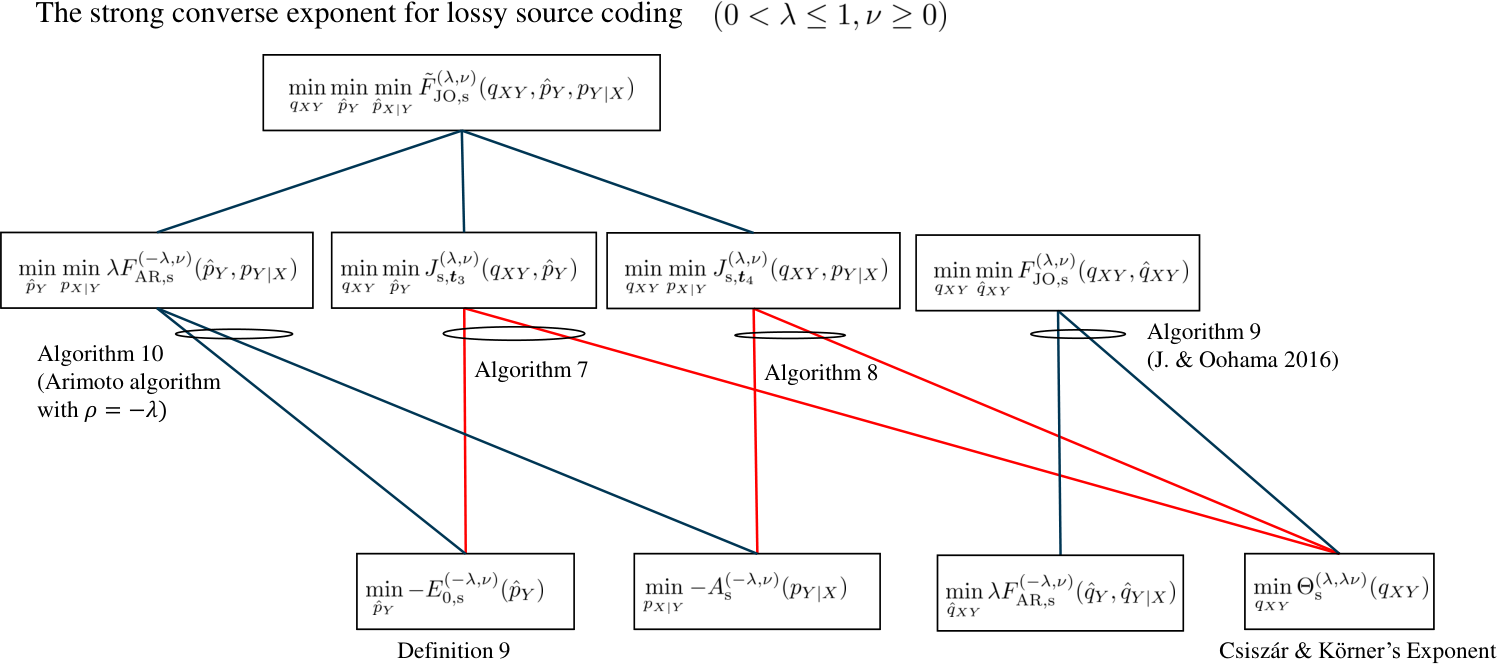
In this paper, we define a new family of algorithms for computing the strong converse exponent for lossy source coding, based on the idea similar to the algorithm family of Tridenski et al. This new algorithm family includes our previous algorithm [25] as a special case. We then discuss two other special cases, which are called Algorithms 7 and 8. The relation between these three cases of the new algorithm family and the Arimoto’s algorithm is shown in Fig. 2. The structure of the relationship between these algorithms corresponds perfectly to Fig. 1. The new algorithm family uses a parameterized objective function which includes the objective functions shown in the three right boxes in the upper row in Fig. 2. We introduce in Definition 9 a new expression of the strong converse exponent that is similar to Blahut exponent, except that the range of the slope parameter is . The rightmost in the bottom row is an optimization problem expressing Csiszár and Körner’s strong converse exponent. The exponent that we introduce in Definition 9 is the leftmost in the bottom row in Fig. 2. In Algorithm 7, the objective function in Blahut’s exponent, but with a negative , and that of Csiszár and Körner’s exponent appear alternately. The convergence of the algorithm proves that for all rate , the exponent of Definition 9 coincides with Csiszár and Körner’s exponent. This paper also shows in Theorem 5 that Arimoto algorithm originally proposed for positive works correctly for the parameter as well.

This paper is organized as follows: Section II defines symbols and notations used in this paper and reviews the error and the strong converse exponents in channel coding and source coding. We discuss channel coding in Sections III and IV and source coding in Sections V and VI. Algorithms for computing the strong converse exponent in channel coding is discussed in Section III. New iterative algorithms are defined and the convergence of the algorithms to an optimal distribution is proved. We then compare the proposed algorithm with Arimoto’s algorithm, Tridenski and Zamir’s algorithm, and our previously proposed algorithm. In Section IV, we give a new proof for the fact that Csiszár and Körner’s error exponent matches with Gallager’s exponent. In Section V, computation algorithms for the strong converse exponent in lossy source coding are proposed. In Section VI, we prove that Arimoto’s algorithm for computing error exponent of lossy source coding is applicable for computation of strong converse exponent. We also show that Arıkan and Merhav’s guessing exponent [26] can also be computed by Arimoto’s algorithm for lossy source coding.
II Definitions of exponent functions
As a preliminary to state the main result, this section reviews the definition of the error and the strong converse exponent functions in channel coding and lossy source coding listed in Table I. Each of these exponent functions is defined as an optimization problem with respect to a probability distribution.
II-A Exponent functions in channel coding
We consider a DMC with finite input and output alphabet and that is subject to an input cost constraint. Let , , , be the transition probability of the DMC. Let be a cost function for sending and the average cost of sending codeword is . Let be a coding rate and be a maximum allowable cost. We define four functions.
Definition 1
For and , Gallager’s random coding error exponent is defined by
| (1) |
where is a set of probability distributions on the input alphabet and
| (2) |
is called Gallager’s function for cost constraint channels. We use the natural logarithm.
Definition 2
For and , Arimoto’s strong converse exponent is defined by
| (3) |
Definition 3
Csiszár and Körner’s error exponent is defined by
| (4) |
where is a set of conditional probability distributions of given , is the conditional relative entropy defined by
and is the mutual information. We follow the convention that , and for .
Definition 4
Dueck and Körner’s strong converse exponent is defined as
| (5) |
where is a set of probability distributions on .
Tridenski and Zamir gave a new expression of the optimal strong converse exponent [27, Eq.(32)]. The following expression is an extension of Tridenski and Zamir’s exponent to DMCs under cost constraint.
Definition 5
Tridenski and Zamir’s strong converse exponent is defined by
| (6) |
where and are joint distributions defined by and .
II-B Exponent functions in Lossy source coding
Consider a DMS with source alphabet and probability distribution . Let be a reproduction alphabet and be a distortion measure. We consider the case that the distortion with a block length is measured by . Let be the coding rate and is the maximum allowable distortion. We assume that both and are finite sets and allow to be different form and that for every there exist at least one satisfying . We define three exponent functions.
Definition 6
Blahut’s error exponent [20] is defined by
| (7) |
The error exponent of the lossy coding problem was established by Marton [21].
Definition 7
Marton’s error exponent for lossy source coding was defined by
| (9) |
where
is a rate distortion function. Marton proved that exponents of upper and lower bounds of the error probability for an optimal pair of encoder and decoder are both given by . That is, Marton’s exponent is optimal.
The exponential strong converse theorem for lossy source coding was established by Csiszár and Körner [22].
Definition 8
Csiszár and Körner’s strong converse exponent for lossy source coding is defined by
| (10) |
was proven to be optimal [22]. The strong converse exponent for lossy source coding in Blahut style has not been known. We define
Definition 9
For and , we define
| (11) |
We will show in Section VI-A that coincides with .
Marton mentioned in [21, Section III] that the continuity of with respect to had not been established. Note that the rate distortion function is not convex in for a fixed . Therefore, for a fixed , the feasible set in (9) is not convex. This implies that may jump at some . Then, in 1990, Ahlswede gave an example that Marton’s exponent is not continuous in , using a distortion measure with a special structure [29]. This implies Eq.(9) is a non-convex optimization problem and Blahut’s and Marton’s exponents do not match in general. The difficulty lies in that we can select any distortion measure on . We normally expect is a function similar to the distance between and and, fortunately, it is guaranteed that if belongs to an important class of distortion measure that can be expressed as a function that only depends on the difference of and , then is a convex function of [26], which immediately implies that . Hamming distortion is included in this class. See also [30] and [22, Exercise 9.5].
Hereafter, when it is obvious from the context, we omit the symbol for the set of probability distribution such as and and write only the probability distribution under and symbols.
III Algorithms for the channel-coding strong converse exponent
The algorithms for computing the channel coding strong converse exponent are discussed in this section. Arimoto’s algorithm [12] was the first for computing the strong converse exponent, which is based on Arimoto’s expression (3). Usually we are interested not only in the value of the exponent function, i.e. the maximum or the minimum value of the objective function, but also in the probability distribution that attains the optimal value. The optimal distribution is not necessarily unique. In Arimoto’s algorithm as well as other algorithms described in this paper, the probability distribution converges to one of the optimal distributions when the optimal distribution is not unique.
About 40 years later, the authors [14] proposed a new algorithm for computing the strong converse exponent based on Dueck and Körner’s expression (5). Subsequently, Tridenski and Zamir [16] proposed another algorithm that was based on their strong converse exponent expression (6). Then, Tridenski et al. [13] proposed a family of algorithms which includes [14] and [16] as special cases.
The main purpose of this section is to illustrate the overall picture of Fig. 1. We begin with the algorithm family of Tridenski et al. [13] and then consider important special cases. Section III-B explains Tridenski and Zamir’s algorithm. We will show the outstanding property of this algorithm that the objective function takes alternately the forms of the objective functions appeared in Arimoto’s and Dueck and Körner’s exponent. Thus, the convergence of the algorithms to the global minimum directly implies the match of the two exponents. This paper is the first to point out such a desirable property of Tridenski and Zamir’s exponent. Then, in Section III-C, we describe the properties of another special case denoted by Algorithm 3. The importance of this special case is clarified for the first time in this paper. The surrogate objective function used for Algorithm 3 plays an important role for the error exponent, too. This topic is described in Section IV. We then compare Tridenski and Zamir’s algorithm and Algorithm 3 with Arimoto’s and our previously proposed algorithm.
Before proceeding to Section III-B, we review the basic properties of Dueck and Körner’s exponent, which are commonly utilized in all the algorithms in Fig. 1 except for Arimoto’s algorithm. Put . Let be the channel capacity under input constraint . Dueack and Körner’s exponent satisfies the following property.
Property 1
- (a)
For a fixed , is monotone non-decreasing function of . For a fixed , is monotone non-increasing function of .
- (b)
is a convex function of .
- (c)
For , and for , is strictly positive.
Proof: See [31] for the proof.
Then, we give a parametric expression of the exponent function. To this aim, we define the following functions:
Definition 10
For any fixed , we define
| (12) |
Definition 11
For fixed and , we define
| (13) | ||||
| (14) |
It was shown [15, Appendix C] that, for a fixed and , the function is convex in . The following lemma states that the Dueck and Körner’s exponent is obtained by evaluating the minimum of .
Lemma 1 ([15])
For any fiex , , and , we have
| (15) |
For any , and , we have
| (16) | ||||
| (17) |
Computation of the exponent functions involves the Legendre-Fenchel transformation (LFT) [32]. The LFT of a function of an -dimensional vector is defined by
| (18) |
where is the transpose of . We use the LFT to derive a parametric expression of the exponent functions, by considering supporting lines to the curve of exponent functions. This is the same as the computation of the rate distortion function and the channel capacity under cost-constraint, which is obtained by considering the supporting lines of the rate-distortion function and the capacity-cost function [22, Chapter 8].
By comparing Eq.(15) with (18), we see that for fixed , as a function of is the one-dimensional LFT of as a function of . Then, by comparing Eq.(16) with (18), we see that for a fixed , is the one-dimensional LFT of as a function of . This implies that is computed by the two-dimensional LFT of as a function of . The numerical computation of the LFT can be performed efficiently. See, for example, [33]. Thus, the target for the algorithm is to compute an optimal that attains for any given and . Fig. 3 shows a rough sketch of the error and the strong converse exponents in channel coding. In Fig. 3, for a fixed , as a function of is depicted by a solid curve, and its supporting line of slope , expressed by , is depicted by dotted line. The -axis intercept of this line is called the generalized cutoff rate [34], denoted by in this figure. If , , while if , , where . See [15, Lemma 10] for detail.

For given , and , we do not have general formula for the explicit expression of the optimal joint distribution that attains (14). For and , one can easily see that holds and is evaluated as follows:
| (19) |
where (a) holds with equality if and only if for such that for all and (b) holds with equality if and only if .
We now perform a change of variables: let , and instead of the parameter pair , let be the variable parameter pair. By doing so, in the limit of , one of the new algorithms is reduced to the Arimoto-Blahut algorithm that computes the channel capacity under cost constraints.
In the following subsections, we describe algorithms shown in Fig. 1. We begin with the algorithm family of Tridenski et al. III-A. The algorithm family includes Tridenski and Zamir’s algorithm [16] as a special case, which is explained in Section III-B. Then, another special case, Algorithm 3, is explained in Section III-C. Comparison with Arimoto’s and the authors’ algorithms are given in Sections III-D and III-E.
III-A Algorithm family of Tridenski et al.
In [13], Tridenski et al. proposed a family of computation algorithms that includes two previously proposed algorithms as spacial cases33 3 As in the case of [16, 17], there are two types of the algorithm families. One is for a fixed rate and the other is for a fixed slope parameter . The latter is discussed here. . One is our algorithm [15, 14] and the other is Tridenski and Zamir’s algorithm [16]. The objective function for the algorithm family is [13, Eq.(24)]
| (20) |
where is a vector of four non-negative coefficients and
| (21) |
From the definition, we have the following lemma.
Lemma 2
For any fixed , , , and any fixed , is minimized by and its minimum value is
| (22) |
This implies that
| (23) |
Proof: This lemma follows from Eqs. (20) and the condition for . ∎
Vontobel et al. [5] pointed out that to derive an Arimoto-Blahut type algorithm for a given optimization problem, say , it is required to find a surrogate objective function that satisfies the following three conditions:
- a)
The surrogate function takes the same value as at , i.e., .
- b)
is never below , i.e., for all .
- c)
Minimizing over can be done in a computationally efficient way.
Assume a satisfies the three conditions. Then, by the iterative algorithm with a given initial value , the value of the objective function is monotone non-increasing. To prove convergence of the algorithm to its optimal value, a separate proof for each objective function is needed. For the current optimization problem, we replace , , and , respectively with , , , and . It is easily confirmed that the condition a) and b) are satisfied in this case. Regarding the condition c), Tridenski et al. showed the condition on and so that optimal that minimizes for a fixed is expressed explicitly. The condition is expressed by the following lemma [13].
Lemma 3 (Lemma 3 in[13])
Define and
| (24) |
If , then for , the optimal distribution that attains the minimum of for a fixed is expressed explicitly.
The parameterized surrogate objective function produces a parameterized alternative expression of the exponent. To illustrate this, we define a set of representations of the exponent as
| (25) | ||||
| (26) |
We also define
| (27) |
| (28) |
Fig. 4 illustrates the relation between Dueck and Körner’s exponent, , , , , and some special cases. Note that and are the set of expressions of the minimization problems and the values of all elements in and coincide because
holds for any . Then, the large circle at the top of Fig.4 expresses the set . The small circles and are the subsets of for which belongs to and , respectively. The large circle at the bottom of Fig.4 expresses the set , and and are the subsets of . Tridenski and Zamir’s algorithm [16], described in Section III-B, corresponds to the case and the authors’ previous algorithm [15, 14], described in Section III-E, corresponds to the case . The expression belongs to , belongs to , and belongs to the intersection of and . Each element in has two arrows. The arrow heading straight down means that is obtained by executing the minimization with respect to , whereas the arrow heading right down means that is obtained by executing the minimization with respect to .

| (29) |
| (30) |
Algorithm 1 shows the Tridenski et al.’s algorithm family44 4 They appear to have typographic errors in [13, Lemma 3]. The parameters , , and were misspelled as , , and , respectively.. Then, the convergence of the probability distribution was stated in [13, Theorem 2] as
See [13] for the proof.
The above theorem states that converges to the optimal distribution that minimizes . Does this optimal distribution is the same as the one that minimizes ? The following proposition provides the answer to this question.
Proposition 1
For any , , and , we have
| (32) |
Proof:
The first inequality follows from the definition of and the non-negativity of the divergence and the second inequality follows from (27). ∎From this proposition, is guaranteed to converges to the optimal distribution that minimizes .
Here we give three remarks on Algorithm 1. The first one is that the probability update rules for and were parameterized with two parameters by letting , , and in[13]. The reduction of the number of parameters is possible because we have and therefore , and are redundant. Hence, the function of is the same as that of and that of is the same as that of . The second is that by selecting the initial distribution so that every element is non-negative, we can avoid the situation that for some and that for some . A possible choice for is the uniform distribution. The last remark is that The left hand sides of Eqs.(29) and (30) are joint distributions but they can be separated and respectively. The following lemma will be used in the following subsections.
Lemma 4
Assume , , and are fixed. If , then is minimized by
| (33) | ||||
| (34) |
where
| (35) |
The minimum value is
| (36) |
If , then is minimized by
| (37) | ||||
| (38) |
where
| (39) |
The minimum value is
| (40) |
The procedure of the derivation is the same as the proof of Theorem 1 and the proof is omitted here.
From this lemma, we have the following corollary, which shows the relation between and Arimoto’s exponent. This paper is the first to point out such an important relationship.
Corollary 1
For , any fixed , , and any fixed , is minimized by
| (41) | ||||
| (42) |
Denote the joint distribution computed from the above and by . The minimum value of for a fixed is
| (43) |
This implies that
| (44) |
This corollary will be used in the next subsection. We also give the following corollary, which will be used Section III-C. In order to describe the corollary, we use the following function that appears in Arimoto’s algorithm [12].
Definition 12
For a given transition probability and , , we define
| (45) |
Corollary 2
For , any fixed , , and any fixed , is minimized by
| (46) | ||||
| (47) |
Denote the joint distribution calculated from the above and by . Then, the minimum value of for fixed is
| (48) |
This implies that
| (49) |
It is important to note that the algorithm family includes the algorithm of Tridenski and Zamir [16] and the algorithms previously presented by the authors [14, 15] as special cases, allowing multiple algorithms to be discussed from a unified point of view. On the other hand, it is more prospective to focus on individual algorithms in order to describe their relationship to the Arimoto algorithm. In the following subsections, the three special cases are described in detail.
III-B Algorithm 2
We call Tridenski and Zamir’s algorithm [16] as Algorithm 2. They proposed two types of algorithms. One is the algorithm for computing Tridenski and Zamir’s exponent (6) for fixed without using the slope parameter [17, 16] and the other is for fixed slope[16, Section VII]. This subsection describes the latter. Although this algorithm is a special case of the algorithm family (Algorithm 1), it has attractive properties and therefore we will discuss this algorithm separately.
For describing Tridenski and Zamir’s algorithm, we need to show that coincides with . Tridenski and Zamir introduced the following function[16, Section VII]:
| (50) |
The following lemma holds.
Lemma 5
For fixed and , is minimized by and its minimum value is
| (51) |
Proof: By the definition of the ordinary and the conditional divergences, we have
| (52) |
Because is non-negative and takes zero if and only if , we have , which completes the proof. ∎
Then we have the following lemma.
Lemma 6
For any and , we have
| (53) |
In [27, 16], the proof of the the match of and for a DMC without input-cost was given. Because the match of and is a known fact [35], this suggests , too. However, it should be better if we can show this match directly.
Proof: We have the following chain of equalities:
| (54) |
Step (a) and (d) follows from the identity . Step (b) follows from the mini-max theorem because the expression in the parenthesis is convex in and linear in for a fixed . Step (c) follows from Lemma 5. ∎
Now, we describe Tridenski and Zamir’s algorithm for fixed slope parameter . This algorithm corresponds to the case of . The objective function of Tridenski and Zamir’s algorithm is therefore
| (55) |
Trindenski and Zamir’s algorithm is based on the double minimization of with respect to and . From Lemma 5 and the definition of , for any and , we have
| (56) |
Tridenski and Zamir’s original algorithm in [16] is the algorithm for the channel without cost constraint. Eq.(56) shows that the function is the extension of to channels under input cost.
The function satisfies the following property.
Property 2
For any fixed , and any fixed , is convex in . For any fixed , and any fixed , is convex in .
See Appendix A for the proof.
Tridenskii and Zamir’s algorithm shown in Algorithm 2 in obtained by setting in Lemma 4. The probability update rule follows from Corollary 1. Here, Eq.(59) is a computation of the marginal distribution from .
| (57) | ||||
| (58) | ||||
| (59) |
Because Algorithm 2 is a member of the algorithm family, the convergence theorem of this algorithm is supported by Theorem 1.
Now, we can state the following attractive property of Tridenski and Zamir’s algorthim:
Proposition 2
For , we have
Proof: Step (a) follows from Lemma 2 and step (b) follows from Corollary 1. Step (c) follows from (23) in Lemma 2 and (44) in Corollary 1. This completes the proof. ∎
A feature of Algorithm 2 indicated by Proposition 2 is that the -function for Arimoto’s strong converse exponent and the for the Csiszár and Körner’s exponent appear alternately. The convergence of Algorithm 2 immediately gives the proof of the fact that Dueck and Körner’s and Arimoto’s exponents coincide, stated in the following proposition.
Proposition 3 ([24])
Suppose the channel transition probability is given. Then, for any , , we have
| (60) |
Proof:
We have the following chain of equalities:
| (61) |
Step (a) follows from definition 3, Step (b) follows from the equation (c) in Proposition 2, Step (c) holds because we have for a fixed , and Step (d) follows from Definition 5. ∎
The match of Dueck and Körner’s and Arimoto’s strong converse exponents is well-known but no proof was written in [24]. An explicit proof for the channel with cost constraint is found in [35]. In the above proof, the convergence of Tridenski and Zamir’s algorithm plays a critical role. This proof is interesting because it differs significantly from previously known proofs.
In Section III-D, we will compare Tridenski and Zamir’s algorithm with Arimoto’s algorthm, where update rule (57) is the same as in Arimoto algorithm. Another update rule (58) is not explicitly used in the Arimoto algorithm, but we will give the view that (58) is a hidden update rule of the Arimoto algorithm.
III-C Algorithm 3
In this subsection, we consider another special case, . This case has not been discussed in depth, but is important in the sense that during the alternate updates of the probability distribution, the corresponding algorithm alternates between the form of the Dueck and Körner’s exponents and the form of the alternative representation of the Arimoto’s strong converse exponent. By extending the domain of from to , we will derive an important property for the two types of expressions of the error exponent, which is the topic of Section IV. Because with negative is not included in , the property of in this case is described in this chapter.
We use the following objective function of and :
| (62) |
The reason why the conditional distribution is denoted as instead of in (62) is to unify the notation of probability distributions in Fig.1. The first thing to check is the convexity of this function. Here, we check it for . Positive is for strong converse exponent and negative is for error exponent.
Property 3
- a)
For any fixed (resp. ), , and any fixed , is convex (resp. concave) in .
- b)
For any fixed (resp. ), , any fixed , and any fixed , is convex (resp. concave) in .
- c)
For any fixed , , any fixed and , is convex in .
See Appendix A for the proof.
An algorithm for computing the strong converse exponent based on Lemma 2 and Lemma 4 with is shown in Algorithm 3. Eq.(65) is simply a conditional probability of backward channel computed from .
| (63) | ||||
| (64) | ||||
| (65) |
Similarly to the Proposition 2, the following proposition holds:
Proposition 4
For , we have
Proof: Step (a) follows from Lemma 2 and step (b) follows from Corollary 2. Step (c) follows from (23) in Lemma 2 and (49) in Corollary 2. This completes the proof. ∎
Proposition 4 shows that the objective function takes the forms of the alternative expression of Arimoto’s exponent and the parametric expression of Dueck and Körner’s exponent alternately and that monotonically decreases. Next theorem shows that converges to .
Theorem 2
See Appendix B for the proof.
We give a remark that when , Algorithm 2 reduces to and when Algorithm 3 reduces to . In these cases, the probability distributions are not updated. Therefore, we cannot use Algorithm 2 and Algorithm 3 respectively when and . However, these algorithms work in the opposite cases. In the limit of , (64) becomes
and Algorithm 3 reduces to the Arimoto-Blahut algorithm for computing the channel capacity.
III-D Comparison with Arimoto algorithm for channel coding exponents
This subsection gives comparisons between Tridenski and Zamir’s algorithm, Algorithm 3, and Arimoto’s algorithms for channel coding [12]. Arimoto’s algorithm was derived from the optimization problem appeared in (1) and (3). Unlike Tridenski and Zamir’s algorithm and Algorithm 3, Arimoto’s algorithm can be applied to the computation of both the error and the strong converse exponents.
For fixed and , the function is concave in when is positive and is convex in when is negative. Arimoto chose as an objective function which is concave for positive and negative . Arimoto [12] introduced the following function.
Definition 13
For a given transition probability of a channel , , and , we define
| (66) |
Arimoto’s algorithm is an algorithm that finds
| (67) |
by optimizing and alternately. Arimoto proved the following theorem.
Theorem 3 (Arimoto[12])
For a fixed , and any fixed , we have
| (68) |
and the maximum value is attained by
| (69) |
On the other hand, for a fixed , and any fixed , we have
| (70) |
The maximum value is attained by
| (71) |
See [12] for the proof. A quick proof will be shown later. Based on Theorem 3, Arimoto presented an iterative algorithm shown in Algorithm 4.
| (72) | ||||
| (73) |
When , Algorithm 4 reduces to the ordinary Arimoto-Blahut algorithm for computing the channel capacity. For the case of , is interpreted as its limiting function, i.e.,
| (74) |
When , is interpreted as
| (75) |
The rhs of Eq.(75) is the function that appears in Arimoto-Blahut algorithm for finding the channel capacity. Thus we can regard as a generalization of (75) to the case .
Corollary 3
For any fixed and , we have
| (76) |
Corollary 4
Define the following functions.
| (77) | ||||
| (78) |
Then, we have
| (79) |
We call and alternative representations of the error exponent and the strong converse exponent.
At the end of this subsection, we give a proof of Theorem 3 using the conditional Rényi divergence. Many attractive properties of Rényi entropy, Rényi divergence, and exponent function were described by Verdú [36, 37] and Cai and Verdú [38]. One of the important properties discussed in [36, 37, 38] is that the Gallagar’s error exponent is expressed by using Arimoto’s conditional Rényi entropy [39] as well as Sibson’s mutual information of . The Rényi divergence and the conditional Rényi divergence of order are defined by
| (80) | ||||
| (81) |
Rényi divergence and conditional Rényi divergence are non-negative and vanish if and only if and , respectively. To the best of our knowledge, the following relations have not been pointed out so far.
Lemma 7
For a given , , and , set
| (82) | ||||
| (83) | ||||
| (84) |
Then we have
| (85) | ||||
| (86) |
See Appendix C for the proof.
Proof of Theorem 3: Eqs.(68) and (70) are proved by the nonnegativity of Rényi divergence and the conditional Rényi divergence. The conditions for Rényi divergence and the conditional Rényi divergence to take zero directly prove (69) and (71). This complets the proof. ∎
It should be noted that although Eq.(57) in Algorithm 2 and Eq.(64) in Algorithm 3 were derived from Dueck and Körner’s exponent function, their functional structures are the same as Eqs. (72) and (73) in Arimoto’s algorithm. Note also that the structure of (83) in Lemma 7 is the same as (58). In Arimoto algorithm, is not used. However, this probability distribution appears when we express the difference between and by Rényi Divergence as in (85). We will see the same form as (83) in the next section again.
III-E Comparison with our previous algorithm
This subsection gives a comparison between Tridenski and Zamir’s algorithm, Algorithms 3, and our previous algorithm in [14]. Before [14], no algorithm was known for computing the optimal distribution for Dueck and Körner’s strong converse exponent. The algorithm for DMCs without input cost constraint was extended to the algorithm for DMCs under input cost [15]. We introduced the following function to obtain the minimum of .
| (87) |
Regarding this function, the following two lemmas hold.
Lemma 8 ([15])
For a fixed , and , is minimized by and its minimum value is
| (88) |
This implies that
| (89) |
Lemma 9 ([15])
For a fixed , and , is minimized by
| (90) |
and its minimum value is
| (91) |
This implies that
| (92) |
The algorithm for computing is shown in Algorithm 5. In [15], the condition for the termination of the iterative updating is mentioned but is omitted here.
| (93) |
The important observation here is that the function in the rhs of (91) is exactly the same as the function in the rhs of Eq. (66). Then, it can be seen that the function in (87) satisfies
| (94) |
From this equation, we observe that is equal to , where . Here, and are the marginal and the conditional distribution derived from the joint distribution . However, what if we can replace with another conditional distribution function that is not related to ? By slightly modifying , we have introduced the following function ( is also replaced with ) [15].
| (95) |
Then, we can easily prove the following lemmas.
Lemma 10 ([15])
For a fixed , and , we have
| (96) |
The minimum is attained if and only if and holds.
Lemma 11 ([15])
For a fixed , , , and , we have
| (97) |
The minimum is attained if and only if
| (98) |
Proposition 5
For a fixed , , and , we have
| (99) |
This proposition clearly shows that the Dueck and Körner’s exponent is equal to the double minimization form of Arimoto’s alglrithm. It is an important property of the function that the double minimization form is derived from this function. Moreover, we immediately obtain the following two lemmas:
Lemma 12
For fixed , , , and , we have
| (100) |
Lemma 13
For a fixed , , and , we have
| (101) |
Fig.5 shows the relationship between the triple minimization , the double minimization form of Arimoto’s algorithm, , and . This figure shows that the three double minimization forms are obtained by evaluating the minimum value with respect to one probability distribution for the triple minimization form and removing one minimization operation.

Because the objective function is a special case of the parameterized surrogate objective function , we can construct a parameterized function such that is a special case of the function. We define such a parameterized function as
| (102) |
This function reduces to when . By introducing this function, the following interesting things can be seen. The function in the double minimization form, on which Arimoto’s algorithm is based, is replaced by a parameterized function , from which a parameterized algorithm is derived. In Arimoto’s algorithm and are alternately updated, while and are alternately updated in the parameterized algorithm. Details of the parameterized algorithm is shown in Appendix D. A special case of is interesting. We expect the parameterized algorithm reduces to Algorithm 4. It actually does so, but it also has extra updating rules for and . It is explicitly written as
| (103) | ||||
| (104) | ||||
| (105) | ||||
| (106) |
Then, the relationship between Algorithms 2, 3, and 4 becomes clearer. Eqs.(103) and (105) are equal to (72) and (73) with . Eqs.(104) and (106) do not appear in Arimoto’s algorithm. However, they appear in (58) and (63) in Algorithms 2 and 3, respectively. The and in (104) and (106) are considered to be natural distribution updating rules, which are derived from the parameterized objective function .
IV The match of Gallager’s and Csiszár and Körner’s error exponents
Arimoto’s algorithm is based on the double maximization expression in Eq.(67) for positive and negative and therefore can be applied for computing both the Gallager’s error exponent and the Arimoto’s strong converse exponent. Algorithms 2, 3, and 5, were derived based on the Dueck and Körner’s expression of the strong converse exponent. Unfortunately, we cannot apply Algorithms 2, 3, and 5 for computing the Csiszár and Körner’s error exponent because of the following reasons. Comparing Eq.(4) with (5), Eq. (5) is a minimum value of a functional with respect to a joint distributions, whereas Eq.(4) is a saddle point of a functional. At the saddle point, the functional is maximized with respect to the input probability distribution and it is minimized with respect to a conditional distribution . In order to derive Arimoto-Blahut type algorithm, we must find an expression that can be defined as a joint maximization problem or a joint minimization problem.
This section shows that we can prove that Csiszár and Körner’s error exponent matches with the alternative expression of error exponent defined in (77). Because the alternative expression matches with Gallager’s error exponent, the proof immediately implies that Csiszár and Körner’s exponent matches with Gallager’s exponent. For the proof, we use the surrogate objective function that was used to derive Algorithm 3. Thus, the result of this section is an application of Algorithm 3. It should be noted that the objective functions that are used in Algorithm 2 and 5 cannot be applied to prove the match of the two error expressions of error exponent.
The following proposition shows that Csiszár and Körner’s exponent matches with Gallager’s exponent.
Proposition 6
For any and , we have
| (107) |
In this section, we first give an overview of the standard method of proving Proposition 6. Then, a new proof is presented.
IV-A A proof shown in Exercise 10.24 in [22]
The following steps are suggested in [22, Exercise 10.24] to prove55 5 To be precise, it shows the proof that the two forms of the sphere-packing exponent function match. Proposition 6 which states that Csiszár and Körner’s exponent and Gallager’s exponent match. In order to explicitly discuss the difference between this steps and our proof, we describe the steps in detail. Cost constraints essentially have no effect on the proof step. Thus, as in [22, Exercise 10.24], we consider a DMC without cost constraint in this subsection. See also Lapidoth and Miliou [40], showing that these two exponents are Lagrange dual each other.
- 1.
Prove the equation
(108) - 2.
Define
(109) and prove the equation
(110) where
(111) - 3.
In the following, we give an upper and a lower bounds on . If the upper and the lower bounds are equal, the bound is found the desired saddle point. First, by the concavity of function and Jensen’s inequality, we have
(112) Then, show that the right hand side of (112) is minimized by
(113) where is a normalization factor. Denote this by .
- 4.
- 5.
Fix to some distribution to give an upper bound of . For this purpose, assume . Then,
(116) Step (a) follows from Eq.(115). Hence, is found to be an upper as well as lower bounds of . Therefore
(117)
As shown above, Step 3 uses Jensen’s inequality and steps 4 and 5 evaluate the upper and lower bounds. In the next subsection, we show another procedure to show the match of the two error exponents. In this new procedure, the evaluation of each step is explicit and thus the new proof is more elementary than the standard proof. The interesting point is that we use the function that was used to derive Algorithm 3.
IV-B New proof for the match of random coding error exponents
Here, we give a new proof for the match of Gallager’s and Csiszár and Körner’s error exponents. In the previous section, we removed the cost constraint for simplicity and to match the description in [22, Exercise 10.24]. In this section, we consider DMCs with cost constraints. The proof steps are the same with or without cost constraints.
Csiszár and Körner’s exponent is expressed using the function but with negative (we put ). When , satisfies the following property.
Property 4
Suppose and are fixed. Then is concave in for a fixed and convex in for a fixed .
Proof: By definition, we have . The first term is concave in for a fixed and is convex in for a fixed . The second term is convex in for a fixed and is a linear function of for a fixed . The last term is linear in . Therefore, the property holds. ∎
We use defined in (62) for with . Define
| (118) |
Property 4 is used to prove the following two lemmas.
Lemma 14
For any fixed and any fixed , is maximized by and the maximum value is
| (119) |
This implies that
| (120) |
Proof: It is obvious from the definition of .
Lemma 15
For any fixed , , and , is minimized by
| (121) |
and the minimum value is
| (122) |
This implies that
| (123) |
Lemma 16
For any fixed and any fixed , is maximized by
| (124) |
and the maximum value is
| (125) |
This implies that
| (126) |
Proof of Proposition 6: For any fixed , , we have
| (127) |
Step (a) follows from Lemma 14, In step (b), the interchange of the order of and is justified because of Property 3. Step (c) follows from Lemma 15 and step (d) follows from Lemma 16. Therefore we have
| (128) |
Step (e) follows from (108), step (f) follows from (127), and step (g) follows from Corollary 4. This completes the proof. ∎

A comparison of the proof in [22, Exercise 10.24] and our proof is shown in Fig. 6. The guideline shown in [22, Exercise 10.24] is a standard method to prove the match of Csiszár and Körner’s exponent and Gallager’s exponent. It is interesting that our procedure uses Corollary 4, i.e., the match of and , which was derived by Arimoto’s algorithm. It should be noted that due to the structural difference with , the function cannot be used to prove the match between the two exponents. The difference is that for , the joint distribution can be separated and as shown above, while it is separated as and for
If we think the double maximization in the third line of (127) will lead to an algorithm, that’s a misunderstanding. In fact, if the optimum solution when one of the variables is fixed cannot be written explicitly, it will not lead to a computation algorithm for alternating optimization like the Arimoto algorithm. The reason why it is difficult to derive the computation algorithm for the Csiszár and Körner’s error exponent is that the the exponent is defined as the minimax problem, unlike the Dueck and Körner’s strong converse exponent. Even if the form of the double maximization problem can be derived, it is still necessary to be able to explicitly write the solution when one of the variables is fixed. This condition makes it difficult to derive the computation algorithm for Csiszár and Körner’s error exponent.
V Algorithms for the lossy source-coding strong converse exponent
So far, we have discussed computation algorithms for the correct and error decoding probability exponents in channel coding. This section describes algorithms for computing exponents in lossy source coding. The first algorithm for computing Csiszár and Körner’s strong converse exponent was due to the authors [25]. In the following subsection, we propose a family of algorithms for computing the strong converse exponent in lossy source coding that is similar to the algorithm family of Tridenski et al. The previously proposed algorithm is included in the new algorithm family. Then, two special members of the algorithm family that have important properties are described in detail. Fig. 7 shows the relation between the algorithms. The structure of the diagram of Fig. 7 is quite similar to Fig. 5. In Fig. 7, nine expressions defined by minimization problems are shown. They are the quantities used to express the strong converse exponent with parameter and . The function will be defined in Section V-D.
In Arimoto’s paper [12], an algorithm for computing Blahut’s error exponent was given. The validity of computing the strong converse exponent with Arimoto algorithm has not been clarified. The issue is discussed in this section and Section VI-A and its validity is clarified.
The rate-distortion function is generally not convex in and therefore it is difficult to develop an algorithm directly from the expression of (5). This motivated us to define the following function:
Definition 14
For any fixed , , we have
| (129) |
Then, we have the following lemma:
Lemma 17
For any fixed , , and any fixed , we have
| (130) |
Lemma 17 assures that can be computed by evaluating , the form of which is quite similar to . In the representation of , we could eliminate the rate-distortion function. Based on this representation, we can derive an algorithm.
The function satisfies the following property, which is required to derive its parametric expression:
Property 5
- a)
is a monotone non-increasing function of for a fixed and is a monotone non-increasing function of for a fixed .
- b)
is a convex function of .
- c)
takes positive value for . For , .
- d)
For , we have
See Appendix G for the proof.
Then, we define the following function that will be used as an objective function of the algorithm.
Definition 15
For any fixed , we define
| (131) |
Definition 16
For any fixed , , and , we define
| (132) | ||||
| (133) |
The subscript ‘’ means that this function is the source coding counterpart of the corresponding function in channel coding. One can observe that Eq.(132) for is similar to Eq.(13) for for the channel coding.
Lemma 18
For any fixed , , and , we have
| (134) |
For any fixed , , and , we have
| (135) | ||||
| (136) |

Eq.(134) shows that is computed by the Legendre transform of with respect to . Then, Eq.(135) shows that is computed by the Legendre transform of with respect to . This immediately implies that is computed by the two-dimensional Legendre transform of whose domain is , as shown in Eq.(136). An image of the shape of function is shown in Fig. 8. The supporting line to this function of slope is expressed by . We can easily see that by choosing and for every and with . For , we have
| (137) |
The generalized cutoff rate, denoted by is the -axis intercept of this supporting line. Therefore
We now perform a change of variables: let , and instead of the parameter pair , let be the variable parameter pair. By doing so, in the limit of , one of the new algorithms is reduced to the Arimoto-Blahut algorithm that computes the rate distortion function. From (134), we have
| (138) |
In the following subsections, we describe algorithms shown in Fig. 7. The following discussions for source coding are parallel with the discussions for channel coding. In Section V-A, we define a generalization algorithm for lossy source coding inspired by the algorithm family of Tridenski et al.
V-A The algorithm family for lossy source coding
We define the objective function for the family of algorithms for source coding as
| (139) |
where and . The second term of the above equation is exactly the same as that of (20). We have the following lemma:
Lemma 19
For fixed , , and , is minimized by and the minimum value is
| (140) |
This implies that
| (141) |
holds for any .
Proof:
We have because of the non-negativity of the divergences and conditional divergences. Equality holds if . This completes the proof. ∎
Lemma 20
For fixed , , and , is minimized by and the minimum value is
| (142) |
This implies that
| (143) |
In Lemma 20, optimal is expressed implicitly. Explicit form for the optimal is needed to use as a surrogate function for . It is easy to verify that function (139) satisfies a) and b) among the three conditions listed in Section III-A for any . Regarding the condition c), we have the following lemma.
Lemma 21
Define
| (144) | ||||
| (145) |
If , then for , the optimal distribution that attains the minimum of for a fixed is expressed explicitly.
The proof of Lemma 21 is provided in Appendix I. The algorithm family derived from is given in Algorithm 6.
| (146) | ||||
| (147) | ||||
| (148) |
| (149) | ||||
| (150) | ||||
| (151) |
| (152) |
Fig. 9 illustrates the relation between the expression of Csiszár and Körner’s exponent, the double minimization form of the surrogate objective function with parameter , and the expressions derived from the parameterized objective function by fixing and optimizing the objective function with respect to . Define
| (153) |
Define four sets of minimization problems as follows:
| (154) | ||||
| (155) |
for . Replace the in (154) and (155) with to define the sets and . Then, the large circle at the top of Fig. 9 expresses the set . The two small circles within express and . The expression that appeared in (11) is included in and the expression that will appear in Section V-C is included in . The expression which will appear in Section V-D is included in the intersection of and .
Proposition 7
For , we have
Proof:
Step (a) follows from Lemma 19 and step (b) follows from Lemma 20. Step (c) follows from (141) in Lemma 19 and (143) in Lemma 20. This completes the proof. ∎
The convergence of the algorithm is stated as follows:
Theorem 4
For any , , , and , the series of distributions defined by Lemma 6 converges to an optimal distribution that minimizes .
See Appendix J for the proof.

In the following two subsections, two special cases of the algorithm family are discussed. The two cases are and . The algorithm of the first case is called Algorithm 7. Using Algorithm 7, we can show that Csiszár and Körner’s strong converse exponent coincides with a function that is quite similar to Blahut’s error exponent but the slope parameter takes negative value. The objective function of these case are
| (156) | ||||
| (157) |
In Section V-B, we give Algorithm 7 that is derived from and in Section V-C, we give Algorithm 8 that is derived from .
V-B Algorithm 7
In this subsection we describe Algorithm 7. This algorithm is a member of the algorithm family defined in the previous section and has an important application. In Section II-B, we defined a new representation of the strong converse exponent, that is basically the same as Blahut exponent but the parameter takes negative values. The coincidence of this new exponent function with Csiszár and Körner’s exponent is proved by the convergence of Algorithm 7. This is one of the main contribution of this paper and is analogous to the proof of the match of Arimoto’s exponent and Dueck and Körner’s exponent by the convergence of Algorithm 2.
The function satisfies the following two lemmas.
Lemma 22
For any fixed , , and any fixed , is minimized by and the minimum value is
| (158) |
This implies that
| (159) |
Lemma 23
For any fixed , , and any fixed , is minimized by
| (160) | ||||
| (161) |
Denote the joint distribution calculated from the above and by . Then, the minimum value of for fixed is
| (162) |
This implies that
| (163) |
See Appendix E for the proof.
| (164) | ||||
| (165) | ||||
| (166) |
We have the following proposition:
Proposition 8
For , we have
Proof: Step (a) follows from Lemma 24 and step (b) follows from Lemma 25. Step (c) follows from (175) in Lemma 24 and (179) in Lemma 25. This completes the proof. ∎
This proposition shows that in Algorithm 7, the objective function for Blahut’s exponent with and the objective function for Csiszár and Körner’s exponent appear alternately.
Because the Algorithm 7 is a member of the family of the algorithms (Algorithm 6), the convergence of defined by (164)-(166) to the optimal distribution that minimizes is guaranteed by Theorem 4.
We have the following proposition that can be used as a termination criterion by verifying that the is sufficiently close to the optimal distribution.
Proposition 9
A necessary and sufficient condition for to minimize is that
| (167) |
Proof: This is exactly the KKT condition for . Its derivation is straightforward and thus is omitted.
As shown in Proposition 8, equals to the minimum value of over . Using the latter expression, we can show that Csiszár and Körner’s strong converse exponent is equal to (11) which is similar to Blahut’s error exponent, except that it has a negative . We have the following Theorem.
Theorem 5
For any , and , we have
| (168) |
Proof: We have the following equations.
| (169) | ||||
| (170) |
Step (a) follows from Lemma 17, Step (b) follows from Lemma 18, Step (c) follows from the equation (c) in Proposition 8 setting and we put in Step (d). ∎
Theorem 5 says that Csiszár and Körner’s strong converse exponent matches with , which is written in a form similar to Blahut’s error exponent.
At the last of this subsection, we give a remark that the generalized cutoff rate is expressed by the following form.
Property 6
For a fixed and a fixed , let be an optimal that attains the rhs of (138) and let be an optimal distribution that attains . Then we have
| (171) |
V-C Algorithm 8
In this subsection, we discuss another special case of the algorithm family, which uses as a surrogate objective function. The following function that appears in Arimoto’s algorithm will plays an important role in this special case.
Definition 17
For a given source distribution , transition probability of a test channel , and parameters and , define
| (173) |
Lemma 24
For any fixed and , is minimized if and only if and the minimum value is
| (174) |
This implies
| (175) |
Proof: It is obvious from the nonnegativity of the relative entropy .
Lemma 25
For any fixed and , is minimized by
| (176) | ||||
| (177) |
Denote the joint distribution computed from the above and by . The minimum value of is
| (178) |
This implies that
| (179) |
See Appendix E for the proof.
Note that the rhs of Eq.(178) has the same form of the rhs of Eq. (173). We have the following equation.
| (180) |
For a fixed , we can show that the following proposition holds.
Proposition 10
We have
| (181) |
See Appendix K for the proof. Thus, the function , which we call an alternative form, has a natural connection to information theoretic quantities.
An algorithm derived from Lemmas 24 and 25 is shown in Algorithm 8. Algorithm 8 is a member of the algorithm family and therefore its convergence to the optimal distribution is guaranteed by Theorem4.
| (182) | ||||
| (183) | ||||
| (184) |
The following proposition illustrates an important property of Algorithm 11, that and the objective function of Csiszár and Körner’s exponent appear alternately.
Proposition 11
For , we have
V-D Comparison with our previous algorithm
The first algorithm for computing the strong converse exponent for the lossy source coding was given by the authors in [25]. This algorithm is also a member of the algorithm family (Algorithm 6). In this subsection, we describe this special case. Proofs for the theorems and lemmas omitted in [25] are provided in Appendix of this paper.
In [25], we defined the following function.
| (185) |
The following equation holds for this function.
| (186) |
Therefore, corresponds to the case of .
We have the following Lemmas.
Lemma 26
For any fixed , , and any fixed , , is minimized if and only if and its minimum value is
| (187) |
This implies that
Lemma 27
For any fixed , , , and any fixed , is minimized if and only if
and its minimum value is
| (188) |
This implies that
See Appendix G for the proof.
| (189) |
Algorithm 9 for is analogous to Algorithm 5 for . As is discussed below, this observation motivated the development of Algorithms 7 and 8, which are similar to Algorithms 2 and 3.
Similar to Eq.(95) in Section III-E, we replace in the right hand side of (186) with to define
| (190) |
Here, we use the following function introduced by Arimoto [12] to derive his algorithm.
Definition 18
For a given source probability distribution , an output distribution of the test channel , and parameters and , define66 6 More precisely, Arimoto defined (191) multiplied as the objective function and its maximization was discussed.
| (191) |
Then, we have the following lemma.
Lemma 28
For a fixed and , we have
| (192) |
Proof: It is obvious from the definition of and non-negativity of the relative entropy.
Lemma 29
For a fixed , , , and , we have
| (193) |
See Appendix L for the proof.
The above-mentioned relationship is illustrated in Fig. 7. The triple minimization is shown in the top level and is connected to three double minimization, as described in the following proposition.
Proposition 12
For any fixed , , and , we have
| (194) | ||||
| (195) | ||||
| (196) |
We have derived Algorithms 7 and 8 from the double minimization of (194) and (195). The property of the double minimization of (196) will be discussed in Section VI-A. We will show that the algorithm derived from (196) is the same as Arimoto algorithm except that is negative. We then show that Arimoto algorithm works correctly also for negative .
VI Computation of the error exponents in lossy source coding
In this section, Arimoto’s algorithm for computing the error exponents in lossy source coding is discussed and is compared with Algorithms 7, 8, and 9. As shown in Section V-B, Csiszár and Körner’s strong converse is equal to a function similar to Blahut’s error exponent, except that the slope parameter takes negative values. Hence, it is natural to expect that the Arimoto algorithm can be used to compute the strong converse exponent in lossy source coding. To the best our knowledge, this issue has not been published. In Section VI-A, we have proved that Csiszár and Körner’s strong converse exponent matches with a Blahut-style exponent function with parameter . Thus, the answer to the natural question above is yes. Note that the strong converse exponent of lossy source coding [22] was established after the publication of [12], and Arimoto was unable to mention the computation of this exponent.
We will also show that Arimoto’s algorithm can be used to compute Arıkan and Merhav’s guessing exponent [26].
VI-A Arimoto algorithm for lossy source coding exponents
The target of Arimoto’s algorithm for lossy source coding is Blahut’s error exponent for lossy source coding, defined by
| (197) |
The exponent functions satisfy the following property.
Property 7 (Theorem 21 and Theorem 22 in [20])
- (a)
For a fixed , is monotone non-decreasing function of . For a fixed , is monotone non-decreasing .
- (b)
is convex in .
- (c)
For , and for , is strictly positive.
Graphing of the exponent function is similar to that of . For the convenience, let us denote the minimum value of by
| (198) |
We define
| (199) |
For , is interpreted as
| (200) |
Then, we have
| (201) |
Eq.(201) shows that is obtained by the Legendre-Fenchel transformation (LFT) of as a function of . Moreover, Eq.(199) shows that for a fixed , is obtained by the the LFT of as a function of , multiplied by . In Fig. 8, is the source-coding generalized cutoff rate defined as the -axis intercept of the supporting line of slope to the curve .
Now we describe the Arimoto’s algorithm for computing (198). The following theorem in the case of was suggested in [12], although the details of the proof were omitted. We give a complete proof for as well as . The theorem for the case of negative suggests that Arimoto algorithm successfully works for computing the exponent function defined in Definition 9.
Theorem 6 (For positive in [12])
For any fixed , , and any fixed , we have
| (202) |
The maximum value is achieved if and only if
| (203) |
On the other hand, for any fixed , , and any fixed , we have
| (204) |
where is the function defined in (173). The maximum value is achieved if and only if
| (205) |
The proof was omitted in [12] because it is analogous to the proof for the similar theorem for channel coding. Since we have extended the range of from to , we give the proof of Theorem 6 to make the paper self-contained. To this aim, we give the following lemma.
Lemma 30
We have
| (206) | ||||
| (207) |
Proof of Theorem 6: From (206), for any , we have
| (209) |
and the minimum value is achieved if and only if because of the property of Rényi divergence. Similarly, from (207), we also have
| (210) |
for any and the minimum value is achieved if and only if . This completes the proof. ∎
Corollary 5
For any fixed and , we have
| (211) |
Corollary 6
Define the following function
| (212) |
Then, for any , , and , we have
| (213) |
We call as the alternative expression for the Blahut’s error exponent.
Algorithm 10 shows Arimoto algorithm. This algorithm was proposed for computing the Blahut’s error exponent, but we have shown that this algorithm works also for negative . By Theorem 5, Csiszár and Körner’s exponent coincides with
| (214) | ||||
| (215) |
It is found that Eq.(214) is the same as (164) in Algorithm 7 and Eq.(215) is the same as (183) in Algorithm 8. Note that (165) in Algorithm 7 does not appear in Algorithm 10 but it is the same as (208) in Lemma 30.
For the case of , the update rules (214) and (215) reduces to the rule of the Arimoto-Blahut algorithm for the rate-distortion function. for is interpreted as
| (216) |
At the end of this subsection, we give a remark regarding the function . When , the function is equal to Sibson’s mutual information of order , i.e., we have
| (217) |
One can easily check this equality holds. Hence is considered as an extension of Sibson’s mutual information for lossy source coding. Note that, for Gallagar’s -function, is , i.e., .
VI-B Arıkan and Merhav’s guessing exponent
In this subsection, we show that Arimoto’s algorithm can be used to compute Arıkan and Merhav’s guessing exponent [26]. The optimal error exponent in guessing problem under distortion was established by Arıkan and Merhav [26]. Their exponent is defined as follows:
Definition 19 ([26])
For , , and , -th order guessing exponent at distortion level is defined by
| (218) |
We have the following lemma.
Lemma 31
For any , , , we have
| (219) |
Proof: The rate distortion function is expressed as [2],[22, Chapter 8]
| (220) |
Then, substituting (220) into (218), we have
| (221) |
Step (a) follows from (220), Step (b) holds because the objective function is concave in for a fixed and convex in for a fixed , Step (c) holds because the maximum value of the objective function over is attained if , and Step (d) follows from (199). ∎
Arıkan and Merhav showed that for fixed , as a function of is the one-sided LFT of Marton’s error exponent as a function of and its inverse relation that the one-sided LFT of as a function of is the lower convex hull of as a function of [26, Theorem 2]. Thus from Lemma 31, we have the following proposition.
Proposition 13
Blahut’s error exponent is equal to a lower convex full of Marton’s error exponent that is expressed by
| (222) |
Expression (222) is found in [26, Eq.(30)], but the explicit relationship with Blahut’s exponent is shown here for the first time. Arıkan and Merhav described how to calculate using Gallager’s formula [41, Theorem 9.4.1] for the rate distortion function, but did not mention its relationship to Arimoto’s algorithm. Lemma 31 and (199) ensure that we can employ Arimoto’s algorithm for computing Arıkan and Merhav’s guessing exponent.
Acknowledgments
The author thanks Dr. Yuta Sakai for the valuable comments. A part of this work was supported by JSPS KAKENHI Grant Number JP19K12156.
References
- [1] S. Arimoto, “An algorithm for calculating the capacity of an arbitrary discrete memoryless channel,” IEEE Trans. Inform. Theory, vol. 18, pp. 14–20, 1972.
- [2] R. Blahut, “Computation of channel capacity and rate distortion functions,” IEEE Trans. Inform. Theory, vol. 18, pp. 460–473, 1972.
- [3] I. Csiszár and G. Tusnády, “Information geometry and alternating minimization procedure,” Statistics & Decision, Supplement Issue, no. 1, pp. 205–237, 1984.
- [4] H. Nagaoka, “Algorithms of arimoto-blahut type for computing quantum channel capacity,” in Proc. 1998 IEEE Int. Symp. Inform. Theory (Cat. No. 98CH36252). IEEE, 1998, p. 354.
- [5] P. O. Vontobel, A. Kavčić, D. M. Arnold, and H.-A. Loeliger, “A generalization of the Blahut-Arimoto algorithm to finite-state channels,” IEEE Trans. Inform. Theory, vol. 54, no. 5, pp. 1887–1918, May 2008.
- [6] F. Dupuis, W. Yu, and F. M. J. Willems, “Blahut-Arimoto algorithms for computing channel capacity and rate-distortion with side information,” in IEEE Int. Symp. Information Theory, 2004, p. 179.
- [7] S. Cheng, V. Stanković, and Z. Xiong, “Computing the channel capacity and rate-distortion function with two-sided state information,” IEEE Trans. Inform. Theory, vol. 51, no. 12, pp. 4418–4425, Dec. 2005.
- [8] K. Yasui, T. Suko, and T. Matsuhshima, “An algorithm for computing the secrecy capacity of broadcast channels with confidential messages,” in IEEE Int. Symp. Information Theory, June 2007, pp. 936–940.
- [9] K. Yasui, T. Ssuko, and T. Matsushima, “On the global convergence property of extended Arimoto-Blahut algorithm,” IEICE Trans. Fundamentals (Japanese), vol. J91-A, no. 9, pp. 846–860, 2008.
- [10] K. Yasui and T. Matsuhshima, “Toward computing the capacity region of degraded broadcast channel,” in IEEE Int. Symp. Information Theory, June 2010, pp. 570–574.
- [11] I. Naiss and H. H. Permuter, “Extension of the blahut–arimoto algorithm for maximizing directed information,” IEEE Trans. Inform. Theory, vol. 59, no. 1, pp. 204–222, 2012.
- [12] S. Arimoto, “Computation of random coding exponent functions,” IEEE Trans. Inform. Theory, vol. IT-22, no. 6, pp. 665–671, 1976.
- [13] S. Tridenski, A. Somekh-Baruch, and R. Zamir, “Proof of convergence for correct-decoding exponent computation,” arXiv preprint arXiv:2001.05711v3, May 2020.
- [14] Y. Oohama and Y. Jitsumatsu, “A new iterative algorithm for computing the optimal exponent of correct decoding for discrete memoryless channels,” in Proc. Int. Sympo. Inform. Theory, 2015, pp. 924–928.
- [15] Y. Jitsumatsu and Y. Oohama, “A new iterative algorithm for computing the correct decoding probability exponent of discrete memoryless channels,” IEEE Transactions on Information Theory, vol. 66, no. 3, pp. 1585–1606, 2020.
- [16] S. Tridenski and R. Zamir, “Channel input adaptation via natural type selection,” arXiv preprint arXiv:1811.01354, 2018.
- [17] ——, “Channel input adaptation via natural type selection,” in 2018 IEEE Int. Symp. Inform. Theory (ISIT), 2018, pp. 226–230.
- [18] ——, “Channel input adaptation via natural type selection,” IEEE Trans. Inform. Theory, vol. 66, no. 4, pp. 2078–2090, 2020.
- [19] R. G. Gallager, “A simple derivation of the coding theorem and some applications,” IEEE Trans. Inform. Theory, vol. 11, pp. 3–18, Jan. 1965.
- [20] R. Blahut, “Hypothesis testing and information theory,” IEEE Trans. Inform. Theory, vol. 20, pp. 405 – 417, 1974.
- [21] D. R. Marton, “Error exponent for source coding with a fidelity criterion,” IEEE Trans. Inform. Theory, vol. 20, pp. 197–199, 1974.
- [22] I. Csiszár and J. Körner, Information theory, coding theorems for discrete memoryless systems. Academic Press, 1981.
- [23] S. Arimoto, “On the converse to the coding theorem for discrete memoryless channels,” IEEE Trans. Inform. Theory, vol. IT-19, pp. 357–359, 1973.
- [24] G. Dueck and J. Körner, “Reliability function of a discrete memoryless channel at rates above capacity,” IEEE Trans. Inform. Theory, vol. IT-25, no. 1, pp. 82–85, 1979.
- [25] Y. Jitsumatsu and Y. Oohama, “Computing the optimal exponent of correct decoding for discrete memoryless sources,” in Proc. Int. Sympo. Inform. Theory, 2016.
- [26] E. Arıkan and N. Merhav, “Guessing subject to distortion,” IEEE Trans. Inform. Theory, vol. 44, no. 3, pp. 1041–1056, 1998.
- [27] S. Tridenski and R. Zamir, “Exponential source/channel duality,” in 2017 IEEE Int. Symp. Inform. Theory (ISIT). IEEE, 2017, pp. 3140–3144.
- [28] ——, “Analogy and duality between random channel coding and lossy source coding,” arXiv preprint arXiv:1701.07707, 2017.
- [29] R. Ahlswede, “External properties of rate-distortion functions,” IEEE Trans. Inform. Theory, vol. 36, no. 1, pp. 166–171, 1990.
- [30] T. Berger, Rate Distortion Theory, A Mathematical Basis For Data Compression. Prentice-Hall, Inc.: New Jersey, 1971.
- [31] Y. Oohama, “Exponent function for stationary memoryless channels with input cost at rates above the capacity,” arXiv, vol. abs/1701.06545, 2017.
- [32] R. T. Rockafellar, Convex Analysis. New Jersey: Princeton University Press, 1970.
- [33] Y. Lucet, “Faster than the fast legendre transform, the linear-time legendre transform,” Numerical Algorithms, vol. 16, no. 2, pp. 171–185, 1997.
- [34] I. Cisiszár, “The method of types,” IEEE Trans. Inform. Theory, vol. 44, no. 6, pp. 2505–2523, 1998.
- [35] Y. Oohama, “Equivalence of two exponent functions for discrete memoryless channels with input cost at rates above the capacity,” IEICE Trans. Fundamentals, vol. E101-A, no. 12, pp. 2199–2204, 2018.
- [36] S. Verdú, “-mutual information,” in Workshop on Information Theory and Applications, UCSD, Feb 2015.
- [37] ——, “Error exponents and -mutual information,” Entropy, vol. 23, no. 2, 2021.
- [38] C. Cai and S. Verdú, “Conditional renyí divergence saddlepoint and the maximization of -mutual information,” Entropy, vol. 21, no. 10, 2019.
- [39] S. Arimoto, “Information measures and capacity of order for discrete memoryless channels,” in Topics in Information Theory, Keszthely (Hungary), 1975, Colloquia Mathematica Societatis JÁNOS BOLYAI, 1977, pp. 41–52.
- [40] A. Lapidoth and N. Miliou, “Duality bounds on the cutoff rate with applications to Ricean fading,” IEEE Trans. Inform. Theory, vol. 52, no. 7, pp. 3003–3018, 2006.
- [41] R. G. Gallager, Information theory and Reliable Communication. Wiley, 1968.
Appendix A Proofs of Properties 2 and 3
Proof of Property 2: We can decompose as
| (223) |
The first term is a joint entropy of and multplied by and thus is a convex function of . The marginal distribution is a linear function of and thus the second term is a convex function of . The third term is a linear function of . The fourth term is a linear function of for a fixed and a convex function of for a fixed because is a convex function of . The fifth term is linear in . This completes the proof. ∎
Next, we prove Property 3
Proof of Property 3: We can expand as
| (224) |
Part a) holds because the first, the second and the fourth terms are constant in , and the third term is convex (resp. concave) for (resp. ) because of the concavity of and linearity of the expectation operation. Part b) holds because of the convexity (resp. concavity) of the second term, while the first, the third and the fourth terms are constant in . Part c) holds because of the convexity of , which completes the proof. ∎
Appendix B Proof of Theorem 2
In this section we give proof of Theorem 2.
Proof of Theorem 2: From (63), we have
| (225) |
for any . From (64),
| (226) |
holds for all . Therefore, we have
| (227) |
for any . Step (a) follows from the definition. Step (b) follows from (226) and step (c) from (225). Let be a joint distribution that attains . Then it follow from Proposition 4 and Lemma 2 that is minimized by . Then we have
| (228) |
Step (a) holds because minimizes . Step (b) follows from Proposition 4. Step (c) follows from (227) holds for every . Step (d) follows from (65) and non-negativity of relative entropy.
Appendix C Proofs of Lemmas 7 and 30
Appendix D The parameterized objective function and the algorithm derived from it
We will derive an algorithm from for . This algorithm updates the two joint distributions and alternately. Interestingly, the algorithm updates them even in the case of , although in the original Arimoto algorithm, only and are updated.
Define
| (234) |
The original is a special case of with . Then, for any , we have
| (235) |
Hereafter assume . In this case, the parameterized objective function and are given by
| (236) |
Eq.(236) reduces to if . From (236), a family of algorithms with parameter is derived. For this objective function, the following lemmas hold.
Lemma 32
For a fixed , , , and , we have
| (237) |
The minimum is attained if and .
Lemma 33
For a fixed , , , and , we have
| (238) |
The minimum is attained if
| (239) |
Define the following functions.
| (240) |
| (241) |
When and , these functions reduces to and , respectively.
Lemma 34
For fixed , , , and for a fixed , is minimized by , where
| (242) | ||||
| (243) |
and the minimum value is .
Lemma 35
For fixed , , and for a fixed , is minimized by , where
| (244) | ||||
| (245) |
and the minimum value is .
Proof:
The outline of the proof of Lemma 34 is given here. Because is positive for all and the logarithm is a monotone increasing function, is maximized by that maximizes
| (246) |
Then, this function is concave in for fixed and and also is concave in for fixed and . Use the method of Lagrange multipliers to find the and that maximize (246). This yields (242) and (243), completing the proof. Lemma 35 is proved in the same way. ∎
An iterative algorithm derived from Lemmas 34 and 35 for computing (235) is given in Algorithm 11. Algorithm 11 is a parameterized algorithm with . We observe that equations in Algorithm 11 is different from those in Algorithm 1.
| (247) | ||||
| (248) | ||||
| (249) | ||||
| (250) |
Appendix E Proofs of Lemmas 15, 16,23, 25, and 33.
Proof:
From Property 3 c), is convex in for a fixed and for . Hence, we have
| (251) |
In Step (a), equality holds if and only if . This completes the proof. ∎
Proof:
From Property 3 b), is concave in for a fixed and For . In fact, we have
The maximum is attained by because of the equality condition of . This completes the proof. ∎
Proof:
Let the rhs’s of (160) and (161) be and . Then, we have
Inequalities (a) and (b) follow from the nonnegativity of the conditional and the ordinary relative entropies. ∎
Proof:
Let the rhs’s of (176) and (177) be and . Then we have
As before, inequalities (a) and (b) follow from the nonnegativity of conditional and ordinary relative entropies. The equality conditions implies that minimum of is attained if both and are satisfied. ∎
Proof:
Let the right hand side of (239) as . For , we have
| (252) | ||||
| (253) | ||||
| (254) |
In Step (a), equality holds if and only if holds. This completes the proof. ∎
Appendix F Proof of Lemma 17
In this section, we prove Lemma 17.
Appendix G Proof of property 5
In this section, we prove Property 5. By definition, Part a) is obvious. For the proof of Part b), let and be joint distribution functions that attain and , respectively. Denote
| (256) |
By definition, we have
| (257) |
For and , we set , , and . By linearity of with respect to , we have that
| (258) |
Because
is convex with respect to and is convex with respect to , we have
| (259) | ||||
| (260) |
Therefore, we have the following two chains of inequalities:
| (261) | ||||
| (262) |
Steps (a) and (c) follow from (259) and (260) and Steps (b) and (d) follow from the definition of for . Then, from (256) we have
| (263) |
Therefore,
Step (a) follows from (258), Step (b) follows from (263), and Step (c) follows from (257).
For the proof of Part c), the choice of gives , if . If , the choice of makes the first term of the objective function strictly positive, while any choice of , is strictly positive. This completes the proof of Part c).
For the proof of Part d), let be a joint distribution that attains . Then,
Step (a) follows from for . This completes the proof. ∎
Appendix H Proof of Lemma 18
In this section, we give the proof of Lemma 18. To this aim, we define the following functions:
| (264) | ||||
| (265) |
We first prove
| (266) |
and then prove
| (267) |
Eqs.(266) and (267) imply Eq.(136). The function satisfies the following property:
Property 8
- a)
is a monotone decreasing function of for a fixed and is a monotone decreasing function of for a fixed .
- b)
is a convex function of .
Proof of Property 8: By definition, Part a) is obvious. For the proof of Part b), choose arbitrary. Let and be joint distribution functions that attain and , respectively. Denote
| (268) |
By definition, we have
| (269) |
For and , we set , , and . By linearity of with respect to , we have that
| (270) |
We also have
| (271) |
The second term is a linear function of and the third term is a convex function of and thus a convex function of because is a linear function of . For the first term, we have
| (272) |
where step (a) follows from the log-sum inequality. Inequality (272) shows that the first term of (271) is convex with respect to and so is the whole of (271). Therefore
Step (a) follows from (270), Step (b) follows from the convexity of with respect to , and Step (c) follows from (269). This completes the proof. ∎
This property is used to prove (267).
Proof of Lemma 18 We first prove (266). For any , we have . Let be a joint distribution that attains . Then, we have
Thus,
Hence, it is sufficient to show that there exists a such that . From Property 5, there exists a such that for any we have
| (273) |
Fix the above . Let be a joint distribution that attains . Set . Then we have
| (274) |
Step (a) follows from (273) and Step (b) comes from the choice of . Therefore, there exists a such that .
Next, we prove (267). From its formula, it is obvious that
Hence, it is sufficient to show that for any and , there exists such that
| (275) |
From Property 8 part a) and b), is a monotone decreasing and convex function of for a fixed . Thus, there exists such that for any , the following inequality holds:
| (276) |
Fix the above . Let be a joint distribution that attains . Set . Then, we have
Step (a) follows from (276) and Step (b) follows from the definition of and the choice of . Thus, for any , we have (275) for some . This completes the proof. ∎
Appendix I Proof of Lemma 21
This section gives the proof of Lemma 21.
Proof:
First assume , i.e., . We have
| (278) |
The first term is independent of . On the second term, we have
| (279) |
The minimum is attained if and only if
| (280) |
where . Finally, we have
| (281) |
The minimum is attained if and only if
| (282) |
where is a normalization factor given by L= ∑_x { P_X(x) p_X^ (1-λ) (t_1+t_4) (x) }^ 1 1+(1-λ)(t 1 +t 4 ) [ ∑_y { e^-λνd(x,y) p_Y—X^ (1-λ) (t_2+t_4) (y—x) p_Y^ λ(y) }^ 1 λ+ (1-λ) (t 2 + t 4 ) ]^ λ+ (1-λ) (t 2 +t 4 ) 1 + (1-λ) (t 1 + t 4 ) .
Next, assume , i.e., . The derivation is analogous to the case of and therefore details are omitted. We describe the results here.
| (283) |
The minimum is attained if and only if
| (284) |
where and are the normalization factors defined by
| (285) |
∎
Appendix J Proof of Theorem 4
This section gives the proof of Theorem 4. The outline of the proof is similar to the proof of Theorem 2 in [13]. In order to prove Theorem 4, we use the following lemma.
Lemma 36
For a given , Let and be arbitrary joint distributions satisfying . Fix arbitrarily. Let and be joint distribution obtained by Algorithm 6 with parameter . Then, we have
| (286) |
Proof: Let for and put . Because of the definition, is minimized by for a fixed . Because is a continuous function of , we have
| (287) |
Then we evaluate the derivative of . To this aim, we evaluate the derivatives of and as functions of . We have
| (288) |
For evaluating the derivative of , we have to evaluate the derivative of four types of divergences. Only the derivative of is shown here.
| (289) |
Other terms are derived in a similar way. Thus, we have
| (290) |
Then we have
| (291) |
Step (a) holds because the fourth and fifth terms are non-positive. Step (b) follow from the equation holds. From (152), we have . Substituting this into (291), we obtain (286). This completes the proof.
Proof of Theorem 4: From (139) and (153), we have
| (292) | ||||
| (293) |
Let be the optimal distribution that minimizes . Then, from Lemma 36, for every , we have
| (294) |
Step (a) holds because minimizes . Let . Then,
| (295) |
By proposition 7, is a monotone decreasing sequence. Then from (295) we have . Thus,
| (296) |
Hence, we have
| (297) |
This completes the proof. ∎
Appendix K Proof of Proposition 10
The limit of as approaches to is evaluated as follows.
Proof of Proposition 10: We have
Step (a) follows from the L’Hôpital’s rule. Step (b) holds because we have . ∎
Appendix L Proofs of Lemmas 26, 27, and 29
Proof of Lemmma 26: We have
Hence, by non-negativity of divergence we have
where equality holds if . This completes the proof. ∎
Proof of Lemma 27: We have
Hence, by non-negativity of relative entropy, we have
where equality holds if and only if holds. This completes the proof. ∎
Proof:
We have
| (298) | ||||
| (299) |
where
| (300) |
Hence, by non-negativity of relative entropy, we have
| (301) |
Equality holds if and only if , which completes the proof.
∎