Hofstadter butterflies in magnetically modulated graphene bilayer: an algebraic approach

In effective mass approximation, the single particle hamiltonian for Bernal stacked BLG in an arbitrary magnetic modulation pointed along the transverse direction ($z$-axis) can be written as Zarenia1

$$H=\begin{bmatrix}0&\Pi&t&0\\ \Pi^{\dagger}&0&0&0\\ t&0&0&\Pi^{\dagger}\\ 0&0&\Pi&0\end{bmatrix}$$

(1)

giving the following eigenvalue equation

$$v_{F}H\Psi=E\Psi$$

(2)

where $\Psi=\begin{bmatrix}\psi_{a}&\psi_{b}&\psi_{c}&\psi_{d}\end{bmatrix}^{T}$. Here $t\approx 400~\text{meV}$ is the interlayer coupling, $v_{F}$ is the Fermi velocity, and

$$\Pi=\Pi_{x}-i\Pi_{y},~\Pi^{\dagger}=\Pi_{x}+i\Pi_{y},$$

where the canonical momentum operator $\Pi_{x,y}=(p_{x,y}+\frac{eA_{x,y}}{c})$. The vector potential $\boldsymbol{A}(x,y)$ satisfies

$$\boldsymbol{\nabla}\times\boldsymbol{A}(x,y)=\boldsymbol{B}(x,y)\hat{z}.$$

(3)

For a periodic magnetic field profile $\boldsymbol{B}(x,y)$ in the $x-y$ plane,

$$\boldsymbol{B}=\sum_{\boldsymbol{G}}\boldsymbol{B}_{\boldsymbol{G}}e^{i\boldsymbol{G}.\boldsymbol{r}}=\boldsymbol{B}_{u}+\boldsymbol{B}_{p}$$

(4)

Here $\boldsymbol{G}$ is the reciprocal lattice vector of the periodic lattice, $\boldsymbol{B}_{u}$ is the uniform part of the magnetic field given by the spatial average of the field given in Eq. $(\ref{B})$. The residual periodic magnetic field is defined as $\boldsymbol{B}_{p}=\sum_{\boldsymbol{G}\neq 0}\boldsymbol{B}_{\boldsymbol{G}}e^{i\boldsymbol{G}.\boldsymbol{r}}$ that satisfies $\boldsymbol{\nabla}\cdot\boldsymbol{B}_{p}=0$. It can be easily checked that the net flux through the unit cell due to $\boldsymbol{B}_{p}$ is zero and hence comes entirely from $\boldsymbol{B}_{u}$. The results that are reported in this paper are generally true for any arbitrary periodic magnetic modulation in a two dimensional plane. However for the sake of computation we choose a specific form of two dimensional periodic magnetic modulation.

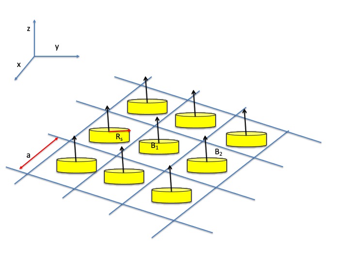
Our chosen two dimensional periodic magnetic field modulation is given by

$$\boldsymbol{B}=\Big[B_{2}+(B_{1}-B_{2})\sum_{m,n}\Theta(R_{s}-r_{mn})\Big]\boldsymbol{\hat{z}}$$

(5)

Here $R^{s}$ is radius of the circular region within each unit cell and $\boldsymbol{r}_{mn}=\boldsymbol{r}-\boldsymbol{R}_{mn}$ where $\boldsymbol{r}=x\boldsymbol{\hat{x}}+y\boldsymbol{\hat{y}}$. Apart from this, the lattice vector $\boldsymbol{R}_{mn}=ma\boldsymbol{\hat{x}}+na\boldsymbol{\hat{y}}$ and

$\displaystyle\Theta(R_{s}-r_{mn})$

$\displaystyle=$

$\displaystyle\begin{cases}1,~~\text{if}~\ r_{mn}\leq R_{s},\\ 0,~~\text{if}~\ r_{mn}>R_{s}\end{cases}$

(6)

where $m,n\in I(-N_{max},+N_{max})$ and $a$ denotes the lattice constant. We assume that the lattice constant $a$ is much larger than the carbon-carbon (c-c) bond length in bilayer graphene which justifies the consideration of continuum model for bilayer graphene. A schematic presentation of the magnetic field profile is given in Fig. 1. In general for any periodic magnetic field profile, because of the decomposition given in Eq. (4), the vector potential can be decomposed as

$$\boldsymbol{A}=\boldsymbol{A}_{u}+\boldsymbol{A}_{p}$$

with $A_{x}=A_{ux}+A_{px},~~A_{y}=A_{uy}+A_{py}$, where in a suitable gauge $\boldsymbol{A}_{p}$ can be written as a periodic function. Accordingly, for the current magnetic field profile given in Eq. (5) we have chosen a vector potential that has two parts, namely

	$\displaystyle\boldsymbol{A}_{u}(\boldsymbol{r})$	$\displaystyle=$	$\displaystyle\frac{1}{2}\boldsymbol{B}_{u}\times\boldsymbol{r},~\text{Symmetric Gauge}$
	$\displaystyle\boldsymbol{A}_{p}(\boldsymbol{r})$	$\displaystyle=$	$\displaystyle\frac{1}{2}\sum_{m,n}\Big[(B_{p}^{mn}\boldsymbol{\hat{z}})\times(r_{mn}\boldsymbol{\hat{r}}_{mn})\Big]$		(7)

where

$$B_{p}^{mn}=\begin{cases}\Big[(B_{1}-B_{2})-\frac{(B_{1}-B_{2})\pi(R_{s})^{2}}{a^{2}}\Big]\Theta(R_{s}-r_{mn}),\\ \text{if}\ r_{mn}\leq R_{s}\\ \\ (B_{2}-B_{1})\frac{\pi(R_{s})^{2}}{Na^{2}}\Theta(r_{mn}-R_{s}),~\text{otherwise}\end{cases}$$

(8)

Because of the periodic structure of the magnetic modulation given in Eq.(5), the resulting quasiparticle spectrum of Bernal stacked BLG subjected to such periodic magnetic modulation will be fundamentally different from the corresponding four band dispersion of the BLG without such magnetic modulation McCann. The uniform field $\boldsymbol{B}_{u}$ in the expression (4) will lead to Landau levels for such BLG Zarenia1, whereas the additional $\boldsymbol{B}_{p}$ field which forms a lattice of the magnetic modulation will convert these Landau levels into Hofstadter bands Hofstadter. It may be recalled that unlike in Moiré pattern in TBLG where a Hofstadter pattern arises MoireA; MoireB due to the presence of the Moiré periodicity that results from the relative twist between the two layers each of which is individually treated in continuum, in the present problem the periodic structure is provided by the periodic modulation of the magnetic field itself given in Eq. (5).

The eigenvalue equation for the hamiltonian given in (1) leads to the following set of coupled equations

	$\displaystyle v_{F}\Pi\psi_{b}$	$\displaystyle=$	$\displaystyle E\psi_{a}-v_{F}t\psi_{c}$		(9)
	$\displaystyle v_{F}\Pi^{\dagger}\psi_{a}$	$\displaystyle=$	$\displaystyle E\psi_{b}$		(10)
	$\displaystyle v_{F}\Pi^{\dagger}\psi_{d}$	$\displaystyle=$	$\displaystyle E\psi_{c}-v_{F}t\psi_{a}$		(11)
	$\displaystyle v_{F}\Pi\psi_{c}$	$\displaystyle=$	$\displaystyle E\psi_{d}$		(12)

We define $H_{G}=v_{F}^{2}\Pi\Pi^{\dagger}$. Since $H_{G}^{\dagger}=H_{G}$ coupling Eqs. (9) - (10), and Eqs. (11)-(12) we get

	$\displaystyle(H_{G}-E^{2})\psi_{a}$	$\displaystyle=$	$\displaystyle-v_{F}t\psi_{c}$		(13)
	$\displaystyle(H_{G}-E^{2})\psi_{c}$	$\displaystyle=$	$\displaystyle-v_{F}tE\psi_{a}$		(14)

The operator $H_{G}$ determines the energy spectrum for the monolayer graphene in the same periodic magnetic modulation. This tells us that $\psi_{a,c}$ will be obtained by solving the same eigenvalue equation upto an arbitrary phase factor like the MLG in a periodic magnetic modulation and $\psi_{b,d}$ can be obtained from Eqs. (10) and (12) subsequently for a given eigenvalue $E$. This is one of the major findings of this work, and has consequences like the topological quantisation of the Hall conductivity in magnetically modulated BLG which is studied in details in subsequent sections.

To get $\psi_{a,c}$ we combine Eqs. (13) and (14), giving

$$(H_{G}-E^{2})^{2}\psi_{a,c}=v_{F}^{2}t^{2}E^{2}\psi_{a,c}$$

(15)

Square-rooting of the above equation directly gives us the the eigenvalue spectrum $E$ of the BLG in the magnetic modulation defined in (5) as

$$\epsilon=\frac{1}{2}\bigg[\pm\frac{at}{\hbar}\pm\sqrt{(}\frac{a^{2}t^{2}}{\hbar^{2}}+4\epsilon_{M})\bigg]$$

(16)

where $\epsilon=\frac{aE}{\hbar v_{F}}$ and $\epsilon_{M}=\frac{a^{2}E_{M}^{2}}{\hbar^{2}v_{F}^{2}}$ are dimensionless energies in BLG and MLG respectively with $E_{M}$ representing the energy of the MLG modulated by the same magnetic modulation.It can be readily checked that for $t=0$, the expression (16) reduces to the corresponding spectrum of MLG in a way similar to the corresponding problem in uniform magnetic field case Zarenia1. The plots for the spectrum obtained using the above set of equations is shown in Fig. (2)- Fig. (6). In these plots the $x$-axis corresponds to $\alpha=\frac{p}{q}$ which is the total number of flux quanta through a unit cell and is given in terms of the co-prime $(p,q)$. $B_{1,2}$ defined in Eq. (5) is related to $\alpha$ through

$$\alpha\phi_{0}=B_{1}\pi R_{s}^{2}+B_{2}(a^{2}-\pi R_{s}^{2}).$$

(17)

And the $y$-axis corresponds to the dimensionless energy eigenvalue.

For a detailed analysis of the plots, we rewrite the LHS of Eq. (16) as $\epsilon_{+-,+-}$ where the first and second sign show the respective signs in the RHS of the spectrum. This implies that, $\epsilon_{+,+}$ and $\epsilon_{-,-}$ correspond to the two outer butterflies (blue and yellow in Fig 2) and $\epsilon_{+,-}$ and $\epsilon_{-,+}$ correspond to the two inner butterflies (green and red in Fig. 2)). For the case, when $\epsilon_{M}=0$, implying $\epsilon_{+,-}=\epsilon_{-,+}=0$, the two inner butterflies touch each other. This is the result obtained by setting interlayer coupling strength $t=400$ meV in Eq. (16).

As the value of $B_{1}$ is increased, the energy eigenvalue $\epsilon_{M}$ of the MLG in a similar magnetic modulation increases (see Fig. (4)). This causes increase in the the gap between the outermost butterflies $\epsilon_{+,+}$ and $\epsilon_{-,-}$. Similarly the gap between the inner butterflies $\epsilon_{+,-}$ and $\epsilon_{-,+}$ also increases with increase in $B_{1}$. This can be seen in the plots as we move from Fig (2) $(B_{1}=0)$ as well as in the leftmost figure of Fig. (4) $(B_{1}=1)$.

We now study the effect of fixing the value of magnetic field strength $B_{1}$ and varying the interlayer coupling strength $t$. The effect is demonstrated in Fig. (4). As $B_{1}$ is fixed, $\epsilon_{M}$ attains a fixed set of values. Going from left to right in Fig. (4), we can clearly observe that as t increases, the gap between the outer butterflies increases whereas the gap between the two inner butterflies decreases. This can be understood from Eq. (16), where as we increase t, the separation between $\epsilon_{+,+}$ and $\epsilon_{-,-}$ increases whereas that between $\epsilon_{+,-}$ and $\epsilon_{-,+}$ decreases. The spectrum is also plotted as a function of fixed value of $B_{2}$, but varying values of $B_{1}$ in Fig. (5) and Fig. (6).

Written in a slightly modified form, the eigenvalue equation for the BLG in a periodic magnetic modulation can be written in terms of the corresponding hamiltonian operator for the MLG as

$$H_{G}\psi_{a,c}=\big[(E^{\pm})^{2}-\frac{1}{4}v_{f}^{2}t^{2}\big]\psi_{a,c}$$

(18)

where $E^{\pm}=E\pm\frac{1}{2}v_{f}t$. It is known that $H_{G}$ commutes with the magnetic translation operator Zak corresponding to the uniform field part of the magnetic modulation, namely $B_{u}$. Hence the eigenfunctions of the $H_{G}$, which are also the magnetic Bloch functions, can be expanded in terms of localised Wannier functions in the presence of uniform transverse magnetic field $\boldsymbol{B}_{u}$Luttinger; Wannier.

$$\psi_{\boldsymbol{k}}^{a,c}=\sum_{i}g(\boldsymbol{R}_{i})\exp\big(-i\frac{e\boldsymbol{A}_{u}\cdot\boldsymbol{R}_{i}}{\hbar c}\big)w_{0}(\boldsymbol{r}-\boldsymbol{R}_{i})$$

(19)

To simplify further calculation here we set the condition $|\frac{ea^{2}}{\hbar c}(B_{u}+B_{p})|<<1$. For $B_{p}=0$, this implies $|\frac{ea^{2}}{\hbar c}(B_{u})|\ll 1$ which leads to $a\ll l_{B_{u}}$. Here $l_{B_{u}}$ is the magnetic length which is defined in terms of the uniform part of the magnetic modulation. Thus this condition corresponds to a weak and slowly varying magnetic field Luttinger; exact. This is a reasonable approximation as long as the modulation part $B_{p}$ ( represented by either the r.m.s value, or the peak value) is smaller than $B_{u}$, and hence, can be treated as a perturbative effect. This type of condition is generally used in lattice gauge theory Governale. Under these approximations we can write the eigenvalue equation ($\ref{MLGBLG})$ as a discrete Schrödinger equation which takes the form of Hofstadter-Harper equation

	$\displaystyle\epsilon g(m,n)$	$\displaystyle=$	$\displaystyle e^{\frac{iea}{\hbar c}(A_{ux}+A_{px})}g(m+1,n)+e^{-\frac{iea}{\hbar c}(A_{ux}+A_{px})}g(m-1,n)+e^{\frac{iea}{\hbar c}(A_{uy}+A_{py})}g(m,n+1)$		(20)
		$\displaystyle+$	$\displaystyle e^{-\frac{iea}{\hbar c}(A_{uy}+A_{py})}g(m,n-1)-[\frac{ea^{2}}{\hbar c}(B_{u}+B_{p})+4]g(m,n)$

with

$$\epsilon=-\frac{[(E^{\pm})^{2}-\frac{1}{4}v_{f}^{2}t^{2}]a^{2}}{v_{F}^{2}\hbar^{2}}$$

(21)

and $g(m,n)=g(\boldsymbol{R_{mn}})$.

Once $\psi_{a,c}$ is calculated from Eqs. (19) and (20), using Eq. (10) we can calculate ( again under the weak magnetic field limit)

	$\displaystyle\psi_{\boldsymbol{k}}^{b}$	$\displaystyle=$	$\displaystyle\frac{v_{F}}{E}\bigg[-i\hbar(\frac{\psi_{\boldsymbol{k}}^{a}(\boldsymbol{r}+a\boldsymbol{\hat{x}})-\psi_{\boldsymbol{k}}^{a}(\boldsymbol{r}-a\boldsymbol{\hat{x}})}{2a})$		(22)
		$\displaystyle-$	$\displaystyle i\hbar(\frac{\psi_{\boldsymbol{k}}^{a}(\boldsymbol{r}+a\boldsymbol{\hat{y}})-\psi_{\boldsymbol{k}}^{a}(\boldsymbol{r}-a\boldsymbol{\hat{y}})}{2a})$
		$\displaystyle+$	$\displaystyle\frac{e}{c}(A_{u}^{x}+iA_{u}^{y}+A_{p}^{x}+iA_{p}^{y})\psi_{k}^{a}(\boldsymbol{r})\bigg]$

In a similar manner $\psi_{\boldsymbol{k}}^{d}$ also can be determined from $\psi_{\boldsymbol{k}}^{c}$. Thus all the eigenfunctions can be determined.

In the previous section we studied the BLG spectrum in a periodic magnetic modulation using the four-band model. In several BLG problems, an effective two-band model is used Geimbilayer; Falkobilayer to analyse the behaviour of the charge carriers in BLG in an external field. In such two-band model, the low energy hamiltonian in effective-mass approximation is further projected on the lowest two energy bands McCann. In this section we shall study the magnetically modulated BLG spectrum using this effective two-band model within the framework of our algebraic approach.

Using the form of the effective $2\times 2$ hamiltonian at low energies for BLG charge carriers in the presence of 2d periodic magnetic modulation, we can write the eigenvalue equation as

$$\displaystyle\frac{1}{2m}\left[{\begin{array}[]{cc}0&(\Pi^{\dagger})^{2}\\ (\Pi)^{2}&0\\ \end{array}}\right]\begin{bmatrix}\psi_{1}\\ \psi_{2}\end{bmatrix}=E\begin{bmatrix}\psi_{1}\\ \psi_{2}\end{bmatrix}$$

Using the commutator

$$[\Pi^{\dagger},\Pi]=\frac{2\hbar e}{c}(B_{u}+B_{p})$$

(25)

a straightforward decoupling yields (we retain the same notation for the hamiltonian and the energy eigenvalues)

$$H\psi_{1}=E^{2}\psi_{1}$$

(26)

with

	$\displaystyle H$	$\displaystyle=$	$\displaystyle\frac{1}{4m^{2}}(\Pi^{\dagger})^{2}(\Pi)^{2}=\frac{1}{4m^{2}}(\Pi^{\dagger})\Big([\Pi^{\dagger},\Pi]+\Pi\Pi^{\dagger}\Big)(\Pi)$		(27)
		$\displaystyle=$	$\displaystyle\frac{1}{4m^{2}}\Big[\frac{H_{G}^{2}}{v_{F}^{4}}+\Big(\frac{2\hbar e}{c}(B_{u}+B_{p})\Big)\frac{H_{G}}{v_{F}^{2}}+\frac{2\hbar e}{c}\Big(\Pi^{\dagger}(B_{u}+B_{p})\Big)\Pi\Big]$

Under the approximation that the magnetic field is weak and slowly varying, we can ignore the last term appearing in the above hamiltonian which invokes the following argument. In the current problem $B_{u}+B_{p}=B(\vec{r})$ is spatially constant both inside and outside circular regions, whereas at the boundary of the two regions it is a step function and hence strictly speaking it’s derivative will give discontinuity in the form of a delta function. But in reality there will be an intermediate region where the magnetic field will smoothly go from $B_{1}$ to $B_{2}$ over a finite region that is sufficiently large as compared to the bond-length of graphene, but sufficiently small compared to the relevant length scales that appear in the current problem. Therefore we can set

$$\Big(p_{x}-ip_{y}\Big)\Big(B_{u}+B_{p}\Big)\approx 0$$

(28)

throughout the considered region. Moreover, we also impose the condition $|\frac{ea^{2}}{\hbar c}B(\vec{r})|\ll 1$ and $|\frac{eaA_{x,y}}{\hbar c}|\ll 1$. Given this

$$\frac{2a^{4}e}{\hbar^{3}c}\Big(\Pi^{\dagger}(B_{u}+B_{p})\Big)\Pi\\ =\frac{2a^{4}e}{\hbar^{3}c}\Big[\Big(p_{x}-ip_{y}\Big)\Big(B_{u}+B_{p}\Big)+\Big(\frac{e}{c}(A_{x}-iA_{y})\Big)\Big(B_{u}+B_{p}\Big)\Big]\Pi\approx=0$$

(29)

The hamiltonian $H$ can therefore be approximated as

$$H\approx\Big[\frac{H_{G}^{2}}{v_{F}^{4}}+\Big(\frac{2\hbar e}{c}(B_{u}+B_{p})\Big)\frac{H_{G}}{v_{F}^{2}}\Big]=H^{\prime}$$

(30)

and the eigenvalue equation to be solved is

$$H^{\prime}\psi_{1}=4m^{2}E^{2}\psi_{1}$$

Since $[H^{\prime},H_{G}]=0$, $\psi_{1}$ can be taken same as the eigenfunction of $H_{G}$. The other component of the spinorial wavefunction $\psi_{2}$ can be written as

$$\psi_{2}=\frac{1}{2mE}\hat{\Pi}^{2}\psi_{1}$$

(31)

$E$ can now be determined as

$$E=\pm\frac{\hbar^{2}}{2ma^{2}}\sqrt{\epsilon_{M}^{2}+4\pi\frac{(B_{u}+B_{p})a^{2}}{\phi_{0}}\epsilon_{M}}$$

(32)

$\epsilon_{M}$ is the dimensionless energy of the MLG in the same magnetic modulation. It is interesting to note that similar to the case of dispersion obtained from the effective two-band low energy description of BLG, here also the energy scales in the unit of $\frac{\hbar^{2}}{2ma^{2}}$. We can therefore set the dimensionless energy here as $\epsilon=\frac{E}{\frac{\hbar^{2}}{2ma^{2}}}$. This points out to the fact that the quasiparticles are massive, unlike the case of magnetically modulated MLG where the quasiparticles are massless. The energy spectrum is also plotted in the same unit in Fig. 7. In this case we get two copies of the Hofstadter butterfly spectrum which is consistent with the two-band approximation. The analytical form of the energy spectrum in a magnetically modulated Bernal stacked BLG, derived respectively under four band and the two band approximation and given in Eq. (16) and Eq. (32), forms one of the major result in this work.

The spectrum presented in Figs. 2, 4, 4, 5, 6, 7 are all enumerated with the help of Eq. (20) which is a discrete eigenvalue equation. This is derived from the eigenvalue Eq. 18 by first expanding the solutions in terms of gauged Wannier functions defined in Eq. (19) and then using the nearest neighbour tight-binding approximation. As a result, for the MLG spectrum we obtained only two copies of the Hofstatdter butterflies both of which are bounded, and the BLG spectrum was obtained using the expression from the MLG spectrum by use of relation (16) and Eq. (32). It may be recalled BookChap that the eigenvalue equation (20) is similar in form to the celebrated Harper equation Harper that was obtained in the original work of Hofstadter Hofstadter, by considering the single lowest band of Bloch equation in the presence of a uniform magnetic field. In absence of the magnetic field, the band dispersion for such a single band in a square lattice periodic potential in the tight binding approximation is given by

$$E(k_{x},k_{y})=2t(\cos k_{x}a_{sl}+\cos k_{y}a_{sl})$$

(33)

where $k_{x},k_{y}$ are Bloch momentums along $x,y$ directions respectively, $t$ is the energy scale set by hopping and $a_{sl}$ is the lattice constant of the square lattice. As can be seen from this expression, the width of such single band is finite, resulting in the finiteness of the energy spectrum given by the Hofstadter butterfly when the effect of a uniform magnetic field is added through Peierls’ substitution. This situation may be contrasted carefully with the approach in the current problem where we start from the low-energy dispersion of Bernal-stacked bi-layer graphene or monolayer graphene in the $\boldsymbol{k}\cdot\boldsymbol{p}$ approximation that are respectively quadratic McCann and linear Novoselov1 in quasi (Bloch)-momentum and hence unbounded. When a periodic magnetic modulation given by Eq. 4 is added to such problem, it is expected that the resulting spectrum should show higher energy copies of the Hofstadter butterflies corresponding to the higher-energy part of the spectrum of the unperturbed problem. However, as can be seen, the spectrum presented in Figs. 2, 4, 4, 5, 6, 7 are all bounded.

The absence of these higher energy copies in our calculation can be explained by noting our restriction to the nearest neighbour tight-binding which is clearly visible in the form of Eq. (20). Here we first provide a brief justification for ignoring the higher order terms in the tight-binding approximation. Then we shall write some comments about how such restrictions can be relaxed and more accurate spectrum can be obtained. As already mentioned that in the current problem we use the weak field limit $a\ll\ell_{B_{u}}$, where $a$ accounts for the periodicity of the periodic magnetic modulation studied here. Even though the effective bilayer graphene hamiltonian is continuous and hence unbounded, the lattice present due to the periodic modulation justifies the discretisation and the nearest neighbour truncation of the resultant equation under this weak field limit. A single dispersion like Eq. (33) for the current problem by considering only the $\boldsymbol{B}_{p}$ in Eq. 4 is also a non-trivial problem, because the lattice parameter $a$ here is not the carbon-carbon bond length, and is purely due to the magnetic modulation. To extend the current calculation in the strong field limit (where the magnetic length is comparable or may be even lower than the lattice-spacing) one can follow the methods described in ref. Janecek where the Scrhödinger equation in a periodic potential and magnetic field is numerically diagonalised exploiting the magnetic translational symmetry of the problem. Alternatively one can use the method adopted in ref. Gumbs by first solving the corresponding problem in an uniform magnetic field Zarenia1 and then applying the zero-flux periodic magnetic modulation represented by the fiield $B_{p}\hat{z}$ as a perturbation. Direct relaxation of our scheme can also be used, however a comparison between these various schemes is not clear at this stage. All these methods are numerically demanding and we hope to address some of them in future work.

References

- (1) K. S. Novoselov et al. Nat. Phys. 2, 177 (2006);
- (2) R. D. Hofstadter, Phys. Rev. B 14, 2239 (1976).
- (3) D. J. Thouless, M. Kohmoto, M. P. Nightingale, and M. den Nijs, Phys. Rev. Lett. 49, 405 (1982).
- (4) Mahito Kohmoto, Annals of Physics 160, 343-354 (1984).
- (5) K. v. Klitzing, G. Dorda, and M. Pepper, Phys. Rev. Lett. 45, 494 (1980).
- (6) J. Zak, Phys. Rev. A: Gen. Phys. 134, 1607 (1964).
- (7) H. J. Fischbeck, Phys. Status Solidi 38, 11 (1970).
- (8) W. Florek, Act. Phys. Pol. A 92, 399-402 (1997).
- (9) A. Ghazarayan and T. Chakraborty, Phys. Rev. B 91, 125131 (2015).
- (10) M. Arora and S. Ghosh, Phys. Rev. B 98, 155425 (2018).
- (11) K. S. Novoselov, A. K. Geim, S. V. Morozov, D. Jiang, M. I. Katnelson, I. V. Grigorieva, S. V. Dubonos, and A. A. Firsov, Nature(London) 438, 197 (2005).
- (12) V. P. Gusynin and S. G. Sharapov, Phys. Rev. Lett. 95, 146801 (2005)
- (13) S. B. Trickey, F. Müller-Plathe, G. H. F. Diercksen and J. C. Boettger, Phys. Rev. B 45, 4460 (1992).
- (14) J. R. Wallbank, M. M-Kruczyński, X. Chen and V. I. Fal’ko, Annalen der Physik, 527, 359 (2015).
- (15) C. R. Dean et al., Nature, 497, 598 (2013).
- (16) G. L. Yu et al., Nature Physics, 10, 525 (2014).
- (17) A. Ghazarayan and T. Chakraborty, Phys. Rev. B 92, 235404 (2015).
- (18) Z.. F. Wang, F. Liu and M. Y. Chou, Phys. Rev. B, 12, 3833 (2012)
- (19) E. McCann and M. Koshino, Rep. Prog. Phys, 76, 056503 (2013).
- (20) E. McCann and V.I. Fal’ko, Phys. Rev. Lett. 96, 086805 2006.
- (21) K.S. Novoselov et al. Nat. Phys. 2, 620 (2006).
- (22) A.F. Young and P. Kim, Nat. Phys. 5, 222, (2009); N. Stander, B. Huard, and D. Goldhaber-Gordon, Phys. Rev. Lett. 102, 026807 (2009); A.F. Young and P. Kim, Ann. Rev. Cond. Matt. Phys. 2 1-20 (2010).
- (23) L. Z. Tan, C-H Park and S. G. Louie, Nano Lett. 2011, 11, 2596 (2011).
- (24) M.I. Katsnelson and K.S. Novoselov, Sol. St. Comm. 143, 3 (2007).
- (25) M. R. Masir, P. Vasilopoulos and F. M. Peeters, Phys. Rev. B, 79, 035409 (2009).
- (26) N. Gu, M. Rudner and L. Levitov, Phys. Rev. Lett., 107, 156603 (2011).
- (27) N. Agrawal(Garg), S. Grover, S. Ghosh and M. Sharma, J. Phys.: Condens. Matter, 24, 175003 (2012).
- (28) M. Zarenia, P. Vasilopoulos and F. M. Peeters, Phys. Rev. B 85, 245426 (2012).
- (29) R. Bistritzer and A. H. MacDonald, Phys. Rev. B, 84, 035440 (2011).
- (30) B. Lian, F. Xie and B. Andrei Bernevig, Phys. Rev. B 103, L161405 (2021).
- (31) U. Rössler and M. Suhrke, Bloch Electrons in a Magnetic Field: Hofstatder’s Butterfly, Book Chapter in Advances in Solid State Physics, 40, 35 (2000).
- (32) P. G. Harper, Proc. Phys. Soc. (London), A270, 1 (1962).
- (33) S. Janecek, M. Aichinger and E. R. Hernández, Phys. Rev. B 87, 235429 (2013).
- (34) G. Gumbs, A Iurov, D. Huang and L. Zhemchuzna, Phys. Rev. 89, 241407 (2014).
- (35) M. Zarenia, J. M. Pereira Jr., G. A. Farias and F. M. Peeters, Physical Review B, 84, 125451 (2011).
- (36) J. M. Luttinger, Phys. Rev. 84, 814 (1951).
- (37) G. H. Wannier and D. R. Fredkin, Phys. Rev. 125, 1910 (1962).
- (38) S. Janecek, M. Aichinger and E. R. Hernandez, Phys. Rev. B 87, 235429 (2013).
- (39) M. Governale and C. Ungarelli, Phys. Rev. B 58, 7816 (1998).
- (40) E. McCann, Phys. Rev. B, 74 161403 (2006)
- (41) E. V. Castro et al. Phys. Rev. Lett., 99 216802 (2007)
- (42) S. D. Bader, Rev. Mod. Phys. 78, 1 (2006)
- (43) J. G. Park, Jour Phys. Cond. Matt. 28, 301001 (2016).
- (44) B. N. Soskic, S. Stavric and Z. Sljivancanin, Phys. Rev. Materials, 5, 074001 (2001).
- (45) J. Mao et al., Nature 584, 215 (2020).
- (46) R. Banerjee et al., Nano Lett. 20, 3113 (2020).
- (47) L. R. S. Marie et al. Phys. Rev. B 104, 085435(2021)