Determining the bubble nucleation efficiency of low-energy nuclear recoils in superheated C3F8 dark matter detectors
Abstract
The bubble nucleation efficiency of low-energy nuclear recoils in superheated liquids plays a crucial role in interpreting results from direct searches for weakly interacting massive particle (WIMP) dark matter. The PICO collaboration presents the results of the efficiencies for bubble nucleation from carbon and fluorine recoils in superheated C3F8 from calibration data taken with five distinct neutron spectra at various thermodynamic thresholds ranging from 2.1 to 3.9 keV. Instead of assuming any particular functional forms for the nuclear recoil efficiency, a generalized piecewise linear model is proposed with systematic errors included as nuisance parameters to minimize model-introduced uncertainties. A Markov chain Monte Carlo (MCMC) routine is applied to sample the nuclear recoil efficiency for fluorine and carbon at 2.45 and 3.29 keV thermodynamic thresholds simultaneously. The nucleation efficiency for fluorine was found to be for nuclear recoils of 3.3 keV (3.7 keV) at a thermodynamic Seitz threshold of 2.45 keV (3.29 keV), and for carbon the efficiency was found to be for recoils of 10.6 keV (11.1 keV) at a threshold of 2.45 keV (3.29 keV). Simulated datasets are used to calculate a p value for the fit, confirming that the model used is compatible with the data. The fit paradigm is also assessed for potential systematic biases, which although small, are corrected for. Additional steps are performed to calculate the expected interaction rates of WIMPs in the PICO-60 detector, a requirement for calculating WIMP exclusion limits.
I Introduction
Superheated liquids are excellent targets for direct dark matter detection experiments searching for heavy dark matter particles such as weakly interacting massive particles (WIMPs) scattering off atomic nuclei. The nuclear recoil (NR) that is predicted to result from such a scatter creates a single bubble at the interaction site in the superheated target. World-leading limits have been set on dark matter-nucleus scattering rates based on the observed absence of such bubble nucleation Behnke et al. 2012; Amole et al. 2015; Amole et al. 2016; Amole et al. 2017; Amole et al. 2019a; Behnke et al. 2017. In the interpretation of these (and future) experimental results, the bubble nucleation efficiency for NRs as a function of both the thermodynamic state of the chamber and the nuclear recoil energy, is crucial to determining dark matter sensitivity. To characterize this detector response, neutrons are used as proxies for dark matter particles, generating the same NR-induced bubbles as expected from dark matter, but with few-cm mean-free paths and recoil energy spectra that depend on the incident neutron energy. This paper presents results from the PICO collaboration’s campaign over nearly a decade using a variety of neutron sources to calibrate the low-energy (keV-scale) nuclear recoil sensitivity of superheated C3F8.
I.1 Bubble nucleation by nuclear recoils
The thermodynamic basis for bubble nucleation by nuclear recoils is described by Seitz’s “hot-spike” model Seitz 1958, a detailed modern treatment of which is given in Amole et al. 2019b, summarized here. This model is based on two well-defined thermodynamic quantities, the critical radius and the energy threshold . is the radius above which vapor bubbles in the superheated fluid will spontaneously grow, eventually becoming the macroscopic bubbles observed by experiments such as PICO. The critical radius is given by
| (1) |
where is the surface tension of the fluid, is the pressure of the vapor filling the bubble, which is approximately equal to the saturation pressure of the fluid at the operating temperature (controlled experimentally), and is the pressure of the superheated liquid in the bubble chamber (also controlled experimentally). In Seitz’s model, nuclear recoils create this critical proto-bubble by locally heating the fluid, and the amount of heat required to create a critically sized proto-bubble is referred to as the Seitz threshold, given by
| (2) |
Here, is the density of the vapor filling the bubble, and and are the specific enthalpies of the gaseous and liquid states. The three terms in represent the energy needed to create the bubble surface, the energy required to vaporize fluid to fill the bubble interior, and the recapture of reversible work present in both of the first two terms. Any particle interaction injecting heat greater than (3 keV in the experiments considered here) into a volume small compared to (25 nm) will create a critically sized proto-bubble, which will then grow to the macroscopic bubble detected in these experiments.
As a consequence of this idealized model, the efficiency for bubble nucleation would be a step function from 0% to 100% when the energy deposited within a critical length scale exceeds the Seitz threshold:
| (3) |
where is a unitless scale factor of , often referred to as the “Harper” parameter Harper 1993. For low-energy nuclear recoils, this would simplify further to (all recoil energy deposited within the critical scale), and a calculation of from the temperature and pressure of the superheated target would be sufficient to determine the nuclear recoil detection threshold. Unfortunately, this is not true for at least three reasons. First, Eq. (2) does not include corrections to surface tension at a small radius of curvature, an effect described by the Tolman length Tolman 1949 and covered in detail in Amole et al. 2019b. The Tolman length itself is unknown and leads to -keV uncertainties in . Second, does not account for energy losses that do not contribute to local heating, such as radiative losses (e.g. fluorescence), and irreversible work (e.g. acoustic radiation), or thermal diffusion transporting heat outside critical radius. Finally, and most importantly, Eq. (3) does not reflect event-to-event variation in track structure (i.e. straggling in ) which simulations using SRIM Ziegler et al. 2010 show to be significant in nuclear recoils at the energies and length scales considered here.
The effects above can both shift the nuclear recoil detection threshold and, in the case of straggling, broaden it, leading to detection efficiencies below 100% near the threshold. Indeed, past data with measured monoenergetic recoils d’Errico 1999; d’Errico 2001; Tardif 2018 demonstrate that the nucleation threshold is not an ideal step function. Since there is no quantitative theory to describe these effects, past efforts have invoked ad hoc parametrizations for the threshold function, such as an exponential Archambault et al. 2011; Behnke et al. 2012; Behnke et al. 2013, a sigmoid function Tardif 2018 and a “superheated factor” Lo and Apfel 1988; Felizardo et al. 2010. Efforts remain to understand and explain the processes that contribute to the resolution function that shifts and convolutes the Seitz step threshold Tardif 2018. Until these effects are fully understood, nucleation efficiencies must be determined by performing dedicated neutron calibrations, as described in this work.
The following sections comprise a global analysis of the PICO collaboration’s neutron calibrations to date in superheated C3F8, the target fluid for the PICO-2L, PICO-60, PICO-40L, and PICO-500 dark matter searches. The general calibration scheme, the specific experimental setups used, and the resulting data and corresponding simulations are described in Sec. II. Section III describes the methods used to extract bubble nucleation efficiencies from this data, including the parametrization of the efficiency function, treatment of systematic uncertainties as nuisance parameters, and the specific Markov chain Monte Carlo (MCMC) technique used to explore the resulting high-dimensional parameter space. Section IV describes a parametric Monte Carlo study validating the methodology created for this analysis. Appendices describe the application of this technique to directly constrain WIMP sensitivity in the PICO experiments and present an evaluation of and correction for any bias introduced in this analysis.
II Calibration Program – Data and Simulations
The objective of the PICO C3F8 nuclear recoil calibration program is to constrain the bubble nucleation efficiency functions , where is the probability of bubble nucleation, indicates the recoil species (carbon or fluorine), is the thermodynamic threshold set by the pressure and temperature of the chamber (equal to as calculated in Amole et al. 2019b), and is the nuclear recoil energy. Specifically, we aim to constrain the dependence of these functions at the fixed various employed in the PICO dark matter searches. Constraints on come from rate measurements in bubble chambers exposed to known neutron sources. In general, these constraints take the form of a convolution of the underlying recoil spectrum with the efficiency curve:
| (4) |
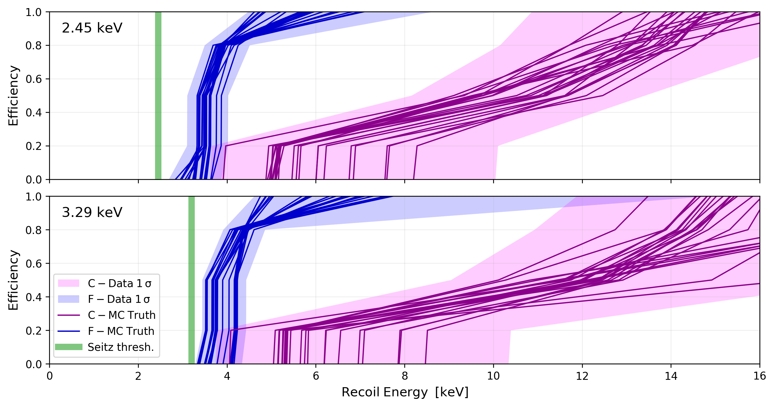
where is the experimentally observed rate and the are the nuclear recoil spectra (by species) due to the neutron source, determined from simulation.
A single constraint in Eq. (4) is insufficient to deduce the underlying and , as the convolution cannot indicate which recoils are nucleating bubbles – i.e. threshold shift is indistinguishable from a soft threshold. A suite of measurements with sources producing different recoil spectra, however, is capable of making this distinction. The ability to reconstruct multiple-scattering events in calibration experiments is also key. Each experiment produces not a single rate measurement but a set of measurements giving the one-bubble event rate, two-bubble event rate, etc., with each multiplicity effectively probing a different underlying recoil spectrum. In this sense, Eq. (4) is a simplification applying only to the single-bubble rate in a chamber much smaller than the neutron mean-free path, which is not the case in the measurements presented here. Finally, the dependence of the efficiency curves can be explored by varying the thermodynamic state of a calibration chamber. However, unless assumptions are made relating to the and dependence of the efficiency function, this does little to constrain dependence at the of interest.
II.1 Neutron interactions in C3F8
Neutrons interact predominantly by elastic scattering off of 12C and 19F nuclei (with % 13C) in the C3F8 target. The energy spectrum of the recoiling nuclei is described by
| (5) |
where is the atomic mass of the recoiling nucleus, is the neutron scattering angle in the center of mass frame, and En is the incident neutron energy. By fixing = , the maximum recoil energies are = 0.28 and = 0.19 for carbon and fluorine respectively. When the incoming neutrons are monoenergetic and the scattering is isotropic, this produces the recoil spectra and rate over threshold shown in Fig. 1.

Actual neutron-carbon and neutron-fluorine cross sections are shown in Fig. 2, illustrating three resonances in the neutron-fluorine scattering cross section in the energy scale of interest. By calibrating with monoenergetic neutrons at energies on and off these resonances, it is possible to vary the relative rates of carbon and fluorine scattering, allowing separate calibration of and . It should be noted that on-resonance scattering is not isotropic, so at these energies, the fluorine recoil spectra deviate from the idealized box-shaped spectrum in Fig. 1 Robinson 2014.

II.2 Experimental setup
II.2.1 Detectors
Two detectors have been employed in the PICO C3F8 nuclear recoil calibration program: the PICO-2L detector at SNOLAB, described in Amole et al. 2015, and a portable version, the PICO-0.1L test bubble chamber, described in Amole et al. 2019b. Designed to accomplish calibrations that are difficult in larger chambers, PICO-0.1L consists of a 100-mL, centimeter-thick high-pressure-rated quartz jar attached to a hydraulically driven bellows and immersed in a chilled water bath. The quartz vessel is filled with 27 1 gram of C3F8 (19.4 mL of fluid at a density of 1.39 g/mL at 12∘C and 30 psia), as measured by a scale, where the uncertainty is due to losses in the fill lines and the resolution of the scale readout. The remaining space in the vessel is filled with a water buffer, both to create an incompressible volume for pressure control and to avoid any contact between the superheated C3F8 target and the stainless steel surfaces and seals in the bellows system. Bubble nucleation events are recorded by two piezoelectric acoustic sensors mounted on the jar and by two cameras (150 frames/s) located at 90 degrees from each other. Two LED panels alternate to illuminate the chamber, each in synchronization with one of the cameras. The PICO-0.1L vessel is shown in Fig. 3, both alone and with the attached imaging and pressure- and temperature-control systems.

II.2.2 Neutron sources and neutron monitor
PICO-0.1L was deployed from 2013 to 2019 at the Van de Graaff Tandem accelerator facility at Université de Montréal, where data were taken both with monoenergetic neutron beams produced by the accelerator and with a SbBe photoneutron source. PICO-2L operated at SNOLAB, with periodic neutron calibrations performed using an AmBe source during the dark matter search.
Monoenergetic neutron beam
Monoenergetic neutrons were produced with the Tandem Van de Graaff accelerator via the reaction 51V(p,n)51Cr Gibbons et al. 1955; Lafreniere 2018. The energies of the neutrons produced by this reaction are the proton energy minus 1564 keV, the Q value of the reaction so that a monoenergetic proton beam and thin target produce a monoenergetic neutron beam. The energy resolution of the neutron beam is significantly enhanced when the proton energy is at one of the many sharp resonances shown in Fig. 4. The data considered here were taken at resonances VII, VIII, and XI, corresponding to neutron energies of 50, 61, and 97 keV, respectively. These three 51V(p,n)51Cr resonances were chosen to align on and between the neutron scattering resonances shown in Fig. 2, with the 50- and 97-keV neutrons on resonance and the 61-keV neutrons off resonance for scattering on fluorine.

Figure 5 illustrates the experimental setup for neutron beam data. The PICO-0.1L test chamber sits directly downstream of the 51V target, with a penetration through the chilled water bath giving neutrons a direct path to the quartz vessel. The details of this penetration changed between the 2013 and 2014 datasets, as reflected in the analysis in Sec. III. Two 3He neutron counters monitor the beam flux, one immediately below the 51V target and one below the PICO-0.1L water bath. These counters provide the neutron flux normalization described in Sec. II.5 and provide live feedback to ensure that the proton beam stays at the peak of the selected 51V(p,n)51Cr resonance during data taking.

Monoenergetic SbBe photoneutrons
To study the detector response at lower recoil energies with the PICO-0.1L test chamber, additional calibration runs were performed using a SbBe photoneutron source, a two-component source that contains a 124Sb gamma source and a 9Be conversion target, producing neutrons via the 9Be(,n) reaction Collar 2013; Robinson 2016. There are two significant gamma rays emitted by 124Sb above the 1665-keV Q value of this reaction: 1691 and 2091 keV, with branching ratios of 48.4% and 5.7%, producing 24 and 378 keV neutrons, respectively. A challenge with this calibration is that the source emits (106) higher gamma flux than neutron flux. While PICO bubble chambers are in general gamma blind Amole et al. 2019b, the detector does start to become gamma sensitive at Seitz thresholds below 3 keV, increasing the single-bubble event rate. This gamma response is measured by removing the beryllium disk and is considered in the analysis as a background to the SbBe response of the detector. Throughout the measurements, two one-inch thick lead disks were inserted in front of the SbBe source to attenuate the gamma flux, but the gamma-induced single-bubble rate was still deemed too high for useful analysis, and therefore only multibubble events are considered from the SbBe exposure. The setup for the calibration with the SbBe source (without lead attenuators) is shown in Fig. 6.

AmBe neutrons
Neutron calibration with an AmBe source was carried out at SNOLAB with the PICO-2L detector filled with C3F8. In contrast to the monoenergetic neutron sources above, this broad-spectrum source of (1)-MeV neutrons generates nuclear recoils far above the detector threshold. The threshold-constraining power of this measurement comes from the high-statistics, low-background measurement of high-multiplicity events (up to six bubbles and beyond) captured in the two-liter target. Moreover, the different detector, source, and style of constraint provided by this dataset serve as an important check on the systematic uncertainties associated with each of the neutron calibrations performed.
II.3 Data quality and preparation
Each calibration dataset is reduced to a small set of parameters for subsequent analysis. These parameters include the thermodynamic threshold of the bubble chamber (), total live-time at that threshold, number of events observed (separated by bubble multiplicity), and background bubble rate (also separated by bubble multiplicity) measured without the source/beam in each setup. The background data (dominated by cosmogenic neutrons) was always taken close in time to the corresponding experiment. In the case of the beam experiments, the background rate was found to be consistent over time. For all experiments except for the SbBe data (see paragraph 2b in the previous subsection), it is assumed that gammas from the beam/source produce a negligible background, as the bubble chambers were operated in thermodynamic conditions well beyond the measured electron recoil threshold Amole et al. 2019b. The datasets are summarized in Table 1, and the measured background-subtracted event rates as a function of threshold are shown in Fig. 7.
The above data reduction is performed largely by hand; camera images are visually inspected (hand scanned) to verify bubble counts, a process that is taken to be 100% efficient. A series of quality cuts are also applied to eliminate regions in time and/or regions in the detector where chamber performance is compromised. These cuts include the removal of runs where pressure or temperature control was not functioning as intended; the removal of the first 10 (30) seconds in every PICO-0.1L (PICO-2L) expansion, to allow time for the chamber to reach equilibrium; a fiducial cut in PICO-2L as described in Amole et al. 2015, applied to single-bubble events only; and a fiducial cut in 2013 PICO-0.1L data, removing both single- and mutliple-bubble events where a bubble appears in the top cm of the target (which in that run became excessively foamy). The fiducial cuts in PICO-2L and PICO-0.1L are applied to simulated data as well as to real data.
| Dataset | Detector | Thresholds | Live-time | Multiplicity |
| (keV) | (minutes) | |||
| 97 keV beam | PICO-0.1-2013 | 3.2 | 9.9 | 1,2,3+ |
| 61 keV beam | PICO-0.1-2013 | 3.1 | 160 | 1,2,3+ |
| 97 keV beam | PICO-0.1-2014 | 3.0, 3.6 | 21, 20 | 1,2,3+ |
| 61 keV beam | PICO-0.1-2014 | 2.9, 3.6 | 16, 18 | 1,2,3+ |
| 50 keV beam | PICO-0.1-2014 | 2.5, 3.0, | 3.1, 7.7, | 1,2,3+ |
| 3.5 | 7.3 | |||
| SbBe | PICO-0.1 | 2.1, 2.6, | 320, 310, | 2,3+ |
| 3.2 | 300 | |||
| AmBe | PICO-2L | 3.2 | 2200 | 1,2,3,4, |
| 5,6,7+ |
II.4 Simulations of neutron scattering
For each neutron calibration dataset, a GEANT4 Agostinelli et al. 2003 (SbBe and AmBe data) and/or MCNP-POLIMI Pozzi et al. 2003 (beam and AmBe data) Monte Carlo simulation is performed to provide the recoil energy spectra for single- and multiple-scatter events within the detector. These are used, in conjunction with hypothesized bubble nucleation efficiency functions, to calculate the expected event rate by bubble multiplicity for each calibration experiment. Neutron scattering cross sections for both transport through the geometry and signal production in the detector are taken from Evaluated Neutron Data File ENDF/B-VII Brown et al. 2018 for both MCNP and GEANT4 Mendoza and Cano-Ott 2018, with corrections from Robinson 2014 for the differential scattering cross sections at the fluorine resonances, which ENDF incorrectly treats as s-wave (isotropic).
Each of the three neutron sources considered requires a slightly different treatment for particle generation. For the beam simulations, the energy-angle relation for neutrons coming from the 51V(p,n)51Cr reaction is included directly in the MCNP-POLIMI neutron source definition, based on data in Gibbons et al. 1955. A similar energy-angle relation exists for the SbBe photoneutron source, but because the Sb gammas are emitted isotropically into a large Be target, a simple neutron source definition capturing this relation is not possible. Furthermore, this relation cannot be simulated natively in MCNP-POLIMI – while MCNP-POLIMI does simulate the 9Be(,n) reaction, it does so by treating the incoming photon as a zero-momentum particle, and therefore misses the angular dependence of the resulting neutron energy. To address this shortcoming, a photon-only simulation of the Sb source and Be target was run and neutron production was inserted manually to generate a list of neutrons with a given initial position, direction, and energy. This list was then used as the input for a neutron simulation in GEANT4. The AmBe exposure in PICO-2L was simulated with both MCNP-POLIMI and GEANT4 to test different source spectra included in the respective simulation packages. No significant discrepancies in recoil spectra were found, and the MCNP-POLIMI simulation was selected for this analysis. Examples of the resulting simulated recoil energy spectra are shown in Fig. 8, which shows the general dominance of fluorine (carbon) scatters at low (high) recoil energies, as was depicted in Fig. 1.
II.5 Neutron flux measurements
Constraints from both beam and SbBe data in PICO-0.1L are more powerful when the neutron flux (as well as energy) is well known. This is not true for the PICO-2L AmBe data, where constraints derive largely from ratios of rates at different multiplicities. This section describes the ancillary measurements used to anchor the neutron flux from these sources.
II.5.1 Neutron beam flux
The relative flux from the neutron beam is continuously monitored by the 3He counter sitting immediately below the 51V target. Translating this to an absolute neutron flux at the PICO-0.1L chamber is challenging in simulation, requiring precise knowledge of the materials and geometry surrounding the 51V target and 3He counter. It is also difficult to verify via in situ measurement – the second 3He counter near the chamber is insufficient for this purpose, due primarily to uncertainties in the composition and geometry of materials near that counter, including the PICO-0.1L water bath and support structure. For this reason, two independent measurements were performed to verify the absolute neutron beam flux.
3He-only measurement
The first flux measurement was performed with the two 3He counters only, with the PICO-0.1L chamber and all unnecessary structures removed. The target-side 3He counter remained in its usual position below the 51V target, and the chamber-side counter was suspended downstream of the target as shown in Fig. 9. All geometry details, including the beam pipe, were entered into an MCNP Pozzi et al. 2003 Monte Carlo to simulate the neutron capture rates in the two counters. The comparison between the measured neutron capture ratio of both counters with Monte Carlo simulations at each beam energy is shown in Table 2. At all three energies, the agreement is reasonable, and while there is a trend to slightly overpredict the near target to downstream ratio, the source of this bias is unclear and no correction is attempted. Instead, these uncertainties are included as nuisance parameters in Sec. III.2.

| Energy | Measured ratio | Simulated ratio | Measurement / simulation |
|---|---|---|---|
| 50 keV | 2.28 0.07 | 2.26 0.08 | 1.01 0.05 |
| 61 keV | 2.02 0.07 | 2.26 0.08 | 0.89 0.04 |
| 97 keV | 2.07 0.10 | 2.21 0.07 | 0.93 0.05 |
Target activation (51Cr) measurement
The second flux calibration technique is to measure the 51Cr activity in the 51V target before and after exposure to the proton beam, directly measuring the number of neutrons produced via the 51V(p,n)51Cr reaction. The 320-keV gammas produced by the 51Cr electron-capture decay are measured with a Ge-detector, calibrated using a 133Ba source (303- and 356-keV gammas) with precisely known activity ( 3%) and geometry similar to the 51V target disk. An exponential decay fit on the gamma activity was performed with a fixed 27.7-day half-life to determine the total quantity of 51Cr produced (see Fig. 10). Table 3 presents the results obtained at 50-keV neutron energy (the only beam energy where this measurement was performed). This check is not directly used elsewhere in the analysis, but the agreement seen in Table 3 validates the use of the target-side 3He counter and corresponding MCNP simulation to fix the absolute neutron beam flux.
| Calculation method | Neutrons produced () |
|---|---|
| 3He plus MCNP simulation | 9.18 0.52 |
| 51Cr activity | 9.52 0.51 |
| Ratio | 1.04 0.08 |

II.5.2 SbBe neutron flux
Rather than base the neutron flux from the SbBe source on the underlying 124Sb activity and simulated 9Be(,n) rate, both of which contain significant uncertainty, the neutron flux from the SbBe source was measured directly, using the same 3He counter that was used as the downstream counter for the beam neutron flux normalization. Multiple measurements with the SbBe source and 3He counter in various relative positions and orientations give a total neutron yield of 209 22 neutrons per second (corrected for the 124Sb half-life in individual datasets), where the uncertainty reflects the measurement-to-measurement variation in the SbBe neutron yield.
III Constraints on bubble nucleation efficiency for nuclear recoils
The objective of this analysis is to constrain and – the efficiency curves for nucleation with carbon and fluorine respectively - at of 2.4 and 3.29 keV, two operating conditions of the PICO-60 dark matter detector Amole et al. 2019a. This is accomplished through a maximum likelihood analysis, treating each rate measurement as an independent Poisson variable. We express this likelihood as
| (6) |
where are the expected numbers of events (including background rate) with bubble multiplicity for experiment , and are the corresponding observed number of events. One “experiment” refers to a combination of detector, threshold, and neutron source (see Table 1, which includes the bubble multiplicities considered for each experiment). The depend both on the hypothesized efficiency curves, parametrized by {}, and on a set of nuisance parameters {}, each of which represents the number of standard deviations that a given source of systematic uncertainty deviates from its nominal value. The total likelihood is frequently cast as an effective chi-square statistic, defined as
| (7) |
Section III.1 describes the adopted parametrization of the efficiency curves, defining the ’s. Section III.2 defines nuisance parameters considered and the magnitudes of the corresponding systematic uncertainties, and the analysis results are given in Sec. III.3. Appendix A describes the Markov chain Monte Carlo (MCMC) technique for exploring the resulting 34-dimensional parameter space. Due to the large number of variables and computationally expensive likelihood function, a regular MCMC was deemed to be too inefficient to use. Therefore a novel MCMC algorithm was developed to force more efficient exploration of the boundary of the likelihood function to produce the fit results shown in Sec. III.3.
III.1 Parametrization of the efficiency functions
To avoid artificially constraining the shape of the bubble nucleation efficiency curve, the curve is modeled as a piecewise-linear function, as shown in Fig. 11. Each “knot” in the function is held at fixed nucleation probability but allowed to translate in recoil energy. By increasing the number of knots in the function, any shape efficiency curve can be approximated (at the cost of a higher-dimensional parameter space to explore). The are the knot locations on the recoil energy axis for a set of these piecewise-linear functions, where the index indicates recoil species ({C, F}), the index indicates nucleation probability ({0, 0.2, 0.5, 0.8, 1}), and the index indicates the Seitz threshold ({2.45 keV, 3.29 keV}), giving a total of 20 free parameters setting the efficiency curves in this analysis.
Several physics-driven constraints are imposed on the . First, the efficiency curves are taken to be monotonic in both recoil energy and threshold:
| (8) | |||||
| (9) |
Second, the bubble nucleation efficiency for carbon recoils is assumed to be lower than the bubble nucleation efficiency for fluorine recoils at the same energy:
| (10) |
This constraint is based on nuclear recoil stopping models and on simulations using SRIM Ziegler et al. 2010 of nuclear recoil cascades in C3F8, both of which indicate that carbon recoils deposit their energy over a much greater distance than fluorine recoils of the same energy. Finally, no bubble nucleation is allowed for recoils with energies below the Seitz threshold:
| (11) |
The majority of the datasets used in this analysis (see Table 1) were taken at thresholds near but not precisely at the thresholds used in PICO-60, so some dependence must be assumed when using calibration data to constrain the . This is done by extrapolating from the nearest-neighbor threshold fencepost. That is, for calibration data taken at threshold , the efficiency curves applied to the calibration data are given by
| (12) |
where is the nearest fencepost (2.45 or 3.29 keV) to . This is done to diminish the influence of high-threshold calibration data on the low-threshold efficiency curve, and vice versa.

III.2 Systematic uncertainties
Two types of systematic uncertainty are considered in this analysis: uncertainties on the thresholds at which calibration data are taken, and uncertainties on the neutron exposure in each dataset. In both cases, uncertainties are treated as multipliers to the nominal threshold or neutron exposure, where the multiplier is sampled from a log-normal distribution with an average of one. Each source of uncertainty effects some subset of the data used in this analysis, though the magnitude of a given systematic effect may vary between datasets (e.g. a miscalibrated pressure transducer is a single source of systematic uncertainty, but has a larger impact at high threshold than it does at low threshold).
III.2.1 Uncertainties on calibration thresholds
The five nuisance parameters capturing systematic uncertainty on the thresholds at which calibration data are taken are shown in Table 4. The four pressure and temperature (PT) uncertainties represent the errors caused by miscalibration of a chamber’s pressure and temperature transducers (typically taken to be 1 psi and 0.1∘C), as well as variations in pressure and temperature during the course of a run. These variations are modeled as coherent across a given experimental setup to minimize the number of nuisance parameters included in the analysis. Treating the PT variations in this way is conservative, in that it decreases the cost associated with coherent fluctuations in the threshold.
The final nuisance parameter impacting threshold is a global parameter representing uncertainty translating thresholds in our calibration chambers to thresholds in PICO-60. Put another way, the two threshold fenceposts given in Sec. III.1 are defined to be the PICO-60 operating condition, and this nuisance parameter captures all uncertainty on the corresponding threshold energy. This includes fundamental uncertainties in the Seitz threshold calculation (e.g. uncertainty in the Tolman length, see Sec. I.1 Tolman 1949; Amole et al. 2019b) as well as systematic miscalibration of the pressure and temperature transducers in PICO-60.
| Nuisance | % uncertainty |
|---|---|
| parameter | (multiple entries indicate dependence) |
| PT uncertainty: | 97 keV: 8.0 |
| beam 2013 | 61 keV: 8.0 |
| PT uncertainty: | 97 keV: 7.0 / 9.9 |
| beam 2014 | 61 keV: 1.7 / 2.5 |
| 50 keV: 7.0 / 14 | |
| PT uncertainty: SbBe | 6.5 / 7.0 / 7.5 |
| PT uncertainty: Ambe | 8.0 |
| Fencepost thresholds | 3.0 |
III.2.2 Uncertainties on neutron exposure
Exposure uncertainties come in two parts: geometric uncertainties impacting neutron transport to the bubble chamber target, and uncertainties on the source strength. For SbBe and AmBe data, these uncertainties are combined into a single nuisance parameter, but for neutron beam data they are separated, allowing for a common geometry uncertainty in each setup with separate source-strength nuisance parameters at each beam energy (see Table 5).
The dominant contribution for geometric uncertainty in PICO-0.1L comes from the length of the path through the water bath (i.e. the few-mm gap between the end of the neutron conduit and the quartz vessel) that neutrons must traverse to reach the target fluid. The width of this water gap in the 2013 setup is measured to be 2 1 mm using camera images of the chamber. The water bath and neutron conduit were rebuilt in 2014 with significantly reduced uncertainty on the gap distance, resulting in the exposure uncertainties listed in line 1 and line 2 in Table 5. Geometric uncertainties in PICO-0.1L in the SbBe setup are negligible relative to the source strength uncertainty. Uncertainties on source strength, both for the neutron beam flux and the SbBe photoneutron source, are given by the source strength measurements described in Sec. II.5. Geometric uncertainty in PICO-2L is estimated based on the different neutron flux seen at the target fluid in the GEANT4 and MCNP simulations described in Sec. II.4. This uncertainty is much larger than uncertainty on the AmBe source strength but has little impact on the final analysis as this nuisance parameter turns out to be well constrained by the global calibration dataset.
| Nuisance parameter | % uncertainty |
| PICO-0.1L geometry 2013 | 7.5 |
| PICO-0.1L geometry 2014 | 3.1 |
| Source: Beam, 2013, 97 keV | 8.3 |
| Source: Beam, 2013, 61 keV | 4.7 |
| Source: Beam, 2014, 97 keV | 5.9 |
| Source: Beam, 2014, 61 keV | 5.0 |
| Source: Beam, 2014, 50 keV | 5.4 |
| Source + geometry: SbBe | 10.3 |
| Source + geometry: AmBe | 26 |
III.3 Results
The model was fit to the data using an iterative Markov chain Monte Carlo approach to perform the maximum likelihood fit. This novel method allowed for efficient exploration of the high-dimensional likelihood function, and is described in Appendix A. The best-fit nucleation efficiency curves and their 1 error bands are shown in Fig. 12. The error bands were approximated to be the bounds of the parameter space where (implicitly profiling over all other parameters) for convenient visualization. These results are consistent with those used in Amole et al. 2017; Amole et al. 2019a. A comparison between these results and the data can be seen in Fig. 13 (showing predicted vs observed bubble rates in calibration data) and Fig. 14 (showing posterior constraints on nuisance parameters). Notably, while the fluorine curve turns on near the Seitz threshold at both fenceposts, all nucleation efficiency curves deviate significantly from the Seitz threshold at high nucleation probability and have nontrivial shapes that are not readily comparable to standard functional forms such as a sigmoid or exponential function. It is also worth noting that the carbon bubble nucleation threshold is significantly higher than the fluorine threshold, as expected – the by-hand constraint enforcing that relation has almost no impact on the result. The fluorine efficiency curves do tend to have smaller uncertainty bands than carbon, primarily because a greater proportion of the bubbles produced in the calibration experiments, particularly at low recoil energy, are created from recoils with fluorine.
IV Parametric Monte Carlo Study
A useful test of this methodology that can be performed is to generate and fit simulated datasets. Doing so makes it possible to check if the fitting procedure used produces unbiased results (see Appendix A), validate the method used to fit the model to the data, and enable interpretation of the final posterior value obtained for the fit of the data. To produce the simulated data, the best-fit model depicted in Fig. 12 is used (hence “parametric”) to generate randomly drawn count data. These simulated datasets are then fit with the same procedure described in Appendix A. The results of these fits compared to the original best fit are shown in Fig. 15.
Because the nucleation efficiency analysis presented in this paper is ad hoc and untested on other data, it is prudent to wonder if the likelihood function describing the data is unbiased. The parametrically simulated data described in this section can be used to assess this by comparing the fit results to the input values. One can see in Fig. 15 that in some cases there are small, but persistent systematic offsets between the true value of a parameter and the fits, such as at an efficiency of for carbon with a threshold of 3.29 keV. However, when considering the bias in each parameter estimate as a function of all parameters (not necessarily assuming a constant bias), the various biases tend to have opposing effects. Consequently, the efficiency curves corrected for the aggregate bias - shown in Fig. 22 (Appendix B) - are only very slightly different than the original result shown in Fig. 12. Full details of this model biases analysis are presented in Appendix B.
Another powerful result of this study is the ability to interpret the posterior values obtained as proper goodness-of-fit statistics. This is nontrivial due to the strong correlations between many of the fit parameters, increasing the effective number of degrees of freedom far beyond the nominal expectation of . The distribution of final values for the simulated datasets is shown in Fig. 16. By fitting this distribution with the probability density function, an effective number of degrees of freedom of is obtained. In that case, the value of obtained for the real data of is reasonable, being away from the expectation, with a p value of .
V Summary
A set of monoenergetic and broad-spectrum neutron sources has been used to calibrate the nuclear recoil response of C3F8 in PICO detectors. A flexible, many-parameter functional form for nucleation efficiency is assumed for data-driven analysis. A modified MCMC approach was used for the exploration of the high-dimensional likelihood space to simultaneously estimate nucleation efficiency at 3.29 and 2.45-keV thermodynamic thresholds, for both carbon and fluorine recoils. All of these nucleation efficiency curves deviate from their corresponding Seitz threshold. The nucleation efficiency point for fluorine recoils was found to be 3.3 keV (3.7 keV) at a thermodynamic Seitz threshold of 2.45 keV (3.29 keV), and for carbon, the efficiency was found to be for recoils of 10.6 keV (11.1 keV) at a threshold of 2.45 keV (3.29 keV). These results are in agreement with earlier analyses of this data published by the PICO collaboration. The fact that the fluorine efficiency curves at both thresholds are nearly the same suggests that there is not enough data at the lower threshold of 2.45 keV to fully constrain this result. Also, the relative lack of calibration data for carbon alone resulted in wider uncertainty bands for those efficiency curves.
Beyond these initial results, an extensive study of simulated datasets was carried out. This validated the convergence criteria used for the MCMC exploration of the real calibration data. Additionally, the results for the simulated datasets were used to calculate a p value for the fit of the real data of , confirming that the model is adequately flexible to describe the data and that the MCMC procedure resulted in a reasonable fit. Finally, these results were also used to characterize small systematic biases in this fit paradigm, providing bias-corrected nucleation efficiency curves. This correction is small and therefore does not invalidate previous results obtained with this data.
ACKNOWLEDGEMENTS
The PICO collaboration wishes to thank SNOLAB and its staff for support through underground space, logistical and technical services. SNOLAB operations are supported by the Canada Foundation for Innovation and the Province of Ontario Ministry of Research and Innovation, with underground access provided by Vale at the Creighton mine site. We wish to acknowledge the support of the Natural Sciences and Engineering Research Council of Canada (NSERC) and the Canada Foundation for Innovation (CFI) for funding, and the Arthur B. McDonald Canadian Astroparticle Physics Research Institute. We acknowledge that this work is supported by the National Science Foundation (NSF) (Grants No. 0919526, No. 1506337, No. 1242637, No. 1205987, and No. 1828609), by the U.S. Department of Energy (DOE) Office of Science, Office of High Energy Physics (Grants No. DE-SC0017815 and No. DE-SC0012161), by the DOE Office of Science Graduate Student Research (SCGSR) award, by the Department of Atomic Energy (DAE), Government of India, under the Centre for AstroParticle Physics II project (CAPP-II) at the Saha Institute of Nuclear Physics (SINP), and Institutional support of Institute of Experimental and Applied Physics, Czech Technical University in Prague (IEAP CTU, DKRVO). This work is also supported by the German-Mexican research collaboration Grants No. SP 778/4-1 (DFG) and No. 278017 (CONACYT), Project No. CONACYT CB-2017-2018/A1-S-8960, Dirección General de Asuntos del Personal Académico, Universidad Nacional Autónoma de México (DGAPA UNAM) Grant No. PAPIIT-IN108020, and Fundación Marcos Moshinsky. This work is partially supported by the Kavli Institute for Cosmological Physics at the University of Chicago through NSF grants 1125897 and 1806722, and an endowment from the Kavli Foundation and its founder Fred Kavli. We also wish to acknowledge the support from Fermi National Accelerator Laboratory under Contract No. DE-AC02-07CH11359, and from Pacific Northwest National Laboratory, which is operated by Battelle for the U.S. Department of Energy under Contract No. DE-AC05-76RL01830. We also thank the Digital Research Alliance of Canada com and the Centre for Advanced Computing, ACENET, Calcul Québec, Compute Ontario, and WestGrid for computational support. The work of M. Bressler is supported by the Department of Energy Office of Science Graduate Instrumentation Research Award (GIRA). The work of D. Durnford is supported by the NSERC Canada Graduate Scholarships – Doctoral program (CGSD).
Appendix A: MCMC algorithm
Constraining the nuclear recoil bubble nucleation efficiency curves is achieved by mapping the log-likelihood given by Eq. (III) over the 34-dimensional parameter space using the emcee MCMC library Foreman-Mackey et al. 2013, a Python MCMC toolkit designed especially for high-dimensional spaces. This tool employs multiple interdependent “walkers” to explore the parameter space, evaluating the likelihood at multiple points in each step in the Markov chain and creating a proposal for the entire ensemble of walkers at each step.
Even for a tool such as emcee, it is impractical to employ the MCMC in the traditional fashion, where the full 34-dimensional parameter space would be sampled with density proportional to the likelihood. Instead, we employ a novel iterative MCMC approach, dubbed “fast burn-in”, designed for this analysis. Rather than attempt to fill in the 34-dimensional volume, the “fast burn-in” aims to map the envelope of the likelihood function along multiple one-dimensional projections of the full parameter space. The shape of each 1D envelope can then be used to constrain the projected parameter.

To accomplish the fast burn-in, the MCMC is run in a series of fixed-length “epochs”. At the end of each epoch, the global set of likelihood evaluations thus far is examined, and points that fall on the boundary of the likelihood function in at least one of the 1D projections (i.e. points that yield the maximum likelihood observed so far at a given value of the parameter of interest) are selected as the starting positions for the next epoch’s walker ensemble. In this case, the 1D projections are made on each of the 34 parameters of the likelihood function: the and . That is, at the end of each epoch, all evaluations made thus far are projected onto the plane for each . Each projection is divided into bins in the projected dimension, and in each bin the point giving the highest is identified. This yields up to points (selected points in each projection are not necessarily unique), which are used as the initial walker position set for the next epoch. This process is illustrated in Fig. 17.
This process can be further tuned by changing the proposal step scale of the MCMC (a unitless parameter defined in emcee), the number of MCMC steps per epoch (), and the number of bins for each parameter at the end of the epoch (). The likelihood function was first mapped with a rapidly traversing “exploratory” phase with a proposal step scale of 2, = 5, and = 100. Then, a more thorough exploration was performed with a step scale of 1.2, = 10, = 500.
For both phases of the MCMC exploration, the convergence criteria used were based on both the maximum likelihood reached and the “volume” of the likelihood function within “” of the current best fit after each epoch. Specifically, the volume considered is the -dimensional volume subtended by all MCMC samples within of the current maximum log-likelihood value, serving as a measure of the stability of the boundary of the likelihood function. Both of these criteria proved useful, as often the MCMC’s progress would halt temporarily for one quantity but not the other. The progression is shown in Fig. 18. The convergence criteria, checked after each epoch, was that there be consecutive epochs with less than a change in log-likelihood or volume. This criteria was validated using the Monte Carlo data described in Sec. IV. The MCMC fits of these simulated datasets were run until the aforementioned criteria was satisfied, plus an additional epochs in stage of the fit to catch any MCMCs potentially caught in local minima. No jumps in the maximum log-likelihood or volume as previously defined were observed in the last epochs, suggesting that these criteria were sufficient.
Appendix B: Model bias
The fit results of 25 parametrically simulated datasets shown in Fig. 15 are all in reasonable agreement with the input parameters used to generate the Monte Carlo data (i.e. at no point do the fits completely lie outside the band of the true model). However, it is also apparent from Fig. 15 that in some cases, there are persistent (albeit small) offsets between the average fit results and the input parameters; notably, the fluorine point is consistently overestimated, and the carbon efficiency curves underestimated. The mean residual for each parameter can be used to define a “bias function” , with which the estimate of a parameter is given by:
| (13) |

This can be used to amend reported uncertainties to account for biases inherent in the likelihood function, or even correct for them. Conservatively, one could expand the reported error bands for the data fit by subtracting the upper or lower (as appropriate) limit of from each parameter. Less conservatively, one could shift the uncertainty band on both sides by the appropriate bias limit, and shift the reported best-fit value by the best-fit value of .
However, this nominal method of application assumes that the bias function is “flat”, i.e. that it is a constant not dependent on the true value of any parameters. Specifically, the presumption is that for the real data. Since the Monte Carlo data described was generated from a single point in the parameter space, this assumption remains untested, with the worst-case scenario being that the bias function varies rapidly as a function of multiple parameters (the bias in could depend on the true value of ).
To rectify this, ideally, datasets would be generated with each parameter varied independently to be from the best-fit values, spanning the entire parameter space around the estimated best fit, with multiple trials in each case. However, this is not computationally practical. A more practical strategy is to instead vary all parameters around the best-fit point at once, by simulating datasets from efficiency curves drawn randomly from within the one sigma contour of the original fit to the data. such “extended” parametric Monte Carlo datasets were generated from the input efficiency curves shown in Fig. 19. These datasets are fit in the usual way, showing biases with a similar magnitude and direction.
However, using the average residual to calculate the bias in each parameter as a function of itself alone ignores the possibility of dependence on other parameter true values. It is thus essential to examine the bias of each parameter of interest as a function of the true value of every parameter of interest (yielding combinations). Indeed, while there are many cases where the bias function does not vary with the input parameter, there are instances where the bias function is not constant. One such example is shown in Fig. 20.
One test that can succinctly summarize this complicated relationship is the correlation coefficient of the bias vs. true parameter value for every combination of the parameters of interest. Specifically, the Spearman correlation coefficient is appropriate in this case, as it is a nonparametric test Daniel 1990. For a sample size of , the null hypothesis that no correlations exist can be rejected at the confidence level if the Daniel 1990. This test statistic for every combination of the parameters of interest is shown in Fig. 21.
These results are then used to compute the bias function of every parameter, a 20-dimensional scalar function. A first or zeroth-order polynomial is used as a model for each parameter combination with or without a statistically significant correlation respectively. Before this, however, an outlier rejection procedure is applied to remove strenuous data points. For every parameter combination and every data point, a fit with a first-order polynomial is performed on all the data except the point in question. If this point is a outlier of that fit, it is rejected. For the final fit, only uncertainty in the y intercept is included to prevent the uncertainty of each bias function from vanishing at the central region of parameter space (due to uncertainty in the slope of the first-order fits). An example of one such linear fit and resulting error band is shown in Fig. 20. This yields constraints on the true values of the parameters of interest in the form
| (14) |
relating one estimated parameter value to the true values of the same parameter and another , with one of the bias functions. is the bias in parameter as a function of parameter , and is normally distributed according to the first order polynomial fits described above. This is an overdetermined, nonlinear system of equations. To find an optimal solution, the following likelihood function was constructed and maximized:
| (15) |
This fit was performed for the original best-fit parameter values to obtain the corrected best-fit nucleation efficiency curves. The new result is compared to the original efficiency curves in Fig. 22. It was not computationally practical to apply this method to all the MCMC samples explored in the original fit to build new error bands. Therefore, the approximate new results presented in Fig. 22 are produced by shifting the original error bands by the offset of the corrected best-fit curve and expanded by the statistical uncertainty in the fit of the corrected result. Fortunately, the bias-corrected result is not significantly discrepant with the original best-fit (within agreement), so this new analysis does not cast doubt on the WIMP sensitivity results shown in previously published works using the same PICO calibration data (which are not bias corrected) Amole et al. 2017; Amole et al. 2019a. Indeed, the close overlap between the original and bias-corrected results justifies ignoring the fit biases in analyses with this data.
References
- Behnke et al. (2012) E. Behnke et al. (COUPP Collaboration), Phys. Rev. D 86, 052001 (2012), [Erratum: Phys.Rev.D 90, 079902 (2014)], arXiv:1204.3094 [astro-ph.CO] .
- Amole et al. (2015) C. Amole et al. (PICO Collaboration), Phys. Rev. Lett. 114, 231302 (2015), arXiv:1503.00008 [astro-ph.CO] .
- Amole et al. (2016) C. Amole et al. (PICO Collaboration), Phys. Rev. D 93, 052014 (2016), arXiv:1510.07754 [hep-ex] .
- Amole et al. (2017) C. Amole et al. (PICO Collaboration), Phys. Rev. Lett. 118, 251301 (2017), arXiv:1702.07666 [astro-ph.CO] .
- Amole et al. (2019a) C. Amole et al. (PICO Collaboration), Phys. Rev. D 100, 022001 (2019a), arXiv:1902.04031 [astro-ph.CO] .
- Behnke et al. (2017) E. Behnke et al., Astropart. Phys. 90, 85 (2017), arXiv:1611.01499 [hep-ex] .
- Seitz (1958) F. Seitz, Phys. Fluids 1, 2 (1958).
- Amole et al. (2019b) C. Amole et al. (PICO Collaboration), Phys. Rev. D 100, 082006 (2019b), arXiv:1905.12522 [physics.ins-det] .
- Harper (1993) M. J. Harper, Nucl. Sci. Eng. 114, 118 (1993), https://doi.org/10.13182/NSE93-A24023 .
- Tolman (1949) R. C. Tolman, J. Chem. Phys. 17, 333 (1949).
- Ziegler et al. (2010) J. F. Ziegler, M. D. Ziegler, and J. P. Biersack, Nucl. Instrum. Methods Phys. Res., Sect. B 268, 1818 (2010).
- d’Errico (1999) F. d’Errico, Radiat. Prot. Dosim. 84, 55 (1999), https://academic.oup.com/rpd/article-pdf/84/1-4/55/9924398/55.pdf .
- d’Errico (2001) F. d’Errico, Nucl. Instrum. Methods Phys. Res., Sect. B 184, 229 (2001).
- Tardif (2018) F. Tardif, Direct Detection of Dark Matter with the PICO Experiment and the PICO-0.1 Calibration Chamber, Master’s thesis, Université de Montréal (2018).
- Archambault et al. (2011) S. Archambault et al. (PICASSO Collaboration), New J. Phys. 13, 043006 (2011), arXiv:1011.4553 [physics.ins-det] .
- Behnke et al. (2013) E. Behnke et al. (COUPP Collaboration), Phys. Rev. D 88, 021101 (2013), arXiv:1304.6001 [physics.ins-det] .
- Lo and Apfel (1988) Y.-C. Lo and R. E. Apfel, Phys. Rev. A 38, 5260 (1988).
- Felizardo et al. (2010) M. Felizardo et al., Phys. Rev. Lett. 105, 211301 (2010), arXiv:1003.2987 [astro-ph.CO] .
- Robinson (2014) A. E. Robinson, Phys. Rev. C 89, 032801 (2014), arXiv:1401.7900 [nucl-ex] .
- Brown et al. (2018) D. A. Brown et al., Nucl. Data Sheets 148, 1 (2018).
- Gibbons et al. (1955) J. H. Gibbons, R. L. Macklin, and H. W. Schmitt, Phys. Rev. 100, 167 (1955).
- Lafreniere (2018) M. Lafreniere, Mesures d’étalonnage aux neutrons et caractérisation par étude Monte Carlo de la réponse des détecteurs à gouttelettes surchauffées conçus pour la recherche et la détection directe du neutralino (la matière sombre) menant aux résultats finaux de l’expérience PICASSO, Ph.D. thesis, Université de Montréal (2018).
- Collar (2013) J. I. Collar, Phys. Rev. Lett. 110, 211101 (2013), arXiv:1303.2686 [physics.ins-det] .
- Robinson (2016) A. E. Robinson, Phys. Rev. C 94, 024613 (2016), arXiv:1602.05911 [nucl-ex] .
- Agostinelli et al. (2003) S. Agostinelli et al. (GEANT4 Collaboration), Nucl. Instrum. Methods Phys. Res., Sect. A 506, 250 (2003).
- Pozzi et al. (2003) S. A. Pozzi, E. Padovani, and M. Marseguerra, Nucl. Instrum. Methods Phys. Res., Sect. A 513, 550 (2003).
- Mendoza and Cano-Ott (2018) E. Mendoza and D. Cano-Ott, Update of the Evaluated Neutron Cross Section Libraries for the Geant4 Code, Tech. Rep. INDC(NDS)–0758 (International Atomic Energy Agency (IAEA), 2018).
- Feldman and Cousins (1998) G. Feldman and R. Cousins, Phys. Rev. D 57, 3873 (1998).
- (29) https://alliancecan.ca/en.
- Foreman-Mackey et al. (2013) D. Foreman-Mackey, D. W. Hogg, D. Lang, and J. Goodman, Publ. Astron. Soc. Pac. 125, 306 (2013), arXiv:1202.3665 [astro-ph.IM] .
- Daniel (1990) W. Daniel, Applied Nonparametric Statistics, Duxbury advanced series in statistics and decision sciences (PWS-KENT Publishers, 1990).