Exact solution for the quantum and private capacities of bosonic dephasing channels

Ludovico Lami Email: ludovico.lami@gmail.com Affiliation: Institut für Theoretische Physik und IQST, Universität Ulm, Albert-Einstein-Allee 11, D-89069 Ulm, Germany Affiliation: QuSoft, Science Park 123, 1098 XG Amsterdam, the Netherlands Affiliation: Korteweg–de Vries Institute for Mathematics, University of Amsterdam, Science Park 105-107, 1098 XG Amsterdam, the Netherlands Affiliation: Institute for Theoretical Physics, University of Amsterdam, Science Park 904, 1098 XH Amsterdam, the Netherlands Mark M. Wilde Email: wilde@cornell.edu Affiliation: Hearne Institute for Theoretical Physics, Department of Physics and Astronomy, and Center for Computation and Technology, Louisiana State University, Baton Rouge, Louisiana 70803, USA Affiliation: School of Electrical and Computer Engineering, Cornell University, Ithaca, New York 14850, USA

August 11, 2026

Abstract

The capacities of noisy quantum channels capture the ultimate rates of information transmission across quantum communication lines, and the quantum capacity plays a key role in determining the overhead of fault-tolerant quantum computation platforms. In the case of bosonic systems, central to many applications, no closed formulas for these capacities were known for bosonic dephasing channels, a key class of non-Gaussian channels modelling, e.g., noise affecting superconducting circuits or fiber-optic communication channels. Here we provide the first exact calculation of the quantum, private, two-way assisted quantum, and secret-key agreement capacities of all bosonic dephasing channels. We prove that that they are equal to the relative entropy of the distribution underlying the channel to the uniform distribution. Our result solves a problem that has been open for over a decade, having been posed originally by [Jiang & Chen, Quantum and Nonlinear Optics 244, 2010].

One of the great promises of quantum information science is that remarkable tasks can be achieved by encoding information into quantum systems [1]. In principle, algorithms executed on quantum computers can factor large integers [2], simulate complex physical dynamics [3], solve unstructured search problems with proven speedups [4], and perform linear-algebraic manipulations on large matrices encoded into quantum systems [5, 6]. Additionally, ordinary (“classical”) information can be transmitted securely over quantum channels by means of quantum key distribution [7].

However, all of these possibilities are hindered in practice because all quantum systems are subject to decoherence [8]. A very simple decoherence process takes a density operator $\rho=\sum_{n,m}\rho_{nm}\ket{n}\!\!\bra{m}$ to $\rho^{\prime}=\sum_{n,m}\rho_{nm}e^{-\frac{\gamma}{2}(n-m)^{2}}\ket{n}\!\!\bra{m}$ , where $\gamma\geq 0$ measures the extent to which the off-diagonal elements are reduced in magnitude. This process is also called dephasing, because it reduces or eliminates relative phases. Decoherence is a ubiquitous phenomenon affecting all quantum physical systems. In fact, in various platforms for quantum computation, experimentalists employ the T2 time as a phenomenological quantity that roughly measures the time that it takes for a coherent superposition to decohere to a probabilistic mixture. Dephasing noise in some cases is considered to be the dominant source of errors affecting quantum information encoded into superconducting systems [9], as well as other platforms [10, 11]. If those systems are employed to carry out quantum computation, then the errors must be amended by means of error-correcting codes, which typically causes expensive overheads in the amount of physical qubits needed. Not only does dephasing affect quantum computers, but it also affects quantum communication systems. Indeed, temperature fluctuations [12] or Kerr non-linearities [13] in a fiber, imprecision in the path length of a fiber [14], or the lack of a common phase reference between sender and receiver [15] lead to decoherence as well, and this can affect quantum communication and key distribution schemes adversely.

Many of the aforementioned forms of decoherence can be unified under a single model, known as the bosonic dephasing channel (BDC) [16, 17]. The action of such a channel on the density operator $\rho$ of a single-mode bosonic system is given by

\displaystyle\hskip 0.0pt\mathcal{N}_{p}(\rho)\coloneqq\int_{-\pi}^{\pi}d\phi\ p(\phi)\ e^{-ia^{\dagger}\!a\,\phi}\rho\,e^{ia^{\dagger}\!a\,\phi},

(1)

where $p$ is a probability density function on the interval $\left[-\pi,\pi\right]$ and $a^{\dagger}a$ is the photon number operator. Since each unitary operator $e^{-ia^{\dagger}\!a\,\phi}$ realizes a phase shift of the state $\rho$ , the action of the channel $\mathcal{N}_{p}$ is to randomize the phase of this state according to the probability density $p$ . Representing $\rho=\sum_{n,m}\rho_{nm}\ket{n}\!\!\bra{m}$ in the photon number basis, it is a straightforward calculation to show that

\displaystyle\hskip 0.0pt\mathcal{N}_{p}(\rho)=\sum_{n,m}\rho_{nm}(T_{p})_{nm}\ket{n}\!\!\bra{m}\,,

(2)

where $T_{p}$ is the infinite matrix with entries

\displaystyle\hskip 0.0pt(T_{p})_{nm}\coloneqq\int_{-\pi}^{\pi}d\phi\ p(\phi)\,e^{-i\phi(n-m)}.

(3)

This channel thus generalizes the simple dephasing channel considered above. Its action preserves diagonal elements of $\rho$ , but reduces the magnitude of the off-diagonal elements, a key signature of decoherence. As the name suggests, the BDC can be seen as a generalization to bosonic systems of the qudit dephasing channel [18].

Of primary interest is understanding the information-processing capabilities of the BDC in (1). We can do so by means of the formalism of quantum Shannon theory [19, 20], in which we assume that the channel acts many times to affect multiple quantum systems. Not only does this formalism model dephasing that acts on quantum information encoded in a memory, as in superconducting systems, but also dephasing that affects communication systems. Here, a key quantity of interest is the quantum capacity $Q(\mathcal{N}_{p})$ of the BDC $\mathcal{N}_{p}$ , which is equal to the largest rate at which quantum information can be faithfully sustained in the presence of dephasing [20]. The quantum capacity has been traditionally studied with applications to quantum communication in mind; however, recent evidence [21] indicates that it is also relevant for understanding the overhead of fault-tolerant quantum computation, i.e., the fundamental ratio of physical to logical qubits to perform quantum computation indefinitely with little chance of error. The private capacity $P(\mathcal{N}_{p})$ is another operational quantity of interest [20], being the largest rate at which private classical information can be faithfully transmitted over many independent uses of the channel $\mathcal{N}_{p}$ (Figure S4). One can also consider both of these capacities in the scenario in which classical processing or classical communication is allowed for free between every channel use [22, 23], and here we denote the respective quantities by $Q_{\leftrightarrow}(\mathcal{N}_{p})$ and $P_{\!\leftrightarrow}(\mathcal{N}_{p})$ (Figure S5). The secret-key-agreement capacity $P_{\!\leftrightarrow}(\mathcal{N}_{p})$ is directly related to the rate at which quantum key distribution is possible over the channel [23], and as such, it is a fundamental limit of experimental interest. One can also study strong converse capacities (see e.g. [19, Eq. (9.122)], [24, Definition 9.15], and [25]), which sharpen the above operational interpretations by considering error probabilities between zero and one. If the usual capacity is equal to the strong converse capacity, then we say that the strong converse property holds for the channel under consideration, and the implication is that the capacity demarcates a very sharp dividing line between achievable and unachievable rates for communication. We let $Q^{{\dagger}}(\mathcal{N}_{p})$ , $P^{{\dagger}}(\mathcal{N}_{p})$ , $Q_{\leftrightarrow}^{{\dagger}}(\mathcal{N}_{p})$ , and $P_{\!\leftrightarrow}^{{\dagger}}(\mathcal{N}_{p})$ denote the various strong converse capacities for the communication scenarios mentioned above. Understanding all of the aforementioned capacities is essential for the forthcoming quantum internet [26], which will consist of various nodes in a network exchanging quantum and private information using the principles of quantum information science.

Refer to caption — Figure 1: A depiction of a quantum communication protocol that uses the channel $\mathcal{N}$ a total of $n$ times to send a quantum system $M$ reliably. The initial state of the protocol is $\Psi_{RM}$ , and the final state is $\eta_{RM}\coloneqq\left(\operatorname{id}_{R}\otimes\left(\mathcal{D}_{n}\circ\mathcal{N}^{\otimes n}\circ\mathcal{E}_{n}\right)_{M}\right)(\Psi_{RM})$ . The encoding and decoding channels ${\cal E}_{n}$ and ${\cal D}_{n}$ are operated by the sender Alice and receiver Bob, respectively. The system $M$ , initially entangled with a reference system $R$ , is encoded via a suitable encoding map $\mathcal{E}_{n}$ , transmitted via $n$ parallel uses of the channel $\mathcal{N}$ , and decoded at the receiving end by a decoding map $\mathcal{D}_{n}$ . The error associated with the transmission is $\varepsilon\coloneqq\sup_{\ket{\Psi}}\left(1-\braket{\Psi_{RM}|\eta_{RM}|\Psi_{RM}}\right)$ , and the number of transmitted qubits is $\log_{2}|M|$ , where $|M|$ is the dimension of $M$ . Thus, the rate of transmitted qubits with $n$ uses of $\mathcal{N}$ and error $\varepsilon$ is given by $\sup_{\mathcal{E}_{n},\mathcal{D}_{n}}(\log_{2}|M|)/n\eqqcolon\frac{1}{n}Q_{\varepsilon}(\mathcal{N}^{\otimes n})$ , with the maximization being over all encoding and decoding operations achieving error at most $\varepsilon$ . The quantum capacity is then obtained by taking the limit $n\to\infty$ and requiring that $\varepsilon$ vanishes in this limit, i.e. $Q(\mathcal{N})\coloneqq\inf_{\varepsilon\in(0,1)}\liminf_{n}\frac{1}{n}Q_{\varepsilon}(\mathcal{N}^{\otimes n})$ . The strong converse quantum capacity, instead, is constructed by allowing a nonzero error $\varepsilon$ also asymptotically, with the only requirement that it stays bounded away from its maximum value of $1$ : in formula, $Q^{\dagger}(\mathcal{N})\coloneqq\sup_{\varepsilon\in(0,1)}\limsup_{n}\frac{1}{n}Q_{\varepsilon}(\mathcal{N}^{\otimes n})$ . The private capacity $P(\mathcal{N})$ and the associated strong converse capacity $P^{\dagger}(\mathcal{N})$ are defined analogously, with the main differences being that (a) the transmitted message $M$ is classical, (b) an eavesdropper Eve is granted access to all environment systems interacting with the input signals of $\mathcal{N}$ , and (c) the main goal of the protocol is to transmit the message reliably in such a way that Eve does not learn about it. See [24] for further expositions.

We note here that while the quantum capacity [16, 17] and the assisted quantum capacity [27] of the BDC $\mathcal{N}_{p}$ in (1) have been investigated, neither of them has been calculated so far. The determination of the quantum capacity of this channel, in particular, has been an open problem since the publication of [16] in 2010. The main difficulty is that $\mathcal{N}_{p}$ is in general a non-Gaussian channel, which makes the techniques in [28, 29] inapplicable.

Results.

In this paper, we completely solve all of the aforementioned eight capacities of the BDCs, finding that they all coincide and are given by the following simple expression:

$\displaystyle\hskip 0.0pt\mathscr{C}(\mathcal{N}_{p})\coloneqq$	$\displaystyle\log_{2}(2\pi)\!-\!h(p)$	(4)
$\displaystyle=$	$\displaystyle Q(\mathcal{N}_{p})=P(\mathcal{N}_{p})=Q_{\leftrightarrow}(\mathcal{N}_{p})=P_{\!\leftrightarrow}(\mathcal{N}_{p})$
$\displaystyle=$	$\displaystyle Q^{{\dagger}}\!(\mathcal{N}_{p})=P^{{\dagger}}\!(\mathcal{N}_{p})=Q_{\leftrightarrow}^{{\dagger}}(\mathcal{N}_{p})=P_{\!\!\leftrightarrow}^{{\dagger}}(\mathcal{N}_{p}),$

where

\displaystyle\hskip 0.0pth(p)\coloneqq-\int d\phi\ p(\phi)\log_{2}(p(\phi))

(5)

is the differential entropy of the probability density $p$ . Section III.B of the Supplementary Information contains a detailed derivation of the above result. We note here that the first expression in (4) can be written in terms of the relative entropy as

\displaystyle\hskip 0.0pt\log_{2}(2\pi)-h(p)=D(p\|u),

(6)

where $u$ is the uniform probability density on the interval $\left[-\pi,\pi\right]$ , and the relative entropy is defined as

\displaystyle\hskip 0.0ptD(r\|s)\coloneqq\int d\phi\ r(\phi)\log_{2}\!\left(\frac{r(\phi)}{s(\phi)}\right)

(7)

for general probability densities $r$ and $s$ . By invoking basic properties of relative entropy [30], this rewriting indicates that all of the capacities are strictly positive unless the density $p$ is uniform, which represents a complete dephasing of the channel input state.

As Eq. (4) indicates, there is a remarkable simplification of the capacities for BDCs. The ultimate rate of private communication over these channels is no larger than the ultimate rate for quantum communication. Furthermore, unlimited classical communication between the sender and receiver does not enhance the capacities. Finally, the strong converse property holds, meaning that the rate $D(p\|u)$ represents a very sharp dividing line between possible and impossible communication rates. As mentioned in the introduction, since dephasing is a prominent source of noise in both quantum communication and computation, we expect our finding to have practical relevance in both scenarios. Based on the recent findings of [21], we expect that $\left[D(p\|u)\right]^{-1}$ can be related to the ultimate overhead (ratio of physical systems to logical qubits) of fault-tolerant quantum computation with superconducting systems, but further work is needed to demonstrate this definitively.

Our results can be extended to all multimode BDCs, which act simultaneously on a collection of $m$ bosonic modes with photon number operators $a_{j}^{\dagger}a_{j}$ as

\displaystyle\hskip 0.0pt\mathcal{N}_{p}^{(m)}(\rho)\coloneqq\int_{[-\pi,\pi]^{m}}\hskip-4.30554ptd^{m}\bm{\mathbf{\upphi}}\ p(\bm{\mathbf{\upphi}})\,e^{-i\sum_{j}a^{\dagger}_{\!j}a_{\!j}^{\phantom{{\dagger}}}\phi_{j}}\rho\,e^{i\sum_{j}a^{\dagger}_{\!j}a_{\!j}^{\phantom{{\dagger}}}\phi_{j}},

(8)

where $\bm{\mathbf{\upphi}}\coloneqq(\phi_{1},\ldots,\phi_{m})$ and $p$ is a probability density function on the hypercube $[-\pi,\pi]^{m}$ . The eight capacities listed in (4) are all equal also for the channel $\mathcal{N}_{p}^{(m)}$ , and we denote them by $\mathscr{C}\big(\mathcal{N}_{p}^{(m)}\big)$ . They are given by the formula

\displaystyle\hskip 0.0pt\mathscr{C}\big(\mathcal{N}_{p}^{(m)}\big)=m\log_{2}(2\pi)-h(p)\,,

(9)

where

\displaystyle\hskip 0.0pth(p)=-\int_{[-\pi,\pi]^{m}}d^{m}\bm{\mathbf{\upphi}}\ p(\bm{\mathbf{\upphi}})\log_{2}(p(\bm{\mathbf{\upphi}}))\,,

(10)

constituting a straightforward generalization of (4). As a special case of (S100), when $p$ is concentrated on the line $\bm{\mathbf{\upphi}}=(\phi,\ldots,\phi)$ and $\phi\in[-\pi,\pi]$ is uniformly distributed, one obtains the completely dephasing channel considered in [31, 32].

The most paradigmatic example of a BDC is that corresponding to a normal distribution $\widetilde{p}_{\gamma}(\phi)\coloneqq(2\pi\gamma)^{-1/2}e^{-\phi^{2}/(2\gamma)}$ of $\phi$ over the whole real line. This is the main example studied in [16, 17], and it is based on a physical model discussed in those works. Here, $\gamma>0$ parametrizes the uncertainty of the rotation angle in (1): the larger $\gamma$ , the stronger the dephasing. Since values of $\phi$ that differ modulo $2\pi$ can be identified, we obtain as an effective distribution $p$ on $[-\pi,\pi]$ the wrapped normal distribution

\displaystyle\hskip 0.0ptp_{\gamma}(\phi)\coloneqq\frac{1}{\sqrt{2\pi\gamma}}\sum_{k=-\infty}^{+\infty}e^{-\frac{1}{2\gamma}(\phi+2\pi k)^{2}}.

(11)

The matrix $T_{p_{\gamma}}$ obtained by plugging this distribution into (3) has entries $(T_{p_{\gamma}})_{nm}=e^{-\frac{\gamma}{2}(n-m)^{2}}$ , and therefore the corresponding BDC is the one discussed in the introduction. We find that

\displaystyle\hskip 0.0pt\mathscr{C}(\mathcal{N}_{p_{\gamma}})

\displaystyle=\log_{2}\varphi(e^{-\gamma})+\frac{2}{\ln 2}\sum_{k=1}^{\infty}\frac{(-1)^{k-1}e^{-\frac{\gamma}{2}(k^{2}+k)}}{k\left(1-e^{-k\gamma}\right)}\,,

(12)

where $\varphi(q)\coloneqq\prod_{k=1}^{\infty}\left(1-q^{k}\right)$ is the Euler function. See Section IV.A of the Supplementary Information for details. In the physically relevant limit $\gamma\lesssim 1$ , $p_{\gamma}$ and $\widetilde{p}_{\gamma}$ are both concentrated around $0$ , and their entropies are nearly identical. In this regime

	$\displaystyle\hskip 0.0pt\mathscr{C}(\mathcal{N}_{p_{\gamma}})$	$\displaystyle\approx\frac{1}{2}\log_{2}\frac{2\pi}{e\gamma}$		(13)
		$\displaystyle\approx\left(0.604+\frac{1}{2}\log_{2}\frac{1}{\gamma}\right)\,\mathrm{bits}\big/\mathrm{channel\ use}\,,$		(13)

which demarcates the ultimate limitations on quantum and private communication in the presence of small dephasing noise. In the opposite case $\gamma\gg 1$ we obtain that

\displaystyle\hskip 0.0pt\mathscr{C}(\mathcal{N}_{p_{\gamma}})\approx\frac{e^{-\gamma}}{\ln 2}\,.

(14)

The above formula generalizes and makes quantitative the claim found in [17, § VI] that the quantum capacity of $\mathcal{N}_{p_{\gamma}}$ vanishes exponentially for large $\gamma$ . In Figure 3, we plot the capacity formula (IV.1) as a function of $\gamma$ , comparing it with the capacities $\mathscr{C}(\mathcal{N}_{p})$ obtained for other important probability distributions $p$ on the circle.

Figure 3: The capacities of the BDCs associated with the wrapped normal distribution

p_{\gamma}

, the von Mises distribution

p_{\lambda}

, and the wrapped Cauchy distribution

p_{\kappa}

. The units of the vertical axis are qubits or private bits per channel use, and the horizontal axis features the main parameter governing the various distributions. The wrapped normal distribution is given by (S118), it gives a Gaussian-modulated dephasing

(T_{p_{\gamma}})_{nm}=e^{-\gamma(n-m)^{2}/2}

, and the capacity of the associated BDC

\mathcal{N}_{p_{\gamma}}

is given by (IV.1). The von Mises distribution

p_{\lambda}

is a better analogue of the normal distribution in the case of a circle. It is given by

p_{\lambda}(\phi)\coloneqq\frac{e^{\cos(\phi)/\lambda}}{2\pi\,I_{0}(1/\lambda)}

, where

\lambda>0

is a scale parameter analogous to

\gamma

above, and

I_{k}

is a modified Bessel function of the first kind. The obtained dephasing matrix has entries

(T_{p_{\lambda}})_{nm}=\tfrac{I_{|n-m|}(1/\lambda)}{I_{0}(1/\lambda)}

, and the capacities of the BDC

\mathcal{N}_{p_{\lambda}}

can be expressed as

\mathscr{C}(\mathcal{N}_{p_{\lambda}})=\frac{1}{\ln 2}\frac{I_{1}(1/\lambda)}{\lambda\,I_{0}(1/\lambda)}-\log_{2}I_{0}(1/\lambda)

. Finally, the wrapped Cauchy distribution defined by

p_{\kappa}(\phi)\coloneqq\frac{1}{2\pi}\frac{\sinh\sqrt{\kappa}}{\cosh\sqrt{\kappa}-\cos\phi}

corresponds to a dephasing matrix

(T_{p_{\kappa}})_{nm}=e^{-\sqrt{\kappa}|n-m|}

; it yields a capacity equal to

\mathscr{C}(\mathcal{N}_{p_{\kappa}})=-\log_{2}\!\big(1-e^{-2\sqrt{\kappa}}\big)

Discussion.

Our main result represents important progress for quantum information theory, solving the capacities of a physically relevant class of non-Gaussian bosonic channels. While many capacities of bosonic Gaussian channels have been solved in prior work [28, 33, 29, 34, 35, 36, 25], we are not aware of any other class of non-Gaussian channels that represent relevant models of noise in bosonic systems and whose capacity can be computed to yield a nontrivial value (neither zero nor infinite).

Our findings have non-trivial implications for the design of quantum error-correcting codes [37, 38] that encode and protect quantum information against the deleterious effects of BDCs. In particular, there is no superadditivity effect that occurs, as is the case with other quantum channels such as the depolarizing and dephrasure channels [39, 40, 41]. Thus, we now know that the random selection schemes of [42, 43] are optimal designs for BDCs. It would be interesting to design quantum polar codes tailored to BDCs, as these codes are known to be capacity-achieving for certain kinds of finite-dimensional channels [44, 45]. As stated previously, another implication of our findings is that classical communication between sender and receiver does not increase the quantum and private capacities of BDCs.

Our formula can be seen as a natural generalization to bosonic systems of that given in [18, 46, 36] for the quantum and private capacities of the qudit dephasing channel. However, the similarity of the final formula should not obscure the fact that the techniques used for its derivation are quite different. In particular, a key technical tool employed here is the Szegő theorem from asymptotic linear algebra [47, 48], in addition to a teleportation [49] simulation argument that is rather different from those presented previously [22, 50, 29, 51, 36, 25].

The collapse that occurs in (4), where eight different capacities are shown to coincide, also occurs for the quantum-limited bosonic amplifier channel, as a consequence of the findings of [29, 36, 52, 25]. It would be interesting to determine other channels of physical interest for which this collapse occurs. It is known that this kind of collapse does not occur for the quantum erasure and pure-loss bosonic channels, because classical feedback from receiver to sender can increase the quantum and private capacities of these channels [53, 54, 36]. Such an increase has long been known to have practical implications for the design of quantum key distribution protocols, as discussed in [54, 36].

Going forward from here, it is of interest to address the capacities of bosonic lossy dephasing channels, in which both loss and dephasing act at the same time. Such channels are modeled as the serial concatenation $\mathcal{L}_{\eta}\circ\mathcal{N}_{p}$ , where $\mathcal{L}_{\eta}$ is a pure loss channel of transmissivity $\eta\in[0,1]$ ; they provide realistic noise models for communication and computation, given that both kinds of noises are relevant in these systems [55]. Our result here, combined with the main result of [29] and a data-processing bottlenecking argument, leads to the following upper bound on the quantum and private capacities of the bosonic lossy dephasing channel:

$\displaystyle\hskip 0.0ptQ(\mathcal{L}_{\eta}\circ\mathcal{N}_{p})$	$\displaystyle\leq P(\mathcal{L}_{\eta}\circ\mathcal{N}_{p})$	(15)
	$\displaystyle\leq\min\{P(\mathcal{L}_{\eta}),P(\mathcal{N}_{p})\}$
	$\displaystyle=\min\big\{\big(\log_{2}(\eta/(1-\eta))\big)_{+},\,D(p\\|u)\big\}\,,$

where $x_{+}\coloneqq\max\{x,0\}$ . By the same argument, but invoking the results of [36, 25], the following upper bounds hold for the quantum and private capacities assisted by classical communication:

$\displaystyle\hskip 0.0ptQ_{\leftrightarrow}(\mathcal{L}_{\eta}\circ\mathcal{N}_{p})$	$\displaystyle\leq Q^{\dagger}_{\leftrightarrow}(\mathcal{L}_{\eta}\circ\mathcal{N}_{p}),\ P_{\!\leftrightarrow}(\mathcal{L}_{\eta}\circ\mathcal{N}_{p})$	(16)
	$\displaystyle\leq P^{\dagger}_{\!\leftrightarrow}(\mathcal{L}_{\eta}\circ\mathcal{N}_{p})$
	$\displaystyle\leq\min\{\log_{2}(1/(1-\eta)),D(p\\|u)\}.$

The same data-processing argument can be employed for BDCs composed with other common bosonic Gaussian channels in order to obtain upper bounds on the composed channels’ capacities, while using known upper bounds from prior work [36, 25, 56, 57, 58, 59].

It also remains open to determine the energy-constrained quantum and private capacities of BDCs, as well as their classical-communication-assisted counterparts [17, 27]. Note that the lower bound in (23) is a legitimate lower bound on the energy-constrained quantum capacity of $\mathcal{N}_{p}$ when the mean photon number of the channel input cannot exceed $(d-1)/2$ . Also, it is clear that the energy-constrained classical capacity of $\mathcal{N}_{p}$ is equal to $g(E)\coloneqq(E+1)\log_{2}(E+1)-E\log_{2}E$ , where $E$ is the energy constraint. This identity depends essentially on the fact that Fock states can be perfectly transmitted through any BDC [31, § 3.1]. Finally, it is an open question to determine the energy-constrained entanglement-assisted classical capacity of BDCs [60].

In conclusion, in this work we have found an analytic expression for the quantum and private, assisted and unassisted, weak and strong converse capacities of all multimode bosonic dephasing channels, solving a problem that had been open for over a decade. BDCs are among the first non-Gaussian channels for which these capacities are calculated.

Acknowledgements

— We thank Stefano Mancini for discussions. LL was partially supported by the Alexander von Humboldt Foundation. MMW acknowledges support from the National Science Foundation under grant no. 2014010.

Author contributions — Both authors contributed to all aspects of this manuscript and to the writing of the paper.

Supplementary Information is available for this paper.

Competing interest — The authors declare no competing interests.

References

[1] M. A. Nielsen and I. L. Chuang. Quantum Computation and Quantum Information. Cambridge University Press, 2000.
[2] P. W. Shor. Algorithms for quantum computation: discrete logarithms and factoring. In Proceedings of the 35th Annual Symposium on Foundations of Computer Science, pages 124–134, 1994.
[3] A. M. Childs, D. Maslov, Y. Nam, N. J. Ross, and Y. Su. Toward the first quantum simulation with quantum speedup. Proceedings of the National Academy of Sciences of the U.S.A., 115(38):9456–9461, 2018.
[4] L. K. Grover. A fast quantum mechanical algorithm for database search. In Proceedings of the 28th ACM Symposium on Theory of Computing (STOC), pages 212–219, 1996. arXiv:quant-ph/9605043.
[5] A. W. Harrow, A. Hassidim, and S. Lloyd. Quantum algorithm for linear systems of equations. Physical Review Letters, 103(15):150502, 2009.
[6] A. Gilyén, Y. Su, G. Hao Low, and N. Wiebe. Quantum singular value transformation and beyond: exponential improvements for quantum matrix arithmetics. In Proceedings of the 51st Annual ACM SIGACT Symposium on Theory of Computing, pages 193–204, 2019. arXiv:1806.01838.
[7] F. Xu, X. Ma, Q. Zhang, H.-K. Lo, and J.-W. Pan. Secure quantum key distribution with realistic devices. Reviews of Modern Physics, 92(2):025002, May 2020.
[8] M. Schlosshauer. Decoherence, the measurement problem, and interpretations of quantum mechanics. Reviews of Modern Physics, 76:1267–1305, 2005.
[9] F. Brito, D. P. DiVincenzo, R. H. Koch, and M. Steffen. Efficient one- and two-qubit pulsed gates for an oscillator-stabilized Josephson qubit. New Journal of Physics, 10(3):033027 (33pp), 2008.
[10] J. M. Taylor, H.-A. Engel, W. Dür, A. Yacoby, C. M. Marcus, P. Zoller, and M. D. Lukin. Fault-tolerant architecture for quantum computation using electrically controlled semiconductor spins. Nature Physics, 1(3):177–183, 2005.
[11] C. Ospelkaus, C. E. Langer, J. M. Amini, K. R. Brown, D. Leibfried, and D. J. Wineland. Trapped-ion quantum logic gates based on oscillating magnetic fields. Physical Review Letters, 101(9):090502, 2008.
[12] K. H. Wanser. Fundamental phase noise limit in optical fibres due to temperature fluctuations. Electronics Letters, 28:53–54(1), 1992.
[13] J. P. Gordon and L. F. Mollenauer. Phase noise in photonic communications systems using linear amplifiers. Optics Letters, 15(23):1351–1353, 1990.
[14] D. Derickson. Fiber Optic Test and Measurement. Prentice Hall PTR, 1998. ISBN 978-013534330-2.
[15] S. D. Bartlett, T. Rudolph, and R. W. Spekkens. Reference frames, superselection rules, and quantum information. Reviews of Modern Physics, 79(2):555–609, 2007.
[16] L.-Z. Jiang and X.-Y. Chen. Evaluating the quantum capacity of bosonic dephasing channel. In Qihuang Gong, Guang-Can Guo, and Yuen-Ron Shen, editors, Quantum and Nonlinear Optics, volume 7846, pages 244–249. International Society for Optics and Photonics, SPIE, 2010.
[17] A. Arqand, L. Memarzadeh, and S. Mancini. Quantum capacity of a bosonic dephasing channel. Physical Review A, 102(4):042413, 2020.
[18] I. Devetak and P. W. Shor. The capacity of a quantum channel for simultaneous transmission of classical and quantum information. Communications in Mathematical Physics, 256(2):287–303, 2005.
[19] M. Hayashi. Quantum Information Theory: Mathematical Foundation. Springer, 2nd edition, 2017.
[20] M. M. Wilde. Quantum Information Theory. Cambridge University Press, 2nd edition, 2017. arXiv:1106.1445.
[21] O. Fawzi, A. Müller-Hermes, and A. Shayeghi. A lower bound on the space overhead of fault-tolerant quantum computation. In Mark Braverman, editor, 13th Innovations in Theoretical Computer Science Conference (ITCS 2022), volume 215 of Leibniz International Proceedings in Informatics (LIPIcs), pages 68:1–68:20, Dagstuhl, Germany, 2022. Schloss Dagstuhl – Leibniz-Zentrum für Informatik.
[22] C. H. Bennett, D. P. DiVincenzo, J. A. Smolin, and W. K. Wootters. Mixed-state entanglement and quantum error correction. Physical Review A, 54(5):3824–3851, 1996. arXiv:quant-ph/9604024.
[23] M. Takeoka, S. Guha, and M. M. Wilde. The squashed entanglement of a quantum channel. IEEE Transactions on Information Theory, 60(8):4987–4998, 2014. arXiv:1310.0129.
[24] S. Khatri and M. M. Wilde. Principles of Quantum Communication Theory: A Modern Approach. November 2020. arXiv:2011.04672v1.
[25] M. M. Wilde, M. Tomamichel, and M. Berta. Converse bounds for private communication over quantum channels. IEEE Transactions on Information Theory, 63(3):1792–1817, 2017. arXiv:1602.08898.
[26] S. Wehner, D. Elkouss, and R. Hanson. Quantum internet: A vision for the road ahead. Science, 362(6412):eaam9288, 2018.
[27] A. Arqand, L. Memarzadeh, and S. Mancini. Energy-constrained LOCC-assisted quantum capacity of bosonic dephasing channel. 2021. arXiv:2111.04173.
[28] A. S. Holevo and R. F. Werner. Evaluating capacities of bosonic Gaussian channels. Physical Review A, 63(3):032312, 2001.
[29] M. M. Wolf, D. Pérez-García, and G. Giedke. Quantum capacities of bosonic channels. Physical Review Letters, 98(13):130501, 2007. arXiv:quant-ph/0606132.
[30] T. van Erven and P. Harremos. Rényi divergence and Kullback-Leibler divergence. IEEE Transactions on Information Theory, 60(7):3797–3820, 2014.
[31] M. Fanizza, M. Rosati, M. Skotiniotis, J. Calsamiglia, and V. Giovannetti. Squeezing-enhanced communication without a phase reference. Quantum, 5:608, 2021.
[32] Q. Zhuang. Quantum-enabled communication without a phase reference. Physical Review Letters, 126(6):060502, 2021.
[33] V. Giovannetti, S. Guha, S. Lloyd, L. Maccone, J. H. Shapiro, and H. P. Yuen. Classical capacity of the lossy bosonic channel: The exact solution. Physical Review Letters, 92(2):027902, 2004. arXiv:quant-ph/0308012.
[34] V. Giovannetti, R. García-Patrón, N. J. Cerf, and A. S. Holevo. Ultimate classical communication rates of quantum optical channels. Nature Photonics, 8(10):796–800, 2014.
[35] V. Giovannetti, S. Lloyd, L. Maccone, and P. W. Shor. Entanglement assisted capacity of the broadband lossy channel. Physical Review Letters, 91(4):047901, 2003. arXiv:quant-ph/0304020.
[36] S. Pirandola, R. Laurenza, C. Ottaviani, and L. Banchi. Fundamental limits of repeaterless quantum communications. Nature Communications, 8(1):15043, 2017.
[37] P. W. Shor. Scheme for reducing decoherence in quantum computer memory. Physical Review A, 52(4):R2493–R2496, October 1995.
[38] D. A. Lidar and T. A. Brun, editors. Quantum Error Correction. Cambridge University Press, 2013.
[39] D. P. DiVincenzo, P. W. Shor, and J. A. Smolin. Quantum-channel capacity of very noisy channels. Physical Review A, 57(2):830–839, February 1998.
[40] G. Smith and J. A. Smolin. Degenerate quantum codes for Pauli channels. Physical Review Letters, 98(3):030501, January 2007.
[41] F. Leditzky, D. Leung, and G. Smith. Dephrasure channel and superadditivity of coherent information. Physical Review Letters, 121(16):160501, October 2018.
[42] I. Devetak. The private classical capacity and quantum capacity of a quantum channel. IEEE Transactions on Information Theory, 51(1):44–55, 2005. arXiv:quant-ph/0304127.
[43] I. Devetak and A. Winter. Distillation of secret key and entanglement from quantum states. Proceedings of the Royal Society A, 461(2053):207–235, 2005.
[44] J. M. Renes, F. Dupuis, and R. Renner. Efficient polar coding of quantum information. Physical Review Letters, 109(5):050504, August 2012.
[45] J. M. Renes and M. M. Wilde. Polar codes for private and quantum communication over arbitrary channels. IEEE Transactions on Information Theory, 60(6):3090–3103, June 2014.
[46] M. Tomamichel, M. M. Wilde, and A. Winter. Strong converse rates for quantum communication. IEEE Transactions on Information Theory, 63(1):715–727, 2017. arXiv:1406.2946.
[47] G. Szegő. Beiträge zur Theorie der Toeplitzschen Formen. Mathematische Zeitschrift, 6(3):167–202, 1920.
[48] S. Serra-Capizzano. Test functions, growth conditions and Toeplitz matrices. Rendiconti del Circolo Matematico di Palermo, Serie II, Supplemento, 68:791–795, 2002.
[49] C. H. Bennett, G. Brassard, C. Crépeau, R. Jozsa, A. Peres, and W. K. Wootters. Teleporting an unknown quantum state via dual classical and Einstein-Podolsky-Rosen channels. Physical Review Letters, 70(13):1895–1899, 1993.
[50] J. Niset, J. Fiurasek, and N. J. Cerf. No-go theorem for Gaussian quantum error correction. Physical Review Letters, 102(12):120501, 2009. arXiv:0811.3128.
[51] A. Müller-Hermes. Transposition in quantum information theory. Master’s thesis, Technische Universität München, 2012.
[52] M. M. Wilde and H. Qi. Energy-constrained private and quantum capacities of quantum channels. IEEE Transactions on Information Theory, 64(12):7802–7827, 2018.
[53] C. H. Bennett, D. P. DiVincenzo, and J. A. Smolin. Capacities of quantum erasure channels. Physical Review Letters, 78(16):3217, 1997.
[54] S. Pirandola, R. García-Patrón, S. L. Braunstein, and S. Lloyd. Direct and reverse secret-key capacities of a quantum channel. Physical Review Letters, 102:050503, 2009.
[55] P. Leviant, Q. Xu, L. Jiang, and S. Rosenblum. Quantum capacity and codes for the bosonic loss-dephasing channel. Quantum, 6:821, 2022. arXiv:2205.00341.
[56] K. Sharma, M. M. Wilde, S. Adhikari, and M. Takeoka. Bounding the energy-constrained quantum and private capacities of phase-insensitive bosonic Gaussian channels. New Journal of Physics, 20(6):063025, 2018.
[57] M. Rosati, A. Mari, and V. Giovannetti. Narrow bounds for the quantum capacity of thermal attenuators. Nature Communications, 9(1):4339, 2018.
[58] K. Noh, V. V. Albert, and L. Jiang. Quantum capacity bounds of Gaussian thermal loss channels and achievable rates with Gottesman-Kitaev-Preskill codes. IEEE Transactions on Information Theory, 65(4):2563–2582, 2019.
[59] M. Fanizza, F. Kianvash, and V. Giovannetti. Estimating quantum and private capacities of Gaussian channels via degradable extensions. Physical Review Letters, 127(21):210501, 2021.
[60] A. S. Holevo. Entanglement-assisted capacities of constrained quantum channels. Theory of Probability and its Applications, 48(2):243–255, 2004.
[61] K. Horodecki, M. Horodecki, P. Horodecki, and J. Oppenheim. Secure key from bound entanglement. Physical Review Letters, 94(16):160502, 2005.
[62] K. Horodecki, M. Horodecki, P. Horodecki, and J. Oppenheim. General paradigm for distilling classical key from quantum states. IEEE Transactions on Information Theory, 55(4):1898–1929, 2009.
[63] M. Reed and B. Simon. Methods of Modern Mathematical Physics: I: Functional Analysis. Academic Press, New York, USA, 2nd edition, 1998.
[64] C. W. Helstrom. Quantum detection and estimation theory. Academic press, New York, USA, 1976.
[65] A. S. Holevo. Investigations in the general theory of statistical decisions. Trudy Matematicheskogo Instituta imeni V. A. Steklova, 124:3–140, 1976. (English translation: Proceedings of the Steklov Institute of Mathematics 124:1–140, 1978).
[66] A. Uhlmann. The “transition probability” in the state space of a *-algebra. Reports on Mathematical Physics, 9(2):273–279, 1976.
[67] C. A. Fuchs and J. van de Graaf. Cryptographic distinguishability measures for quantum-mechanical states. IEEE Transactions on Information Theory, 45(4):1216–1227, 1999.
[68] W. F. Stinespring. Positive functions on C*-algebras. Proceedings of the American Mathematical Society, 6(2):211–216, 1955.
[69] M.-D. Choi. Completely positive linear maps on complex matrices. Linear Algebra Appl., 10(3):285 – 290, 1975.
[70] K. Kraus. States, effects and operations: fundamental notions of quantum theory. Springer, 1983.
[71] S. Kullback and R. A. Leibler. On information and sufficiency. Annals of Mathematical Statistics, 22(1):79–86, 1951.
[72] D. Petz. Quasi-entropies for finite quantum systems. Reports on Mathematical Physics, 23(1):57–65, 1986.
[73] M. Müller-Lennert, F. Dupuis, O. Szehr, S. Fehr, and M. Tomamichel. On quantum Rényi entropies: A new generalization and some properties. Journal of Mathematical Physics, 54(12):122203, 2013.
[74] M. M. Wilde, A. Winter, and D. Yang. Strong converse for the classical capacity of entanglement-breaking and Hadamard channels via a sandwiched Rényi relative entropy. Communications in Mathematical Physics, 331(2):593–622, 2014.
[75] H. Umegaki. Conditional expectation in an operator algebra. IV. Entropy and information. Kodai Mathematical Seminar Reports, 14(2):59–85, 1962.
[76] G. Lindblad. Entropy, information and quantum measurements. Communications in Mathematical Physics, 33(4):305–322, 1973.
[77] F. Hiai and D. Petz. The proper formula for relative entropy and its asymptotics in quantum probability. Communications in Mathematical Physics, 143(1):99–114, 1991.
[78] A. Gilchrist, N. K. Langford, and M. A. Nielsen. Distance measures to compare real and ideal quantum processes. Physical Review A, 71(6):062310, 2005. arXiv:quant-ph/0408063.
[79] F. Buscemi and N. Datta. The quantum capacity of channels with arbitrarily correlated noise. IEEE Transactions on Information Theory, 56:1447–1460, 2010.
[80] Y. Polyanskiy. Channel coding: non-asymptotic fundamental limits. PhD thesis, Princeton University, Department of Electrical Engineering, November 2010.
[81] N. Datta, M. Mosonyi, M.-H. Hsieh, and F. G. S. L. Brandão. A smooth entropy approach to quantum hypothesis testing and the classical capacity of quantum channels. IEEE Transactions on Information Theory, 59:8014–8026, 2013.
[82] M. Tomamichel and V. Y. F. Tan. Second-order asymptotics for the classical capacity of image-additive quantum channels. Communications in Mathematical Physics, 338(1):103–137, 2015.
[83] C. T. Chubb, V. Y. F. Tan, and M. Tomamichel. Moderate deviation analysis for classical communication over quantum channels. Communications in Mathematical Physics, 355(3):1283–1315, 2017.
[84] C.H. Bennett and P.W. Shor. Quantum information theory. IEEE Transactions on Information Theory, 44(6):2724–2742, 1998.
[85] D. Kretschmann and R. F. Werner. Tema con variazioni: quantum channel capacity. New Journal of Physics, 6:26–26, 2004.
[86] B. Schumacher. Sending entanglement through noisy quantum channels. Physical Review A, 54:2614–2628, 1996.
[87] B. Schumacher and M. A. Nielsen. Quantum data processing and error correction. Physical Review A, 54(4):2629–2635, 1996. arXiv:quant-ph/9604022.
[88] H. Barnum, E. Knill, and M. A. Nielsen. On quantum fidelities and channel capacities. IEEE Transactions on Information Theory, 46(4):1317–1329, 2000. arXiv:quant-ph/9809010.
[89] S. Lloyd. Capacity of the noisy quantum channel. Physical Review A, 55(3):1613–1622, 1997. arXiv:quant-ph/9604015.
[90] P. W. Shor. The quantum channel capacity and coherent information. In Lecture Notes, MSRI Workshop on Quantum Computation, 2002.
[91] E. Chitambar, D. Leung, L. Mančinska, M. Ozols, and A. Winter. Everything you always wanted to know about LOCC (but were afraid to ask). Communications in Mathematical Physics, 328(1):303–326, 2014.
[92] C. H. Bennett, G. Brassard, C. Crépeau, R. Jozsa, A. Peres, and W. K. Wootters. Teleporting an unknown quantum state via dual classical and Einstein-Podolsky-Rosen channels. Physical Review Letters, 70:1895–1899, 1993.
[93] A. Müller-Hermes. Transposition in quantum information theory. Master’s thesis, Technical University of Munich, September 2012.
[94] R. A. Horn and C. R. Johnson. Matrix Analysis. Cambridge University Press, 1990.
[95] S. Chessa and V. Giovannetti. Partially Coherent Direct Sum Channels. Quantum, 5:504, 2021.
[96] U. Grenander and G. Szegő. Toeplitz forms and their applications. Chelsea Publishing Co., New York, 2nd edition, 1984.
[97] S. V. Parter. On the distribution of the singular values of Toeplitz matrices. Linear Algebra and its Applications, 80:115–130, 1986.
[98] F. Avram. On bilinear forms in Gaussian random variables and Toeplitz matrices. Probability Theory and Related Fields, 79(1):37–45, 1988.
[99] N. L. Zamarashkin and E. E. Tyrtyshnikov. Distribution of the eigenvalues and singular numbers of Toeplitz matrices under weakened requirements on the generating function. Matematicheskii Sbornik, 188(8):83–92, 1997.
[100] P. Tilli. Locally Toeplitz sequences: spectral properties and applications. Linear Algebra and its Applications, 278(1-3):91–120, 1998.
[101] A. Böttcher, S. M. Grudsky, and E. A. Maksimenko. Pushing the envelope of the test functions in the Szegö and Avram-Parter theorems. Linear Algebra and its Applications, 429(1):346–366, 2008.
[102] A. Böttcher and S. M. Grudsky. Toeplitz matrices, asymptotic linear algebra, and functional analysis. Birkhäuser Verlag, Basel, 2000.
[103] A. Böttcher and S. M. Grudsky. Spectral properties of banded Toeplitz matrices. Society for Industrial and Applied Mathematics (SIAM), Philadelphia, PA, 2005.
[104] C. Garoni and S. Serra-Capizzano. Generalized locally Toeplitz sequences: theory and applications. Vol. I. Springer, Cham, 2018.
[105] S. M. Grudsky. Eigenvalues of larger Toeplitz matrices: the asymptotic approach. Lecture notes, 2010.
[106] J. Åberg. Subspace preservation, subspace locality, and gluing of completely positive maps. Annals of Physics, 313(2):326–367, 2004.
[107] J. Åberg. Quantifying superposition. 2006. arXiv:quant-ph/0612146.
[108] T. Baumgratz, M. Cramer, and M. B. Plenio. Quantifying coherence. Physical Review Letters, 113:140401, 2014.
[109] A. Winter and D. Yang. Operational resource theory of coherence. Physical Review Letters, 116:120404, 2016.
[110] E. Chitambar and M.-H. Hsieh. Relating the resource theories of entanglement and quantum coherence. Physical Review Letters, 117:020402, 2016.
[111] B. Regula, K. Fang, X. Wang, and G. Adesso. One-shot coherence distillation. Physical Review Letters, 121:010401, 2018.
[112] K. Fang, X. Wang, L. Lami, B. Regula, and G. Adesso. Probabilistic distillation of quantum coherence. Physical Review Letters, 121:070404, 2018.
[113] L. Lami, B. Regula, and G. Adesso. Generic bound coherence under strictly incoherent operations. Physical Review Letters, 122:150402, 2019.
[114] L. Lami. Completing the Grand Tour of asymptotic quantum coherence manipulation. IEEE Transactions on Information Theory, 66(4):2165–2183, 2020.
[115] A. Streltsov, G. Adesso, and M. B. Plenio. Colloquium: Quantum coherence as a resource. Reviews of Modern Physics, 89:041003, 2017.
[116] C. Lupo, V. Giovannetti, and S. Mancini. Capacities of lossy bosonic memory channels. Physical Review Letters, 104:030501, 2010.
[117] M. E. Shirokov and A. S. Holevo. On approximation of infinite-dimensional quantum channels. Problemy Peredachi Informatsii, 44(2):3–22, 2008. (English translation: Problems of Information Transmission 44(2):73–90, 2008).
[118] M. E. Shirokov. On the energy-constrained diamond norm and its application in quantum information theory. Problems of Information Transmission, 54(1):20–33, 2018.
[119] E. B. Davies. Quantum stochastic processes. Communications in Mathematical Physics, 15(4):277–304, 1969.
[120] A. Winter. Coding theorem and strong converse for quantum channels. IEEE Transactions on Information Theory, 45(7):2481–2485, 1999.
[121] M. M. Wilde. Quantum Information Theory. Cambridge University Press, 2nd edition, 2017.
[122] M. M. Wilde, M. Tomamichel, and M. Berta. Converse bounds for private communication over quantum channels. IEEE Transactions on Information Theory, 63(3):1792–1817, 2017.
[123] F. Papadimitriou. Spatial Entropy and Landscape Analysis. RaumFragen: Stadt – Region – Landschaft. Springer Fachmedien Wiesbaden, 2022.
[124] K. V. Mardia and P. E. Jupp. Directional statistics. Wiley Series in Probability and Statistics. John Wiley & Sons, Ltd., Chichester, 2000.

Methods

In this section, we provide a short overview of the techniques used to prove our main result (4). We establish the following two inequalities:

	$\displaystyle Q(\mathcal{N}_{p})$	$\displaystyle\geq D(p\\|u),$		(17)
	$\displaystyle P_{\!\leftrightarrow}^{{\dagger}}(\mathcal{N}_{p})$	$\displaystyle\leq D(p\\|u).$		(18)

Note that (17) and (18) together imply the main result, because $Q(\mathcal{N}_{p})$ is the smallest among all of the capacities listed and $P_{\!\leftrightarrow}^{{\dagger}}(\mathcal{N}_{p})$ is the largest. For a precise ordering of the various capacities, see [25, Eq. (5.6)–(5.13)].

To prove (17), let us recall that the coherent information of a quantum channel is a lower bound on its quantum capacity [20]. Specifically, the following inequality holds for a general channel $\mathcal{N}$ :

\displaystyle\hskip 0.0ptQ(\mathcal{N})\geq\sup_{\rho}\left\{H(\mathcal{N}(\rho))-H((\operatorname{id}\otimes\mathcal{N})(\psi^{\rho}))\right\},

(19)

where the von Neumann entropy of a state $\sigma$ is defined as $H(\sigma)\coloneqq-\Tr[\sigma\log_{2}\sigma]$ , the optimization is over every state $\rho$ that can be transmitted into the channel $\mathcal{N}$ , and $\psi^{\rho}$ is a purification of $\rho$ (such that one recovers $\rho$ after a partial trace). We can apply this lower bound to the BDC $\mathcal{N}_{p}$ . For a fixed photon number $d-1$ , let us choose $\rho$ to be the maximally mixed state of dimension $d$ , i.e., $\rho=\tau_{d}\coloneqq\frac{1}{d}\sum_{n=0}^{d-1}\ket{n}\!\!\bra{n}$ . This state is purified by the maximally entangled state $\Phi_{d}\coloneqq\frac{1}{d}\sum_{n,m=0}^{d-1}\ket{n}\!\!\bra{m}\otimes\ket{n}\!\!\bra{m}$ . To evaluate the first term in (19), consider from (2) and (3) that the output state is maximally mixed, i.e., $\mathcal{N}_{p}(\tau_{d})=\tau_{d}$ , because the input state $\tau_{d}$ has no off-diagonal elements and the diagonal elements of the matrix $T_{p}$ in (3) are all equal to one. Thus, we find that $H(\mathcal{N}_{p}(\tau_{d}))=\log_{2}d$ . For the second term in (19), we again apply (2) and (3) to determine that

	$\displaystyle\hskip 0.0pt\omega_{p,d}\coloneqq$	$\displaystyle(\operatorname{id}\otimes\mathcal{N}_{p})(\Phi_{d})$		(20)
	$\displaystyle=$	$\displaystyle\frac{1}{d}\sum_{n,m=0}^{d-1}(T_{p})_{nm}\ket{n}\!\!\bra{m}\otimes\ket{n}\!\!\bra{m}.$		(20)

As the entropy is invariant under the action of an isometry, and the isometry $\ket{n}\rightarrow\ket{n}\ket{n}$ takes the state

\displaystyle\hskip 0.0pt\frac{T^{(d)}_{p}}{d}\coloneqq\frac{1}{d}\sum_{n,m=0}^{d-1}(T_{p})_{nm}\ket{n}\!\!\bra{m}

(21)

to $\omega_{p,d}$ , we find that the entropy $H(\omega_{p,d})$ reduces to

\displaystyle\hskip 0.0ptH(\omega_{p,d})=H\Big(T^{(d)}_{p}\!\big/d\Big).

(22)

By a straightforward calculation, we then find that

	$\displaystyle\hskip 0.0ptH\left(\mathcal{N}_{p}(\tau_{d})\right)-H(\omega_{p,d})$	$\displaystyle=\log_{2}d-H\Big(T^{(d)}_{p}\!\big/d\Big)$		(23)
		$\displaystyle=\frac{1}{d}\Tr\left[T^{(d)}_{p}\log_{2}T^{(d)}_{p}\right]\,.$		(23)

This establishes the value in (23) to be an achievable rate for quantum communication over $\mathcal{N}_{p}$ . Since this lower bound holds for every photon number $d-1\in\mathbb{N}$ , we can then take the limit $d\rightarrow\infty$ and apply the Szegő theorem [47, 48] to conclude that the following value is also an achievable rate:

		$\displaystyle\lim_{d\rightarrow\infty}\frac{1}{d}\Tr\left[T^{(d)}_{p}\log_{2}T^{(d)}_{p}\right]$		(24)
		$\displaystyle=\frac{1}{2\pi}\int_{-\pi}^{\pi}d\phi\ 2\pi p(\phi)\log_{2}\left(2\pi p(\phi)\right)$
		$\displaystyle=D(p\\|u).$

Thus, this establishes the lower bound in (17).

To prove the upper bound in (18), we apply a modified teleportation simulation argument. This kind of argument was introduced in [22, Section V], for the specific purpose of finding upper bounds on the quantum capacity assisted by classical communication, and it has been employed in a number of works since then [50, 29, 51, 36, 25]. Since we are interested in bounding the strong converse secret key agreement capacity $P_{\!\leftrightarrow}^{{\dagger}}(\mathcal{N}_{p})$ , we apply reasoning similar to that given in [25] (here see also [61, 62]). However, there are some critical differences in our approach here.

To begin, let us again consider the state in (20). As we show in Section III.B of the Supplementary Information, by performing the standard teleportation protocol [49] with the state in (20) as the entangled resource state, rather than the maximally entangled state, we can simulate the action of the channel $\mathcal{N}_{p}$ on a fixed input state, up to an error that vanishes in the limit as $d\to\infty$ . This key insight demonstrates that the state in (20) is approximately equivalent in a resource-theoretic sense to the channel $\mathcal{N}_{p}$ . In more detail, we can express this observation in terms of the following equality: for every state $\rho$ , it holds that

\displaystyle\hskip 0.0pt\lim_{d\to\infty}\left\|(\operatorname{id}\otimes\mathcal{N}_{p})(\rho)-(\operatorname{id}\otimes\mathcal{N}_{p,d})(\rho)\right\|_{1}=0,

(25)

where $\mathcal{N}_{p,d}(\sigma)\coloneqq\mathcal{T}(\sigma\otimes\omega_{p,d})$ is the channel resulting from the teleportation simulation. That is, the simulating channel $\mathcal{N}_{p,d}$ is realized by sending one subsystem of the maximally entangled state $\Phi_{d}$ through $\mathcal{N}_{p}$ , which generates $\omega_{p,d}$ , and then acting on the input state $\sigma$ and the resource state $\omega_{p,d}$ with the standard teleportation protocol $\mathcal{T}$ . By invoking the main insight from [61, 62] (as used later in [23]), we next note that a protocol for secret key agreement over the channel is equivalent to one for which the goal is to distill a bipartite private state. Such a protocol involves only two parties, and thus the tools of entanglement theory come into play [61, 62].

Now let $\mathcal{P}_{n,\varepsilon}$ denote a general, fixed protocol for secret key agreement, involving $n$ uses of the channel $\mathcal{N}_{p}$ and achieving an error $\varepsilon$ for generating a bipartite private state of rate $R_{n,\varepsilon}$ (where the units of $R_{n,\varepsilon}$ are secret key bits per channel use). By using the two aforementioned tools, teleportation simulation and the reduction from secret key agreement to bipartite private distillation, the protocol $\mathcal{P}_{n,\varepsilon}$ can be approximately simulated by the action of a single LOCC channel on $n$ copies of the resource state $\omega_{p,d}$ . Associated with this simulation are two trace norm errors $\varepsilon$ and $\delta_{d}$ , the first of which is the error of the original protocol $\mathcal{P}_{n,\varepsilon}$ in producing the desired bipartite private state and the second of which is the error of the simulation. We then invoke [25, Eq. (5.37)] to establish the following inequality, which, for the fixed protocol $\mathcal{P}_{n,\varepsilon}$ , relates the rate $R_{n,\varepsilon}$ at which secret key can be distilled to the aforementioned errors and an entanglement measure called sandwiched Rényi relative entropy of entanglement:

\displaystyle\hskip 0.0ptR_{n,\varepsilon}\leq\widetilde{E}_{R,\alpha}(\omega_{p,d})+\frac{2\alpha}{n(\alpha-1)}\log_{2}\!\left(\frac{1}{1-\delta_{d}-\varepsilon}\right),

(26)

where $\alpha>1$ and the sandwiched Rényi relative entropy of entanglement of a general bipartite state $\rho$ is defined as [25]

\displaystyle\hskip 0.0pt\widetilde{E}_{R,\alpha}(\rho)\coloneqq\inf_{\sigma\in\operatorname{SEP}}\frac{2\alpha}{\alpha-1}\log_{2}\!\left\|\rho^{1/2}\sigma^{(1-\alpha)/2\alpha}\right\|_{2\alpha},

(27)

with SEP denoting the set of separable (unentangled) states. By choosing the separable state to be $(\operatorname{id}\otimes\mathcal{N}_{p})\big(\overline{\Phi}_{d}\big)$ , where $\overline{\Phi}_{d}\coloneqq\frac{1}{d}\sum_{n=0}^{d-1}\ket{n}\!\!\bra{n}\otimes\ket{n}\!\!\bra{n}$ , we find that

\displaystyle\hskip 0.0pt\widetilde{E}_{R,\alpha}(\omega_{p,d})\leq\frac{1}{\alpha-1}\log_{2}\frac{1}{d}\Tr\Big[\big(T_{p}^{(d)}\big)^{\alpha}\Big].

(28)

We refer the reader to Section III.B of the Supplementary Information for a detailed derivation. Thus, we find that the following rate upper bound holds for the secret key agreement protocol $\mathcal{P}_{n,\varepsilon}$ for all $d\in\mathbb{N}$ :

R_{n,\varepsilon}\leq\frac{1}{\alpha-1}\log_{2}\frac{1}{d}\Tr\Big[\big(T_{p}^{(d)}\big)^{\alpha}\Big]\\ +\frac{2\alpha}{n(\alpha-1)}\log_{2}\!\left(\frac{1}{1-\delta_{d}-\varepsilon}\right),

(29)

Since this bound holds for all $d\in\mathbb{N}$ , we can take the limit $d\to\infty$ and then arrive at the following upper bound:

$\displaystyle\hskip 0.0ptR_{n,\varepsilon}$	$\displaystyle\leq\liminf_{d\to\infty}\Bigg(\frac{1}{\alpha-1}\log_{2}\frac{1}{d}\Tr\Big[\big(T_{p}^{(d)}\big)^{\alpha}\Big]$	(30)
	$\displaystyle+\frac{2\alpha}{n(\alpha-1)}\log_{2}\!\left(\frac{1}{1-\delta_{d}-\varepsilon}\right)\Bigg)$
	$\displaystyle=D_{\alpha}(p\\|u)+\frac{2\alpha}{n(\alpha-1)}\log_{2}\!\left(\frac{1}{1-\varepsilon}\right).$

In the above, we again applied the Szegő theorem [47, 48] to conclude that

\displaystyle\hskip 0.0pt\lim_{d\to\infty}\frac{1}{\alpha-1}\log_{2}\frac{1}{d}\Tr\Big[\big(T_{p}^{(d)}\big)^{\alpha}\Big]=D_{\alpha}(p\|u)\,.

(31)

We also used the fact that $\lim_{d\to\infty}\delta_{d}=0$ , which is a consequence of (25). The bound in the last line only depends on the error $\varepsilon$ of the original protocol $\mathcal{P}_{n,\varepsilon}$ and the Rényi relative entropy

\displaystyle\hskip 0.0ptD_{\alpha}(p\|u)\coloneqq\frac{1}{\alpha-1}\log_{2}\int_{-\pi}^{\pi}d\phi\,p(\phi)^{\alpha}u(\phi)^{1-\alpha}.

(32)

As such, it is a uniform upper bound, applying to all $n$ -round secret-key-agreement protocols that generate a private state of rate $R_{n,\varepsilon}$ and with error $\varepsilon$ . Now noting that the $n$ -shot secret key agreement capacity $P_{\!\leftrightarrow}(\mathcal{N}_{p},n,\varepsilon)$ is defined as the largest rate $R_{n,\varepsilon}$ that can be achieved by using the channel $\mathcal{N}_{p}$ a total of $n$ times along with classical communication for free, while allowing for $\varepsilon$ error, it follows from the uniform bound in (30) that

\displaystyle\hskip 0.0ptP_{\!\leftrightarrow}(\mathcal{N}_{p},n,\varepsilon)\leq D_{\alpha}(p\|u)+\frac{2\alpha}{n(\alpha-1)}\log_{2}\!\left(\frac{1}{1-\varepsilon}\right),

(33)

holding for all $\alpha>1$ . Remembering that the strong converse secret-key-agreement capacity is defined as

\displaystyle\hskip 0.0ptP_{\!\leftrightarrow}^{\dagger}(\mathcal{N}_{p})\coloneqq\sup_{\varepsilon\in(0,1)}\limsup_{n\to\infty}P_{\!\leftrightarrow}(\mathcal{N}_{p},n,\varepsilon)

(34)

we take the limit $n\to\infty$ to find that

		$\displaystyle P_{\!\leftrightarrow}^{\dagger}(\mathcal{N}_{p})$		(35)
		$\displaystyle\leq\sup_{\varepsilon\in(0,1)}\limsup_{n\to\infty}\left\{D_{\alpha}(p\\|u)+\frac{2\alpha}{n(\alpha-1)}\log_{2}\!\left(\frac{1}{1-\varepsilon}\right)\right\}$
		$\displaystyle=D_{\alpha}(p\\|u)\,.$

This upper bound holds for all $\alpha>1$ . Thus, we can finally take the $\alpha\to 1$ limit, and use a basic property of Rényi relative entropy [30] to conclude the desired upper bound:

\displaystyle\hskip 0.0ptP_{\!\leftrightarrow}^{\dagger}(\mathcal{N}_{p})\leq\lim_{\alpha\to 1}D_{\alpha}(p\|u)=D(p\|u)\,.

(36)

This concludes the proof of the capacity formula (4) for the BDC. The argument required to establish its multimode generalization (9) is very similar, with the only substantial technical difference being the application of the multi-index Szegő theorem [48]. See Section III.C of the Supplementary Information for details.

Data availability — No data sets were generated during this study.

Supplemental Material

I Summary of contents

The supplementary material provides detailed arguments for the claims made in the main text. We begin with some background material on quantum states, channels, entropies, continuous-variable systems, capacities, and bosonic dephasing channels. After that, we prove our main claims about the capacities of all bosonic dephasing channels. Finally, we discuss some examples of bosonic dephasing channels of physical interest.

II Preliminaries, notation, and definitions

II.1 Quantum states and channels

An arbitrary quantum system is mathematically represented by a separable complex Hilbert space $\pazocal{H}$ . We start by reviewing a few basic concepts from the theory of operators acting on a Hilbert space $\pazocal{H}$ . An operator $X:\pazocal{H}\to\pazocal{H}$ acting on $\pazocal{H}$ is bounded if its operator norm $\|X\|_{\infty}\coloneqq\sup_{\ket{\psi}\in\pazocal{H},\,\|\ket{\psi}\|\leq 1}\left\|X\ket{\psi}\right\|$ is finite, i.e., if $\|X\|_{\infty}<\infty$ . The Banach space of bounded operators acting on $\pazocal{H}$ equipped with the norm $\|\cdot\|_{\infty}$ will be sometimes denoted by $\pazocal{B}(\pazocal{H})$ . A bounded operator $X\in\pazocal{B}(\pazocal{H})$ is positive semi-definite if $\braket{\psi|X|\psi}\geq 0$ for all $\ket{\psi}\in\pazocal{H}$ .

A bounded operator $T$ such that the series defining $\Tr|T|=\Tr\sqrt{T^{\dagger}T}\eqqcolon\|T\|_{1}<\infty$ converges is said to be of trace class. Trace class operators acting on $\pazocal{H}$ form another Banach space, denoted by $\pazocal{T}(\pazocal{H})$ , once they are equipped with the trace norm $\|\cdot\|_{1}$ . The set of positive semi-definite trace class operators forms a cone, denoted here by $\pazocal{T}_{+}(\pazocal{H})$ . Since trace class operators are compact, the spectral theorem applies [63, Theorem VI.16]. This means that every $T\in\pazocal{T}(\pazocal{H})$ can be decomposed as $T=\sum_{k=0}^{\infty}t_{k}\ket{e_{k}}\!\!\bra{f_{k}}$ , where $\|T\|_{1}=\sum_{k}|t_{k}|<\infty$ , and $\{\ket{e_{k}}\}_{k}$ , $\{\ket{f_{k}}\}_{k}$ are orthonormal bases of $\pazocal{H}$ .

Quantum states of a system $A$ are described by density operators, i.e., positive semi-definite trace class operators with trace $1$ , acting on $\pazocal{H}_{A}$ . The distance between two density operators $\rho,\sigma$ acting on the same Hilbert space can be measured in two different but compatible ways, either with the trace distance $\frac{1}{2}\|\rho-\sigma\|_{1}$ , endowed with a direct operational interpretation via the Helstrom–Holevo theorem for state discrimination [64, 65] or with the fidelity $F(\rho,\sigma)\coloneqq\left\|\sqrt{\rho}\sqrt{\sigma}\right\|_{1}^{2}$ [66]. Two fundamental relations known as the Fuchs–van de Graaf inequalities establish the essential equivalence of these two distance measures. They are as follows [67]:

\displaystyle\hskip 0.0pt1-\sqrt{F(\rho,\sigma)}\leq\frac{1}{2}\left\|\rho-\sigma\right\|_{1}\leq\sqrt{1-F(\rho,\sigma)}\,.

(S1)

Physical transformations between states of a system $A$ and states of a system $B$ are represented mathematically as quantum channels, i.e., completely positive trace-preserving maps $\Lambda:\pazocal{T}(\pazocal{H}_{A})\to\pazocal{T}(\pazocal{H}_{B})$ [68, 69, 70]. A linear map $\Lambda:\pazocal{T}(\pazocal{H}_{A})\to\pazocal{T}(\pazocal{H}_{B})$ is

(i)

positive if $\Lambda\left(\pazocal{T}_{+}(\pazocal{H}_{A})\right)\subseteq\pazocal{T}_{+}(\pazocal{H}_{B}))$ ;
(ii)

completely positive, if $\operatorname{id}_{N}\otimes\Lambda:\pazocal{T}\big(\mathds{C}^{N}\otimes\pazocal{H}_{A}\big)\to\pazocal{T}\big(\mathds{C}^{N}\otimes\pazocal{H}_{B}\big)$ is a positive map for all $N\in\mathds{N}$ , where $\operatorname{id}_{N}$ represents the identity channel acting on the space of $N\times N$ complex matrices;
(iii)

trace preserving, if $\Tr\Lambda(X)=\Tr X$ holds for all trace class $X$ .

II.2 Entropies and relative entropies

Let $p,q$ be two probability density functions defined on the same measurable space $\pazocal{X}$ with measure $\mu$ . For $\alpha\in(0,1)\cup(1,\infty)$ , define their $\bm{\alpha}$ -Rényi divergence by [30]

\displaystyle\hskip 0.0ptD_{\alpha}(p\|q)\coloneqq\frac{1}{\alpha-1}\log_{2}\int_{\pazocal{X}}d\mu(x)\ p(x)^{\alpha}\,q(x)^{1-\alpha}\,.

(S2)

This definition can be extended to $\alpha\in\{0,1,\infty\}$ [30, Definition 3] by taking suitable limits. For our purposes, it suffices to consider the Kullback–Leibler divergence [71] obtained by taking the limit $\alpha\to 1^{-}$ in (S2). It is defined as

\displaystyle\hskip 0.0ptD_{1}(p\|q)=D(p\|q)\coloneqq\int_{\pazocal{X}}d\mu(x)\ p(x)\,\log_{2}\frac{p(x)}{q(x)}\,.

(S3)

The following technical result is important for this paper.

Lemma S1 ([30, Theorems 3 and 5]).

For all fixed $p,q$ , the $\alpha$ -Rényi divergence is monotonically non-decreasing in $\alpha$ . Moreover, $\lim_{\alpha\to 1^{-}}D_{\alpha}(p\|q)=D(p\|q)$ , and if $D_{\alpha_{0}}(p\|q)<\infty$ for some $\alpha_{0}>1$ (and therefore $D_{\alpha}(p\|q)<\infty$ for all $\alpha\in(0,\alpha_{0}]$ ) then also

\displaystyle\hskip 0.0pt\lim_{\alpha\to 1^{+}}D_{\alpha}(p\|q)=D(p\|q)\,.

(S4)

As a special case of the above formalism, one can define the differential Rényi entropy of a probability density function $p$ on $\pazocal{X}$ by setting

\displaystyle\hskip 0.0pth_{\alpha}(p)\coloneqq\frac{1}{1-\alpha}\log_{2}\int_{\pazocal{X}}d\mu(x)\ p(x)^{\alpha},

(S5)

for all $\alpha\in(0,1)\cup(1,\infty)$ . For $\alpha=1$ we obtain the standard differential entropy, given by

\displaystyle\hskip 0.0pth(p)\coloneqq-\int_{\pazocal{X}}d\mu(x)\ p(x)\log_{2}p(x)\,,

(S6)

whenever the integral is well defined.

We now consider entropies and relative entropies between quantum states. For the sake of simplicity we assume throughout this subsection that all quantum systems are finite dimensional. Indeed, in this paper we shall not consider entropies and relative entropies of infinite-dimensional states.

The most immediate way to extend (S2) to the case of two quantum states $\rho,\sigma$ is to define the Petz–Rényi relative entropy [72]

\displaystyle\hskip 0.0ptD_{\alpha}(\rho\|\sigma)\coloneqq\frac{1}{\alpha-1}\,\log_{2}\Tr\rho^{\alpha}\sigma^{1-\alpha},

(S7)

where as usual $\alpha\in(0,1)\cup(1,\infty)$ , and it is conventional to set $D_{\alpha}(\rho\|\sigma)=+\infty$ whenever $\alpha>1$ and $\supp\rho\not\subseteq\supp\sigma$ , where $\supp X$ denotes the support of $X$ , i.e., the orthogonal complement of its kernel. Although (S7) is a sensible definition, it is often helpful to consider an alternative quantity. The sandwiched $\bm{\alpha}$ -Rényi relative entropy is defined as [73, 74]

\displaystyle\hskip 0.0pt\widetilde{D}_{\alpha}(\rho\|\sigma)\coloneqq\frac{2\alpha}{\alpha-1}\log_{2}\left\|\sigma^{\frac{1-\alpha}{2\alpha}}\rho^{\frac{1}{2}}\right\|_{2\alpha}.

(S8)

Here, for $\beta>0$ we define the corresponding Schatten norm of a matrix $X$ as

\displaystyle\hskip 0.0pt\|X\|_{\beta}\coloneqq\left(\Tr\Big[|X|^{\beta}\Big]\right)^{1/\beta},

(S9)

where $|X|\coloneqq\sqrt{X^{\dagger}X}$ . As before, it is understood that $\widetilde{D}_{\alpha}(\rho\|\sigma)=+\infty$ when $\alpha>1$ and $\supp\rho\not\subseteq\supp\sigma$ . Importantly, when $[\rho,\sigma]=0$ , i.e., $\rho$ and $\sigma$ commute, (S7) and (S8) coincide, and are equal to the $\alpha$ -Rényi divergence between the spectra of $\rho$ and $\sigma$ . Namely,

\displaystyle\hskip 0.0pt[\rho,\sigma]=0\quad\Longrightarrow\quad\widetilde{D}_{\alpha}(\rho\|\sigma)=D_{\alpha}(\rho\|\sigma)\,.

(S10)

Taking the limit as $\alpha\to 1$ of either (S7) or (S8) yields the (Umegaki) relative entropy, given by [75, 76, 77]

\displaystyle\hskip 0.0ptD(\rho\|\sigma)\coloneqq\lim_{\alpha\to 1}\widetilde{D}_{\alpha}(\rho\|\sigma)=\lim_{\alpha\to 1}D_{\alpha}(\rho\|\sigma)=\Tr\left[\rho(\log_{2}\rho-\log_{2}\sigma)\right].

(S11)

The final quantity we need to define is the simplest of all, namely, the (von Neumann) entropy of a density operator $\rho$ :

\displaystyle\hskip 0.0ptS(\rho)\coloneqq-\Tr\left[\rho\log_{2}\rho\right].

(S12)

II.3 Continuous-variable systems

A single-mode continuous-variable system is mathematically modelled by the Hilbert space $\pazocal{H}_{1}\coloneqq L^{2}(\mathds{R})$ , which comprises all square-integrable complex-valued functions over $\mathds{R}$ . The operators $x$ and $p\coloneqq-i\frac{d}{dx}$ satisfy the canonical commutation relation $[x,p]=i\mathds{1}$ , where $\mathds{1}$ denotes the identity operator (in this case, acting on $\pazocal{H}_{1}$ ). Introducing the annihilation and creation operators

\displaystyle\hskip 0.0pta\coloneqq\frac{x+ip}{\sqrt{2}}\,,\qquad a^{\dagger}\coloneqq\frac{x-ip}{\sqrt{2}}\,,

(S13)

this can be recast in the form

\displaystyle\hskip 0.0pt[a,a^{\dagger}]=\mathds{1}\,.

(S14)

Creation operators map the vacuum state $\ket{0}$ to the Fock states

\displaystyle\hskip 0.0pt\ket{k}\coloneqq\frac{(a^{\dagger})^{k}}{\sqrt{k!}}\,\ket{0}\,.

(S15)

Fock states are eigenvectors of the photon number operator $a^{\dagger}a$ , which satisfies

\displaystyle\hskip 0.0pta^{\dagger}a\,\ket{k}=k\ket{k}\,.

(S16)

II.4 Unassisted capacities of quantum channels

In this section, we briefly define the quantum and private capacities of a quantum channel. We begin with the quantum capacity. An $(|M|,\varepsilon)$ code for quantum communication over the channel $\mathcal{N}_{A\to B}$ consists of an encoding channel $\mathcal{E}_{M\to A}$ and a decoding channel $\mathcal{D}_{B\to M}$ such that the channel fidelity of the coding scheme and the identity channel $\operatorname{id}_{M}$ is not smaller than $1-\varepsilon$ :

\displaystyle\hskip 0.0ptF(\operatorname{id}_{M},\mathcal{D}_{B\to M}\circ\mathcal{N}_{A\to B}\circ\mathcal{E}_{M\to A})\geq 1-\varepsilon,

(S17)

where the channel fidelity of channels $\mathcal{N}_{1}$ and $\mathcal{N}_{2}$ is defined as [78]

\displaystyle\hskip 0.0ptF(\mathcal{N}_{1},\mathcal{N}_{2})\coloneqq\inf_{\rho}F((\operatorname{id}\otimes\mathcal{N}_{1})(\rho),(\operatorname{id}\otimes\mathcal{N}_{2})(\rho)),

(S18)

with the optimization over every bipartite state $\rho$ and the reference system allowed to be arbitrarily large. See Figure S4 for a depiction of a quantum communication protocol that uses the channel $n$ times.

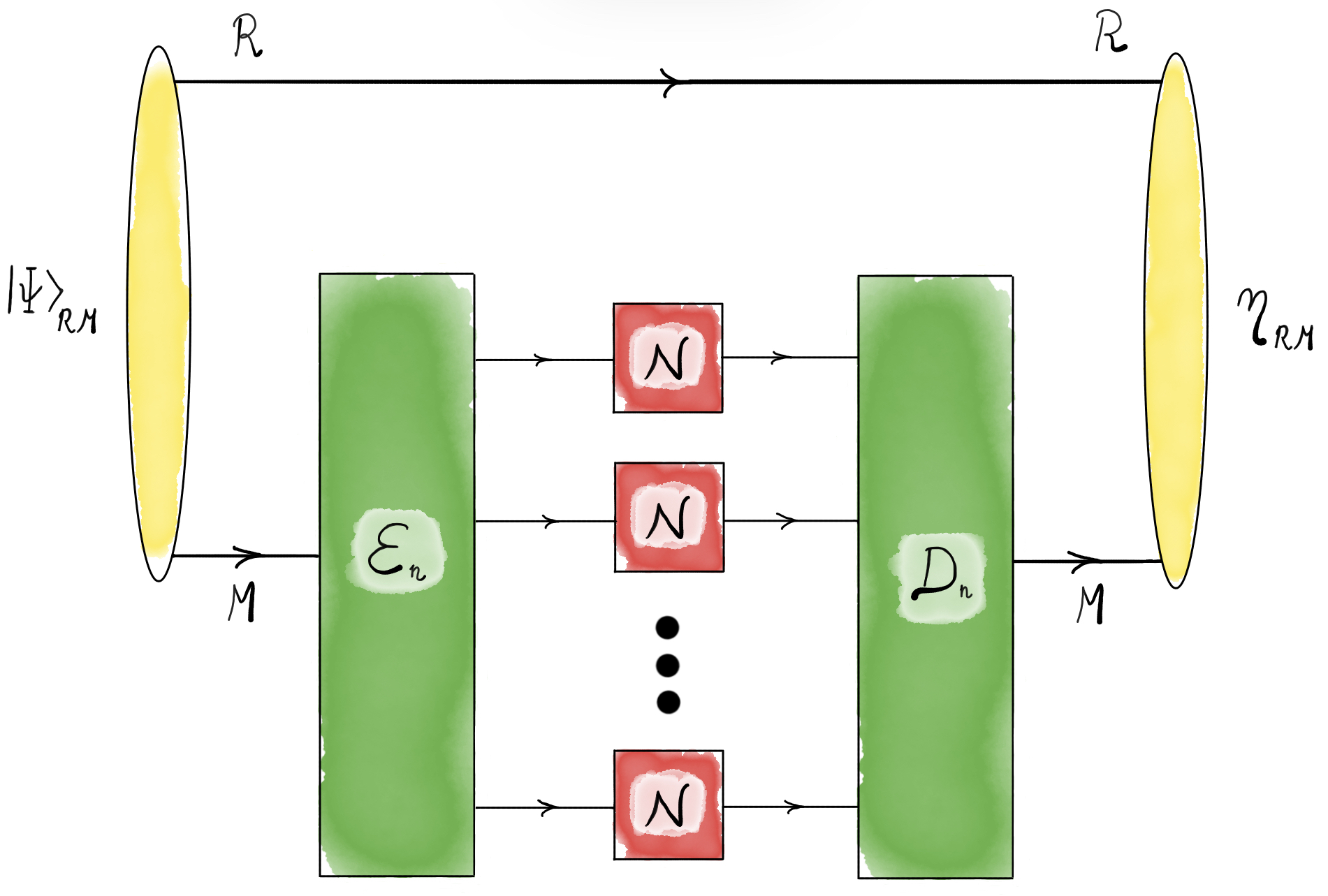
The one-shot quantum capacity $Q_{\varepsilon}(\mathcal{N}_{A\to B})$ of the channel $\mathcal{N}_{A\to B}$ is defined as

\displaystyle\hskip 0.0ptQ_{\varepsilon}(\mathcal{N})\coloneqq\sup_{\mathcal{E},\mathcal{D}}\{\log_{2}|M|:\exists(|M|,\varepsilon)\text{ quantum communication protocol for }\mathcal{N}_{A\to B}\},

(S19)

where the optimization is over every encoding channel $\mathcal{E}$ and decoding channel $\mathcal{D}$ . The (asymptotic) quantum capacity of $\mathcal{N}_{A\to B}$ is then defined as

\displaystyle\hskip 0.0ptQ(\mathcal{N})\coloneqq\inf_{\varepsilon\in(0,1)}\liminf_{n\to\infty}\frac{1}{n}Q_{\varepsilon}(\mathcal{N}^{\otimes n}),

(S20)

where $\mathcal{N}^{\otimes n}$ denotes $n$ copies of the channel $\mathcal{N}$ used in parallel. The strong converse quantum capacity of $\mathcal{N}_{A\to B}$ is defined as

\displaystyle\hskip 0.0ptQ^{\dagger}(\mathcal{N})\coloneqq\sup_{\varepsilon\in(0,1)}\limsup_{n\to\infty}\frac{1}{n}Q_{\varepsilon}(\mathcal{N}^{\otimes n}).

(S21)

The above way of defining quantum capacity is standard, by now, in several references on quantum information theory [24], [79, Section VIII], following the same approach for defining various other capacities in classical and quantum information theory [80, Eqs. (1.6)–(1.7)], [81, Section V-A], [82, Eq. (1)], [83, Eq. (10)]. There are several different ways of defining quantum capacity (see also [84]), but it is known that they lead to the same quantity in the asymptotic limit [85].

It is a classic result of quantum information theory that the quantum capacity is equal to the regularized coherent information of the channel [86, 87, 88, 89, 90, 42]:

	$\displaystyle\hskip 0.0ptQ(\mathcal{N})=$	$\displaystyle\lim_{n\to\infty}\frac{1}{n}\,Q^{(1)}\!\left(\mathcal{N}^{\otimes n}\right)=\sup_{n\in\mathds{N}_{+}}\frac{1}{n}\,Q^{(1)}\!\left(\mathcal{N}^{\otimes n}\right),$		(S22)
	$\displaystyle Q^{(1)}\left(\mathcal{N}\right)\coloneqq$	$\displaystyle\sup_{\ket{\Psi}_{AA^{\prime}}}I_{\mathrm{coh}}(A\rangle B)_{\nu}\,,$		(S22)

where

	$\displaystyle\hskip 0.0pt\nu_{AB}$	$\displaystyle\coloneqq\big(\operatorname{id}_{A}\,\otimes\,\mathcal{N}_{A^{\prime}\to B}\big)(\Psi_{AA^{\prime}}),$		(S23)
	$\displaystyle I_{\mathrm{coh}}(A\rangle B)_{\rho}$	$\displaystyle\coloneqq S(\rho_{B})-S(\rho_{AB})\,.$		(S23)

This gives us a method for evaluating the quantum capacity of particular channels of interest, including the bosonic dephasing channels.

Let us now recall basic definitions related to private capacity. Let $\mathcal{U}^{\mathcal{N}}_{A\to BE}$ be an isometric channel extending the channel $\mathcal{N}_{A\to B}$ [68]. An $(|M|,\varepsilon)$ code for private communication over the channel $\mathcal{N}_{A\to B}$ consists of a set $\{\rho^{m}_{A}\}_{m}$ of encoding states and a decoder, specified as a positive operator-valued measure (POVM) $\{\Lambda^{m}_{B}\}_{m}$ . It achieves an error $\varepsilon$ if there exists a state $\sigma_{E}$ of the environment, such that the following inequality holds for every message $m$ :

\displaystyle\hskip 0.0ptF\left(\sum_{m^{\prime}}\ket{m^{\prime}}\!\!\bra{m^{\prime}}\otimes\Tr_{B}[\Lambda^{m^{\prime}}_{B}\mathcal{U}^{\mathcal{N}}_{A\to BE}(\rho^{m}_{A})],\ket{m}\!\!\bra{m}\otimes\sigma_{E}\right)\geq 1-\varepsilon.

(S24)

The one-shot private capacity $P_{\varepsilon}(\mathcal{N}_{A\to B})$ of the channel $\mathcal{N}_{A\to B}$ is defined as

\displaystyle\hskip 0.0ptP_{\varepsilon}(\mathcal{N})\coloneqq\sup_{\{\rho^{m}_{A}\}_{m},\{\Lambda^{m}_{B}\}_{m}}\{\log_{2}|M|:\exists(|M|,\varepsilon)\text{ private communication protocol for }\mathcal{N}_{A\to B}\},

(S25)

where the optimization is over every set $\{\rho^{m}_{A}\}_{m}$ of encoding states and decoding POVM $\{\Lambda^{m}_{B}\}_{m}$ . The (asymptotic) private capacity of $\mathcal{N}_{A\to B}$ is then defined as

\displaystyle\hskip 0.0ptP(\mathcal{N})\coloneqq\inf_{\varepsilon\in(0,1)}\liminf_{n\to\infty}\frac{1}{n}P_{\varepsilon}(\mathcal{N}^{\otimes n}).

(S26)

The strong converse private capacity of $\mathcal{N}_{A\to B}$ is defined as

\displaystyle\hskip 0.0ptP^{\dagger}(\mathcal{N})\coloneqq\sup_{\varepsilon\in(0,1)}\limsup_{n\to\infty}\frac{1}{n}P_{\varepsilon}(\mathcal{N}^{\otimes n}).

(S27)

The following inequalities are direct consequences of the definitions:

	$\displaystyle\hskip 0.0ptQ(\mathcal{N})$	$\displaystyle\leq Q^{\dagger}(\mathcal{N}),$		(S28)
	$\displaystyle P(\mathcal{N})$	$\displaystyle\leq P^{\dagger}(\mathcal{N}).$		(S28)

Less trivially, we also have that [42]

\displaystyle\hskip 0.0ptQ(\mathcal{N})

\displaystyle\leq P(\mathcal{N}).

(S29)

II.5 Two-way assisted capacities of quantum channels

In this section, we define the quantum and private capacities when the channel of interest is assisted by local operations and classical communication (LOCC). We begin with the LOCC-assisted quantum capacity.

An $(n,|M|,\varepsilon)$ protocol $\mathcal{P}$ for LOCC-assisted quantum communication consists of a separable state $\sigma_{A^{\prime}_{1}A_{1}B^{\prime}_{1}}$ (which is understood to be separable with respect to the bipartition $A^{\prime}_{1}A_{1}:B^{\prime}_{1}$ ), the set $\big\{\mathcal{L}^{(i-1)}_{A^{\prime}_{i-1}B_{i-1}B^{\prime}_{i-1}\to A^{\prime}_{i}A_{i}B^{\prime}_{i}}\big\}_{i=2}^{n}$ of LOCC channels, and the LOCC channel $\mathcal{L}^{(n)}_{A^{\prime}_{n}B_{n}B^{\prime}_{n}\to M_{A}M_{B}}$ . (See [91] for the definition of an LOCC channel.) We can also imagine that the state $\sigma_{A^{\prime}_{1}A_{1}B^{\prime}_{1}}$ is produced by an LOCC preprocessing channel $\mathcal{L}^{(0)}_{A^{\prime}_{0}B^{\prime}_{0}\to A^{\prime}_{1}A_{1}B^{\prime}_{1}}$ , with the $A^{\prime}_{0}B^{\prime}_{0}$ system initialised in a product state. The final state of the protocol is

	$\displaystyle\hskip 0.0pt\eta_{M_{A}M_{B}}\coloneqq\Big(\mathcal{L}^{(n)}_{A^{\prime}_{n}B_{n}B^{\prime}_{n}\to M_{A}M_{B}}\circ\mathcal{N}_{A_{n}\to B_{n}}$	$\displaystyle\circ\mathcal{L}^{(n-1)}_{A^{\prime}_{n-1}B_{n-1}B^{\prime}_{n-1}\to A^{\prime}_{n}A_{n}B^{\prime}_{n}}\circ\cdots$		(S30)
		$\displaystyle\circ\mathcal{L}^{(1)}_{A^{\prime}_{1}B_{1}B^{\prime}_{1}\to A^{\prime}_{2}A_{2}B^{\prime}_{2}}\circ\mathcal{N}_{A_{1}\to B_{1}}\Big)\big(\sigma_{A^{\prime}_{1}A_{1}B^{\prime}_{1}}\big)\,,$		(S30)

satisfying

\displaystyle\hskip 0.0ptF(\eta_{M_{A}M_{B}},\Phi_{M_{A}M_{B}})\geq 1-\varepsilon,

(S31)

where $\Phi_{M_{A}M_{B}}$ is a maximally entangled state of Schmidt rank $|M|$ . Such a protocol is depicted in Figure S5. We note here that it suffices for such a protocol to generate the maximally entangled state $\Phi_{M_{A}M_{B}}$ because entanglement and quantum communication are equivalent communication resources when classical communication is freely available, due to the teleportation protocol [92].

The $n$ -shot LOCC-assisted quantum capacity of the channel $\mathcal{N}_{A\to B}$ is defined as

\displaystyle\hskip 0.0ptQ_{\leftrightarrow,n,\varepsilon}(\mathcal{N})\coloneqq\sup_{\mathcal{P}}\left\{\frac{1}{n}\log_{2}|M|:\exists(n,|M|,\varepsilon)\text{ LOCC-assisted q.~comm.~protocol }\mathcal{P}\text{ for }\mathcal{N}_{A\to B}\right\},

(S32)

where the optimization is over every LOCC-assisted quantum communication protocol $\mathcal{P}$ . The (asymptotic) LOCC-assisted quantum capacity of $\mathcal{N}_{A\to B}$ is then defined as

\displaystyle\hskip 0.0ptQ_{\leftrightarrow}(\mathcal{N})\coloneqq\inf_{\varepsilon\in(0,1)}\liminf_{n\to\infty}Q_{\leftrightarrow,n,\varepsilon}(\mathcal{N}).

(S33)

The strong converse LOCC-assisted quantum capacity of $\mathcal{N}_{A\to B}$ is defined as

\displaystyle\hskip 0.0ptQ^{\dagger}_{\leftrightarrow}(\mathcal{N})\coloneqq\sup_{\varepsilon\in(0,1)}\limsup_{n\to\infty}Q_{\leftrightarrow,n,\varepsilon}(\mathcal{N}).

(S34)

An $(n,|M|,\varepsilon)$ protocol $\mathcal{K}$ for secret key agreement over a quantum channel is defined essentially the same as an LOCC-assisted protocol for quantum communication, except that the target final state of the protocol is more general. That is, the final step of the protocol is an LOCC channel $\mathcal{L}^{(n)}_{A^{\prime}_{n}B_{n}B^{\prime}_{n}\to M_{A}M_{B}S_{A}S_{B}}$ , where $S_{A}$ and $S_{B}$ are extra systems of the sender Alice and the receiver Bob. Let us then denote the final state of the protocol by $\eta_{M_{A}M_{B}S_{A}S_{B}}$ . Such a protocol satisfies

\displaystyle\hskip 0.0ptF(\eta_{M_{A}M_{B}S_{A}S_{B}},\gamma_{M_{A}M_{B}S_{A}S_{B}})\geq 1-\varepsilon,

(S35)

where $\gamma_{M_{A}M_{B}S_{A}S_{B}}$ is a private state of dimension $|M|$ [61, 62], having the form

\displaystyle\hskip 0.0pt\gamma_{M_{A}M_{B}S_{A}S_{B}}\coloneqq U_{M_{A}M_{B}S_{A}S_{B}}(\Phi_{M_{A}M_{B}}\otimes\theta_{S_{A}S_{B}})U_{M_{A}M_{B}S_{A}S_{B}}^{\dagger}.

(S36)

In the above, $U_{M_{A}M_{B}S_{A}S_{B}}$ is a twisting unitary of the form

\displaystyle\hskip 0.0ptU_{M_{A}M_{B}S_{A}S_{B}}=\sum_{i,j}\ket{i}\!\!\bra{i}_{M_{A}}\otimes\ket{j}\!\!\bra{j}_{M_{B}}\otimes U^{i,j}_{S_{A}S_{B}},

(S37)

with each $U^{i,j}_{S_{A}S_{B}}$ a unitary. Also, $\Phi_{M_{A}M_{B}}$ is a maximally entangled state of Schmidt rank $|M|$ and $\theta_{S_{A}S_{B}}$ is an arbitrary state. The fact that such a protocol is equivalent to the more familiar notion of secret key agreement, involving three parties generating a tripartite secret key state of the form $\frac{1}{|M|}\sum_{m=0}^{|M|-1}\ket{m}\!\!\bra{m}_{M_{A}}\otimes\ket{m}\!\!\bra{m}_{M_{B}}\otimes\sigma_{E}$ , is the main contribution of [61, 62] (see [24] for another presentation).

The $n$ -shot secret-key-agreement capacity of the channel $\mathcal{N}_{A\to B}$ is defined as

\displaystyle\hskip 0.0ptP_{\!\leftrightarrow,n,\varepsilon}(\mathcal{N})\coloneqq\sup_{\mathcal{K}}\left\{\frac{1}{n}\log_{2}|M|:\exists(n,|M|,\varepsilon)\text{ secret-key-agreement protocol }\mathcal{K}\text{ for }\mathcal{N}_{A\to B}\right\},

(S38)

where the optimization is over every secret key agreement protocol $\mathcal{K}$ . The (asymptotic) secret key agreement capacity of $\mathcal{N}_{A\to B}$ is then defined as

\displaystyle\hskip 0.0ptP_{\!\leftrightarrow}(\mathcal{N})\coloneqq\inf_{\varepsilon\in(0,1)}\liminf_{n\to\infty}P_{\!\leftrightarrow,n,\varepsilon}(\mathcal{N}).

(S39)

The strong converse secret key agreement capacity of $\mathcal{N}_{A\to B}$ is defined as

\displaystyle\hskip 0.0ptP^{\dagger}_{\!\leftrightarrow}(\mathcal{N})\coloneqq\sup_{\varepsilon\in(0,1)}\limsup_{n\to\infty}P_{\!\leftrightarrow,n,\varepsilon}(\mathcal{N}).

(S40)

The following inequalities are direct consequences of the definitions:

	$\displaystyle\hskip 0.0ptQ_{\leftrightarrow}(\mathcal{N})$	$\displaystyle\leq Q_{\leftrightarrow}^{\dagger}(\mathcal{N})$		(S41)
	$\displaystyle P_{\!\leftrightarrow}(\mathcal{N})$	$\displaystyle\leq P_{\!\leftrightarrow}^{\dagger}(\mathcal{N}).$		(S41)

Due to the fact that a more general target state is allowed in secret key agreement, the following inequalities hold

	$\displaystyle\hskip 0.0ptQ_{\leftrightarrow}(\mathcal{N})$	$\displaystyle\leq P_{\!\leftrightarrow}(\mathcal{N})$		(S42)
	$\displaystyle Q^{{\dagger}}_{\leftrightarrow}(\mathcal{N})$	$\displaystyle\leq P^{{\dagger}}_{\leftrightarrow}(\mathcal{N}).$		(S42)

Finally, due to the fact that classical communication can only enhance capacities, the following inequalities hold:

$\displaystyle\hskip 0.0ptQ(\mathcal{N})$	$\displaystyle\leq Q_{\leftrightarrow}(\mathcal{N})$	(S43)
$\displaystyle Q^{{\dagger}}(\mathcal{N})$	$\displaystyle\leq Q^{{\dagger}}_{\leftrightarrow}(\mathcal{N})$
$\displaystyle P(\mathcal{N})$	$\displaystyle\leq P_{\!\leftrightarrow}(\mathcal{N})$
$\displaystyle P^{{\dagger}}(\mathcal{N})$	$\displaystyle\leq P^{{\dagger}}_{\leftrightarrow}(\mathcal{N}).$

Thus, to establish the collapse of all of the capacities discussed in this section and the previous one, for the case of bosonic dephasing channels, it suffices to prove the lower bound on $Q(\mathcal{N})$ and the upper bound on $P^{{\dagger}}_{\leftrightarrow}(\mathcal{N})$ .

II.6 Teleportation simulation

The $d$ -dimensional quantum teleportation protocol [92] takes as input a $d$ -dimensional quantum state $\rho_{A^{\prime}}$ of a system $A^{\prime}$ , a $d$ -dimensional maximally entangled state

\displaystyle\hskip 0.0pt\Phi_{d}^{AB}\coloneqq\ket{\Phi_{d}}\!\!\bra{\Phi_{d}}_{AB}\,,\qquad\ket{\Phi_{d}}_{AB}\coloneqq\frac{1}{\sqrt{d}}\sum_{k=0}^{d-1}\ket{k}_{A}\ket{k}_{B}\,,

(S44)

and by using only local operations and one-way classical communication from Alice to Bob reproduces the exact same state $\rho$ on the system $B$ . To define it rigorously, for $x,z\in\{0,\ldots,d-1\}$ let us introduce the unitary matrices

\displaystyle\hskip 0.0ptX(x)\,\coloneqq\,\sum_{k=0}^{d-1}\ket{k\oplus x}\!\!\bra{k}\,,\qquad Z(z)\,\coloneqq\,\sum_{k=0}^{d-1}e^{\frac{2\pi i}{d}zk}\ket{k}\!\!\bra{k}\,,\qquad U(x,z)\coloneqq X(x)Z(z)\,,

(S45)

where $\oplus$ denotes sum modulo $d$ . Then the teleportation channel $\pazocal{T}^{(d)}_{A^{\prime}AB\to B}$ is given by

\displaystyle\hskip 0.0pt\pazocal{T}^{(d)}_{A^{\prime}AB\to B}(X_{A^{\prime}AB})\coloneqq\sum_{x,z=0}^{d-1}U(x,z)_{B}\Tr_{AA^{\prime}}\!\left[X_{A^{\prime}AB}\,U(x,z)_{A^{\prime}}\Phi_{d}^{AA^{\prime}}U(x,z)_{A^{\prime}}^{\dagger}\right]U(x,z)_{B}^{{\dagger}}\,.

(S46)

The effectiveness of the standard quantum teleportation protocol is expressed by the identity

\displaystyle\hskip 0.0pt\pazocal{T}^{(d)}_{A^{\prime}AB\to B}\!\left(\rho_{A^{\prime}}\otimes\Phi_{d}^{AB}\right)=\rho_{B}\,,

(S47)

meaning that the same operator $\rho$ is written in the registers $A^{\prime}$ and $B$ on the left-hand and on the right-hand side, respectively.

Some channels can be simulated by the action of the standard teleportation protocol on their Choi states [22], in the sense that

\displaystyle\hskip 0.0pt\pazocal{T}^{(d)}_{A^{\prime}AB\to B}\!\left(\rho_{A^{\prime}}\otimes\Phi_{\mathcal{N}}^{AB}\right)=\mathcal{N}(\rho_{A^{\prime}})\,,

(S48)

where $\Phi_{\mathcal{N}}^{AB}$ is the Choi state of the channel $\mathcal{N}$ . For example, this is the case for all Pauli channels. More generally, other channels can be simulated approximately by the action of the teleportation protocol on their Choi states. This concept was introduced in [22] for the explicit purpose of obtaining upper bounds on the LOCC-assisted quantum capacity of a channel in terms of an entanglement measure evaluated on the Choi state. The idea was rediscovered in [93] for the same purpose, and more recently the same idea was used to bound the secret-key-agreement capacity [36] and the strong converse secret-key-agreement capacity [25]. Here we make use of this concept in order to obtain upper bounds on the strong converse secret key agreement capacity of all bosonic dephasing channels. As discussed earlier, it suffices to consider establishing an upper bound on this latter capacity because it is the largest among all the capacities that we consider in this paper.

II.7 Bosonic dephasing channel

Definition S2.

Let $p$ be a probability density function on the interval $[-\pi,\pi]$ . The associated bosonic dephasing channel is the quantum channel $\mathcal{N}_{p}:\pazocal{T}(\pazocal{H}_{1})\to\pazocal{T}(\pazocal{H}_{1})$ acting on a single-mode system and given by

\displaystyle\hskip 0.0pt\mathcal{N}_{p}(\rho)\coloneqq\int_{-\pi}^{\pi}d\phi\ p(\phi)\,e^{-ia^{\dagger}\!a\,\phi}\rho\,e^{ia^{\dagger}\!a\,\phi}\,,

(S49)

where $a^{\dagger}a$ is the photon number operator.

The action of the bosonic dephasing channel can be easily described by representing the input operator in the Fock basis. By means of this representation the Hilbert space of a single-mode system, $\pazocal{H}_{1}$ , becomes equivalent to that of square-summable complex-valued sequences, denoted $\ell^{2}(\mathds{N})$ . Operators on $\pazocal{H}_{1}$ are represented by infinite matrices, i.e., operators $S:\ell^{2}(\mathds{N})\to\ell^{2}(\mathds{N})$ . Given two such operators $S,T$ , which we formally write $S=\sum_{h,k}S_{hk}\ket{h}\!\!\bra{k}$ and $T=\sum_{h,k}T_{hk}\ket{h}\!\!\bra{k}$ , their Hadamard product is defined by

\displaystyle\hskip 0.0ptS\circ T\coloneqq\sum_{h,k}S_{hk}T_{hk}\ket{h}\!\!\bra{k}\,.

(S50)

One of the fundamental facts concerning the Hadamard product is the Schur product theorem [94, Theorem 7.5.3]: it states that if $S\geq 0$ and $T\geq 0$ are positive semi-definite, then also $S\circ T\geq 0$ is such. The theorem is usually stated for matrices, but is is immediately generalisable to the operator case as a consequence of the remark below.

Remark S3.

Let $T:\ell^{2}(\mathds{N})\to\ell^{2}(\mathds{N})$ be an infinite matrix. Then $T\geq 0$ if and only if $T^{(d)}\geq 0$ for all $d\in\mathds{N}_{+}$ , where $T^{(d)}$ is the $d\times d$ top left corner of $T$ . This follows from the fact that the linear span of the basis vectors $\ket{k}$ , $k\in\mathds{N}$ , is dense in $\ell^{2}(\mathds{N})$ .

Given an infinite matrix $T$ which represents a bounded operator $T:\ell^{2}(\mathds{N})\to\ell^{2}(\mathds{N})$ , we can define the associated Hadamard channel as

\displaystyle\hskip 0.0pt\begin{array}[]{ccccc}\mathcal{L}_{T}&:&\pazocal{T}\left(\ell^{2}(\mathds{N})\right)&\longrightarrow&\pazocal{T}\left(\ell^{2}(\mathds{N})\right)\\[4.30554pt] &&S&\longmapsto&S\circ T\,.\end{array}

(S51)

When restricted to finite-dimensional systems, Hadamard channels are examples of so-called ‘partially coherent direct sum channels’ [95]. The following is then easily established.

Lemma S4.

Let $T:\ell^{2}(\mathds{N})\to\ell^{2}(\mathds{N})$ be a bounded operator represented by an infinite matrix. Then the Hadamard channel $\mathcal{L}_{T}$ defined by (S51) is a completely positive and trace preserving map, i.e., a quantum channel, if and only if

(i)

$T\geq 0$ as an operator; and
(ii)

$T_{kk}=1$ for all $k\in\mathds{N}$ .

Proof.

The two conditions are clearly necessary. In fact, if $T_{kk}\neq 1$ for some $k\in\mathds{N}_{+}$ , then $\Tr[T\circ\ket{k}\!\!\bra{k}]=T_{kk}\neq 1=\Tr\ket{k}\!\!\bra{k}$ ; i.e., $\mathcal{L}_{T}$ is not trace preserving. Also, if $T\ngeq 0$ then by Remark S3 there exists $d\in\mathds{N}_{+}$ and some $\ket{\psi}\in\mathds{C}^{d}$ such that $\braket{\psi|T^{(d)}|\psi}<0$ . Rewriting $\braket{\psi|T^{(d)}|\psi}=\sum_{h,k=0}^{d-1}\psi_{h}^{*}\psi_{k}T_{hk}=d\braket{+|(T\circ\psi)|+}$ , where $\psi\coloneqq\ket{\psi}\!\!\bra{\psi}$ and $\ket{+}\coloneqq\frac{1}{\sqrt{d}}\sum_{k=0}^{d-1}\ket{k}$ , shows that in this case $\mathcal{L}_{T}$ would not even be positive, let alone completely positive.

Vice versa, conditions (i)–(ii) are sufficient. In fact, on the one hand, by (ii), for an arbitrary $X$ , we have that $\Tr\mathcal{L}_{T}(X)=\sum_{k}T_{kk}X_{kk}=\Tr X$ , i.e., $\mathcal{L}_{T}$ is trace preserving. On the other hand, if $T\geq 0$ then for all $d\in\mathds{N}_{+}$ and for all positive semi-definite bipartite operators $X\geq 0$ acting on $\mathds{C}^{d}\otimes\ell^{2}(\mathds{N})$ we have that $\left(I\otimes\mathcal{L}_{T}\right)(X)=d\left(\ket{+}\!\!\bra{+}\otimes T\right)\circ X\geq 0$ , where $\ket{+}$ is defined above, and the last inequality follows by the Schur product theorem. Since $d$ is arbitrary, this proves that $\mathcal{L}_{T}$ is completely positive. ∎

The theory of Hadamard channels we just sketched out is relevant here due to the following simple observation.

Lemma S5.

When both the input and the output density operators are represented in the Fock basis, the bosonic dephasing channel $\mathcal{N}_{p}$ acts as the Hadamard channel

	$\displaystyle\mathcal{N}_{p}(\rho)=$	$\displaystyle\ \rho\circ T_{p}\,,$		(S52)
	$\displaystyle(T_{p})_{hk}\coloneqq$	$\displaystyle\ \int_{-\pi}^{\pi}d\phi\ p(\phi)\,e^{-i\phi(h-k)}\,.$		(S53)

Proof.

Due to (S16), we have that $\mathcal{N}_{p}(\rho)=\sum_{h,k}\rho_{hk}\int_{-\pi}^{\pi}d\phi\ p(\phi)\,e^{-i\phi(h-k)}\ket{h}\!\!\bra{k}=\rho\circ T_{p}$ . ∎

III Capacities of bosonic dephasing channels

III.1 Infinite Toeplitz matrices and theorems of Szegő and Avram–Parter type

Observe that the expression for $(T_{p})_{hk}$ only depends on the difference $h-k$ . Matrices with this property are named after the mathematician Otto Toeplitz. Formally, a Toeplitz matrix of size $d\in\mathds{N}_{+}$ is a matrix of the form

\displaystyle\hskip 0.0ptT=\begin{pmatrix}a_{0}&a_{-1}&a_{-2}&\ldots&a_{-d+1}\\ a_{1}&a_{0}&a_{-1}&\ldots&a_{-d+2}\\ a_{2}&a_{1}&a_{0}&\ldots&a_{-d+3}\\ \vdots&\vdots&\vdots&\ddots&\vdots\\ a_{d-1}&a_{d-2}&a_{d-3}&\ldots&a_{0}\end{pmatrix},

(S54)

where $a_{0},\ldots,a_{d-1}\in\mathds{C}$ . Alternatively, it can be defined to have entries

\displaystyle\hskip 0.0ptT_{hk}=a_{h-k}\,.

(S55)

This definition can be formally extended to the case of infinite Toeplitz matrices, simply by letting $h,k\in\mathds{N}$ run over all non-negative integers. Note that the top left corners $T^{(d)}\coloneqq\sum_{h,k=0}^{d-1}T_{hk}\ket{h}\!\!\bra{k}$ of an infinite Toeplitz matrix are Toeplitz matrices themselves.

In applications one often encounters the case in which the numbers $a_{k}$ are the Fourier coefficients of an absolutely integrable function $a:[-\pi,\pi]\to\mathds{C}$ , i.e.

\displaystyle\hskip 0.0pta_{k}=\int_{-\pi}^{+\pi}\frac{d\phi}{2\pi}\ a(\phi)\,e^{-ik\phi}.

(S56)

In this paper, we will consider mainly non-negative functions $a:[-\pi,\pi]\to\mathds{R}_{+}$ .

A result due to Szegő [47, 96] states that the spectrum of the $d\times d$ top left corners $T^{(d)}$ of an infinite Toeplitz matrix converges to the generating function $a:[-\pi,\pi]\to\mathds{R}$ (for now assumed to be real-valued), in the sense that

\displaystyle\hskip 0.0pt\lim_{d\to\infty}\frac{1}{d}\Tr F\big(T^{(d)}\big)=\lim_{d\to\infty}\frac{1}{d}\sum_{j=1}^{d}F\big(\lambda_{j}\big(T^{(d)}\big)\big)=\int_{-\pi}^{\pi}\frac{d\phi}{2\pi}\ F\big(a(\phi)\big)

(S57)

whenever $a$ and $F:\mathds{R}\to\mathds{R}$ are sufficiently well behaved. Here, $\lambda_{j}\big(T^{(d)}\big)$ denotes the $j^{\text{th}}$ eigenvalue of the matrix $T^{(d)}$ . The scope and extension of Szegő’s result has been expanded over the years by relaxing the conditions to be imposed on $a$ and $F$ so that (S57) holds. At the same time, an analogous class of results, initially conceived by Parter [97] and Avram [98], has been developed to deal with the case of complex-valued generating functions $a:[-\pi,\pi]\to\mathds{C}$ . Results of the Avram–Parter type generalize (S57) by stating that

\displaystyle\hskip 0.0pt\lim_{d\to\infty}\frac{1}{d}\Tr F\Big(\big|T^{(d)}\big|\Big)=\lim_{d\to\infty}\frac{1}{d}\sum_{j=1}^{d}F\big(s_{j}\big(T^{(d)}\big)\big)=\int_{-\pi}^{\pi}\frac{d\phi}{2\pi}\ F\Big(\big|a(\phi)\big|\Big)\,,

(S58)

where $s_{j}\big(T^{(d)}\big)$ is now the $j^{\text{th}}$ singular value of the matrix $T^{(d)}$ . Both Szegő’s and Avram–Parter’s result have been generalized in successive steps, by Zamarashkin and Tyrtyshnikov [99], Tilli [100], Serra-Capizzano [48], Böttcher, Grudsky, and Maksimenko [101], and others. For a detailed account of these developments, we refer the reader to the textbooks [102, 103, 104] and especially to the lecture notes by Grudsky [105]. Here we will just need the following lemma, extracted from the work of Serra-Capizzano.

Lemma S6 ((Serra-Capizzano [48])).

If $a:[-\pi,\pi]\to\mathds{R}_{+}$ is such that

\displaystyle\hskip 0.0pt\int_{-\pi}^{+\pi}\frac{d\phi}{2\pi}\ a(\phi)^{\alpha}<\infty

(S59)

for some $\alpha\geq 1$ , and moreover $F:\mathds{R}_{+}\to\mathds{R}$ is continuous and satisfies

\displaystyle\hskip 0.0ptF(x)=O(x^{\alpha})\qquad(x\to\infty)\,,

(S60)

then (S57) holds.

Proof.

The original result by Serra-Capizzano [48, Theorem 2] states that the identity (S58) involving singular values holds. However, under the stronger hypotheses that we are making here it can be seen that (S57) and (S58) are actually equivalent. Since $a$ takes on values in $\mathds{R}_{+}$ , we only need to check that for each $d$ the singular values and the eigenvalues of $T^{(d)}$ coincide. To this end, it suffices to note that $T^{(d)}$ is a positive semi-definite operator, simply because

$\displaystyle\hskip 0.0pt\sum_{h,k=0}^{d-1}\psi_{h}^{*}\psi_{k}T_{hk}$	$\displaystyle=\sum_{h,k=0}^{d-1}\psi_{h}^{*}\psi_{k}\int_{-\pi}^{+\pi}\frac{d\phi}{2\pi}\ a(\phi)\,e^{-i(h-k)\phi}$	(S61)
	$\displaystyle=\int_{-\pi}^{+\pi}\frac{d\phi}{2\pi}\ a(\phi)\sum_{h,k=0}^{d-1}\psi_{h}^{*}\psi_{k}\,e^{-i(h-k)\phi}$
	$\displaystyle=\int_{-\pi}^{+\pi}\frac{d\phi}{2\pi}\ a(\phi)\left\|\sum\nolimits_{k=0}^{d-1}\psi_{k}\,e^{ik\phi}\right\|^{2}$
	$\displaystyle\geq 0$

for every $\ket{\psi}\in\mathds{C}^{d}$ . This can also be seen as a simple consequence of (the easy direction of) Bochner’s theorem. ∎

III.2 Proof of main result

Before stating and proving our main result, let us fix some terminology. For an infinite matrix $\tau$ that is also a density operator on $\ell^{2}(\mathds{N})$ , the associated maximally correlated state $\Omega[\tau]$ on $\ell^{2}(\mathds{N})\otimes\ell^{2}(\mathds{N})$ is defined by

\displaystyle\hskip 0.0pt\Omega[\tau]\coloneqq\sum_{h,k=0}^{\infty}\tau_{hk}\ket{h}\!\!\bra{k}\otimes\ket{h}\!\!\bra{k}\,.

(S62)

Maximally correlated states appear naturally in connecting coherence theory [106, 107, 108, 109, 110, 111, 112, 113, 114] (see also the review article [115]) with entanglement theory. When seen in this latter context, they are useful because they represent a particularly simple class of entangled states.

Before we proceed further, let us recall in passing that the Rényi entropy of a probability density defined on the interval $[-\pi,\pi]$ need not be finite; that is, it can be equal to $-\infty$ . It is always bounded from above by $\log_{2}(2\pi)$ , due to the non-negativity of relative entropy. Indeed, $h_{\alpha}(p)\leq\log_{2}(2\pi)$ for every probability density $p$ defined on $[-\pi,\pi]$ and for all $\alpha\in(0,1)\cup(1,\infty)$ , because $\log_{2}(2\pi)-h_{\alpha}(p)=D_{\alpha}(p\|u)\geq 0$ , where $u$ is the uniform probability density on $[-\pi,\pi]$ . The same is true for the case $\alpha=1$ , where we identify $h_{1}$ with the standard differential entropy (S6). However, as an example, if we take the probability density to be $p(x)=c|x|^{-\frac{1}{\alpha}}$ for $\alpha>1$ , where $c$ is a normalization factor, then the Rényi entropy $h_{\alpha}(p)$ diverges to $-\infty$ . Note that the condition $h_{\alpha}(p)>-\infty$ is equivalent to the condition $\int_{-\pi}^{+\pi}d\phi\ p(\phi)^{\alpha}<\infty$ . An analogous reasoning can be repeated for the case where $\alpha=1$ . Here, $p(x)\propto|x|^{-1}\left(\log_{2}\frac{2\pi}{|x|}\right)^{-2}$ provides an example of a probability distribution for which $h(p)=-\infty$ (while $p$ itself is integrable).

Theorem S7.

Let $p:[-\pi,+\pi]\to\mathds{R}_{+}$ be a probability density function with the property that one of its Rényi entropies is finite for some $\alpha_{0}>1$ , i.e.

\displaystyle\hskip 0.0pt\int_{-\pi}^{+\pi}d\phi\ p(\phi)^{\alpha_{0}}<\infty\,.

(S63)

Then the two-way assisted quantum capacity, the unassisted quantum capacity, the private capacity, the secret-key capacity, and all of the corresponding strong converse capacities of the associated bosonic dephasing channel $\mathcal{N}_{p}$ coincide, and are given by the expression

$\displaystyle\hskip 0.0ptQ(\mathcal{N}_{p})$	$\displaystyle=Q^{\dagger}(\mathcal{N}_{p})=P(\mathcal{N}_{p})=P^{\dagger}(\mathcal{N}_{p})=Q_{\leftrightarrow}(\mathcal{N}_{p})=Q_{\leftrightarrow}^{\dagger}(\mathcal{N}_{p})=P(\mathcal{N}_{p})=P_{\!\leftrightarrow}^{\dagger}(\mathcal{N}_{p})$	(S64)
	$\displaystyle=D(p\\|u)=\log_{2}(2\pi)-h(p)$
	$\displaystyle=\log_{2}(2\pi)-\int_{-\pi}^{\pi}d\phi\ p(\phi)\log_{2}\frac{1}{p(\phi)}\,.$

Here, $D(p\|u)$ denotes the Kullback–Leibler divergence between $p$ and the uniform probability density $u$ over $[-\pi,\pi]$ , and $h(p)$ is the differential entropy of $p$ .

Remark S8.

The condition on the Rényi entropy of $p$ is of a purely technical nature. We expect it to be obeyed in all cases of practical interest. For example, it holds true provided that $p$ is bounded on $[-\pi,\pi]$ .

Remark S9.

By using Hölder’s inequality, it can be easily verified that if (S63) holds for $\alpha_{0}\geq 1$ then it holds for all $\alpha$ such that $1\leq\alpha\leq\alpha_{0}$ .

Proof of Theorem S7.

The smallest of all eight quantities is the unassisted quantum capacity $Q(\mathcal{N}_{p})$ , and the largest is $P_{\!\leftrightarrow}^{\dagger}(\mathcal{N}_{p})$ . Therefore, it suffices to prove that

\displaystyle\hskip 0.0ptQ(\mathcal{N}_{p})\geq D(p\|u)\,,\qquad P_{\!\leftrightarrow}^{\dagger}(\mathcal{N}_{p})\leq D(p\|u)\,.

(S65)

Note that it is elementary to verify that

\displaystyle\hskip 0.0ptD(p\|u)=\int_{-\pi}^{+\pi}d\phi\ p(\phi)\log_{2}\frac{p(\phi)}{1/(2\pi)}=\log_{2}(2\pi)-\int_{-\pi}^{+\pi}d\phi\ p(\phi)\log_{2}\frac{1}{p(\phi)}=\log_{2}(2\pi)-h(p)\,,

(S66)

where the differential entropy $h(p)$ is defined by (S6).

To bound $Q(\mathcal{N}_{p})$ from below, we need an ansatz for a state $\ket{\Psi}_{AA^{\prime}}$ to plug into (S22). Letting $A$ and $A^{\prime}$ be single-mode systems, we can consider the maximally entangled state $\ket{\Phi_{d}}_{AA^{\prime}}\coloneqq\frac{1}{\sqrt{d}}\sum_{k=0}^{d-1}\ket{k}_{A}\ket{k}_{A^{\prime}}$ locally supported on the subspace spanned by first $d$ Fock states $\ket{k}$ (see (S15)), where $k\in\{0,\ldots,d-1\}$ . Let us also define the truncated matrix

\displaystyle\hskip 0.0ptT_{p}^{(d)}\coloneqq\Pi_{d}T_{p}\Pi_{d}=\sum_{h,k=0}^{d-1}(T_{p})_{hk}\ket{h}\!\!\bra{k}\,,

(S67)

where

\displaystyle\hskip 0.0pt\Pi_{d}\coloneqq\sum_{k=0}^{d-1}\ket{k}\!\!\bra{k}\,.

(S68)

Then note that

$\displaystyle\hskip 0.0pt\omega_{p,d}\coloneqq$	$\displaystyle\big(I\otimes\mathcal{N}_{p}\big)\big(\Phi_{d}\big)$	(S69)
$\displaystyle=$	$\displaystyle\frac{1}{d}\sum_{h,k=0}^{d-1}\big(I\,\otimes\,\mathcal{N}_{p}\big)\big(\ket{hh}\!\!\bra{kk}\big)$
$\displaystyle=$	$\displaystyle\frac{1}{d}\sum_{h,k=0}^{d-1}(T_{p})_{hk}\ket{hh}\!\!\bra{kk}$
$\displaystyle=$	$\displaystyle\frac{1}{d}\,\Omega\big[T_{p}^{(d)}\big]\,,$

where $\Omega[\tau]$ is defined by (S62). Consider that

$\displaystyle Q(\mathcal{N}_{p})$	$\displaystyle\stackrel{{\scriptstyle\mathclap{\scriptsize\mbox{(i)}}}}{{\geq}}\limsup_{d\to\infty}I_{\mathrm{coh}}(A\rangle B)_{\big(I\,\otimes\,\mathcal{N}_{p}^{A^{\prime}\to B}\big)\big(\Phi_{d}^{AA^{\prime}}\big)}$
	$\displaystyle\stackrel{{\scriptstyle\mathclap{\scriptsize\mbox{(ii)}}}}{{=}}\limsup_{d\to\infty}I_{\mathrm{coh}}(A\rangle B)_{\omega_{p,d}}$
	$\displaystyle\stackrel{{\scriptstyle\mathclap{\scriptsize\mbox{(iii)}}}}{{=}}\limsup_{d\to\infty}\left(\log_{2}d-S\left(T_{p}^{(d)}\big/d\right)\right)$
	$\displaystyle\stackrel{{\scriptstyle\mathclap{\scriptsize\mbox{(iv)}}}}{{=}}\limsup_{d\to\infty}\left(\log_{2}d+\frac{1}{d}\Tr T_{p}^{(d)}\!\left(-\log_{2}d+\log_{2}T_{p}^{(d)}\right)\right)$	(S70)
	$\displaystyle=\limsup_{d\to\infty}\frac{1}{d}\Tr T_{p}^{(d)}\log_{2}T_{p}^{(d)}$
	$\displaystyle\stackrel{{\scriptstyle\mathclap{\scriptsize\mbox{(v)}}}}{{=}}\int_{-\pi}^{\pi}\frac{d\phi}{2\pi}\ \left(2\pi p(\phi)\right)\log_{2}\left(2\pi p(\phi)\right)$
	$\displaystyle=\log_{2}(2\pi)-\int_{-\pi}^{\pi}d\phi\ p(\phi)\log_{2}\frac{1}{p(\phi)}\,.$

Here: (i) follows from the LSD theorem (S22); in (ii) we introduced the state $\omega_{p,d}$ defined by (S62); (iii) comes from (S23), due to the fact that $S(\Omega[\tau])=S(\tau)$ on the one hand, and

$\displaystyle\Tr_{A}\omega_{p,d}^{AB}$	$\displaystyle=\Tr_{A}\big(I\otimes\mathcal{N}_{p}^{A^{\prime}\to B}\big)\big(\Phi_{d}^{AA^{\prime}}\big)$
	$\displaystyle=\frac{1}{d}\Tr_{A}\!\sum_{h,k=0}^{d-1}(T_{p})_{hk}\ket{h}\!\!\bra{k}_{A}\otimes\ket{h}\!\!\bra{k}_{B}$
	$\displaystyle=\frac{1}{d}\sum_{h,k=0}^{d-1}(T_{p})_{hk}\delta_{hk}\ket{h}\!\!\bra{k}_{B}$	(S71)
	$\displaystyle=\frac{1}{d}\sum_{k=0}^{d-1}\ket{k}\!\!\bra{k}_{B}$
	$\displaystyle=\frac{\mathds{1}_{B}}{d}$

and therefore $S\big(\Tr_{A}\big(I\,\otimes\,\mathcal{N}_{p}^{A^{\prime}\to B}\big)\big(\Phi_{d}^{AA^{\prime}}\big)\big)=\log_{2}d$ on the other; in (iv) we simply substituted the definition (S12) of von Neumann entropy; and finally in (v) we employed Lemma S6 with the choice $a(\phi)=2\pi p(\phi)$ . This is possible due to our assumption that (S63) holds for some $\alpha>1$ . Note that $F(x)=x\log_{2}x$ satisfies $\left|F(x)\right|<x^{\alpha}$ for all $\alpha>1$ and for all sufficiently large $x\in\mathds{R}_{+}$ . This concludes the proof of the lower bound on $Q(\mathcal{N}_{p})$ in (S65). We remark in passing that the Szegő theorem has been applied before, although with an entirely different scope, in the context of quantum information theory [116].

We now establish the upper bound on $P_{\!\leftrightarrow}^{\dagger}(\mathcal{N}_{p})$ in (S65). We claim that there is a sequence of LOCC protocols that can simulate $\mathcal{N}_{p}$ using $\omega_{p,d}$ defined by (S69) as a resource state and with error vanishing as $d\to\infty$ . To see why this is the case, let $\rho$ be an arbitrary input state, and consider the $d$ -dimensional teleportation protocol (S46) on $\rho$ that uses $\omega_{p,d}$ as a resource. In formula, let us define

\displaystyle\hskip 0.0pt\mathcal{N}_{p,d}^{A^{\prime}\to B}(\rho_{A^{\prime}})\coloneqq\pazocal{T}_{A^{\prime}AB\to B}^{(d)}\left(\rho_{A^{\prime}}\otimes\omega_{p,d}^{AB}\right).

(S72)

We see that

		$\displaystyle\mathcal{N}_{p,d}^{A^{\prime}\to B}(\rho_{A^{\prime}})$
		$\displaystyle\quad\stackrel{{\scriptstyle\mathclap{\scriptsize\mbox{(vi)}}}}{{=}}\sum_{x,z=0}^{d-1}X(x)_{B}Z(z)_{B}\Tr_{AA^{\prime}}\!\left[\rho_{A^{\prime}}\otimes\omega_{p,d}^{AB}\,X(x)_{A^{\prime}}Z(z)_{A^{\prime}}\Phi_{d}^{AA^{\prime}}Z(z)^{\dagger}_{A^{\prime}}X(x)^{\dagger}_{A^{\prime}}\right]Z(z)_{B}^{\dagger}X(x)_{B}^{\dagger}$
		$\displaystyle\quad\stackrel{{\scriptstyle\mathclap{\scriptsize\mbox{(vii)}}}}{{=}}\sum_{x,z=0}^{d-1}\sum_{h,k=0}^{d-1}\frac{1}{d}\,(T_{p})_{hk}\,X(x)_{B}Z(z)_{B}$
		$\displaystyle\hskip 66.7359pt\Tr_{AA^{\prime}}\!\left[\rho_{A^{\prime}}\otimes\ket{hh}\!\!\bra{kk}_{AB}\,X(x)_{A^{\prime}}Z(z)_{A^{\prime}}\Phi_{d}^{AA^{\prime}}Z(z)^{\dagger}_{A^{\prime}}X(x)^{\dagger}_{A^{\prime}}\right]Z(z)_{B}^{\dagger}X(x)_{B}^{\dagger}$
		$\displaystyle\quad\stackrel{{\scriptstyle\mathclap{\scriptsize\mbox{(viii)}}}}{{=}}\sum_{x,z=0}^{d-1}\sum_{h,k=0}^{d-1}\frac{1}{d}\,(T_{p})_{hk}\,X(x)_{B}Z(z)_{B}$
		$\displaystyle\hskip 66.7359pt\left(\Tr_{AA^{\prime}}\!\left[\rho_{A^{\prime}}\otimes\ket{h}\!\!\bra{k}_{A}\,Z(z)_{A}^{\intercal}X(x)_{A}^{\intercal}\Phi_{d}^{AA^{\prime}}X(x)_{A}^{}Z(z)_{A}^{}\right]\ket{h}\!\!\bra{k}_{B}\right)Z(z)_{B}^{\dagger}X(x)_{B}^{\dagger}$
		$\displaystyle\quad\stackrel{{\scriptstyle\mathclap{\scriptsize\mbox{(ix)}}}}{{=}}\sum_{x,z=0}^{d-1}\sum_{h,k=0}^{d-1}\frac{1}{d}\,(T_{p})_{hk}\,X(x)_{B}Z(z)_{B}$		(S73)
		$\displaystyle\hskip 66.7359pt\left(e^{\frac{2\pi i}{d}z(k-h)}\Tr_{AA^{\prime}}\!\left[\rho_{A^{\prime}}\otimes\ket{h\oplus x}\!\!\bra{k\oplus x}_{A}\,\Phi_{d}^{AA^{\prime}}\right]\ket{h}\!\!\bra{k}_{B}\right)Z(z)_{B}^{\dagger}X(x)_{B}^{\dagger}$
		$\displaystyle\quad\stackrel{{\scriptstyle\mathclap{\scriptsize\mbox{(x)}}}}{{=}}\sum_{x,z=0}^{d-1}\sum_{h,k=0}^{d-1}\frac{1}{d^{2}}\,(T_{p})_{hk}\,X(x)_{B}Z(z)_{B}\left(e^{\frac{2\pi i}{d}z(k-h)}\rho_{h\oplus x,\,k\oplus x}\ket{h}\!\!\bra{k}_{B}\right)Z(z)_{B}^{\dagger}X(x)_{B}^{\dagger}$
		$\displaystyle\quad\stackrel{{\scriptstyle\mathclap{\scriptsize\mbox{(xi)}}}}{{=}}\sum_{x,z=0}^{d-1}\sum_{h,k=0}^{d-1}\frac{1}{d^{2}}\,(T_{p})_{hk}\,\rho_{h\oplus x,\,k\oplus x}\ket{h\oplus x}\!\!\bra{k\oplus x}_{B}$
		$\displaystyle\quad=\sum_{x=0}^{d-1}\sum_{h,k=0}^{d-1}\frac{1}{d}\,(T_{p})_{hk}\,\rho_{h\oplus x,\,k\oplus x}\ket{h\oplus x}\!\!\bra{k\oplus x}_{B}$
		$\displaystyle\quad\stackrel{{\scriptstyle\mathclap{\scriptsize\mbox{(xii)}}}}{{=}}\sum_{h,k=0}^{d-1}\left(\frac{1}{d}\sum\nolimits_{x=0}^{d-1}(T_{p})_{h\oplus x,\,k\oplus x}\right)\rho_{hk}\ket{h}\!\!\bra{k}_{B}\,.$

In the above derivation, (vi) follows from (S46), (vii) from (S69), (viii) from the formula

\displaystyle\hskip 0.0ptM\otimes\mathds{1}\ket{\Phi_{d}}=\mathds{1}\otimes M^{\intercal}\ket{\Phi_{d}}\,,

(S74)

valid for the maximally entangled state (S44) in any finite dimension, (ix) and (xi) from (S45), (x) from the identity

\displaystyle\hskip 0.0pt\Tr\left[M_{A}\otimes N_{A^{\prime}}\Phi_{d}^{AA^{\prime}}\right]=\frac{1}{d}\Tr\left[MN^{\intercal}\right],

(S75)

and finally (xii) by a simple change of variable $h\oplus x\mapsto h$ , $k\oplus x\mapsto k$ , once one observes that

\displaystyle\hskip 0.0pt\sum_{x=0}^{d-1}(T_{p})_{hk}\mapsto\sum_{x=0}^{d-1}(T_{p})_{h\ominus x,\,k\ominus x}=\sum_{x^{\prime}=0}^{d-1}(T_{p})_{h\ominus(-x^{\prime}),\,k\ominus(-x^{\prime})}=\sum_{x^{\prime}=0}^{d-1}(T_{p})_{h\oplus x^{\prime},\,k\oplus x^{\prime}}\,,

(S76)

where $x^{\prime}\coloneqq-x$ .

The calculation in (S73) shows that

\displaystyle\hskip 0.0pt\braket{h|\mathcal{N}_{p,d}(\rho)|k}=\left(\frac{1}{d}\sum\nolimits_{x=0}^{d-1}(T_{p})_{h\oplus x,\,k\oplus x}\right)\rho_{hk}\,.

(S77)

We now want to argue that for fixed $h,k\in\mathds{N}$ the above quantity converges to $(T_{p})_{hk}\,\rho_{hk}=\braket{h|\mathcal{N}_{p}(\rho)|k}$ as $d\to\infty$ . To this end, note that if $d\geq h,k$ we have that $(T_{p})_{h\oplus x,\,k\oplus x}=T_{hk}$ provided that either $x\leq\min\{d-1-h,d-1-k\}=\min\{d-h,d-k\}-1$ or $x\geq\max\{d-h,d-k\}$ . Therefore, $(T_{p})_{h\oplus x,\,k\oplus x}\neq T_{hk}$ for at most $|h-k|$ values of $x$ , out of the $d$ possible ones. We can estimate the remainder terms pretty straightforwardly using the inequality $\left|(T_{p})_{hk}\right|\leq 1$ , valid for all $h,k\in\mathds{N}$ . Doing so yields

	$\displaystyle\hskip 0.0pt\left\|(T_{p})_{hk}-\frac{1}{d}\sum_{x=0}^{d-1}(T_{p})_{h\oplus x,\,k\oplus x}\right\|$	$\displaystyle\leq\left\|(T_{p})_{hk}-\frac{d-\|h-k\|}{d}(T_{p})_{hk}\right\|+\frac{\|h-k\|}{d}$		(S78)
		$\displaystyle\leq\frac{2\|h-k\|}{d}\mathrel{\hbox{\hskip 12.99632pt\hskip-12.99632pt\hbox{$\xrightarrow{\makebox[19.45445pt]{$\scriptstyle\mathrm{}$}}$}\hskip-12.99632pt\hskip-10.56053pt\raisebox{-7.0311pt}{\hbox{$\scriptstyle\!d\to\infty\!\,$}}\hskip-10.56053pt\hskip 12.99632pt}}0\,.$		(S78)

Thus, for all fixed $h,k\in\mathds{N}$ ,

\displaystyle\hskip 0.0pt\braket{h|\mathcal{N}_{p,d}(\rho)|k}\mathrel{\hbox{\hskip 12.99632pt\hskip-12.99632pt\hbox{$\xrightarrow{\makebox[19.45445pt]{$\scriptstyle\mathrm{}$}}$}\hskip-12.99632pt\hskip-10.56053pt\raisebox{-7.0311pt}{\hbox{$\scriptstyle\!d\to\infty\!\,$}}\hskip-10.56053pt\hskip 12.99632pt}}\braket{h|\mathcal{N}_{p}(\rho)|k}\qquad\forall\ \rho\,,

(S79)

as claimed. We now argue that this implies the stronger fact that

\displaystyle\hskip 0.0pt\lim_{d\to\infty}\left\|\left(\left(\mathcal{N}_{p,d}-\mathcal{N}_{p}\right)_{A^{\prime}\to B}\otimes I_{E}\right)(\rho_{A^{\prime}E})\right\|_{1}=0\qquad\forall\ \rho_{A^{\prime}E}\,,

(S80)

where it is understood that $\rho_{A^{\prime}E}$ is an arbitrary, but fixed state of a bipartite system $A^{\prime}E$ , with the quantum system $E$ arbitrary. The above identity is usually expressed in words by saying that $\mathcal{N}_{p,d}$ converges to $\mathcal{N}_{p}$ in the topology of strong convergence [117, 118]. The arguments that allow to deduce (S80) from (S79) are standard:

(a)

The linear span of the Fock states $\{\ket{k}\}_{k\in\mathds{N}}$ is dense in $\pazocal{H}_{1}$ , and moreover the operators $\mathcal{N}_{p,d}(\rho),\mathcal{N}_{p}(\rho)$ are uniformly bounded in trace norm — since they are states, they all have trace norm $1$ . Hence, we see that (S79) actually holds also when $\ket{h},\ket{k}$ are replaced by any two fixed vectors $\ket{\psi},\ket{\phi}\in\pazocal{H}_{1}$ . In formula,

\displaystyle\hskip 0.0pt\braket{\psi|\mathcal{N}_{p,d}(\rho)|\phi}\mathrel{\hbox{\hskip 12.99632pt\hskip-12.99632pt\hbox{$\xrightarrow{\makebox[19.45445pt]{$\scriptstyle\mathrm{}$}}$}\hskip-12.99632pt\hskip-10.56053pt\raisebox{-7.0311pt}{\hbox{$\scriptstyle\!d\to\infty\!\,$}}\hskip-10.56053pt\hskip 12.99632pt}}\braket{\psi|\mathcal{N}_{p}(\rho)|\phi}\qquad\forall\ \rho,\quad\forall\ \ket{\psi},\ket{\phi}\in\pazocal{H}_{1}\,.

(S81)

(b)

Therefore, by definition $\mathcal{N}_{p,d}(\rho)$ converges to $\mathcal{N}_{p}(\rho)$ in the weak operator topology. Since the latter object is also a quantum state, an old result due to Davies [119, Lemma 4.3], which can also be seen as an elementary consequence of the ‘gentle measurement lemma’ [120, Lemma 9] (see also [121, Lemmata 9.4.1 and 9.4.2]), states that in fact there is trace norm convergence, i.e.

$\displaystyle\hskip 0.0pt\lim_{d\to\infty}\left\|\left(\mathcal{N}_{p,d}-\mathcal{N}_{p}\right)(\rho)\right\|_{1}=0\qquad\forall\ \rho\,.$ (S82)
(c)

The topology of strong convergence is stable under tensor products with the identity channel [117] (see also [118, Lemma 2]). Therefore, (S82) and (S80) are in fact equivalent. Since we have proved the former, the latter also follows.

We are now ready to prove that $P_{\!\leftrightarrow}^{\dagger}(\mathcal{N}_{p})\leq D(p\|u)$ . For a fixed positive integer $n\in\mathds{N}_{+}$ , consider a generic protocol as the one depicted in Figure S5, where the channel $\mathcal{N}$ is now $\mathcal{N}_{p}$ . Since we are dealing with the secret-key-agreement capacity, the final state $\eta_{n}$ will approximate a private state $\gamma_{n}$ containing $\left\lceil Rn\right\rceil$ secret bits [61, 62]. Here, $R$ is an achievable strong converse rate of secret-key agreement, i.e., it satisfies that $R<P_{\!\leftrightarrow}^{\dagger}(\mathcal{N}_{p})$ , where the right-hand side is defined by (S40). Call $\varepsilon_{n}\coloneqq\frac{1}{2}\|\eta_{n}-\gamma_{n}\|_{1}$ the corresponding trace norm error, so that

\displaystyle\hskip 0.0pt\liminf_{n\to\infty}\varepsilon_{n}<1\,.

(S83)

Imagine now to replace each instance of $\mathcal{N}_{p}$ with its simulation $\mathcal{N}_{p,d}$ . This will yield at the output a state $\eta_{n,d}$ , in general different from $\eta_{n}$ ; however, because of (S80), and since $n$ here is fixed, we have that the associated error $\delta_{n,d}$ vanishes as $d\to\infty$ , i.e.

\displaystyle\hskip 0.0pt\delta_{n,d}\coloneqq\frac{1}{2}\left\|\eta_{n,d}-\eta_{d}\right\|_{1}\mathrel{\hbox{\hskip 12.99632pt\hskip-12.99632pt\hbox{$\xrightarrow{\makebox[19.45445pt]{$\scriptstyle\mathrm{}$}}$}\hskip-12.99632pt\hskip-10.56053pt\raisebox{-7.0311pt}{\hbox{$\scriptstyle\!d\to\infty\!\,$}}\hskip-10.56053pt\hskip 12.99632pt}}0\,.

(S84)

Now, after the above replacement the global protocol can be seen as an LOCC manipulation of $n$ copies of the state $\omega_{p,d}$ that is used to simulate $\mathcal{N}_{p,d}$ as per (S72). By the triangle inequality, the trace distance between the final state $\eta_{n,d}$ and the private state $\gamma_{n}$ satisfies

\displaystyle\hskip 0.0pt\frac{1}{2}\left\|\eta_{n,d}-\gamma_{n}\right\|_{1}\leq\frac{1}{2}\left\|\eta_{n,d}-\eta_{n}\right\|_{1}+\frac{1}{2}\left\|\eta_{n}-\gamma_{n}\right\|_{1}\leq\delta_{n,d}+\varepsilon_{n}\,.

(S85)

To apply the results of [122], we need to translate the above estimate into one that uses the fidelity instead of the trace distance. Such a translation can be made with the help of the Fuchs–van de Graaf inequalities [67], here reported as (S1). We obtain that $F(\eta_{n,d},\gamma_{n})\geq\left(1-\delta_{n,d}-\varepsilon_{n}\right)^{2}$ . We can then use [122, Eq. (5.37)] directly to deduce that

\displaystyle\hskip 0.0pt\left(1-\delta_{n,d}-\varepsilon_{n}\right)^{2}\leq F(\eta_{n,d},\gamma_{n})\leq 2^{-n\frac{\alpha-1}{\alpha}\left(R-\widetilde{E}_{R,\alpha}(\omega_{p,d})\right)}

(S86)

for all $1<\alpha\leq\alpha_{0}$ , where

\displaystyle\hskip 0.0pt\widetilde{E}_{R,\alpha}(\rho_{AB})\coloneqq\inf_{\sigma\in\pazocal{S}_{AB}}\widetilde{D}_{\alpha}(\rho\|\sigma)

(S87)

is the sandwiched $\bm{\alpha}$ -Rényi relative entropy of entanglement, and

\displaystyle\hskip 0.0pt\pazocal{S}_{AB}\coloneqq\mathrm{conv}\left\{\ket{\psi}\!\!\bra{\psi}_{A}\otimes\ket{\phi}\!\!\bra{\phi}_{B}:\,\ket{\psi}_{A}\in\pazocal{H}_{A},\,\ket{\phi}_{B}\in\pazocal{H}_{B},\,\braket{\psi|\psi}=1=\braket{\phi|\phi}\right\}

(S88)

is the set of separable states over the bipartite quantum system $AB$ . We can immediately recast (S86) as

\displaystyle\hskip 0.0ptR\leq\frac{2}{n}\frac{\alpha}{\alpha-1}\log_{2}\frac{1}{1-\delta_{n,d}-\varepsilon_{n}}+\widetilde{E}_{R,\alpha}(\omega_{p,d})

(S89)

Let us now estimate the quantity $\widetilde{E}_{R,\alpha}(\omega_{p,d})$ . By taking as an ansatz for a separable state to be plugged into (S87) simply $\Omega[\Pi_{d}/d]$ (see (S62) and (S68)), which is manifestly separable because $\Pi_{d}$ is diagonal, we conclude that

$\displaystyle\hskip 0.0pt\widetilde{E}_{R,\alpha}(\omega_{p,d})$	$\displaystyle\leq\widetilde{D}_{\alpha}\left(\omega_{p,d}\,\bigg\\|\,\Omega\!\left[\frac{\Pi_{d}}{d}\right]\right)$	(S90)
	$\displaystyle\stackrel{{\scriptstyle\mathclap{\scriptsize\mbox{(xiii)}}}}{{=}}\frac{1}{\alpha-1}\,\log_{2}\Tr\omega_{p,d}^{\alpha}\,\Omega\!\left[\frac{\Pi_{d}}{d}\right]^{1-\alpha}$
	$\displaystyle\stackrel{{\scriptstyle\mathclap{\scriptsize\mbox{(xiv)}}}}{{=}}\frac{1}{\alpha-1}\,\log_{2}\frac{1}{d}\Tr\left(T_{p}^{(d)}\right)^{\alpha}$

Here, (xiii) follows from (S10), while in (xiv) we simply recalled (S69).

Now, applying Lemma S6 once again with $a(\phi)=2\pi p(\phi)$ , we surmise that

\displaystyle\hskip 0.0pt\lim_{d\to\infty}\frac{1}{d}\Tr\left[\left(T_{p}^{(d)}\right)^{\alpha}\right]=\int_{-\pi}^{+\pi}\frac{d\phi}{2\pi}\ (2\pi p(\phi))^{\alpha}=(2\pi)^{\alpha-1}\int_{-\pi}^{+\pi}d\phi\ p(\phi)^{\alpha}\,.

(S91)

Therefore, from (S90) we deduce that

\displaystyle\hskip 0.0pt\limsup_{d\to\infty}\widetilde{E}_{R,\alpha}(\omega_{p,d})\leq\log_{2}(2\pi)+\frac{1}{\alpha-1}\log_{2}\int_{-\pi}^{+\pi}d\phi\ p(\phi)^{\alpha}=D_{\alpha}(p\|u)\,,

(S92)

where $D_{\alpha}$ is the $\alpha$ -Rényi divergence defined by (S2). Due to both (S92) and (S84), taking the limit $d\to\infty$ in (S89) yields

\displaystyle\hskip 0.0ptR\leq\frac{2}{n}\frac{\alpha}{\alpha-1}\log_{2}\frac{1}{1-\varepsilon_{n}}+D_{\alpha}(p\|u)\,.

(S93)

We are now ready to take the limit $n\to\infty$ . In light of (S83), we obtain that

\displaystyle\hskip 0.0ptR\leq\liminf_{n\to\infty}\left(\frac{2}{n}\frac{\alpha}{\alpha-1}\log_{2}\frac{1}{1-\varepsilon_{n}}+D_{\alpha}(p\|u)\right)=D_{\alpha}(p\|u)\,.

(S94)

The limit as $\alpha\to 1^{+}$ can be computed via Lemma S1 (and in particular (S4)), due to the condition (S63), which can be rephrased as $D_{\alpha_{0}}(p\|u)<\infty$ . It gives

\displaystyle\hskip 0.0ptR\leq\liminf_{\alpha\to 1^{+}}D_{\alpha}(p\|u)=D(p\|u)\,.

(S95)

Since $R$ was an arbitrary achievable strong converse rate for secret-key agreement, we deduce that

\displaystyle\hskip 0.0ptP_{\!\leftrightarrow}^{\dagger}(\mathcal{N}_{p})\leq D(p\|u)\,,

(S96)

completing the proof. ∎

III.3 Extension to multimode channels

We will now see how to extend our main result, Theorem S7, to the case of a multimode bosonic dephasing channel. An $m$ -mode quantum system ( $m\in\mathds{N}_{+}$ ) is modelled mathematically by the Hilbert space $\pazocal{H}_{m}=\pazocal{H}_{1}^{\otimes m}=L^{2}(\mathds{R})^{\otimes m}=L^{2}(\mathds{R}^{m})$ . The annihilation and creation operators $a_{j},a_{j}^{\dagger}$ ( $j=1,\ldots,m$ ), defined by

\displaystyle\hskip 0.0pta_{1}\coloneqq a\otimes\mathds{1}\otimes\ldots\otimes\mathds{1}\,,\quad\ldots,\quad a_{m}\coloneqq\mathds{1}\otimes\ldots\otimes\mathds{1}\otimes a

(S97)

in terms of the single-mode operators in (S13), satisfy the canonical commutation relations

\displaystyle\hskip 0.0pt\left[a_{j},a_{k}\right]=0=\left[a_{j}^{\dagger},a_{k}^{\dagger}\right],\qquad\left[a_{j},a_{k}^{\dagger}\right]=\delta_{jk}\mathds{1}\,.

(S98)

The multimode Fock states $\ket{\bm{\mathbf{k}}}$ , indexed by $\bm{\mathbf{k}}=(k_{1},\ldots,k_{m})^{\intercal}\in\mathds{N}^{m}$ , are given by

\displaystyle\hskip 0.0pt\ket{\bm{\mathbf{k}}}\coloneqq\ket{k_{1}}\otimes\cdots\otimes\ket{k_{m}}\,.

(S99)

Now, for a probability density function $p$ on $[-\pi,\pi]^{m}$ , the corresponding multimode bosonic dephasing channel is the quantum channel $\mathcal{N}_{p}^{(m)}:\pazocal{T}(\pazocal{H}_{m})\to\pazocal{T}(\pazocal{H}_{m})$ defined by

\displaystyle\hskip 0.0pt\mathcal{N}_{p}^{(m)}(\rho)\coloneqq\int_{[-\pi,\pi]^{m}}d^{m}\bm{\mathbf{\upphi}}\ p(\bm{\mathbf{\upphi}})\,e^{-i\sum_{j}a^{\dagger}_{j}a_{j}^{\phantom{{\dagger}}}\phi_{j}}\rho\,e^{i\sum_{j}a^{\dagger}_{j}a_{j}^{\phantom{{\dagger}}}\phi_{j}},

(S100)

where $j=1,\ldots,m$ , and $\bm{\mathbf{\upphi}}=(\phi_{1},\ldots,\phi_{m})^{\intercal}$ .

In perfect analogy with Theorem S7, we can now prove the following.

Theorem S10.

Let $p:[-\pi,+\pi]^{m}\to\mathds{R}_{+}$ be a probability density function with the property that one of its Rényi entropies is finite for some $\alpha_{0}>1$ , i.e.

\displaystyle\hskip 0.0pt\int_{[-\pi,\pi]^{m}}d^{m}\bm{\mathbf{\upphi}}\ p(\bm{\mathbf{\upphi}})^{\alpha_{0}}<\infty\,.

(S101)

Then the two-way assisted quantum capacity, the unassisted quantum capacity, the private capacity, the secret-key capacity, and all of the corresponding strong converse rates of the associated multimode bosonic dephasing channel $\mathcal{N}_{p}^{(m)}$ coincide, and are given by the expression

$\displaystyle\hskip 0.0ptQ\big(\mathcal{N}_{p}^{(m)}\big)$	$\displaystyle=Q^{\dagger}\big(\mathcal{N}_{p}^{(m)}\big)=P\big(\mathcal{N}_{p}^{(m)}\big)=P^{\dagger}\big(\mathcal{N}_{p}^{(m)}\big)=Q_{\leftrightarrow}\big(\mathcal{N}_{p}^{(m)}\big)=Q_{\leftrightarrow}^{\dagger}\big(\mathcal{N}_{p}^{(m)}\big)=P_{\!\leftrightarrow}\big(\mathcal{N}_{p}^{(m)}\big)=P_{\!\leftrightarrow}^{\dagger}\big(\mathcal{N}_{p}^{(m)}\big)$	(S102)
	$\displaystyle=D(p\\|u)=m\log_{2}(2\pi)-h(p)$
	$\displaystyle=m\log_{2}(2\pi)-\int_{[-\pi,\pi]^{m}}d^{m}\bm{\mathbf{\upphi}}\ p(\bm{\mathbf{\upphi}})\log_{2}\frac{1}{p(\bm{\mathbf{\upphi}})}\,.$

Here, $D(p\|u)$ denotes the Kullback–Leibler divergence between $p$ and the uniform probability distribution $u$ over $[-\pi,\pi]^{m}$ , and $h(p)$ is the differential entropy of $p$ .

Rather unsurprisingly, one of the key technical tools that we need to prove the above generalization of Theorem S7 is a multi-index version of the Szegő theorem reported here as Lemma S6. In fact, the original paper by Serra-Capizzano [48] deals already with multi-indices, so we can borrow the following result directly from [48, Theorem 2] (cf. also the proof of Lemma S6).

An multi-index infinite Toeplitz matrix is an operator $T:\ell^{2}(\mathds{N}^{m})\to\ell^{2}(\mathds{N}^{m})$ with the property that its matrix entries $T_{\bm{\mathbf{h}},\bm{\mathbf{k}}}$ (where $\ket{h}=(h_{1},\ldots,h_{m})^{\intercal}\in\mathds{N}^{m}$ is a multi-index) depend only on the difference $\vec{h}-\vec{k}$ , in formula $T_{\bm{\mathbf{h}},\bm{\mathbf{k}}}=a_{\bm{\mathbf{h}}-\bm{\mathbf{k}}}$ . The case of interest is when

\displaystyle\hskip 0.0pta_{\bm{\mathbf{k}}}=\int_{[-\pi,\pi]^{m}}d^{m}\bm{\mathbf{\upphi}}\ a(\bm{\mathbf{\upphi}})\,e^{-i\bm{\mathbf{k}}\cdot\bm{\mathbf{\upphi}}}\,,

(S103)

where $a:[-\pi,\pi]^{m}\to\mathds{R}_{+}$ is a non-negative function, and $\bm{\mathbf{k}}\cdot\bm{\mathbf{\upphi}}\coloneqq\sum_{j=1}^{m}k_{j}\phi_{j}$ . As in the setting of Szegő’s theorem, one considers the truncations of $T$ defined for some $\bm{\mathbf{d}}=(d_{1},\ldots,d_{m})^{\intercal}\in\mathds{N}^{m}$ by

\displaystyle\hskip 0.0ptT^{(\bm{\mathbf{d}})}\coloneqq\sum_{h_{1},k_{1}=0}^{d_{1}-1}\ldots\sum_{h_{m},k_{m}=0}^{d_{m}-1}T_{\bm{\mathbf{h}},\bm{\mathbf{k}}}\ket{\bm{\mathbf{h}}}\!\!\bra{\bm{\mathbf{k}}}\,.

(S104)

Note that $T^{(\bm{\mathbf{d}})}$ is an operator on a space of dimension

\displaystyle\hskip 0.0ptD(\bm{\mathbf{d}})\coloneqq\prod_{j=1}^{m}d_{j}\,.

(S105)

The multi-index Szegő theorem then reads

\displaystyle\hskip 0.0pt\lim_{\bm{\mathbf{d}}\to\infty}\frac{1}{D\big(\bm{\mathbf{d}}\big)}\Tr F\big(T^{(\bm{\mathbf{d}})}\big)=\lim_{\bm{\mathbf{d}}\to\infty}\frac{1}{D(\bm{\mathbf{d}})}\sum_{j=1}^{D(\bm{\mathbf{d}})}F\big(\lambda_{j}\big(T^{(\bm{\mathbf{d}})}\big)\big)=\int_{[-\pi,\pi]^{m}}\frac{d\bm{\mathbf{\upphi}}}{(2\pi)^{m}}\ F\big(a(\bm{\mathbf{\upphi}})\big)\,,

(S106)

where $F:\mathds{R}\to\mathds{R}$ , and $\bm{\mathbf{d}}\to\infty$ means that $\min_{j=1,\ldots,m}d_{j}\to\infty$ . Conditions on $a$ and $F$ so that (S106) holds are as follows.

Lemma S11 ((Serra-Capizzano [48], multi-index case)).

If $a:[-\pi,\pi]^{m}\to\mathds{R}_{+}$ is such that

\displaystyle\hskip 0.0pt\int_{[-\pi,\pi]^{m}}\frac{d^{m}\bm{\mathbf{\upphi}}}{(2\pi)^{m}}\ a(\bm{\mathbf{\upphi}})^{\alpha}<\infty

(S107)

for some $\alpha\geq 1$ , and moreover $F:\mathds{R}_{+}\to\mathds{R}$ is continuous and satisfies

\displaystyle\hskip 0.0ptF(x)=O(x^{\alpha})\qquad(x\to\infty)\,,

(S108)

then (S106) holds.

The proof of Theorem S10 follows very closely that of Theorem S7. Let us briefly summarize the main differences.

Proof of Theorem S10.

As an ansatz in the coherent information (S70), we use a multimode maximally entangled state, defined by

\displaystyle\hskip 0.0pt\ket{\Phi_{\bm{\mathbf{d}}}}\coloneqq\frac{1}{D(\bm{\mathbf{d}})}\sum_{k_{1}=0}^{d_{1}-1}\ldots\sum_{k_{m}=0}^{d_{m}-1}\ket{\bm{\mathbf{k}}}_{A}\ket{\bm{\mathbf{k}}}_{A^{\prime}}\,,

(S109)

where $\bm{\mathbf{d}}\in\mathds{N}^{m}$ is fixed for now. Since

\displaystyle\hskip 0.0pt\omega_{p,\bm{\mathbf{d}}}\coloneqq\left(I\otimes\mathcal{N}_{p}^{(m)}\right)(\Phi_{\bm{\mathbf{d}}})=\frac{1}{D(\bm{\mathbf{d}})}\,\Omega\big[T_{p}^{\bm{\mathbf{d}}}\big]

(S110)

is still a maximally correlated state, the derivation in (S70) is unaffected, provided that one employs in (v) Lemma S11.

As for the converse bound on the strong converse rate, one replaces (S72) with

\displaystyle\hskip 0.0pt\big(\mathcal{N}_{p,\bm{\mathbf{d}}}^{(m)}\big)_{A^{\prime}\to B}(\rho_{A^{\prime}})\coloneqq\left(\bigotimes\nolimits_{j=1}^{m}\pazocal{T}_{A_{j}^{\prime}A_{j}B_{j}\to B_{j}}^{(d_{j})}\right)\left(\rho_{A^{\prime}}\otimes\omega_{p,d}^{AB}\right),

(S111)

where $A_{j}$ denotes the $j^{\text{th}}$ mode of $A$ , and analogously for $A^{\prime}$ and $B$ . Then (S73) becomes

\displaystyle\hskip 0.0pt\big(\mathcal{N}_{p,\bm{\mathbf{d}}}^{(m)}\big)_{A^{\prime}\to B}(\rho_{A^{\prime}})=\sum_{h_{1},k_{1}=0}^{d_{1}-1}\ldots\sum_{h_{m},k_{m}=0}^{d_{m}-1}\left(\frac{1}{D(\bm{\mathbf{d}})}\sum_{x_{1}=0}^{d_{1}-1}\ldots\sum_{x_{m}=0}^{d_{m}-1}(T_{p})_{\bm{\mathbf{h}}\oplus\bm{\mathbf{x}},\,\bm{\mathbf{k}}\oplus\bm{\mathbf{x}}}\right)\rho_{\bm{\mathbf{h}},\bm{\mathbf{k}}}\ket{\bm{\mathbf{h}}}\!\!\bra{\bm{\mathbf{k}}}_{B}\,.

(S112)

We can write an inequality analogous to (S78) as

		$\displaystyle\left\|(T_{p})_{\bm{\mathbf{h}},\bm{\mathbf{k}}}-\frac{1}{D(\bm{\mathbf{d}})}\,\sum_{x_{1}=0}^{d_{1}-1}\ldots\sum_{x_{m}=0}^{d_{m}-1}(T_{p})_{\bm{\mathbf{h}}\oplus\bm{\mathbf{x}},\,\bm{\mathbf{k}}\oplus\bm{\mathbf{x}}}\right\|$		(S113)
		$\displaystyle\leq\left\|(T_{p})_{\bm{\mathbf{h}},\bm{\mathbf{k}}}-\frac{\prod_{j=1}^{m}(d_{j}-\|h_{j}-k_{j}\|)}{D(\bm{\mathbf{d}})}\,(T_{p})_{\bm{\mathbf{h}},\bm{\mathbf{k}}}\right\|+\frac{D(\bm{\mathbf{d}})-\prod_{j=1}^{m}(d_{j}-\|h_{j}-k_{j}\|)}{D(\bm{\mathbf{d}})}$
		$\displaystyle\leq 2\frac{D(\bm{\mathbf{d}})-\prod_{j=1}^{m}(d_{j}-\|h_{j}-k_{j}\|)}{D(\bm{\mathbf{d}})}\mathrel{\hbox{\hskip 12.03992pt\hskip-12.03992pt\hbox{$\xrightarrow{\makebox[17.54164pt]{$\scriptstyle\mathrm{}$}}$}\hskip-12.03992pt\hskip-9.60413pt\raisebox{-7.0311pt}{\hbox{$\scriptstyle\!\bm{\mathbf{d}}\to\infty\!\,$}}\hskip-9.60413pt\hskip 12.03992pt}}0\,.$

In the exact same way, one uses the above inequality to prove a generalized version of (S80) as

\displaystyle\hskip 0.0pt\lim_{\bm{\mathbf{d}}\to\infty}\left\|\left(\left(\mathcal{N}_{p,\bm{\mathbf{d}}}^{(m)}-\mathcal{N}_{p}^{(m)}\right)_{A^{\prime}\to B}\otimes I_{E}\right)(\rho_{A^{\prime}E})\right\|_{1}=0\qquad\forall\ \rho_{A^{\prime}E}\,.

(S114)

The combination of (S90) and (S91) now becomes

\displaystyle\hskip 0.0pt\widetilde{E}_{R,\alpha}(\omega_{p,\bm{\mathbf{d}}})\leq\frac{1}{\alpha-1}\log_{2}\frac{1}{D(\bm{\mathbf{d}})}\Tr\left[\left(T_{p}^{\bm{\mathbf{d}}}\right)^{\alpha}\right]\mathrel{\hbox{\hskip 12.03992pt\hskip-12.03992pt\hbox{$\xrightarrow{\makebox[17.54164pt]{$\scriptstyle\mathrm{}$}}$}\hskip-12.03992pt\hskip-9.60413pt\raisebox{-7.0311pt}{\hbox{$\scriptstyle\!\bm{\mathbf{d}}\to\infty\!\,$}}\hskip-9.60413pt\hskip 12.03992pt}}\frac{1}{\alpha-1}\log_{2}(2\pi)^{m(\alpha-1)}\int_{[-\pi,\pi]^{m}}d\bm{\mathbf{\upphi}}\,p(\bm{\mathbf{\upphi}})^{\alpha}\,,

(S115)

so that we find, precisely as in (S92), that

\displaystyle\hskip 0.0pt\limsup_{\bm{\mathbf{d}}\to\infty}\widetilde{E}_{R,\alpha}(\omega_{p,\bm{\mathbf{d}}})\leq m\log_{2}(2\pi)+\frac{1}{\alpha-1}\log_{2}\int_{[-\pi,\pi]^{m}}d\bm{\mathbf{\upphi}}\,p(\bm{\mathbf{\upphi}})^{\alpha}=D_{\alpha}(p\|u)\,.

(S116)

The rest of the proof is formally identical. ∎

IV Examples

IV.1 Wrapped normal distribution

The most commonly studied [17, 27] example of the bosonic dephasing channel is that which yields in (S52) a matrix $T_{p}$ with entries

\displaystyle\hskip 0.0pt(T_{p_{\gamma}})_{hk}=e^{-\frac{\gamma}{2}(h-k)^{2}},

(S117)

where $\gamma>0$ is a parameter. The probability density function $p:[-\pi,+\pi]\to\mathds{R}_{+}$ that gives rise to this matrix is a wrapped normal distribution, that is, a normal distribution on $\mathds{R}$ with variance $\gamma$ ‘wrapped’ around the unit circle. In formula, this is given by

\displaystyle\hskip 0.0ptp_{\gamma}(\phi)=\frac{1}{\sqrt{2\pi\gamma}}\sum_{k=-\infty}^{+\infty}e^{-\frac{1}{2\gamma}(\phi+2\pi k)^{2}}.

(S118)

Figure S6: The probability density functions of the wrapped normal (S118), von Mises (IV.2), and wrapped Cauchy distributions (IV.3), plotted as a function of

\phi\in[-\pi,\pi]

for the case where

\gamma=\lambda=\kappa=0.5

Its entropy can be expressed as [123, Chapter 3, § 3.3] h(p_γ) = 1 ln2 ( - ln( φ(e -γ ) 2π ) + 2 ∑_k=1^∞ (-1) k e - γ 2 (k 2 +k) k ( 1-e -kγ ) ) , where φ(q) ≔∏_k=1^∞(1-q^k) is the Euler function. Therefore, the capacities of the channel $\mathcal{N}_{p_{\gamma}}$ are given by Q(N_p_γ) = Q^†(N_p_γ) = P(N_p_γ) = P^†(N_p_γ) = Q_↔(N_p_γ) = Q_↔^†(N_p_γ) = P_↔(N_p_γ) = P_↔^†(N_p_γ)
= D(p_γ∥ u) = log_2 φ( e^-γ ) + 2 ln2 ∑_k=1^∞ (-1) k-1 e - γ 2 (k 2 +k) k ( 1-e -kγ ) .

It is instructive to obtain asymptotic expansions of the above expressions in the limits $\gamma\ll 1$ (small dephasing) and $\gamma\gg 1$ (large dephasing).

•

Small dephasing. When $\gamma\to 0^{+}$ , the channel $\mathcal{N}_{p_{\gamma}}$ approaches the identity over an infinite-dimensional Hilbert space. Therefore, it is intuitive to expect that its capacities will diverge. To determine its asymptotic behavior, it suffices to note that in this limit the entropy of the wrapped normal distribution, which is very concentrated around $0$ , is well approximated by that of the corresponding normal variable on the whole $\mathds{R}$ , i.e., $\frac{1}{2}\log_{2}(2\pi e\gamma)$ . Thus Q(N_p_γ) = Q^†(N_p_γ) = P(N_p_γ) = P^†(N_p_γ) = Q_↔(N_p_γ) = Q_↔^†(N_p_γ) = P_↔(N_p_γ) = P_↔^†(N_p_γ)
≈ 1 2 log_2 2π eγ . In practice, already for $\gamma\lesssim 1$ the above estimate is within about $1\%$ of the actual value.
•

Large dephasing. A straightforward computation using the series representation lnφ(q) = ∑_k=1^∞ 1 k q k 1-q k yields the expansion lnφ(q) + 2 ∑_k=1^∞ (-1) k-1 q - 1 2 (k 2 +k) k ( 1-q k ) = q+ q 2 2 - q 3 3 + q 4 4 - q 5 5 + 2 q 6 3 +O(q^7)
= 2q - ln(1+q) + O(q^6) . This can be plugged into (IV.1) to give Q(N_p_γ) = Q^†(N_p_γ) = P(N_p_γ) = P^†(N_p_γ) = Q_↔(N_p_γ) = Q_↔^†(N_p_γ) = P_↔(N_p_γ) = P_↔^†(N_p_γ)
= 2 ln2 e^-γ - log_2 (1+e^-γ ) + O( e^-6γ)
= e -γ ln2 + O(e^-2γ) .

Incidentally, the combination of these two regimes yields an excellent approximation of the capacities across the whole range of $\gamma>0$ . Namely, Q(N_p_γ) = Q^†(N_p_γ) = P(N_p_γ) = P^†(N_p_γ) = Q_↔(N_p_γ) = Q_↔^†(N_p_γ) = P_↔(N_p_γ) = P_↔^†(N_p_γ)
≈max{ 1 2 log_2 2π eγ , 2 ln2 e^-γ - log_2 (1+e^-γ ) } . The maximum absolute difference between the left-hand side and the right-hand side for $\gamma>0$ is less than $4\times 10^{-3}$ .

IV.2 Von Mises distribution

The von Mises distribution on $[-\pi,+\pi]$ is defined by p_λ(ϕ) = e 1 λ cos(ϕ) 2π I 0 (1/λ) , where $I_{n}$ denotes a modified Bessel function of the first kind. Here, $\lambda>0$ is a parameter that plays a role analogous to that $\gamma>0$ played in the case of the wrapped normal. The matrix $T_{p_{\lambda}}$ obtained in (S52) for $p=p_{\lambda}$ is given by (T_p_λ)_hk = I —h-k— (1/λ) I 0 (1/λ) . The differential entropy of $p_{\lambda}$ can be calculated analytically, yielding [123, Chapter 3, Section 3.3] h(p_λ) = log_2 (2π I_0(1/λ)) - 1 ln2 I 1 (1/λ) λ I 0 (1/λ) . Therefore, the capacities of the corresponding bosonic dephasing channel are given by Q(N_p_λ) = Q^†(N_p_λ) = P(N_p_λ) = P^†(N_p_λ) = Q_↔(N_p_λ) = Q_↔^†(N_p_λ) = P_↔(N_p_λ) = P_↔^†(N_p_λ)
= 1 ln2 I 1 (1/λ) λ I 0 (1/λ) - log_2 I_0(1/λ) .

IV.3 Wrapped Cauchy distribution

Our final example of a probability distribution on the circle, and of the bosonic dephasing channel associated to it, is defined similarly to the wrapped normal distribution, but this time starting from the Cauchy probability density function. Namely, for some parameter $\kappa>0$ we set p_κ(ϕ) ≔∑_k=-∞^+∞ κ π ( κ+ ( ϕ+2πk ) 2 ) = 1 2π sinh( κ ) cosh( κ ) -cosϕ . For a proof of the second identity, see [124, p. 51]. The matrix $T_{p_{\kappa}}$ obtained in (S52) for $p=p_{\kappa}$ is given by (T_p_κ)_hk = e^- κ —h-k— . The differential entropy of $p_{\kappa}$ is equal to $\log_{2}\big(2\pi\big(1-e^{-2\sqrt{\kappa}}\big)\big)$ [123, Chapter 3, § 3.3], implying that the various capacities of the corresponding bosonic dephasing channel $\mathcal{N}_{p_{\kappa}}$ are equal to C(N_p_κ) = log_2( 1 1-e -2 κ ) .

	$\displaystyle\hskip 0.0pt\left\|(T_{p})_{hk}-\frac{1}{d}\sum_{x=0}^{d-1}(T_{p})_{h\oplus x,\,k\oplus x}\right\|$	$\displaystyle\leq\left\|(T_{p})_{hk}-\frac{d-\|h-k\|}{d}(T_{p})_{hk}\right\|+\frac{\|h-k\|}{d}$		(S78)
		$\displaystyle\leq\frac{2\|h-k\|}{d}\mathrel{\hbox{\hskip 12.99632pt\hskip-12.99632pt\hbox{$\xrightarrow{\makebox[19.45445pt]{$\scriptstyle\mathrm{}$}}$}\hskip-12.99632pt\hskip-10.56053pt\raisebox{-7.0311pt}{\hbox{$\scriptstyle\!d\to\infty\!\,$}}\hskip-10.56053pt\hskip 12.99632pt}}0\,.$		(S78)

		$\displaystyle\left\|(T_{p})_{\bm{\mathbf{h}},\bm{\mathbf{k}}}-\frac{1}{D(\bm{\mathbf{d}})}\,\sum_{x_{1}=0}^{d_{1}-1}\ldots\sum_{x_{m}=0}^{d_{m}-1}(T_{p})_{\bm{\mathbf{h}}\oplus\bm{\mathbf{x}},\,\bm{\mathbf{k}}\oplus\bm{\mathbf{x}}}\right\|$		(S113)
		$\displaystyle\leq\left\|(T_{p})_{\bm{\mathbf{h}},\bm{\mathbf{k}}}-\frac{\prod_{j=1}^{m}(d_{j}-\|h_{j}-k_{j}\|)}{D(\bm{\mathbf{d}})}\,(T_{p})_{\bm{\mathbf{h}},\bm{\mathbf{k}}}\right\|+\frac{D(\bm{\mathbf{d}})-\prod_{j=1}^{m}(d_{j}-\|h_{j}-k_{j}\|)}{D(\bm{\mathbf{d}})}$
		$\displaystyle\leq 2\frac{D(\bm{\mathbf{d}})-\prod_{j=1}^{m}(d_{j}-\|h_{j}-k_{j}\|)}{D(\bm{\mathbf{d}})}\mathrel{\hbox{\hskip 12.03992pt\hskip-12.03992pt\hbox{$\xrightarrow{\makebox[17.54164pt]{$\scriptstyle\mathrm{}$}}$}\hskip-12.03992pt\hskip-9.60413pt\raisebox{-7.0311pt}{\hbox{$\scriptstyle\!\bm{\mathbf{d}}\to\infty\!\,$}}\hskip-9.60413pt\hskip 12.03992pt}}0\,.$