Bubble dynamics in fluids with $N$-body simulations

We consider a classical system of point-particles whose mass depends on the value of a scalar field $\phi$. For generality, we start with a generic curved background. Omitting particle self-interactions, the action of such systems is

where ${x^{\prime}}^{\mu}\equiv{\rm d}x^{\mu}/{\rm d}\tau$, $\tau$ parametrizes the trajectories, and $n$ labels the particles. The scalar field obeys²² 2 The particle density is $n(x)\equiv|g|^{-1/2}\sum_{n}\delta^{3}(x^{i}-x^{i}_{n}(t))=\int\frac{{\rm d}^{3}p}{(2\pi)^{3}}f(x,p)$.

where dot denotes derivative with respect to $t$, $\dot{s}_{n}\equiv\sqrt{g_{\mu\nu}{\dot{x}}_{n}^{\mu}{\dot{x}}_{n}^{\nu}}$ and $f(x,p)$ is the particles phase space distribution. In equilibrium, the right hand side of Eq. (2) is the derivative of the thermal contribution to the scalar field effective potential Dolan and Jackiw 1974; Moore and Prokopec 1995b. In our approach, the fluid is described as a collection of particles, thus the corrections to $V$ are explicitly accounted for by particle-wall interactions.

The action (1) does not contain interactions between particles. The Boltzmann equation, describing an interacting gas, has the general form $\mathbf{L}(f)=\mathbf{C}(f)$, where $\mathbf{L}$ and $\mathbf{C}$, denote the Liouville and the collision operator, respectively Kolb and Turner 1990. The Liouville operator is linear in $f$, describes the motion of non-interacting particles, including interactions with the wall, and is fully determined by the action (1). The non-linear collision operator is responsible for maintaining thermal equilibrium and the responsible particle self-interactions must be implemented separately. This will be addressed in Sec. III. We will consider both free and self-interacting particles.

By the action (1), the equations of motion of particles are $\left(m{x^{\prime}}^{\mu}\right)^{\prime}+m\Gamma^{\mu}_{\rho\sigma}{x^{\prime}}^{\rho}{x^{\prime}}^{\sigma}-\partial^{\mu}m=0$, where $\Gamma^{\mu}_{\rho\sigma}$ denotes the Christoffel symbols, and reduce to the geodesic equations with a constant $m$. In terms of the canonical momenta $p_{\mu}\equiv-\partial L/\partial{x^{\prime}}^{\mu}$, they can be expressed as ${p^{\prime}}^{\mu}+\Gamma^{\mu}{}_{\rho\sigma}p^{\rho}{x^{\prime}}^{\sigma}=\partial^{\mu}m$ and imply the on-shell condition $\left(p^{2}-m^{2}\right)^{\prime}=0$.

Consider now a scalar field bubble. We assume that the interactions of the particles with the bubble wall are sufficiently localized in spacetime so that curvature can be neglected, and that the wall profile does not change during particle-wall interactions. This amounts to working in Minkowski spacetime, where we recover the usual 4-momentum $p_{\mu}=m(\gamma,\gamma\dot{x}_{i})$ with $\gamma=1/\sqrt{1-v^{2}}$. In the bubble wall frame and the $x$-axis normal to the wall the equations of motion simplify to $\dot{E}=\dot{p}_{y}=\dot{p}_{z}=0$ and $\dot{p}_{x}=-\gamma^{-1}\partial_{x}m$. The change in 4-momentum is thus completely characterised by $p_{x}^{2}+m^{2}={\rm constant}$.

Consider the wall centered at $x=0$, assume that $m(x)$ approaches asymptotically a constant, $m_{\pm}=m(\pm\infty)$ and choose $m_{+}>m_{-}$. A particle coming from $x<0$ towards $x>0$ can either penetrate the wall if $E>m_{+}$ or get reflected from the wall, $p_{x}\to-p_{x}$, if $E<m_{+}$. In the former case, the momentum of the particle decreases as $p_{x}^{2}\to p_{x}^{2}+m_{-}^{2}-m_{+}^{2}$. Since $m_{+}>m_{-}$, a particle coming from $x>0$ towards $x<0$ always penetrates the wall and its momentum increases as $p_{x}^{2}\to p_{x}^{2}+m_{+}^{2}-m_{-}^{2}$.

Interactions with a moving boundary can be derived by boosting the above results to the fluid frame. We can use the walls normal $n^{\mu}$ to express the change of the particle momentum in a manifestly covariant way,

where the function ${\cal F}$ depends on the direction from which the particle approaches the wall. For particles approaching the wall from the $m_{-}$ region, it is given by

where $\Delta m^{2}\equiv m_{+}^{2}-m_{-}^{2}$, and for particles approaching the wall from the $m_{+}$ region by

where $\theta$ denotes the step function. We fix $n^{2}=-1$ and the sign of $n^{\mu}$ by $n_{\mu}\propto\partial_{\mu}m$ so that the normal is directed towards mass growth. For example, for a spherical wall enclosing the $m_{-}$ region moving at velocity $v_{w}$, the non-zero components of $n^{\mu}$ are $n^{t}=v_{w}\gamma_{w}$ and $n^{r}=\gamma_{w}$.

The number of collisions from the $+$ and $-$ regions per time interval ${\rm d}t$ on a surface element ${\rm d}S$ is

where $v_{\rm rel}=-n{\cdot}p/(E\gamma_{w})$ is the relative velocity between the particle and the wall in the direction of $\vec{n}$, and $f_{\pm}(p)$ denote momentum distributions near the wall. By Eq. (3), the energy transferred in each collision is $n_{0}\,n{\cdot}p{\cal F}(-n{\cdot}p)$. The pressure difference across the bubble wall caused by particle collisions is determined by energy transfer $\delta E$ from the bubble to the particles as the bubble’s volume changes by $\delta V$,

where $E_{\pm}^{2}=m_{\pm}^{2}+p^{2}$. We will assume a spherical bubble and isotropic $f_{\pm}(p)$ so that the pressure is uniform across the wall and $\Delta P$ is independent of $n^{\mu}$.

In the limit $|v_{w}|\to 1$ or, equivalently, $(n{\cdot}p)^{2}\to\infty$, one of the ${\cal F}_{\pm}$ coefficients always vanishes because $n{\cdot}p>0$ when $v_{w}\to 1$ and $n{\cdot}p<0$ when $v_{w}\to-1$, and we find

agreeing with the pressure difference found in Ref. Bodeker and Moore 2009. For example, assuming a relativistic species with particle density $n$ that follows Maxwell-Boltzmann distribution, we find that $\Delta P=\pm\Delta m^{2}n_{\mp}/(4T_{\mp})$. However, our result (7) is more general and allows us to estimate the terminal bubble wall velocity.

Consider an $O(3)$ symmetric scalar field configuration in which the field interpolates between two minima of its potential separated by a potential energy difference $\Delta V$ chosen such that outside the bubble $V=0$ and inside $V=-\Delta V<0$. In the thin–wall limit, the scalar field action of the bubble in vacuum is Darmé et al. 2017; Ellis et al. 2019a

where $R$ denotes the bubble radius and $\sigma\equiv\int{\rm d}\phi\sqrt{2V}$ is the surface tension. Correspondingly, the energy of the bubble is

In vacuum, the bubble’s energy is conserved and the equation of motion for the bubble radius follows from $\dot{E}_{\phi}=0$.

To include the effect of interactions with the surrounding particles, we assume that the total energy of the system is conserved. Thus, $R$ obeys

where we used energy conservation to write $\dot{E}_{\phi}/4\pi\dot{R}R^{2}=-\Delta P$, with $\Delta P$ given in Eq. (7).

We consider expanding true vacuum bubbles relevant for cosmological phase transitions³³ 3 We consider false vacuum bubbles relevant for collapse of the last false vacuum regions in phase transitions Kodama et al. 1982; Kurki-Suonio and Laine 1996; Baker et al. 2021c; Cutting et al. 2022 or false vacuum patches of inflationary origin Garriga et al. 2016; Deng and Vilenkin 2017; Maeso et al. 2022 in a separate study Lewicki et al.. and a single particle species. The bubble expansion is driven by the potential energy difference $\Delta V>0$ and, because the particles are heavier inside the bubble than outside, the pressure $\Delta P$ is positive and increases with the bubble wall velocity $v_{w}$. The bubble wall asymptotically reaches a terminal velocity, determined by how fast $\Delta P$ increases with $v_{w}$, if $\Delta P$ asymptotically reaches $\Delta V$.

We consider scenarios in which particles exist only outside the bubble with the Maxwell-Boltzmann distribution, $f_{-}(p)=e^{-E_{-}/T_{-}}$, and $m_{-}\ll T_{-}$. The system is characterised by the temperature far outside of the bubble $T_{-}/m_{+}$, the mass ratio $m_{-}/m_{+}$, and the strength of the transition,

where $\rho_{-}$ denotes the energy density of the fluid far outside of the bubble and $\Delta V_{T}$ the potential energy difference including the thermal corrections integrated from the last term in Eq. (2) for the Maxwell-Boltzmann distribution. By Eq. (11) with $\Delta V-\Delta P=\Delta V_{T}$, the surface tension $\sigma$ determines the critical radius $R_{c}=2\sigma/\Delta V_{T}$. If $R>R_{c}$, the bubble expands.

The case of free particles is expected to approximate scenarios where the particles’ mean free path exceeds the thickness of the fluid shell surrounding the bubble. As shown in Fig. 4, the simulation results match well with analytical estimates obtained from Eq. (7) with $f_{+}(p)=0$. Moreover, we see that $\Delta P$ reaches its maximum at $v_{w}<1$. This is because the particles can penetrate the wall if $v_{w}$ is sufficiently large, and consequently, by Eq. (4), less energy is transferred away from the wall. For fixed $\alpha$, we further find that $\Delta P/\Delta V\propto m_{+}^{2}/T_{-}^{2}$ in the relativistic limit. This is expected as $\Delta P\propto m_{+}^{2}T_{-}^{2}$ and fixing $\alpha$ implies that $\Delta V\propto T_{-}^{4}$.

The terminal velocity can be estimated analytically using Eq. (7) with $f_{+}(p)=0$ by finding the wall velocity $v_{w}$ for which $\Delta P=\Delta V$⁴⁴ 4 This estimate assumes planar walls or large bubbles for which the second term on the r.h.s of Eq.(11) is small.. As shown in Fig. 5, the terminal velocity is determined by $\alpha$ and $T_{-}/m_{+}$, and increases with both of them. In the gray region, the pressure can never become large enough to stop the wall from accelerating. The last effect can also be understood from Fig. 4, in which $\Delta P/\Delta V<1$ for the curves with $T_{-}/m_{+}\leq 0.35$ for any $v_{w}$. For comparison, the dashed curve shows the Bodeker&Moore result Bodeker and Moore 2009 that, as $\Delta P$ has a maximum at $v_{w}<1$ while Req. Bodeker and Moore 2009 considered only the $v_{w}\to 1$ limit of $\Delta P$, slightly underestimates the limiting value of $\alpha$. We note, however, that our analysis includes only $1\to 1$ processes at the bubble wall, but, as shown in Bodeker and Moore 2017, $1\to n$ processes can forbid the runaway behavior even if the pressure arising from the $1\to 1$ processes is not large enough.

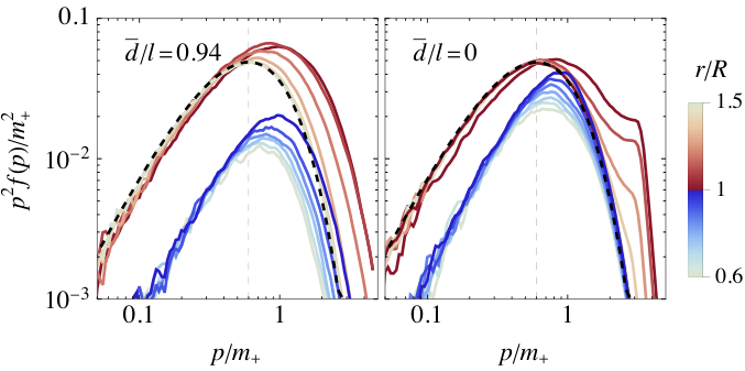
As shown in the left panel of Fig. 6, the self-interactions keep the distribution thermal around the wall. Our simulations conserve the particle number, so the momentum distribution includes a non-vanishing chemical potential around the bubble wall and inside the bubble. As high-momentum particles are more likely to penetrate the wall, the momentum distribution inside the bubble is peaked at higher momentum than outside the bubble. Allowing for strong number changing processes, the chemical potential would remain zero everywhere and the maximum of $p^{2}f(p)$ inside the bubble would move towards lower momenta, reflecting the smaller fluid energy density. In the free case, the particles making up the overdensity around the wall move away from it and rise to the high momentum bump in the right panel of Fig. 6.

We compute the particle’s mean free path $l$ in terms of their mean separation $\bar{d}\approx n_{-}^{-1/3}$ by counting the number of collisions per timestep. As shown in Fig. 7, the terminal velocity reaches a constant value if $l$ is small enough. The numerical results can be approximated well by a 4-parameter fitting function⁵⁵ 5 The fitting function can be parametrized as $a_{1}/[(1+(a_{1}-1)e^{-a_{2}\bar{d}/l})(1+a_{3}e^{-a_{4}\bar{d}/l})]$. shown with the solid curves. The velocities are shown when $R=64R_{c}$. We find that for weak self-interactions the velocity of the wall still slowly changes at the end of the simulation, indicating that the wall may always reach the same terminal velocity in infinite time. This is expected as $l$ should be compared to the thickness of the fluid shell around the wall, which increases with the bubble radius.

Fig. 7 shows that the terminal velocity can be either smaller or larger in the self-interacting case than in the free case. Interactions tend to heat the fluid and increase its number density around the wall. The first process results in a decrease in pressure, thus increasing the terminal velocity, while the latter has the opposite effect. Whether the terminal velocity increases or decreases depends on which effect dominates. The simulations indicate that stronger interactions slow down the wall if the wall moves faster than sound, i.e. , when $v_{w}\gtrsim c_{s}\approx 1/\sqrt{3}$, and speed it up otherwise.

Self-interactions make the front of the density profile steeper and decrease the energy density inside the bubble, as is shown in Fig. 8. For comparison, Fig. 8 also shows the hydrodynamic profiles for the values of $v_{w}$ and $\alpha$ corresponding to the self-interacting case. The hydrodynamic shell profile in front of the wall is considerably thinner and lighter. This is likely because we do not simulate particle number-changing processes. Such processes would heat the fluid in front of the wall, and therefore, more particles could penetrate the wall. Since a heavier shell is expected to slow down the wall more than a lighter one, the number-changing processes would also affect the terminal velocity of the wall.

The purpose of simulating particle-particle interactions is to model the effect of the collision term in the Boltzmann equation. Although currently we make several simplifying assumptions about the nature of such interactions, there are no fundamental obstacles for simulating general collision terms. In particular, the approach can be straightforwardly applied to several particle species allowing for example annihilation or bremsstrahlung processes, and interactions whose strength depends on the phase. To model quantum statistics, the collision probability can be adjusted by appropriate Bose enhancement/Pauli blocking factors estimated from the local phase space density in the simulation. Finally, the simulated particles do not have to correspond to individual particles, but to collections of particles analogously to smoothed particle hydrodynamics.