Learning Multitask Gaussian Bayesian Networks

The data analyzed in this study were obtained from the DecNef Project Brain Data Repository¹¹ 1 https://bicr-resource.atr.jp/srpbsopen/, and are a subset of the SRPBS multi-disorder MRI dataset (Tanaka et al. 2021). The rs-fMRI data for each participant at resting state were obtained using 3-Tesla Siemens whole body MRI systems at Center of Innovation in Hiroshima University. During the fMRI scan, participants were instructed to be relax, stay awake and refrain from thinking anything particular. The rs-fMRI data have the following parameters: TR = 2.5s, TE = 30ms, flip angle = $80^{\circ}$, matrix size = $64\times 64$, field of view = $212$mm, in-plane resolution = $3.3\times 3.3$, slice gap = 0.8mm, slice thickness = 3.2mm, number of slices = 40, number of volumes = 240 + 4 (dummy), total scan time = 10min + 10s (dummy). The T1-weighted images were then acquired with the following parameters: voxel size = $1\times 1\times 1$, TR = 2300ms, TE = 2.98ms, TI = 900ms; flip angle = $90^{\circ}$, FOV = $256$, matrix = $256\times 256$.

We use the rs-fMRI data of 15 MDD patients and 15 healthy control (HC) participants for the experiment. The selection criteria are as follows. The MDD patients are aged between 40 and 50, right-handed, free of other diseases, and their BDI scores are between 20 and 35. BDI is a clinical instrument for the severity of depression. The higher the score, the more severe the depression. The HC participants are selected to purposely match the MDD patients in terms of other selection criteria except for BDI score, i.e., they are in the same age cohort as the MDD patients, right-handed, free of other diseases, but with a BDI score between 0 and 7 (i.e., they do not have depression).

We applied the following pre-processing steps to the data. For each participant, 230 fMRI volumes were remained after removing the first ten volumes. Slice acquisition time and head motion were corrected on the remaining images. Participants with excessive head motion were not enrolled. The T1-weighted images use unified segment and diffeomorphic anatomical registration to guide fMRI registration through exponentiated Lie algebra as implemented in the SPM12 software²² 2 https://www.fil.ion.ucl.ac.uk/spm/software/spm12/. The rs-fMRI data were smoothed with a 6mm full-width at half-maximum Gaussian kernel and further denoised by regressing out several nuisance signals, including the Friston-24 head motion parameters and signals from cerebrospinal fluid and white matter, before linear detrending and temporal band-pass filtering ($0.01-0.08$ Hz).

After pre-processing, we select 30 brain regions (each viewed as a region of interest, ROI) based on three different network templates related to the default mode network (DMN, Raichle and Snyder 2007), including the Andrews-Hanna DMN (aDMN, Buckner, Andrews-Hanna and Schacter 2008), the dorsal DMN (dDMN, Chen et al. 2017), and the ventral DMN (vDMN, Lee, Parthasarathi and Kable 2021). Details of brain regions are presented in Table 5. The voxel-wise fMRI time courses are averaged into one regional average time course within each selected region. Then each participant’s dataset has the form of a $230\times 30$ matrix (230 sampling points in each regional average fMRI time course and 30 selected brain regions). The dataset obtained through the steps above can be reasonably considered to follow Gaussian distributions because each brain region includes at least several hundred voxels and the measurement data of each region is the regional average over the belonging voxels. Therefore, the central limit theorem is applicable. Also, such hypotheses are common for fMRI studies (Valdes-Sosa et al. 2011).

BN is a formal method to analyze decision-making strategies under uncertain conditions (Pearl 1988). Given a random vector $\boldsymbol{X}=(X_{1},\ldots,X_{p})^{\top}$, we use $\mathbb{P}(\mathbf{x})$ to denote its joint probability mass function (for the discrete case) or the joint density function (for the continuous case), where $\mathbf{x}$ is an observation of $\boldsymbol{X}$. From the chain rule of probability, we can write $\mathbb{P}(\mathbf{x})$ as

For each $X_{i}$, let $\Pi_{i}\subseteq\left\{X_{1},\ldots,X_{i-1}\right\}$ be a set of variables such that

A BN $B=(\mathcal{G},\Theta)$ can represent the joint distribution of $\boldsymbol{X}$ through a directed network model, where $\mathcal{G}$ is a network structure that encodes the assertions of conditional independence in equation (3.2), and $\Theta$ includes the parameters of the BN model corresponding to $\mathcal{G}$ (Koller and Friedman 2009). In particular, $\mathcal{G}$ is a directed acyclic graph (DAG) such that (1) each variable in $\boldsymbol{X}$ corresponds to a node in $\mathcal{G}$, and (2) the parents of the node corresponding to $X_{i}$ are the nodes corresponding to the variables in $\Pi_{i}$. Throughout this article, we use $X_{i}$ to refer to both the variable and its corresponding node in the graph. Combining equations (3.1) and (3.2), we can see that the joint distribution for $\boldsymbol{X}$ can be represented graphically by a BN, namely,

GBNs are a class of important and widely-used BNs (Geiger and Heckerman 1994). In GBNs, $\boldsymbol{X}$ follows a multivariate normal distribution $\mathcal{N}\left(\mu,\Sigma\right)$, with the joint density function

where $\mu$ is the expectation of $\boldsymbol{X}$, $\Sigma$ is the covariance matrix, and $|\Sigma|$ is the determinant of $\Sigma$. Clearly, the parameters of a GBN are $\Theta=\{\mu,\Sigma\}$.

The structure $\mathcal{G}$ and the parameters $\Theta$ can be learned from the observed data, which we call the BN learning procedure. The primary purpose of BN learning is to estimate a BN $B=(\mathcal{G},\Theta)$ that can best explain the $n$ independent observations $D=\{\mathbf{x}_{i}=(x_{i1},\dots,x_{ip})^{\top}\}_{i=1}^{n}$, leading to two major tasks: the structure learning, which attempts to learn a DAG $\mathcal{G}$ that encodes the structural dependence of the variables in $\boldsymbol{X}$, and the parameter learning, which estimates the parameters $\Theta$ associated with $\mathcal{G}$.

General machine learning methods usually require many samples to learn a robust model. In the case of insufficient data, MTL (Caruana 1997) is a general approach that incorporates task relatedness during learning and can learn robust models (Zhang and Yang 2021). Given $m$ learning tasks $\mathcal{T}=\left\{T_{1},\ldots,T_{m}\right\}$, where at least one of them is related, the aim of the MTL is to improve the performance and generalization of a model $T_{i}$ by using the knowledge contained in all or some of related $m$ tasks. The tasks in MTL can be general learning tasks such as supervised tasks (Schwab et al. 2018), unsupervised tasks (Cao et al. 2019), semi-supervised tasks (Rei 2017), reinforcement learning tasks (Teh et al. 2017), or graphical tasks (Honorio and Samaras 2010).

According to Zhang and Yang 2021, the current research of MTL focuses on characterizing the relatedness between tasks, which can be divided into three classes, including instance-based MTL (Bickel et al. 2008), feature-based MTL (Evgeniou and Pontil 2007), and parameter-based MTL (Parameswaran and Weinberger 2010). In this paper, we focus on the parameter-based MTL. The most common approach in parameter-based MTL is the task relation learning approach, which quantifies the relatedness among tasks in three ways: task similarity, task correlation, and task covariance. Early work such as Evgeniou and Pontil 2004 considers the task relations as prior information. Several studies have taken the relatedness into account by placing a common prior on model parameters of the tasks (Evgeniou et al. 2005), e.g., with Gaussian copula models (Gonçalves, Von Zuben and Banerjee 2016) and matrix generalized inverse Gaussian distribution (Li et al. 2015). However, when task relations are not available in applications, it is necessary to automatically learn task relationships from data. For instance, Williams, Bonilla and Chai 2007 proposes a multitask Gaussian process to learn task covariance from data, and Zhang and Yeung 2010 proposes a multitask generalized $t$ process by placing an inverse-Wishart prior.

The complete likelihood admits the decomposition

In Section 4 we have assumed that $\mathbb{P}\left(\Sigma_{h}\right)$ follows a uniform distribution, and to show the expressions for the remaining two parts, $\mathbb{P}\left(B_{i}\mid\Sigma_{h}\right)$ and $\mathbb{P}\left(D_{i}\mid B_{i},\Sigma_{h}\right)$, it is necessary to introduce a number of definitions and notations.

Let $\widetilde{G}$ be a decomposable undirected graph consisting of $k$ cliques in the sequence $\left\{C_{1},\ldots,C_{k}\right\}$. Define the histories of the sequence as the sets $H_{j}=\bigcup_{i=1}^{j}C_{i}$ for $j=1,\ldots,k$. Similarly, define the separators of the sequence as $S_{j}=H_{j-1}\cap C_{j}$ for $j=2,\ldots,k$. The merit of this decomposition is that we can find the corresponding low-dimensional factorization for a high-dimensional graph. For any two subsets $A$ and $B$, $S$ is said to separate $A$ and $B$, denoted by $A\perp B\mid S$, if for every node pair $a\in A$ and $b\in B$, each path connecting $a$ and $b$ includes at least one element of $S$. A probability density $\mathbb{P}$ is said to be globally Markov, if $X=(X_{A},X_{B},X_{D})\sim\mathbb{P}$ and $X_{A}\perp X_{B}\mid X_{D}$ for any triple subsets $A$, $B$, $D$ such that $A\perp B\mid D$. $X_{A}\perp X_{B}\mid X_{D}$ means that $X_{A}$ and $X_{B}$ are independent conditional on $X_{D}$. Let $\mathbb{P}_{V}$ be a joint density that is globally Markov with respect to a decomposable graph $\widetilde{G}=(V,E)$. Let $\mathcal{C}$ and $\mathcal{S}$ be the cliques and separators of $\widetilde{G}$, with corresponding marginal densities $\left\{\mathbb{P}_{C}:C\in\mathcal{C}\right\}$ and $\left\{\mathbb{P}_{S}:S\in\mathcal{S}\right\}$. Then $\mathbb{P}_{V}$ can be factorized as (Lauritzen 1996)

A BN $B$ can be transformed into a unique undirected graph $G$, also known as a moral graph. The undirected graph $G$ is generated from $B$, where if a node has more than one parent node, edges between these parent nodes are inserted, and all directed edges become undirected. As an illustration, Figure 2(a) and (b) show the transformation from a BN to an undirected graph, which is achieved by (1) adding an edge between the nodes $V_{B}$ and $V_{E}$, as both $V_{B}$ and $V_{E}$ are the parent nodes of $V_{F}$, and (2) deleting all the directions in $B$. Additionally, Figure 2(c) demonstrates that $G$ can be decomposed into four cliques and three separators.

For Gaussian graphical models, the graph structure is usually related to the inverse of the covariance matrix. Let $M$ be a $p\times p$ positive definite matrix and $A$ is an index set with $A\subset\{1,\dots,p\}$. Then we use $M_{AA}$ to denote the corresponding $|A|\times|A|$ submatrix of $M$, which is also a positive definite matrix. We are now ready to present the first main theorem based on the definitions above.

We make the following remark to further explain the implications of Theorem 5.1.

Finally, multiplying $\mathbb{P}\left(D_{i}\mid B_{i},\Sigma^{h}\right)$, $\mathbb{P}\left(B_{i}\mid\Sigma_{h}\right)$, and $\mathbb{P}\left(\Sigma_{h}\right)$, we obtain the complete likelihood function $\mathbb{P}\left(\Sigma_{h},\mathcal{D},\mathcal{B}\right)$ in (5.2).

The EM algorithm requires computing the expectation of the complete log-likelihood function with respect to the conditional distribution $\mathbb{P}\left(\Sigma_{h}\mid\mathcal{B},\mathcal{D}\right)$. As a first step, Theorem 5.3 gives its density function in a closed form.

To maximize $\mathcal{L}\left(\mathcal{B},\mathcal{D}\right)$ with respect to $\mathcal{B}$, the EM algorithm starts with an initial value $\mathcal{B}^{(0)}$, and then repeats the following two steps until convergence:

• •

  E-step: Define the function

  $$\mathcal{Q}\left(\mathcal{B}\mid\mathcal{B}^{(t-1)},\mathcal{D}\right)=\int\log\mathbb{P}\left(\Sigma_{h},\mathcal{B},\mathcal{D}\right)\mathbb{P}\left(\Sigma_{h}\mid\mathcal{B}^{(t-1)},\mathcal{D}\right)\mathrm{d}\Sigma_{h}.$$

  (5.6)

• •

  M-step: Solve the optimization problem below to generate the next iterate $\mathcal{B}^{(t)}$:

  $$\mathcal{B}^{(t)}=\underset{\mathcal{B}}{\arg\max}\ \mathcal{Q}\left(\mathcal{B}\mid\mathcal{B}^{(t-1)},\mathcal{D}\right).$$

The basic convergence properties of the EM algorithm were established by Boyles 1983 and Wu 1983, and Friedman 2013 has proved that the algorithm converges when there is no further improvement in the objective score. However, in our setting, the $\mathcal{Q}$-function in (5.6) is still intractable due to the high-dimensional integration. Instead, we view the integral in (5.6) as an expectation, and then use Monte Carlo samples to approximate it. This leads to the MCEM algorithm, which is a practical computing method for the EM algorithm.

It should be pointed out that the convergence properties of MCEM is more complicated than ordinary EM. Some efforts have been made to establish the convergence properties of MCEM; see for example Chan and Ledolter 1995 and Fort and Moulines 2003. We describe our implementation of the MCEM algorithm for MTGBN in Section 6.

The basic idea of MCEM is to replace the exact $\mathcal{Q}\left(\mathcal{B}\mid\mathcal{B}^{(t-1)},\mathcal{D}\right)$ function in (5.6) by the following unbiased estimator:

where $\{\Sigma_{h}^{l}\}_{l=1}^{N}$ is a Monte Carlo sample of $\mathbb{P}\left(\Sigma_{h}\mid\mathcal{B}^{(t-1)},\mathcal{D}\right)$. Therefore, the key to the MC E-step is a proper sampling algorithm for $\mathbb{P}\left(\Sigma_{h}\mid\mathcal{B}^{(t-1)},\mathcal{D}\right)$.

There are two main challenges that need to be addressed: (1) the positive-definiteness of $\Sigma_{h}$ must be maintained; (2) the sampling scheme needs to be fast and efficient. For the first challenge, we use the Cholesky decomposition to transform $\Sigma_{h}$ into an unrestricted vector $V$, and implement the sampling on the unrestricted space. For the second problem, we employ the HMC sampler (Neal et al. 2011) for efficient sampling, which is a powerful tool for Bayesian computation, especially in high-dimensional and other complicated scenarios. It has been empirically justified that HMC can offer greater computational efficiency than the traditional Gibbs sampling and Metropolis–Hastings algorithm.

Specifically, we factorize $\Sigma_{h}$ using the Cholesky decomposition $\Sigma_{h}=LL^{T}$, where $L$ is a lower-triangular matrix with positive diagonal elements (i.e., $l_{ii}>0$ for $i=1,2,\ldots,p$ and $l_{ij}=0$ for $i<j$). To further remove the constraints on $l_{ii}$, we work on the reparameterized variables³³ 3 The similar method is also used by the Stan software: https://mc-stan.org/docs/2_28/reference-manual/covariance-matrices-1.html., $\log(l_{ii})$, and let $V=(v_{ij})$ be a lower-triangular matrix such that $v_{ii}=\log(l_{ii})$ for $i=1,2,\ldots,p$ and $v_{ij}=l_{ij}$ for $i>j$. In this way, $V$ collects all unrestricted variables for $\Sigma_{h}$. HMC requires evaluating both $\log\mathbb{P}(V|\mathcal{B}^{(t-1)},\mathcal{D})$ and $\nabla_{V}\log\mathbb{P}(V|\mathcal{B}^{(t-1)},\mathcal{D})$, and we summarize the results in Theorem 6.1.

Based on equations (6.2) and (6.3), we can use the HMC algorithm to obtain a set of sample $V$ through iterations, denoted as $\{V^{(l)}\}_{l=1}^{N}$. Then by transfroming $V$ back to $\Sigma_{h}$, we can obtain $\{\Sigma_{h}^{(l)}\}_{l=1}^{N}$. Details of the derivation and the algorithm are given in Appendix D.

Finally in the MC M-step, we maximize the approximate $\mathcal{Q}$ function $\widetilde{\mathcal{Q}}\left(\mathcal{B}\mid\mathcal{B}^{(t-1)},\mathcal{D}\right)$ as in (6.1), and take $\mathcal{B}^{(t)}$ to be the maximizer. We use the max-min hill-climbing algorithm (MMHC, Tsamardinos, Brown and Aliferis 2006) to search the BN structures, which combines ideas from local learning, constraint-based methods, and search-and-score techniques. It has been empirically justified that on average MMHC outperforms several prototypical algorithms (Wang 2018), such as PC (Kalisch and Bühlman 2007), sparse candidate (Friedman, Nachman and Pe’er 2013), greedy equivalence search (Ramsey et al. 2017), and greedy search (Chickering 2002).

It is observed that $\{B^{(t-1)}_{i}\}_{i=1}^{m}$ are independent with each other in the objective function $\widetilde{\mathcal{Q}}\left(\mathcal{B}\mid\mathcal{B}^{(t-1)},\mathcal{D}\right)$. Therefore, we can apply MMHC $m$ times on the $m$ independent sub-problems:

The overall MCEM algorithm of MTGBN is thereby given in Algorithm 1.

We simulate synthetic datasets with our data generation mechanism (see Figure 1). First, we random generate $\Sigma_{h}$ from the uniform distribution over all $p\times p$ positive definite matrices with unit trace, using an approach similar to Mittelbach, Matthiesen and Jorswieck 2012. Then given $\Sigma_{h}$, we sample $m$ intermediate matrices $\{\tilde{\Sigma}_{l}\}_{l=1}^{m}$ from $IW\left(\Sigma_{h},\nu_{0}\right)$, so each $\tilde{\Sigma}_{l}$ is a $p\times p$ positive definite matrix.

The $m$ undirected graph structures $\left\{G_{l}\right\}_{l=1}^{m}$ are defined as follows. For each $l=1,\dots,m$, let $\tilde{\Omega}_{l}=(\tilde{\omega}_{ij,l})=\tilde{\Sigma}_{l}^{-1}\in\mathbb{R}^{p\times p}$, $V=\{1,\ldots,p\}$, and define $E_{l}=\{(i,j):i\neq j,|\tilde{\omega}_{ij,l}|>t_{l}\}$, where $t_{l}>0$ is a threshold to control the density of $E_{l}$. Let $\Omega_{l}=(\omega_{ij,l})$ be a matrix such that $\omega_{ii,l}=\tilde{\omega}_{ii,l}$, $\omega_{ij,l}=\tilde{\omega}_{ij,l}$ if $(i,j)\in E_{l}$, and $\omega_{ij,l}=0$ otherwise. We assume that $\Omega_{l}$ is still positive definite, which can be achieved by repeatedly sampling $\tilde{\Sigma}_{l}$ until the condition is met. Then the graphs are given by $G_{l}=(V,E_{l})$.

Denote by $|E_{l}|$ the cardinality of $E_{l}$, so $d_{l}=|E_{l}|/p^{2}$ represents the density of $G_{l}$, and is dependent on the threshold $t_{l}$. By adjusting $t_{l}$, we can obtain $G_{l}$ with different density levels. In fact, the zero elements in $\Omega_{l}$ imply the conditional independence structure of the variables in $G_{l}$ (Dawid and Lauritzen 1993).

Finally, we generate $m$ independent datasets $\left\{D_{l}\right\}_{l=1}^{m}$ by sampling each $D_{l}=\left\{\mathbf{x}_{l1},\ldots,\mathbf{x}_{ln_{l}}\right\}$ from a multivariate normal distribution $\mathcal{N}\left(0,\Sigma_{l}\right)$, where $\Sigma_{l}=\Omega_{l}^{-1}$, and $n_{l}$ is the sample size for the $l$-th dataset.

To evaluate and compare the performance of the MTGBN method, we also learn each network independently with single-task learning (SIG for short), and learn a common network structure for all contexts (AVG for short), i.e., an “average” network that treats all subjects as samples in one task. AVG was previously used as a baseline in Oyen and Lane 2012. To compare the performance of MTGBN, SIG, and AVG, especially on the differences between the structures, we use edge error, edge precision, edge F-score, and edge distance as the primary evaluation measures.

Let $\left\{B_{output,l}\right\}_{l=1}^{m}$ represent the $m$ BN structures obtained from MTGBN, SIG, or AVG method, and $\left\{G_{output,l}\right\}_{l=1}^{m}$ be the undirected graph structures corresponding to $\left\{B_{output,l}\right\}_{l=1}^{m}$. In the experiment of synthetic data, since the generated networks $\left\{G_{l}\right\}_{l=1}^{m}$ are undirected graphs, we mainly evaluate the network structures without considering the edge orientation, which we call the adjacency measure. To compute the evaluation metrics, we first calculate four basic statistics: true positives (TP), the number of edges that are both in $G_{output,1}$ and $G_{1}$; false positives (FP), the number of edges that are present in $G_{output,1}$ but not in $G_{1}$; false negatives (FN), the number of edges that are present in $G_{1}$ but not in $G_{output,1}$; and true negatives (TN), the number of vertex pairs that are neither edges in $G_{1}$ nor in $G_{output,1}$. Then the edge adjacency error, edge adjacency precision, edge adjacency F-score, and edge adjacency distance are defined as:

• •

  Error:

  $$\text{\emph{Error}}=\frac{FP+FN}{TP+TN+FP+FN}.$$

  (7.1)

• •

  Precision:

  $$\text{ \emph{Precision} }=\frac{TP}{TP+FP}.$$

• •

  F-score:

  $$\text{ \emph{F-score}}=2\cdot\frac{\text{ \emph{Precision} }\cdot\text{\emph{Recall} }}{\text{ \emph{Precision} }+\text{\emph{Recall}}},$$

  where $\text{ \emph{Recall}}=TP/(TP+FN)$.

• •

  Edge distance: Given two structures, this measure is the minimum number of edges needed to convert the learned graph into the true one.

We compare the performance of MTGBN, SIG, and AVG on the following three aspects.

Performance v.s. sample size: We fix the task number $m=10$, number of nodes $p=15$, density level $d_{l}=0.3$, and compare the model performance of network structure learning for different sample size $n_{l}=50,100,150,200,250,300$.

Performance v.s. task number: We fix the number of nodes $p=15$, density level $d_{l}=0.3$, sample size $n_{l}=250$, and consider different task number $m=2,4,6,8,10$.

Performance v.s. density level: We fix the task number $m=10$, number of nodes $p=15$, and consider a combination of different sample size $n_{l}=100,200,300$ and density levels ranging from $0.2$ to $0.6$.

The evaluation metrics for one simulation run are averaged over the $m$ datasets, and we repeat each experiment $10$ times. The final evaluation metrics are thereby averaged over the $10$ simulation runs.

In this experiment, we select benchmark networks from the Bayesian Network Repository (Constantinou et al. 2020). We choose three medium-sized benchmark networks and generate low sample size data to validate our assumption that the proposed MTGBN method can improve the understanding of the underlying structure and generalize better even at small sample sizes. The information of the selected benchmark networks is provided in Table 1.

To obtain a set of related networks, we apply perturbations to the given benchmark network to create similar but different networks. Denote by $B_{truth}$ the benchmark BN with an adjacency matrix $A_{t}=(a^{t}_{ij})\in\mathbb{R}^{p\times p}$, where $a^{t}_{ij}=1$ if there is an edge from node $i$ to node $j$, and $a^{t}_{ij}=0$ otherwise, $i,j=1,\ldots,p$. Then the generated BN, denoted by $B_{gen}$, is constructed in the following way. Let $A_{g}$ be the adjacency matrix of $B_{gen}$, and define the perturbation level as the ratio of the number of changed edges in $A_{g}$ to the number of all possible edges. For example, if the perturbation level is $30\%$, we first set $A_{g}=A_{t}$, and then randomly select $30\%$ of the off-diagonal elements $a^{t}_{ij}(i\neq j)$ in $A_{t}$. For each selected element $a^{t}_{ij}$, if $a^{t}_{ij}=0$, then we set $a^{g}_{ij}=1$ (adding edge); if $a^{t}_{ij}=1$, then with probability $1/2$ we set $a^{g}_{ij}=0$ (deleting edge), otherwise let $a^{g}_{ji}=1$ (reversing edge). For each benchmark BN, we generate $m$ networks by such a perturbation scheme, and in our experiment we set $m=10$. Each set of generated networks can be viewed as a class of tasks sharing the same prior, since they are generated from the same benchmark BN. Then we simulate data for each generated BN with a sample size $n_{l}=250,l=1,\dots,m$.

We mainly compare the edge arrowhead error under different network perturbation levels in the benchmark network experiment. The edge arrowhead error is the same as equation (7.1), except that TP, FP, FN, and TN are calculated considering the edge orientation. Same as Section 7.1, we repeat the experiment 10 times and compute the averaged errors for MTGBN, SIG, and AVG.

In the synthetic data experiment, we first evaluate the performance of the proposed MTGBN method under different sample sizes, with the results shown in Figure 3. It is clear that MTGBN significantly outperforms the other two methods. The average edge adjacency error of MTGBN under different sample sizes is in the range of 0.03 - 0.06, whereas for SIG, even using five times the number of training data (sample size $=250$), its average edge adjacency error is still larger than MTGBN (sample size $=50$). The same trend is observed in the edge adjacency distance. For the other two metrics, MTGBN consistently results in higher average edge adjacency precision and F-score than AVG and SIG. Compared with SIG, the average edge adjacency precision of MTGBN is also more stable under different sample sizes, and the best result is achieved at the sample size of 200. Such findings show that the proposed MTGBN method can produce satisfactory results using a small amount of data, thereby demonstrating its usefulness in cases where data are expensive or hard to collect.

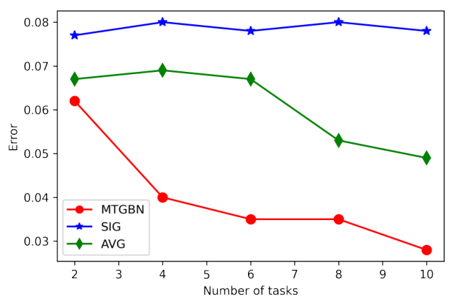
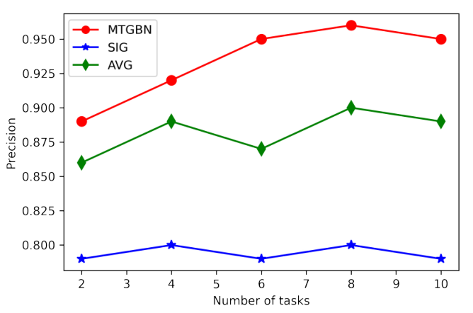
We also compare the performance of MTGBN, AVG, and SIG under different task numbers $m$. Figure 4 indicates that MTGBN performs better than AVG and SIG for all the test cases. As expected, SIG does not have better performance at a larger value of $m$, since it only utilizes the information of a single task. In contrast, MTGBN can use the information of related tasks, thus leading to increased performance. We find that MTGBN can already get a good result when $m=4$, and with the increase of $m$, the performance tends to be stable. These results are also consistent with the existing literature (Oyen and Lane 2012).

In addition to the sample size and task number, we find that the network density also affects the model’s performance. We compare the average edge adjacency error of MTGBN, AVG, and SIG under different sample sizes and density levels, with results shown in Figure 5. It can be seen that with the increase in sample size and decrease in density, the edge adjacency error of the model gets smaller. Such a phenomenon is more obvious in MTGBN. Compared with AVG and SIG, the proposed MTGBN method is especially advantageous with a small sample size ($n_{l}=100$) and a medium density ($d_{l}=0.4$).

In the experiment of the benchmark network data, we compare the average arrowhead errors for MTGBN, AVG, and SIG, and show the results in Table 2. We consider four perturbation levels, $5\%$, $10\%$, $20\%$, and $30\%$, representing the proportion of possible edges that are randomly modified during simulation. Again, the comparison demonstrates that MTGBN is better than SIG and AVG all the time. Even at a high perturbation level of $30\%$, MTGBN still has decent error rates, whereas SIG and AVG do not provide good results. We also find that the more related the tasks are, the better results MTGBN can achieve.

References

- Altendorf, Restificar and Dietterich (2005) Altendorf, E. E., Restificar, A. C. and Dietterich, T. G. (2005). Learning from sparse data by exploiting monotonicity constraints. In Proceedings of the Twenty-First Conference on Uncertainty in Artificial Intelligence 18–26.
- Andrews-Hanna, Smallwood and Spreng (2014) [author] Andrews-Hanna, Jessica RJ. R., Smallwood, JonathanJ. and Spreng, R NathanR. N. (2014). The default network and self-generated thought: component processes, dynamic control, and clinical relevance. Annals of the New York Academy of Sciences 1316 29–52.
- Andrews-Hanna et al. (2010) [author] Andrews-Hanna, Jessica RJ. R., Reidler, Jay SJ. S., Sepulcre, JorgeJ., Poulin, ReneeR. and Buckner, Randy LR. L. (2010). Functional-anatomic fractionation of the brain’s default network. Neuron 65 550–562.
- Aragam, Gu and Zhou (2017) [author] Aragam, BryonB., Gu, JiayingJ. and Zhou, QingQ. (2017). Learning large-scale Bayesian networks with the sparsebn package. arXiv preprint arXiv:1703.04025.
- Beijers et al. (2019) [author] Beijers, LianL., Wardenaar, Klaas JK. J., van Loo, Hanna MH. M. and Schoevers, Robert AR. A. (2019). Data-driven biological subtypes of depression: systematic review of biological approaches to depression subtyping. Molecular Psychiatry 24 888–900.
- Belleau, Taubitz and Larson (2015) [author] Belleau, Emily LE. L., Taubitz, Lauren EL. E. and Larson, Christine LC. L. (2015). Imbalance of default mode and regulatory networks during externally focused processing in depression. Social Cognitive and Affective Neuroscience 10 744–751.
- Bickel et al. (2008) Bickel, S., Bogojeska, J., Lengauer, T. and Scheffer, T. (2008). Multi-task learning for HIV therapy screening. In Proceedings of the 25th International Conference on Machine Learning 56–63.
- Bielza and Larranaga (2014) [author] Bielza, ConchaC. and Larranaga, PedroP. (2014). Bayesian networks in neuroscience: a survey. Frontiers in Computational Neuroscience 8 131–153.
- Bluhm et al. (2009) [author] Bluhm, RobynR., Williamson, PeterP., Lanius, RuthR., Théberge, JeanJ., Densmore, MariaM., Bartha, RobertR., Neufeld, RichardR. and Osuch, ElizabethE. (2009). Resting state default-mode network connectivity in early depression using a seed region-of-interest analysis: Decreased connectivity with caudate nucleus. Psychiatry and Clinical Neurosciences 63 754–761.
- Boyles (1983) [author] Boyles, Russell AR. A. (1983). On the convergence of the EM algorithm. Journal of the Royal Statistical Society: Series B (Methodological) 45 47–50.
- Buckner, Andrews-Hanna and Schacter (2008) [author] Buckner, Randy LR. L., Andrews-Hanna, Jessica RJ. R. and Schacter, Daniel LD. L. (2008). The brain’s default network: anatomy, function, and relevance to disease. Annals of the New York Academy of Sciences 1124 1–38.
- Cao et al. (2019) [author] Cao, WenmingW., Qian, ShengS., Wu, SiS. and Wong, Hau-SanH.-S. (2019). Unsupervised multi-task learning with hierarchical data structure. Pattern Recognition 86 248–264.
- Caruana (1997) [author] Caruana, RichR. (1997). Multitask learning. Machine learning 28 41–75.
- Chan and Ledolter (1995) [author] Chan, KSK. and Ledolter, JohannesJ. (1995). Monte Carlo EM estimation for time series models involving counts. Journal of the American Statistical Association 90 242–252.
- Chen et al. (2017) [author] Chen, Jingyuan EJ. E., Glover, Gary HG. H., Greicius, Michael DM. D. and Chang, CatieC. (2017). Dissociated patterns of anti-correlations with dorsal and ventral default-mode networks at rest. Human Brain Mapping 38 2454–2465.
- Chen et al. (2021) [author] Chen, HaoH., Guo, YingY., He, YongY., Liu, DongD., Liu, LeiL. and Zhou, Xiao-HuaX.-H. (2021). Joint Learning of Multiple Differential Networks with fMRI data for Brain Connectivity Alteration Detection. arXiv preprint arXiv:2106.03334.
- Chickering (2002) [author] Chickering, David MaxwellD. M. (2002). Optimal structure identification with greedy search. Journal of Machine Learning Research 3 507–554.
- Constantinou et al. (2020) [author] Constantinou, ACA., Liu, YY., Chobtham, KK., Guo, ZZ. and Kitson, NKN. (2020). The Bayesys data and Bayesian network repository. Queen Mary University of London: London, UK.
- Cooper and Herskovits (1992) [author] Cooper, Gregory FG. F. and Herskovits, EdwardE. (1992). A Bayesian method for the induction of probabilistic networks from data. Machine Learning 9 309–347.
- Dawid and Lauritzen (1993) [author] Dawid, A PhilipA. P. and Lauritzen, Steffen LS. L. (1993). Hyper Markov laws in the statistical analysis of decomposable graphical models. The Annals of Statistics 21 1272–1317.
- Dempster, Laird and Rubin (1977) [author] Dempster, Arthur PA. P., Laird, Nan MN. M. and Rubin, Donald BD. B. (1977). Maximum likelihood from incomplete data via the EM algorithm. Journal of the Royal Statistical Society: Series B (Methodological) 39 1–22.
- Etkin, Egner and Kalisch (2011) [author] Etkin, AmitA., Egner, TobiasT. and Kalisch, RaffaelR. (2011). Emotional processing in anterior cingulate and medial prefrontal cortex. Trends in Cognitive Sciences 15 85–93.
- Evgeniou and Pontil (2004) Evgeniou, T. and Pontil, M. (2004). Regularized multi–task learning. In Proceedings of the Tenth ACM SIGKDD International Conference on Knowledge Discovery and Data mining 109–117.
- Evgeniou and Pontil (2007) [author] Evgeniou, AnA. and Pontil, MassimilianoM. (2007). Multi-task feature learning. Advances in Neural Information Processing Systems 19.
- Evgeniou et al. (2005) [author] Evgeniou, TheodorosT., Micchelli, Charles AC. A., Pontil, MassimilianoM. and Shawe-Taylor, JohnJ. (2005). Learning multiple tasks with kernel methods. Journal of Machine Learning Research 6 615–637.
- Fort and Moulines (2003) [author] Fort, GersendeG. and Moulines, EricE. (2003). Convergence of the Monte Carlo expectation maximization for curved exponential families. The Annals of Statistics 31 1220–1259.
- Friedman (2013) [author] Friedman, NirN. (2013). The Bayesian structural EM algorithm. arXiv preprint arXiv:1301.7373.
- Friedman, Nachman and Pe’er (2013) [author] Friedman, NirN., Nachman, IftachI. and Pe’er, DanaD. (2013). Learning Bayesian network structure from massive datasets: The" sparse candidate" algorithm. arXiv preprint arXiv:1301.6696.
- Fu et al. (2008) [author] Fu, Cynthia HYC. H., Mourao-Miranda, JanainaJ., Costafreda, Sergi GS. G., Khanna, AkashA., Marquand, Andre FA. F., Williams, Steve CRS. C. and Brammer, Michael JM. J. (2008). Pattern classification of sad facial processing: toward the development of neurobiological markers in depression. Biological Psychiatry 63 656–662.
- Gámez, Mateo and Puerta (2011) [author] Gámez, José AJ. A., Mateo, Juan LJ. L. and Puerta, José MJ. M. (2011). Learning Bayesian networks by hill climbing: efficient methods based on progressive restriction of the neighborhood. Data Mining and Knowledge Discovery 22 106–148.
- Geiger and Heckerman (1994) [author] Geiger, DanD. and Heckerman, DavidD. (1994). Learning gaussian networks. In Uncertainty Proceedings 1994 235–243. Elsevier.
- Geiger et al. (1997) [author] Geiger, DanD., Heckerman, DavidD. et al. (1997). A characterization of the Dirichlet distribution through global and local parameter independence. Annals of Statistics 25 1344–1369.
- Gonçalves, Von Zuben and Banerjee (2016) [author] Gonçalves, André RA. R., Von Zuben, Fernando JF. J. and Banerjee, ArindamA. (2016). Multi-task sparse structure learning with gaussian copula models. The Journal of Machine Learning Research 17 1205–1234.
- Greicius et al. (2007) [author] Greicius, Michael DM. D., Flores, Benjamin HB. H., Menon, VinodV., Glover, Gary HG. H., Solvason, Hugh BH. B., Kenna, HeatherH., Reiss, Allan LA. L. and Schatzberg, Alan FA. F. (2007). Resting-state functional connectivity in major depression: abnormally increased contributions from subgenual cingulate cortex and thalamus. Biological Psychiatry 62 429–437.
- He et al. (2021) [author] He, YongY., Li, QiushiQ., Hu, QinqinQ. and Liu, LeiL. (2021). Transfer Learning in High-dimensional Semi-parametric Graphical Models with Application to Brain Connectivity Analysis. arXiv preprint arXiv:2112.13356.
- Heckerman, Geiger and Chickering (1995) [author] Heckerman, DavidD., Geiger, DanD. and Chickering, David MD. M. (1995). Learning Bayesian networks: The combination of knowledge and statistical data. Machine Learning 20 197–243.
- Honorio and Samaras (2010) Honorio, J. and Samaras, D. (2010). Multi-task learning of Gaussian graphical models. In ICML.
- Ji, Xia and Meng (2015) Ji, Z., Xia, Q. and Meng, G. (2015). A review of parameter learning methods in Bayesian network. In International Conference on Intelligent Computing 3–12. Springer.
- Kalisch and Bühlman (2007) [author] Kalisch, MarkusM. and Bühlman, PeterP. (2007). Estimating high-dimensional directed acyclic graphs with the PC-algorithm. Journal of Machine Learning Research 8 613–636.
- Khundakar and Thomas (2009) [author] Khundakar, Ahmad AA. A. and Thomas, Alan JA. J. (2009). Morphometric changes in early-and late-life major depressive disorder: evidence from postmortem studies. International Psychogeriatrics 21 844–854.
- Koller and Friedman (2009) [author] Koller, DaphneD. and Friedman, NirN. (2009). Probabilistic graphical models: principles and techniques. MIT press.
- Koski and Noble (2012) [author] Koski, Timo JTT. J. and Noble, JohnJ. (2012). A review of Bayesian networks and structure learning. Mathematica Applicanda 40 51–103.
- Lauritzen (1996) [author] Lauritzen, Steffen LS. L. (1996). Graphical models 17. Clarendon Press.
- Lee, Parthasarathi and Kable (2021) [author] Lee, SangilS., Parthasarathi, TrishalaT. and Kable, Joseph WJ. W. (2021). The ventral and dorsal default mode networks are dissociably modulated by the vividness and valence of imagined events. Journal of Neuroscience 41 5243–5250.
- Lemogne et al. (2009) [author] Lemogne, CédricC., le Bastard, GuillaumeG., Mayberg, HelenH., Volle, EmmanuelleE., Bergouignan, LoretxuL., Lehéricy, StéphaneS., Allilaire, Jean-FrançoisJ.-F. and Fossati, PhilippeP. (2009). In search of the depressive self: extended medial prefrontal network during self-referential processing in major depression. Social Cognitive and Affective Neuroscience 4 305–312.
- Li et al. (2015) [author] Li, YingmingY., Yang, MingM., Qi, ZhongangZ. and Zhang, Zhongfei MarkZ. M. (2015). Bayesian multi-task relationship learning with link structure. IEEE Transactions on Knowledge and Data Engineering 28 873–887.
- Li et al. (2018) [author] Li, Bao-JuanB.-J., Friston, KarlK., Mody, MariaM., Wang, Hua-NingH.-N., Lu, Hong-BingH.-B. and Hu, De-WenD.-W. (2018). A brain network model for depression: From symptom understanding to disease intervention. CNS Neuroscience & Therapeutics 24 1004–1019.
- Liu et al. (2013) [author] Liu, FengF., Guo, WenbinW., Liu, LingL., Long, ZhiliangZ., Ma, ChaoqiongC., Xue, ZhiminZ., Wang, YifengY., Li, JunJ., Hu, MaorongM., Zhang, JianweiJ. et al. (2013). Abnormal amplitude low-frequency oscillations in medication-naive, first-episode patients with major depressive disorder: a resting-state fMRI study. Journal of Affective Disorders 146 401–406.
- Marreiros, Kiebel and Friston (2008) [author] Marreiros, André CA. C., Kiebel, Stefan JS. J. and Friston, Karl JK. J. (2008). Dynamic causal modelling for fMRI: a two-state model. Neuroimage 39 269–278.
- Mittelbach, Matthiesen and Jorswieck (2012) [author] Mittelbach, MartinM., Matthiesen, BhoB. and Jorswieck, Eduard AE. A. (2012). Sampling uniformly from the set of positive definite matrices with trace constraint. IEEE Transactions on Signal Processing 60 2167–2179.
- Moreira et al. (2016) Moreira, M. W., Rodrigues, J. J., Oliveira, A. M., Ramos, R. F. and Saleem, K. (2016). A preeclampsia diagnosis approach using Bayesian networks. In 2016 IEEE International Conference on Communications (ICC) 1–5. IEEE.
- Muirhead (2009) [author] Muirhead, Robb JR. J. (2009). Aspects of multivariate statistical theory. John Wiley & Sons.
- Neal et al. (2011) [author] Neal, Radford MR. M. et al. (2011). MCMC using Hamiltonian dynamics. Handbook of Markov Chain Monte Carlo 11.
- Oyen and Lane (2012) Oyen, D. and Lane, T. (2012). Leveraging domain knowledge in multitask Bayesian network structure learning. In Proceedings of the AAAI Conference on Artificial Intelligence 26.
- Parameswaran and Weinberger (2010) [author] Parameswaran, ShibinS. and Weinberger, Kilian QK. Q. (2010). Large margin multi-task metric learning. Advances in Neural Information Processing Systems 23 1867–1875.
- Pearl (1988) [author] Pearl, JudeaJ. (1988). Probabilistic reasoning in intelligent systems: networks of plausible inference. Morgan kaufmann.
- Raichle and Snyder (2007) [author] Raichle, Marcus EM. E. and Snyder, Abraham ZA. Z. (2007). A default mode of brain function: a brief history of an evolving idea. Neuroimage 37 1083–1090.
- Ramsey et al. (2017) [author] Ramsey, JosephJ., Glymour, MadelynM., Sanchez-Romero, RubenR. and Glymour, ClarkC. (2017). A million variables and more: the fast greedy equivalence search algorithm for learning high-dimensional graphical causal models, with an application to functional magnetic resonance images. International Journal of Data Science and Analytics 3 121–129.
- Rei (2017) Rei, M. (2017). Semi-supervised Multitask Learning for Sequence Labeling. In Proceedings of the 55th Annual Meeting of the Association for Computational Linguistics (Volume 1: Long Papers) 2121–2130.
- Robert (2014) [author] Robert, ChristianC. (2014). Machine learning, a probabilistic perspective.
- Schwab et al. (2018) Schwab, P., Keller, E., Muroi, C., Mack, D. J., Strässle, C. and Karlen, W. (2018). Not to cry wolf: Distantly supervised multitask learning in critical care. In International Conference on Machine Learning 4518–4527. PMLR.
- Schwarz et al. (1978) [author] Schwarz, GideonG. et al. (1978). Estimating the dimension of a model. Annals of Statistics 6 461–464.
- Seth (2010) [author] Seth, Anil KA. K. (2010). A MATLAB toolbox for Granger causal connectivity analysis. Journal of Neuroscience Methods 186 262–273.
- Sheline et al. (2010) [author] Sheline, Yvette IY. I., Price, Joseph LJ. L., Yan, ZhiziZ. and Mintun, Mark AM. A. (2010). Resting-state functional MRI in depression unmasks increased connectivity between networks via the dorsal nexus. Proceedings of the National Academy of Sciences 107 11020–11025.
- Smith et al. (2013) [author] Smith, Stephen MS. M., Vidaurre, DiegoD., Beckmann, Christian FC. F., Glasser, Matthew FM. F., Jenkinson, MarkM., Miller, Karla LK. L., Nichols, Thomas ET. E., Robinson, Emma CE. C., Salimi-Khorshidi, GholamrezaG., Woolrich, Mark WM. W. et al. (2013). Functional connectomics from resting-state fMRI. Trends in Cognitive Sciences 17 666–682.
- Spirtes and Glymour (1991) [author] Spirtes, PeterP. and Glymour, ClarkC. (1991). An algorithm for fast recovery of sparse causal graphs. Social Science Computer Review 9 62–72.
- Spirtes et al. (2000) [author] Spirtes, PeterP., Glymour, Clark NC. N., Scheines, RichardR. and Heckerman, DavidD. (2000). Causation, Prediction, and Search. MIT press.
- Tanaka et al. (2021) [author] Tanaka, Saori CS. C., Yamashita, AyumuA., Yahata, NoriakiN., Itahashi, TakashiT., Lisi, GiuseppeG., Yamada, TakashiT., Ichikawa, NahoN., Takamura, MasahiroM., Yoshihara, YujiroY., Kunimatsu, AkiraA. et al. (2021). A multi-site, multi-disorder resting-state magnetic resonance image database. Scientific data 8 1–15.
- Teh et al. (2017) [author] Teh, Yee WhyeY. W., Bapst, VictorV., Czarnecki, Wojciech MarianW. M., Quan, JohnJ., Kirkpatrick, JamesJ., Hadsell, RaiaR., Heess, NicolasN. and Pascanu, RazvanR. (2017). Distral: Robust multitask reinforcement learning. arXiv preprint arXiv:1707.04175.
- Tsamardinos, Brown and Aliferis (2006) [author] Tsamardinos, IoannisI., Brown, Laura EL. E. and Aliferis, Constantin FC. F. (2006). The max-min hill-climbing Bayesian network structure learning algorithm. Machine Learning 65 31–78.
- Valdes-Sosa et al. (2011) [author] Valdes-Sosa, Pedro AP. A., Roebroeck, AlardA., Daunizeau, JeanJ. and Friston, KarlK. (2011). Effective connectivity: influence, causality and biophysical modeling. Neuroimage 58 339–361.
- Wang (2018) Wang, Y. (2018). Analysis of the Max-Min Hill-Climbing Algorithm. In 2018 International Conference on Transportation & Logistics, Information & Communication, Smart City (TLICSC 2018) 509–511. Atlantis Press.
- Wei and Tanner (1990) [author] Wei, Greg CGG. C. and Tanner, Martin AM. A. (1990). A Monte Carlo implementation of the EM algorithm and the poor man’s data augmentation algorithms. Journal of the American statistical Association 85 699–704.
- Williams, Bonilla and Chai (2007) [author] Williams, ChrisC., Bonilla, Edwin VE. V. and Chai, Kian MK. M. (2007). Multi-task Gaussian process prediction. Advances in Neural Information Processing Systems 153–160.
- Wu (1983) [author] Wu, CF JeffC. J. (1983). On the convergence properties of the EM algorithm. The Annals of Statistics 95–103.
- Wu et al. (2011) [author] Wu, Qi-ZhuQ.-Z., Li, Dong-MingD.-M., Kuang, Wei-HongW.-H., Zhang, Ti-JiangT.-J., Lui, SuS., Huang, Xiao-QiX.-Q., Chan, Raymond CKR. C., Kemp, Graham JG. J. and Gong, Qi-YongQ.-Y. (2011). Abnormal regional spontaneous neural activity in treatment-refractory depression revealed by resting-state fMRI. Human Brain Mapping 32 1290–1299.
- Xia and He (2017) [author] Xia, MingruiM. and He, YongY. (2017). Functional connectomics from a “big data” perspective. Neuroimage 160 152–167.
- Yamashita et al. (2020) [author] Yamashita, AyumuA., Sakai, YukiY., Yamada, TakashiT., Yahata, NoriakiN., Kunimatsu, AkiraA., Okada, NaohiroN., Itahashi, TakashiT., Hashimoto, RyuichiroR., Mizuta, HirotoH., Ichikawa, NahoN. et al. (2020). Generalizable brain network markers of major depressive disorder across multiple imaging sites. PLoS biology 18 e3000966.
- Yamashita et al. (2021) [author] Yamashita, AyumuA., Sakai, YukiY., Yamada, TakashiT., Yahata, NoriakiN., Kunimatsu, AkiraA., Okada, NaohiroN., Itahashi, TakashiT., Hashimoto, RyuichiroR., Mizuta, HirotoH., Ichikawa, NahoN. et al. (2021). Common Brain Networks Between Major Depressive-Disorder Diagnosis and Symptoms of Depression That Are Validated for Independent Cohorts. Frontiers in Psychiatry 12 1–14.
- Yan et al. (2019) [author] Yan, Chao-GanC.-G., Chen, XiaoX., Li, LeL., Castellanos, Francisco XavierF. X., Bai, Tong-JianT.-J., Bo, Qi-JingQ.-J., Cao, JunJ., Chen, Guan-MaoG.-M., Chen, Ning-XuanN.-X., Chen, WeiW. et al. (2019). Reduced default mode network functional connectivity in patients with recurrent major depressive disorder. Proceedings of the National Academy of Sciences 116 9078–9083.
- Young et al. (2016) [author] Young, CBC., Chen, TT., Nusslock, RR., Keller, JJ., Schatzberg, AFA. and Menon, VV. (2016). Anhedonia and general distress show dissociable ventromedial prefrontal cortex connectivity in major depressive disorder. Translational Psychiatry 6 e810.
- Zamoscik et al. (2014) [author] Zamoscik, VeraV., Huffziger, SilkeS., Ebner-Priemer, UlrichU., Kuehner, ChristineC. and Kirsch, PeterP. (2014). Increased involvement of the parahippocampal gyri in a sad mood predicts future depressive symptoms. Social Cognitive and Affective Neuroscience 9 2034–2040.
- Zarikas, Papageorgiou and Regner (2015) [author] Zarikas, VasiliosV., Papageorgiou, ElpinikiE. and Regner, PeterP. (2015). Bayesian network construction using a fuzzy rule based approach for medical decision support. Expert Systems 32 344–369.
- Zhang and Yang (2021) [author] Zhang, YuY. and Yang, QiangQ. (2021). A survey on multi-task learning. IEEE Transactions on Knowledge and Data Engineering.
- Zhang and Yeung (2010) Zhang, Y. and Yeung, D.-Y. (2010). Multi-task learning using generalized t process. In Proceedings of the Thirteenth International Conference on Artificial Intelligence and Statistics 964–971. JMLR Workshop and Conference Proceedings.
- Zhao et al. (2014) [author] Zhao, Y-JY.-J., Du, M-YM.-Y., Huang, X-QX.-Q., Lui, SS., Chen, Z-QZ.-Q., Liu, JJ., Luo, YY., Wang, X-LX.-L., Kemp, GJG. and Gong, Q-YQ.-Y. (2014). Brain grey matter abnormalities in medication-free patients with major depressive disorder: a meta-analysis. Psychological Medicine 44 2927–2937.