跳到论文正文
W Papers独立论文阅读器 arXiv:2205.05341 论文正文 计算阅读时间 · 0%
引用这篇论文根据当前论文元数据生成,正式投稿前建议核对。


License: CC BY-NC-ND 4.0
arXiv:2205.05341v1 [math.ST] 11 May 2022

A zero-estimator approach for estimating the signal level in a high-dimensional model-free setting

Ilan Livne, David Azriel, Yair Goldberg Affiliation: Technion - Israel Institute of Technology
August 11, 2026
Abstract

We study a high-dimensional regression setting under the assumption of known covariate distribution. We aim at estimating the amount of explained variation in the response by the best linear function of the covariates (the signal level). In our setting, neither sparsity of the coefficient vector, nor normality of the covariates or linearity of the conditional expectation are assumed. We present an unbiased and consistent estimator and then improve it by using a zero-estimator approach, where a zero-estimator is a statistic whose expected value is zero. More generally, we present an algorithm based on the zero estimator approach that in principle can improve any given estimator. We study some asymptotic properties of the proposed estimators and demonstrate their finite sample performance in a simulation study.

Key words and phrases: Linear Projection, Semi-supervised setting, U-statistics, Variance estimation, Zero-estimators.

1 Introduction

In many regression settings, an important goal is to estimate the signal and noise levels, i.e., to quantify the amount of variance in the response variable that can be explained by a set of covariates, versus how much of the variation is left unexplained. When the covariates’ dimension is low and a linear regression model is assumed, the ordinary least squares method can be used to find a consistent estimator for the signal level. However, in a high-dimensional setting, the least squares method breaks down and it becomes more challenging to develop good estimators without further assumptions. In recent years, several methods have been proposed for estimating the signal level under the assumption that the regression coefficient vector β\beta is sparse (Fan et al. 2012; Sun and Zhang 2012; Chatterjee and Jafarov 2015; Verzelen et al. 2018; Cai and Guo 2020). Other widely-used methods assume some probabilistic structure on β\beta (e.g., β\beta is Gaussian) and use maximum likelihood to derive consistent estimators of the signal level (Yang et al. 2010; Bonnet et al. 2015). These methods have been extensively studied in the literature of random-effect models where β\beta is treated as random; see de Los Campos et al. 2015 and references therein. However, methods that rely on the assumption that β\beta is either sparse or highly structured may not perform well when these assumptions fail to hold. For example, a known problem in genetics is the problem of missing heritability (de Los Campos et al. 2015; Zhu and Zhou 2020). Heritability is defined as the fraction of the observed outcome (phenotype) that is explained by genetic factors. The term “missing heritability” is traditionally used to describe the gap between heritability estimates from genome-wide-association-studies (GWAS) and the corresponding estimates from family studies. To explain the gap, it has been suggested that some phenotypes are explained by a numerous number of genetic factors that their individual effect is too small to detect, but their collective effect is significant (Yang et al. 2010; Young 2022). In such a setting, methods that rely on the sparsity assumption may fail to provide accurate estimates.

Rather than assuming sparsity or other structural assumptions on β\beta, a different approach for estimating the signal level in a high-dimensional setting is to assume some or complete knowledge about the covariate distribution. This can be justified, for example, in the semi-supervised setting when one has access to a large amount of unlabeled (covariate) data without the corresponding labels (responses). When the covariates are assumed independent Gaussian, Dicker 2014 proposed estimators based on the method-of-moments and Janson et al. 2017 used convex optimization techniques. In both methods, the Gaussian assumption was used to show consistency and asymptotic-normality, and it is not clear how robust these methods are when the assumptions are violated. Dropping the Gaussian independent covariate assumption, Livne et al. 2021 proposed a consistent estimator under the assumption that the first two moments of covariates are known. More recently, Chen 2022 proposed an estimator that is consistent and asymptotically-normal when the covariates are independent and the entries of β\beta are small and dense.

All of the estimators that we reviewed above were developed under the assumption that the linear model is true, which can be unrealistic in many situations. In this work, we focus our attention on the model-free setting, i.e., no assumptions are made about the relationship between the covariates and the response. Under this setting, Kong and Valiant 2018 proposed a consistent estimator under some assumptions on the covariance matrix. In this paper we follow the two-stage approach presented in Livne et al. 2021, where an initial estimator is first suggested and then a zero-estimator is used to reduce its variance. Our initial estimator is the same as in Kong and Valiant 2018 and Livne et al. 2021, and the zero estimators we use are tailored to the model-free framework. Furthermore, we provide a general algorithm that, in principle, improve any initial estimator and we also demonstrate the usefulness of the algorithm for several initial estimators.

The rest of this work is organized as follows. In Section 2, we discuss the parameters of interest in a model-free setting under the assumption that the first two moments of the covariates are known. In Section 3, we present our initial estimators and prove that they are consistent under some minimal assumptions. In Section 4, we use the zero-estimator approach to construct two improved estimators and then study some theoretical properties of the improved estimators. Simulation results are given in Section 5. Section 6 demonstrates how the zero-estimator approach can be generalized to other estimators. A discussion is given in Section 7. The proofs are provided in the Appendix.

2 Preliminaries

Let X∈ℝpX\in{{\mathbb{R}}^{p}} be a random vector of covariates and let Y∈ℝY\in\mathbb{R} be the response. The conditional mean E⁡(Y|X)E(Y|X) is the best predictor in the sense that it minimizes the mean squared error E​{[Y−g⁡(X)]2}E\{[Y-g(X)]^{2}\} over all measurable functions g⁡(X)g(X) (see Hansen 2022, p. 2525). However, the functional form of E⁡(Y|X)E(Y|X) is typically unknown and difficult to estimate, especially in a high-dimensional setting. Consequently, we can define the best linear approximation to E⁡(Y|X)E(Y|X).

Definition 1.

Assume that both E⁡(Y2)E(Y^{2}), E⁡(‖X‖2)E({{{\left\|X\right\|}^{2}}}) exist and that the covariance matrix of XX, denoted by ΣX{\Sigma_{X}}, is invertible. Then, the best linear predictor, α+βT​X\alpha+\beta^{T}X, is defined by the unique α\alpha and β\beta that minimize the mean squared error

(α,β)=arg​mina∈ℝ,b∈ℝp⁡E​(Y−a−bT​X)2,(\alpha,\beta)=\argmin_{a\in\mathbb{R},b\in\mathbb{R}^{p}}E(Y-a-b^{T}X)^{2},

and, by Hansen 2022, pp. 34-36, is given by

β=ΣX−1​{E⁡(X​Y)−E⁡(X)​E​(Y)}andα=E⁡(Y)−βT​E​(X).\beta={\Sigma_{X}}^{-1}\{E(XY)-E(X)E(Y)\}\quad\text{and}\quad\alpha=E(Y)-\beta^{T}E(X). (1)

The best linear predictor is essentially the population version of the OLS method. Notice that α,β\alpha,\beta also satisfy (α,β)=arg​mina∈ℝ,b∈ℝp⁡E​[E⁡(Y|X)−a−bT​X]2(\alpha,\beta)=\argmin_{a\in\mathbb{R},b\in\mathbb{R}^{p}}E[E(Y|X)-a-b^{T}X]^{2}. It is a model-free quantity, i.e., no specific assumptions are made about the relationship between XX and YY. In particular, we do not assume that E⁡(Y|X)E(Y|X) is linear in XX. If E⁡(Y|X)E(Y|X) happens to be linear, say E⁡(Y|X)=α~+β~T​XE(Y|X)=\tilde{\alpha}+\tilde{\beta}^{T}X, then the best linear predictor parameters (α,β)(\alpha,\beta) coincide with the model parameters (α~,β~).(\tilde{\alpha},\tilde{\beta}). However, when E⁡(Y|X)E(Y|X) is not linear, the parameters α\alpha and β\beta are still meaningful: they describe the overall direction of the association between XX and YY (Buja et al. 2019). Hence, Definition 1 is useful since in most cases we have no reason to believe that E⁡(Y|X)E(Y|X) is indeed linear in XX.

We now wish to decompose the variance of YY into signal and noise levels. Let σY2\sigma_{Y}^{2} denote the variance of YY and define the residual ϵ≡Y−α−βT​X\epsilon\equiv Y-\alpha-\beta^{T}X. Notice that both E⁡(X​ϵ)=0E(X\epsilon)=0 and E⁡(ϵ)=0E(\epsilon)=0 by construction. Write

σY2=Var​(α+XT​β+ϵ)=βT​Var​(X)​β+Var​(ϵ)=βT​ΣX​β+σ2,\sigma_{Y}^{2}=\text{Var}(\alpha+X^{T}\beta+\epsilon)=\beta^{T}\text{Var}(X)\beta+\text{Var}(\epsilon)=\beta^{T}{\Sigma}_{X}\beta+\sigma^{2}, (2)

where σ2≡Var​(ϵ)\sigma^{2}\equiv\text{Var}(\epsilon) and ΣX≡Var​(X){\Sigma}_{X}\equiv\text{Var}(X). Here, the signal level τ2≡βT​ΣX​β\tau^{2}\equiv\beta^{T}{\Sigma}_{X}\beta can be thought of as the total variance explained by the best linear function of the covariates. The noise level σ2\sigma^{2} is the variance left unexplained. Notice that the parameters τ2\tau^{2}, σ2\sigma^{2} and σY2\sigma_{Y}^{2} depend on pp but this is suppressed in the notation.

A common starting point for many works of regression problems is to use strong assumptions about E⁡(Y|X)E(Y|X), and minimal assumptions, if any, about the covariate XX. In this work, we take the opposite approach: we make no assumptions about E⁡(Y|X)E(Y|X) but assume we know everything about XX instead. This can be justified, for example, in a semi-supervised setting where, in addition to the labeled data, we also have access to a large amount of unlabeled data; see, for example, the work of Zhang and Bradic 2019 who study estimation of the mean and variance of YY in a semi-supervised, model-free setting. Note that the setting of known-covariate distribution has already been presented and discussed in the context of high-dimensional regression as in Candes et al. 2018; Berrett et al. 2020 and Wang and Janson 2020. Our goal here is to develop good estimators for τ2\tau^{2} and σ2\sigma^{2} in a model-free setting under the assumption that the distribution of the covariates is known.

Let (X1,Y1),…,(Xn,Yn)(X_{1},Y_{1}),...,(X_{n},Y_{n}) be i.i.d. observations drawn from an unknown distribution where Xi∈ℝpX_{i}\in\mathbb{R}^{p} and Yi∈ℝY_{i}\in\mathbb{R}. Let (X,Y)(X,Y) denote a generic observation from the sample. We assume that E⁡(X)≡μE(X)\equiv\mu is known and also that the variance matrix ΣX{\Sigma}_{X} is known and invertible. Linear transformations do not affect the signal and noise levels. Thus, we can apply the transformation X↦ΣX−1/2(X−μ)X\mapsto{\Sigma}_{X}^{-1/2}(X-\penalty\ \mu) and assume w.l.o.g. that

E⁡(X)=0andΣX=I.E(X)=0\quad\text{and}\quad{\Sigma}_{X}=\textbf{I}. (3)

By (2), σY2=‖β‖2+σ2\sigma_{Y}^{2}=\|\beta\|^{2}+\sigma^{2}, which means that in order to estimate σ2\sigma^{2} it is enough to estimate both σY2\sigma_{Y}^{2} and τ2≡‖β‖2\tau^{2}\equiv\|\beta\|^{2}. The variance term σY2\sigma_{Y}^{2} can be easily estimated from the sample. Hence, the main challenge is to derive an estimator for τ2.\tau^{2}.

3 Initial Estimators

In this section, we present our initial estimators for the signal and noise levels, τ2\tau^{2} and σ2\sigma^{2}. Interestingly, when the linear model is true and XX is assumed to be constant, no consistent estimator of σ2\sigma^{2} exists (Azriel 2019). However, when XX is random, a consistent estimator does exist if Σ{\Sigma} is known (Verzelen et al. 2018). The current work goes one step further as we generalize this result without assuming linearity. Indeed, Proposition 2 below demonstrates that by knowing the first and second moments of XX, it is possible, under some mild assumptions, to construct consistent estimators of τ2\tau^{2} and σ2\sigma^{2} in a high-dimensional setting without assuming that E⁡(Y|X)E(Y|X) is linear. The estimator we use below was suggested by Kong and Valiant 2018 who provided an upper bound on the variance. Our analysis is more general and we discuss sufficient conditions for consistency.

Let Wi​j≡Xi​j​YiW_{ij}\equiv X_{ij}Y_{i} for i=1,…,ni=1,...,n, and j=1,…,pj=1,...,p. Notice that

E⁡(Wi​j)=E⁡(Xi​j​Yi)=E⁡[Xi​j​(α+βT​Xi+εi)]=βj,E\left({{W_{ij}}}\right)=E\left({{X_{ij}}{Y_{i}}}\right)=E\left[{{X_{ij}}\left({{\alpha+\beta^{T}}{X_{i}}+{\varepsilon_{i}}}\right)}\right]={\beta_{j}}, (4)

where in the last equality we used (3) and the orthogonality between XX and ϵ.\epsilon. Now, since {E⁡(Wi​j)}2=E⁡(Wi​j2)−Var​(Wi​j)\{E(W_{ij})\}^{2}=E(W_{ij}^{2})-\text{Var}(W_{ij}), a natural unbiased estimator for βj2\beta_{j}^{2} is

β^j2≡1n​∑i=1nWi​j2−1n−1​∑i=1n(Wi​j−W¯j)2=(n2)−1​∑i1<i2nWi1​j​Wi2​j,{\hat{\beta}_{j}^{2}}\equiv\frac{1}{n}\sum\limits_{i=1}^{n}W_{ij}^{2}-\frac{1}{n-1}\sum\limits_{i=1}^{n}(W_{ij}-\overline{W}_{j})^{2}=\binom{n}{2}^{-1}\sum_{i_{1}<i_{2}}^{n}W_{i_{1}j}W_{i_{2}j}, (5)

where W¯j=1n​∑i=1nWi​j\overline{W}_{j}=\frac{1}{n}\sum_{i=1}^{n}W_{ij}. Thus, an unbiased estimator of τ2\tau^{2} is given by

τ^2=∑j=1pβ^j2=(n2)−1​∑i1<i2Wi1T​Wi2,{\hat{\tau}^{2}}=\sum\limits_{j=1}^{p}{\hat{\beta}_{j}^{2}=\binom{n}{2}^{-1}\sum\limits_{{i_{1}}<{i_{2}}}{W_{{i_{1}}}^{T}{W_{{i_{2}}}}}}, (6)

where Wi=(Wi​1,…,Wi​p)T{W_{i}}=\left({{W_{i1}},...,{W_{ip}}}\right)^{T}. We call τ^2\hat{\tau}^{2} the naive estimator. Notice that τ^2\hat{\tau}^{2} is a U-statistic with the kernel h⁡(W1,W2)=W1T​W2h\left({{W_{1}},{W_{2}}}\right)=W_{1}^{T}{W_{2}} and thus its variance can be calculated directly by using U-statistic properties (see van der Vaart 2000, Theorem 12.3).

Let ζ1≡βT​𝐀​β−‖β‖4{\zeta_{1}}\equiv{\beta^{T}}{\bf{A}}\beta-{\left\|\beta\right\|^{4}}, ζ2≡‖𝐀‖F2−‖β‖4{\zeta_{2}}\equiv\left\|{\bf{A}}\right\|_{F}^{2}-{\left\|\beta\right\|^{4}}, 𝐀≡E⁡(W​WT){\bf{A}}\equiv E\left({{W}W^{T}}\right) and ‖𝐀‖F\|\mathbf{A}\|_{F} denotes the Frobenius norm of 𝐀.\bf{A}. The following proposition calculates the variance of τ^2\hat{\tau}^{2}.

Proposition 1.

Assuming that ζ1\zeta_{1} and ζ2\zeta_{2} are finite, the variance of the naive estimator τ^2\hat{\tau}^{2} is given by

Var​(τ^2)=4​(n−2)n⁡(n−1)​ζ1+2n⁡(n−1)​ζ2.\text{Var}\left({{{\hat{\tau}}^{2}}}\right)=\frac{{4\left({n-2}\right)}}{{n\left({n-1}\right)}}{\zeta_{1}}+\frac{2}{{n\left({n-1}\right)}}{\zeta_{2}}. (7)

The next proposition shows that the naive estimator τ^2\hat{\tau}^{2} is consistent under some assumptions.

Proposition 2.

Assume that ‖A‖F2n2→n→∞0,\frac{\|\textbf{A}\|^{2}_{F}}{n^{2}}\xrightarrow{n\rightarrow\infty}0, and that τ2\tau^{2} is bounded. Then,

τ^2−τ2​→𝑝​ 0.\hat{\tau}^{2}-\tau^{2}\overset{p}{\rightarrow}\penalty\ 0.

Similarly, an estimator for the noise level σ2\sigma^{2} can be obtained by

σ^2≡σ^Y2−τ^2,{\hat{\sigma}^{2}}\equiv\hat{\sigma}_{Y}^{2}-{\hat{\tau}^{2}}, (8)

where σ^Y2≡1n−1​∑i=1n(Yi−Y¯)2\hat{\sigma}_{Y}^{2}\equiv\frac{1}{{n-1}}\sum\limits_{i=1}^{n}{{{\left({{Y_{i}}-\bar{Y}}\right)}^{2}}} is the standard unbiased estimator of σY2.\sigma_{Y}^{2}. Let μ4≡E⁡[(Y−α)4]{\mu_{4}}\equiv E\left[{{{\left({Y-\alpha}\right)}^{4}}}\right], π=(π1,…,πp)T\pi={\left({{\pi_{1}},...,{\pi_{p}}}\right)^{T}} where πj≡E⁡[(Y1−α)2​W1​j]{\pi_{j}}\equiv E\left[{{{\left({Y_{1}-\alpha}\right)}^{2}}{W_{1j}}}\right]. The variance of σ^2\hat{\sigma}^{2} is given by the following proposition.

Proposition 3.

The variance of σ^2\hat{\sigma}^{2} is

Var​(σ^2)\displaystyle\text{Var}\left({{{\hat{\sigma}}^{2}}}\right) =[1n​μ4−(n−3)n⁡(n−1)​σY4]+Var​(τ^2)\displaystyle=\left[{\frac{1}{n}{\mu_{4}}-\frac{{\left({n-3}\right)}}{{n\left({n-1}\right)}}\sigma_{Y}^{4}}\right]+\text{Var}(\hat{\tau}^{2})
−4n​(πT​β−τ2​σY2)+4n⁡(n−1)​∑j=1p{E⁡[W1​j​(Y1−α)]}2,\displaystyle-\frac{4}{n}\left({{\pi^{T}}\beta-{\tau^{2}}\sigma_{Y}^{2}}\right)+\frac{4}{{n\left({n-1}\right)}}\sum\limits_{j=1}^{p}{{{\left\{{E\left[{{W_{1j}}\left({Y_{1}-\alpha}\right)}\right]}\right\}}^{2}}}, (9)

where Var​(τ^2)\text{Var}(\hat{\tau}^{2}) is given in (7).

The following result is a corollary of Propositions 2 and 3.

Corollary 1.

Assume that μ4\mu_{4} and τ2\tau^{2} are bounded and that ‖𝐀‖F2n2→0.\frac{\|{\bf A}\|_{F}^{2}}{n^{2}}\rightarrow 0. Then,

σ^2−σ2​→𝑝​ 0.\hat{\sigma}^{2}-\sigma^{2}\overset{p}{\rightarrow}\penalty\ 0.

The condition ‖𝐀‖F2n2→0\frac{\|{\bf A}\|_{F}^{2}}{n^{2}}\rightarrow 0 holds in various settings. For example, it can be shown to hold when p/n2→0p/n^{2}\rightarrow 0 and YY is bounded. For more examples and details, see Remark 1 in the Appendix.

4 Reducing Variance Using a Zero Estimator

In this section, we study how the naive estimator τ^2\hat{\tau}^{2}, and consequently σ^2\hat{\sigma}^{2}, can be improved by using the assumption that the distribution of XX is known. We use zero-estimators to construct an improved unbiased estimator of τ2\tau^{2}. This is also known as the method of control variables from the Monte-Carlo literature; see, e.g., Glynn and Szechtman 2002; Lavenberg and Welch 1981. Here, a zero-estimator is defined as a statistic ZZ such that E⁡(Z)=0E(Z)=0. For a given zero-estimator ZZ and a constant cc, we define a new estimator τ^2​(Z,c)\hat{\tau}^{2}(Z,c) as

τ^2​(Z,c)=τ^2−c​Z.\hat{\tau}^{2}(Z,c)=\hat{\tau}^{2}-cZ. (10)

For a fixed cc, notice that τ^2​(Z,c)\hat{\tau}^{2}(Z,c) is an unbiased estimator for τ2.\tau^{2}. Also notice that for every function ff of the covariates X1,…,XnX_{1},...,X_{n}, one can always define a zero-estimator

Z=f⁡(X1,…,Xn)−E⁡[f⁡(X1,…,Xn)].{Z}={f\left({{X_{1},\dots,X_{n}}}\right)-E\left[{f\left({{X_{1},\dots,X_{n}}}\right)}\right]}.

This is possible since we assume that the distribution of the covariates is known and hence E⁡[f⁡(X1,…,Xn)]E[f\left({{X_{1},\dots,X_{n}}}\right)] is known. The variance of τ^2​(Z,c)\hat{\tau}^{2}(Z,c) is

Var​[τ^2​(Z,c)]=Var​(τ^2)+c2​Var​(Z)−2​c​Cov​(τ^2,Z).\text{Var}[\hat{\tau}^{2}(Z,c)]=\text{Var}\left({{{\hat{\tau}}^{2}}}\right)+{c^{2}}\text{Var}\left({{Z}}\right)-2c\,\text{Cov}\left({{{\hat{\tau}}^{2}},{Z}}\right).

Minimizing the variance with respect to cc yields the minimizer

c∗=Cov​(τ^2,Z)Var​(Z).{c^{*}}=\frac{{\text{Cov}\left({{{\hat{\tau}}^{2}},{Z}}\right)}}{{\text{Var}\left({{Z}}\right)}}. (11)

Hence, the corresponding oracle-estimator is

τ^2​(Z,c∗)=τ^2−c∗​Z.\hat{\tau}^{2}(Z,c^{*})=\hat{\tau}^{2}-c^{*}Z.

We use the term oracle since the optimal coefficient c∗c^{*} is an unknown quantity. The variance of the above oracle-estimator is

Var​[τ^2​(Z,c∗)]\displaystyle\text{Var}[\hat{\tau}^{2}(Z,c^{*})] =Var​(τ^2)−[Cov​(τ^2,Z)]2Var​(Z)\displaystyle=\text{Var}\left({{{\hat{\tau}}^{2}}}\right)-\frac{{\left[{\text{Cov}\left({{{\hat{\tau}}^{2}},{Z}}\right)}\right]^{2}}}{{\text{Var}\left({{Z}}\right)}}
=(1−ρτ^2,Z2)​Var​(τ^2),\displaystyle=\left({1-\rho_{{{\hat{\tau}}^{2}},{Z}}^{2}}\right)\text{Var}\left({{{\hat{\tau}}^{2}}}\right), (12)

where ρτ^2,Z\rho_{{{\hat{\tau}}^{2}},{Z}} is the correlation coefficient between τ^2\hat{\tau}^{2} and ZZ. The term 1−ρτ^2,Z2{1-\rho_{{{\hat{\tau}}^{2}},{Z}}^{2}} is the factor by which Var​(τ^2)\text{Var}(\hat{\tau}^{2}) could be reduced if the optimal coefficient c∗c^{*} was known. Thus, the more correlation there is between the zero-estimator ZZ and the naive estimator τ^2\hat{\tau}^{2}, the greater the reduction in variance.

There are two challenges to be addressed with the above approach. First, one should find a simple zero-estimator ZZ which is correlated with the naive estimator τ^2\hat{\tau}^{2}. Second, the optimal coefficient c∗c^{*} is an unknown quantity and therefore needs to be estimated.

To address the first challenge, we propose the following zero-estimator

Zg≡g¯n=1n​∑i=1ng⁡(Xi),Z_{g}\equiv{\bar{g}_{n}}=\frac{1}{n}\sum\limits_{i=1}^{n}{{g}(X_{i})},

where g⁡(Xi)=∑j<j′Xi​j​Xi​j′.{g}(X_{i})=\sum\limits_{j<j^{\prime}}{{X_{ij}}{X_{ij^{\prime}}}}. In Remark 2 in the Appendix, we show that the optimal coefficient, with respect to ZgZ_{g}, is

cg∗=2​βT​θgVar​[g​(X)],{c_{g}^{*}}=\frac{{{2\beta^{T}}\theta_{g}}}{{\text{Var}[{{g(X)}}]}}, (13)

where θg=E⁡[W​g​(X)].{\theta_{g}}=E\left[{Wg\left(X\right)}\right]. Notice that Var​[g​(X)]\text{Var}[{g(X)}] is a known quantity since the distribution of g⁡(X)g(X) is assumed to be known. Hence, the corresponding oracle-estimator is

Tg≡τ^2​(Zg,cg∗)=τ^2−cg∗​Zg.\displaystyle T_{g}\equiv\hat{\tau}^{2}(Z_{g},c_{g}^{*})=\hat{\tau}^{2}-c_{g}^{*}Z_{g}. (14)

To address the second challenge, i.e., to estimate the optimal coefficient cg∗c_{g}^{*}, we suggest the following unbiased U-statistic estimator

c^g∗=(n2)−1​∑i1≠i2Wi1T​Wi2​g​(Xi2)Var​[g​(X)].\hat{c}_{g}^{*}=\frac{\binom{n}{2}^{-1}{\sum\limits_{{i_{1}}\neq{i_{2}}}{W_{{i_{1}}}^{T}{W_{{i_{2}}}}g\left({{X_{{i_{2}}}}}\right)}}}{{\text{Var}\left[{g\left(X\right)}\right]}}. (15)

Thus, the corresponding improved estimator is

Tg^≡τ^2​(Zg,c^g∗)=τ^2−c^g∗​Zg.T_{\hat{g}}\equiv\hat{\tau}^{2}(Z_{g},\hat{c}_{g}^{*})={\hat{\tau}^{2}}-{\hat{c}_{g}^{*}}Z_{g}. (16)

Using the zero-estimator ZgZ_{g} has a potential drawback. It uses all the pp covariates of the vector XX regardless of the sparsity level in the data, which can result in some additional variability due to unnecessary estimation. Intuitively, when the sparsity level is high, i.e., only a small number of covariates plays an important role in explaining the response YY, it is inefficient to use a zero-estimator that incorporates all the pp covariates. In such a setting, it is reasonable to modify the zero-estimator ZgZ_{g} such that only a small set of covariates will be included, preferably the covariates that capture a significant part of the signal level τ2.\tau^{2}. Selecting such a set of covariates can be difficult and one may use a covariate-selection procedure for this purpose.

We call δ\delta a covariate selection procedure if for every dataset it chooses a subset of indices 𝐒δ{{\bf{S}}_{\delta}} from {1,…,p}\left\{{1,...,p}\right\}. Different covariate-selection methods exist in the literature (see Oda et al. 2020 and references therein) but these are not a primary focus of this work. For a given selection procedure δ\delta we modify the estimator Tg^T_{\hat{g}} such that only the indices in 𝐒δ{\bf{S}}_{\delta} will be included in its zero-estimator term. This modified estimator, which is based on a given selection procedure δ\delta, is presented in the algorithm below.

Input: A dataset (𝐗n×p,Yn×1)\left({{{\bf{X}}_{n\times p}},{Y_{n\times 1}}}\right) and a selection procedure δ\delta.
  1. 1.

    Calculate the naive estimator τ^2=(n2)−1​∑i1<i2Wi1T​Wi2,{\hat{\tau}^{2}}=\binom{n}{2}^{-1}\sum\limits_{{i_{1}}<{i_{2}}}{W_{{i_{1}}}^{T}{W_{{i_{2}}}}},

  2. 2.

    Apply procedure δ\delta to (𝐗n×p,Yn×1)\left({{{\bf{X}}_{n\times p}},{Y_{n\times 1}}}\right) to construct the set 𝐒δ.{{\bf{S}}_{\delta}}.

Output: Return the estimator
Th^≡τ^2−c^h∗​Zh,T_{\hat{h}}\equiv{\hat{\tau}^{2}}-\hat{c}_{h}^{*}{Z_{h}}, (17)
where c^h∗=(n2)−1​∑i1≠i2Wi1T​Wi2​h​(Xi2)Var​[h​(X)]\hat{c}_{h}^{*}=\frac{{\binom{n}{2}^{-1}\sum\limits_{{i_{1}}\neq{i_{2}}}{W_{{i_{1}}}^{T}{W_{{i_{2}}}}h\left({{X_{{i_{2}}}}}\right)}}}{{\text{Var}\left[{h\left({{X}}\right)}\right]}}, Zh=1n​∑i=1nh⁡(Xi){Z_{h}}=\frac{1}{n}\sum\limits_{i=1}^{n}{{h}\left({{X_{i}}}\right)} and h⁡(Xi)=∑j<j′∈𝐒δXi​j​Xi​j′h\left({{X_{i}}}\right)=\sum\limits_{j<j^{\prime}\in{\bf{S}}_{\delta}}{{X_{ij}}{X_{ij^{\prime}}}}.
Algorithm 1 Proposed estimator for τ2.\tau^{2}.

Notice that the estimator Tg^T_{\hat{g}} defined in (16) is a special case of the estimator Th^T_{\hat{h}} defined in Algorithm 1, when 𝐒δ={1,…​p}{\bf{S}}_{\delta}=\{1,\dots p\}, i.e., when δ\delta selects all the pp covariates.

Recall that in this work we treat pp as a function of nn, i.e., p≡pnp\equiv p_{n} but this is suppressed in the notation. Let Θ≡Θn⊆{1,…,p}\Theta\equiv\Theta_{n}\subseteq\{1,\ldots,p\} be a deterministic sequence of subsets. In order to analyze the estimator Th^T_{\hat{h}} we define a stability property, which is given next.

Definition 2.

A selection procedure δ\delta is stable if there exists a deterministic sequence of subsets Θ\Theta such that

limn→∞n​[P⁡(𝐒δ≠Θ)]1/2=0.\lim_{n\to\infty}n[P({\bf S}_{\delta}\neq\Theta)]^{1/2}=0. (18)

Definition 2 states that a selection procedure δ\delta is stable if it is asymptotically close to a deterministic procedure at a suitable rate. The convergence rate of many practical selection procedures is exponential, which is much faster than is required for the condition to hold. For example, the lasso algorithm asymptotically selects the support of β\beta at an exponential rate under some assumptions (see Hastie et al. 2015, Theorem 11.3). Notice also that the stability condition holds trivially when 𝐒δ={1,…​p}{\bf{S}}_{\delta}=\{1,\dots p\}, i.e., when δ\delta selects all the pp covariates for all nn.

Define the oracle-estimator Th≡τ^2​(Zh,ch∗){T_{h}}\equiv{\hat{\tau}^{2}}\left({{Z_{h}},c_{h}^{*}}\right), where ch∗=βT​θhVar​[h​(X)]c_{h}^{*}=\frac{{{\beta^{T}}{\theta_{h}}}}{{\text{Var}\left[{h\left(X\right)}\right]}} and θh=E⁡[W​h​(X)]{\theta_{h}}=E\left[{Wh\left(X\right)}\right]. Let

f⁡(Xi)\displaystyle f\left({{X_{i}}}\right) ≡∑j<j′∈ΘXi​j​Xi​j′,Tf≡τ^2​(Zf,cf∗),Tf^≡τ^2​(Zf,c^f∗),cf∗≡2​βT​θfVar​[f​(X)],\displaystyle\equiv\sum\limits_{j<j^{\prime}\in\Theta}{{X_{ij}}{X_{ij^{\prime}}}},\quad{T_{f}}\equiv{\hat{\tau}^{2}}\left({{Z_{f}},c_{f}^{*}}\right),\quad{T_{\hat{f}}}\equiv{\hat{\tau}^{2}}\left({{Z_{f}},\hat{c}_{f}^{*}}\right),\quad c_{f}^{*}\equiv\frac{{2{\beta^{T}}{\theta_{f}}}}{{\text{Var}\left[{f\left(X\right)}\right]}},
c^f∗\displaystyle\hat{c}_{f}^{*} ≡2n⁡(n−1)​∑i1≠i2Wi1T​Wi2​f​(Xi2)Var​[f​(X)],θf≡E⁡[W​f​(X)],Zf≡1n​∑i=1nf⁡(Xi),\displaystyle\equiv\frac{{\frac{2}{{n\left({n-1}\right)}}\sum\limits_{{i_{1}}\neq{i_{2}}}{W_{{i_{1}}}^{T}{W_{{i_{2}}}}f\left({{X_{{i_{2}}}}}\right)}}}{{\text{Var}\left[{f\left(X\right)}\right]}},\quad\theta_{f}\equiv E[Wf(X)],\quad{Z_{f}}\equiv\frac{1}{n}\sum\limits_{i=1}^{n}{f\left({{X_{i}}}\right)},
𝐁\displaystyle{\bf{B}} =E⁡[W​WT​f​(X)],𝐂=E⁡[W​WT​f2​(X)].\displaystyle=E\left[{W{W^{T}}f\left(X\right)}\right],\quad{\bf{C}}=E\left[{W{W^{T}}f^{2}{{\left(X\right)}}}\right]. (19)

We now prove that the proposed estimator in Algorithm 1 is asymptotically equivalent to its oracle version ThT_{h} under some conditions.

Proposition 4.

Assume that the selection procedure δ\delta is stable with respect to Θ\Theta. Assume also that n/pn/p, ‖β‖2\|\beta\|^{2}, ‖θf‖2Var​[f​(X)]\frac{{{{\left\|\theta_{f}\right\|}^{2}}}}{{\text{Var}[f(X)]}} and E⁡(‖b‖2)n​Var​[f⁡(X)]\frac{{E\left({{{\left\|b\right\|}^{2}}}\right)}}{{n\text{Var}[f(X)]}} are bounded, and ‖𝐀‖F2n2→0\frac{{\left\|{\bf{A}}\right\|_{F}^{2}}}{{{n^{2}}}}\to 0, ‖𝐁‖F2n2​Var​[f⁡(X)]→ 0\frac{{\left\|{\bf{B}}\right\|_{F}^{2}}}{{{n^{2}\text{Var}[f(X)]}}}\to\penalty\ 0, and ‖𝐂‖F2{n​Var​[f⁡(X)]}2→0.\frac{{\left\|{\bf{C}}\right\|_{F}^{2}}}{{\{n\text{Var}[f(X)]\}^{2}}}\to 0. In addition, assume that the first four moments of ThT_{h}, Th^T_{\hat{h}}, TfT_{f}, and Tf^T_{\hat{f}} are bounded. Then,

n​[Th^−Th]​→𝑝​ 0.\sqrt{n}\left[T_{\hat{h}}-T_{h}\right]\overset{p}{\rightarrow}\penalty\ 0. (20)

Our proof of Proposition 4 shows a slightly stronger result: the proposed estimator Th^T_{\hat{h}} is also asymptotically equivalent to TfT_{f}, the oracle-estimator that originally knows the set of indices Θ\Theta.

We now discuss the assumptions of Proposition 4. In Remark 1, several sufficient conditions implying that ‖𝐀‖F2n2→0\frac{{\left\|{\bf{A}}\right\|_{F}^{2}}}{{{n^{2}}}}\to 0 were presented . Similarly, in Remark 3 we show that if the covariates Xi​jX_{ij}, for j=1,…,pj=1,...,p, i=1,…,n,i=1,...,n, and the response YY are bounded, then so is E⁡(‖b‖2)n​Var​[f⁡(X)]\frac{{E\left({{{\left\|b\right\|}^{2}}}\right)}}{{n\text{Var}[f(X)]}}. It is also shown, that if in addition |Θ||\Theta| is bounded and Var​[f​(X)]\text{Var}[f(X)] is bounded away from zero, then ‖𝐁‖F2n2​Var​[f⁡(X)]→0\frac{{\left\|{\bf{B}}\right\|_{F}^{2}}}{{{n^{2}\text{Var}[f(X)]}}}\to 0 and ‖𝐂‖F2{n​Var​[f⁡(X)]}2→0.\frac{{\left\|{\bf{C}}\right\|_{F}^{2}}}{{{\{n\text{Var}[f(X)]\}^{2}}}}\to 0. Proposition 4 in Livne et al. 2021 shows that ‖𝐁‖F2n2​Var​[f⁡(X)]→0\frac{{\left\|{\bf{B}}\right\|_{F}^{2}}}{{{n^{2}\text{Var}[f(X)]}}}\to 0 and ‖𝐂‖F2{n​Var​[f⁡(X)]}2→0\frac{{\left\|{\bf{C}}\right\|_{F}^{2}}}{{{\{n\text{Var}[f(X)]\}^{2}}}}\to 0 hold also when |Θ||\Theta| is unbounded, but with additional conditions on linearity and independence of the covariates. It is also shown there that under those assumptions, ‖θf‖2Var​[f​(X)]\frac{{{{\left\|\theta_{f}\right\|}^{2}}}}{{\text{Var}[f(X)]}} is bounded. In simulations, which are not presented here, we observed that these conditions also hold for various non-linear models.

Notice that the zero-estimator ZgZ_{g}, which is not based on any covariate-selection procedure, is just a special case of ZhZ_{h} when δ\delta selects all the pp covariates, i.e., 𝐒δ={1,…​p}{\bf{S}}_{\delta}=\{1,\dots p\}. Hence, if the conditions of Proposition 4 hold, then n​[Tg^−Tg]​→𝑝​ 0,\sqrt{n}\left[T_{\hat{g}}-T_{g}\right]\overset{p}{\rightarrow}\penalty\ 0, where Tg^T_{\hat{g}} and TgT_{g} are given in (16) and (14), respectively.

5 Simulations Results

In this section, we illustrate the performance of the proposed estimators using simulations. Specifically, we compare the naive estimator τ^2\hat{\tau}^{2} and the improved estimators Tg^T_{\hat{g}} and Th^T_{\hat{h}} which are defined in (6), (16), and Algorithm 1, respectively. The code for reproducing the results of this section and the next section (6) is available at https://t.ly/dwJg

For demonstration purposes, we consider a setting in which KK entries of the vector β\beta are relatively large (in absolute value), and all other entries are small. The proportion of the signal in those KK entries is defined as the sparsity level of the vector β\beta. Next, we study different sparsity levels by defining the following non-linear model,

Yi=γL∑j∈Θ[Xi​j+sin(Xi​j)]+γS∑j∉Θ[Xi​j+sin(Xi​j)]+ξi,i=1,…,n,{Y_{i}}={\gamma_{L}}\sum\limits_{j\in\Theta}{\left[{{X_{ij}}+\sin\left({{X_{ij}}}\right)}\right]}+{\gamma_{S}}\sum\limits_{j\notin\Theta}{\left[{{X_{ij}}+\sin\left({{X_{ij}}}\right)}\right]}+{\xi_{i}},\quad\quad i=1,\dots,n, (21)

where γL≡{η​τ2k​(1+E⁡[X​sin⁡(X)])2}1/2{\gamma_{L}}\equiv{\left\{{\frac{{\eta{\tau^{2}}}}{{k{{\left({1+E\left[{X\sin\left(X\right)}\right]}\right)}^{2}}}}}\right\}^{1/2}} , γS≡{τ2​(1−η)(p−k)​(1+E⁡[X​sin⁡(X)])2}1/2{\gamma_{S}}\equiv{\left\{{\frac{{{\tau^{2}}\left({1-\eta}\right)}}{{\left({p-k}\right){{\left({1+E\left[{X\sin\left(X\right)}\right]}\right)}^{2}}}}}\right\}^{1/2}}, and Θ\Theta is the set of the largest KK entries of the vector β.\beta. The model has two parameters, τ2\tau^{2} and η\eta, that vary across the different simulation scenarios. The covariates were generated from the centered exponential distribution, i.e., Xi​j​∼i​i​d​Exp​(1)−1,X_{ij}\overset{iid}{\sim}\text{Exp}(1)-1, i=1,…,ni=1,\dots,n, j=1,…,pj=1,\dots,p. The noise level ξi\xi_{i} was generated from the standard normal distribution. One can verify that under the above model βj2=η​τ2K\beta_{j}^{2}=\frac{{\eta{\tau^{2}}}}{K} for j∈Θj\in\Theta, and that βj2=τ2​(1−η)(p−K)\beta_{j}^{2}=\frac{{{\tau^{2}}\left({1-\eta}\right)}}{{\left({p-K}\right)}}\, for j∉Θ.j\notin\Theta. Define τΘ2≡∑j∈Θβj2\tau_{\Theta}^{2}\equiv\sum\limits_{j\in\Theta}{\beta_{j}^{2}}. From the above definitions, it follows that η=τΘ2/τ2\eta=\penalty\ \tau_{\Theta}^{2}/{\tau^{2}}. The parameter η\eta is the proportion of signal that is captured by the set Θ,\Theta, which is the sparsity level as defined above. The case of full sparsity, where the entire signal level τ2\tau^{2} comes only from the set Θ\Theta, corresponds to η=1\eta=1, and is not assumed here.

We fix n=p=300n=p=300 and K=6K=6. For each combination of the parameters τ2∈{1,2}\tau^{2}\in\{1,2\} and η∈{0.1,0.3,0.5,0.7,0.9},\eta\in\{{0.1,0.3,0.5,0.7,0.9}\}, we generated 100 independent datasets from model (21) and estimated τ2\tau^{2} using the different estimators. The covariate-selection procedure δ\delta that was used in the estimator Th^T_{\hat{h}} is defined in Remark 4 in the Appendix.

Figure 1 plots the RMSE of each estimator as a function of the sparsity level η\eta and the signal level τ2.\tau^{2}. It is demonstrated that the estimators Tg^T_{\hat{g}} and Th^T_{\hat{h}} improve (i.e., lower or equal RMSE) the naive estimator in all settings. The improved estimators are complementary to each other, i.e., for small values of η\eta the estimator Tg^T_{\hat{g}} performs better than Th^,T_{\hat{h}}, and the opposite occurs for large values of η.\eta. This is expected since when the sparsity level η\eta is small, the improvement of Th^T_{\hat{h}} is smaller as it ignores much of the signal that lies outside of the set Θ.\Theta. On the other hand, when a large portion of the signal τ2\tau^{2} is captured by only the few covariates in Θ\Theta, it is sufficient to make use of only these covariates in the zero-estimator term, and the improvement of Th^T_{\hat{h}} is greater.

Table 1 shows the RMSE, bias, standard error, and the relative improvement, for the different estimators. It can be observed that the degree of improvements depends on the sparsity level of the data η\eta. For example, when τ2=1\tau^{2}=1 and sparsity level is low (η=0.1\eta=0.1), the estimator Tg^T_{\hat{g}} improves the naive estimator by 11%11\%, while the estimator Th^T_{\hat{h}} presents a similar performance to the naive estimator. On the other hand, when the sparsity level is high (η=0.9\eta=0.9), the estimator Th^T_{\hat{h}} improves the naive by 11%11\%, while Tg^T_{\hat{g}} presents a similar performance to the naive estimator, as expected. Notice that when τ2=2\tau^{2}=2 these improvements are even more substantial.

Refer to caption
Figure 1: Root mean square error (RMSE) for the proposed estimators. The x-axis stands for the sparsity level η\eta.
Table 1: Summary statistics for the proposed estimators; n=p=300.n=p=300. Bias, standard error (SE), root mean square error (RMSE) and percentage change from the naive estimator (in terms of RMSE) are shown. The table results were computed over 100100 simulated datasets for each setting. An estimate for the standard deviation of RMSE (σ^R​M​S​E\hat{\sigma}_{RMSE}) was calculated using the delta method.
η\eta τ2\tau^{2} Estimator Bias SE RMSE % Change σ^R​M​S​E\hat{\sigma}_{RMSE}
10% 1 τ^2\hat{\tau}^{2} -0.03 0.274 0.274 0.00 0.018
10% 1 Tg^T_{\hat{g}} 0.04 0.242 0.244 -10.95 0.016
10% 1 Th^T_{\hat{h}} -0.03 0.274 0.274 0.00 0.017
30% 1 τ^2\hat{\tau}^{2} -0.02 0.284 0.283 0.00 0.019
30% 1 Tg^T_{\hat{g}} 0.05 0.255 0.258 -8.83 0.018
30% 1 Th^T_{\hat{h}} 0.00 0.282 0.28 -1.06 0.017
50% 1 τ^2\hat{\tau}^{2} 0.00 0.286 0.284 0.00 0.021
50% 1 Tg^T_{\hat{g}} 0.05 0.264 0.268 -5.63 0.020
50% 1 Th^T_{\hat{h}} 0.02 0.277 0.276 -2.82 0.017
70% 1 τ^2\hat{\tau}^{2} 0.01 0.285 0.284 0.00 0.022
70% 1 Tg^T_{\hat{g}} 0.05 0.272 0.275 -3.17 0.021
70% 1 Th^T_{\hat{h}} 0.04 0.265 0.267 -5.99 0.017
90% 1 τ^2\hat{\tau}^{2} 0.03 0.281 0.282 0.00 0.021
90% 1 Tg^T_{\hat{g}} 0.05 0.276 0.279 -1.06 0.020
90% 1 Th^T_{\hat{h}} 0.07 0.242 0.25 -11.35 0.015
10% 2 τ^2\hat{\tau}^{2} -0.06 0.458 0.46 0.00 0.030
10% 2 Tg^T_{\hat{g}} 0.08 0.379 0.386 -16.09 0.024
10% 2 Th^T_{\hat{h}} -0.05 0.457 0.458 -0.43 0.029
30% 2 τ^2\hat{\tau}^{2} -0.03 0.476 0.475 0.00 0.033
30% 2 Tg^T_{\hat{g}} 0.09 0.408 0.416 -12.42 0.029
30% 2 Th^T_{\hat{h}} -0.01 0.469 0.466 -1.89 0.029
50% 2 τ^2\hat{\tau}^{2} -0.01 0.481 0.478 0.00 0.036
50% 2 Tg^T_{\hat{g}} 0.09 0.431 0.439 -8.16 0.033
50% 2 Th^T_{\hat{h}} 0.03 0.458 0.457 -4.39 0.028
70% 2 τ^2\hat{\tau}^{2} 0.02 0.477 0.475 0.00 0.038
70% 2 Tg^T_{\hat{g}} 0.09 0.448 0.454 -4.42 0.035
70% 2 Th^T_{\hat{h}} 0.08 0.429 0.433 -8.84 0.026
90% 2 τ^2\hat{\tau}^{2} 0.05 0.468 0.468 0.00 0.035
90% 2 Tg^T_{\hat{g}} 0.08 0.456 0.462 -1.28 0.034
90% 2 Th^T_{\hat{h}} 0.12 0.376 0.392 -16.24 0.023

6 Generalization to Other Estimators

The suggested methodology in this paper is not limited to improving only the naive estimator, but can also be generalized to other estimators. As before, the key idea is to use a zero-estimator that is correlated with an initial estimator of τ2\tau^{2} in order to reduce its variance. Unlike the naive estimator τ^2\hat{\tau}^{2}, which has by a closed-form expression, other estimators, such as the EigenPrism estimator (Janson et al. 2017), are computed numerically by solving a convex optimization problem. For a given zero-estimator, this makes the task of estimating the optimal-coefficient c∗c^{*} more challenging than before. To overcome this challenge, we approximate the optimal coefficient c∗c^{*} using bootstrap samples. This is described in the following algorithm.

Input: A dataset (𝐗n×p,Yn×1)\left({{{\bf{X}}_{n\times p}},{Y_{n\times 1}}}\right), an estimation procedure τ~2,\tilde{\tau}^{2}, and a covariate-selection procedure δ\delta.
  1. 1.

    Apply the procedure δ\delta to the dataset (𝐗n×p,Yn×1)\left({{{\bf{X}}_{n\times p}},{Y_{n\times 1}}}\right) to obtain 𝐒δ.{{\bf{S}}_{\delta}}.

  2. 2.

    Apply the procedure τ~2\tilde{\tau}^{2} to the dataset.

  3. 3.

    Calculate the zero-estimator Zh=1n​∑i=1nh⁡(Xi){Z_{h}}=\frac{1}{n}\sum\limits_{i=1}^{n}{h\left({{X_{i}}}\right)}, where h⁡(Xi)=∑j<j′∈𝐒δXi​j​Xi​j′.h\left({{X_{i}}}\right)=\sum\limits_{j<j^{\prime}\in{{\bf{S}}_{\delta}}}{{X_{ij}}{X_{ij^{\prime}}}}.

  4. 4.

    Bootstrap step:

    • •

      Sample nn observations at random from (𝐗n×p,Yn×1)\left({{{\bf{X}}_{n\times p}},{Y_{n\times 1}}}\right), with replacement, to obtain a bootstrap dataset.

    • •

      Repeat steps 2 and 3 based on the bootstrap dataset.

    The bootstrap step is repeated MM times in order to produce (τ~2)∗1,…,(τ~2)∗M(\tilde{\tau}^{2})^{*1},...,(\tilde{\tau}^{2})^{*M} and Zh∗1,…,Zh∗M.Z_{h}^{*1},...,Z_{h}^{*M}.

  5. 5.

    Approximate the coefficient c~h∗=Cov​(τ~2,Zh)^Var​(Zh)\tilde{c}_{h}^{*}=\frac{{\widehat{\text{Cov}\left({\tilde{\tau}^{2},{Z_{h}}}\right)}}}{{\text{Var}\left({{Z_{h}}}\right)}} where Cov​(⋅)^\widehat{{\text{Cov}}\left(\cdot\right)} denotes the empirical covariance from the bootstrap samples.

Result: Return the empirical estimator Th~≡τ~2−c~h∗​Zh.T_{\tilde{h}}\equiv\tilde{\tau}^{2}-\tilde{c}_{h}^{*}Z_{h}.
Algorithm 2 Empirical Estimators

In the special case when δ\delta selects all the pp covariates, i.e., 𝐒δ={1,…​p}{\bf{S}}_{\delta}=\{1,\dots p\}, we use the notations ZgZ_{g} and c~g∗\tilde{c}_{g}^{*} rather than ZhZ_{h} and c~h∗\tilde{c}_{h}^{*}, respectively, i.e., Tg~≡τ~2−c~g∗​Zg.T_{\tilde{g}}\equiv\tilde{\tau}^{2}-\tilde{c}_{g}^{*}Z_{g}.

We illustrate the improvement obtained by Algorithm 2 by choosing τ~2\tilde{\tau}^{2} to be the EigenPrism procedure (Janson et al. 2017), but other estimators can be used as well. We consider the same setting as in Section 5. The number of bootstrap samples is M=100.M=100.

The simulation results appear in Table 2 and Figure 2. Both estimators Th~T_{\tilde{h}} and Tg~T_{\tilde{g}} show an improvement over the EigenPrism estimator τ~2.\tilde{\tau}^{2}. The results here are fairly similar to the results shown for the naive estimator in Section 5, with just a smaller degree of improvement. As before, the improved estimators Th~T_{\tilde{h}} and Tg~T_{\tilde{g}} are complementary to each other, i.e., for small values of η\eta the estimator Tg~T_{\tilde{g}} performs better than Th~,T_{\tilde{h}}, and the opposite occurs for large values of η.\eta.
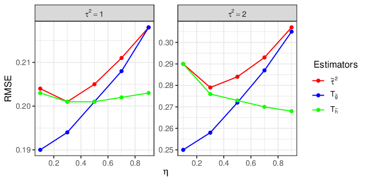
Refer to caption
Figure 2: Root mean square error (RMSE) for the proposed estimators. The x-axis stands for the sparsity level η\eta.
Table 2: Summary statistics for the EigenPrism-related estimators; n=p=300.n=p=300. Biases, standard errors (SE) and the root mean square errors (RMSE) of the different estimators, computed over 100100 independent datasets for each setting. The relative improvement over the EigenPrism estimator τ~2\tilde{\tau}^{2} (in terms of RMSE) is also shown. An estimate for the standard deviation of RMSE (σ^R​M​S​E\hat{\sigma}_{RMSE}) was calculated using the delta method.
η\eta τ2\tau^{2} Estimator Bias SE RMSE % Change σ^R​M​S​E\hat{\sigma}_{RMSE}
10% 1 τ~2\tilde{\tau}^{2} 0.01 0.204 0.204 0.00 0.014
10% 1 Tg~T_{\tilde{g}} 0.01 0.19 0.19 -6.86 0.012
10% 1 Th~T_{\tilde{h}} 0.01 0.204 0.203 -0.49 0.014
30% 1 τ~2\tilde{\tau}^{2} 0.01 0.202 0.201 0.00 0.014
30% 1 Tg~T_{\tilde{g}} 0.01 0.195 0.194 -3.48 0.014
30% 1 Th~T_{\tilde{h}} 0.01 0.201 0.201 0.00 0.014
50% 1 τ~2\tilde{\tau}^{2} 0.00 0.206 0.205 0.00 0.014
50% 1 Tg~T_{\tilde{g}} 0.00 0.202 0.201 -1.95 0.014
50% 1 Th~T_{\tilde{h}} 0.01 0.202 0.201 -1.95 0.015
70% 1 τ~2\tilde{\tau}^{2} 0.00 0.212 0.211 0.00 0.015
70% 1 Tg~T_{\tilde{g}} 0.00 0.209 0.208 -1.42 0.015
70% 1 Th~T_{\tilde{h}} 0.00 0.203 0.202 -4.27 0.015
90% 1 τ~2\tilde{\tau}^{2} -0.01 0.219 0.218 0.00 0.016
90% 1 Tg~T_{\tilde{g}} -0.01 0.218 0.218 0.00 0.016
90% 1 Th~T_{\tilde{h}} 0.00 0.204 0.203 -6.88 0.015
10% 2 τ~2\tilde{\tau}^{2} 0.00 0.291 0.29 0.00 0.020
10% 2 Tg~T_{\tilde{g}} 0.02 0.251 0.25 -13.79 0.016
10% 2 Th~T_{\tilde{h}} 0.01 0.291 0.29 0.00 0.020
30% 2 τ~2\tilde{\tau}^{2} 0.03 0.279 0.279 0.00 0.019
30% 2 Tg~T_{\tilde{g}} 0.03 0.258 0.258 -7.53 0.018
30% 2 Th~T_{\tilde{h}} 0.03 0.276 0.276 -1.08 0.019
50% 2 τ~2\tilde{\tau}^{2} 0.02 0.285 0.284 0.00 0.019
50% 2 Tg~T_{\tilde{g}} 0.01 0.273 0.272 -4.23 0.019
50% 2 Th~T_{\tilde{h}} 0.02 0.274 0.273 -3.87 0.020
70% 2 τ~2\tilde{\tau}^{2} 0.01 0.294 0.293 0.00 0.020
70% 2 Tg~T_{\tilde{g}} 0.00 0.289 0.287 -2.05 0.019
70% 2 Th~T_{\tilde{h}} 0.01 0.271 0.27 -7.85 0.019
90% 2 τ~2\tilde{\tau}^{2} -0.01 0.308 0.307 0.00 0.022
90% 2 Tg~T_{\tilde{g}} -0.01 0.307 0.305 -0.65 0.022
90% 2 Th~T_{\tilde{h}} 0.00 0.269 0.268 -12.7 0.019

7 Discussion and Future Work

In this work, we proposed a zero-estimator approach for improving estimation of the signal and noise levels explained by a set of covariates in a high-dimensional regression setting when the covariate distribution is known. We presented theoretical properties of the naive estimator τ^2,\hat{\tau}^{2}, and the proposed improved estimators Th^T_{\hat{h}} and Tg^T_{\hat{g}}. In a simulation study, we demonstrated that the zero-estimator approach leads to a significant reduction in the RMSE. Our method does not rely on sparsity assumptions of the regression coefficient vector, normality of the covariates, or linearity of E⁡(Y|X)E(Y|X). The goal in this work is to estimate the signal coming from the best linear function of the covariates, which is a model-free quantity. Our simulations demonstrate that our approach can be generalized to improve other estimators as well.

We suggest the following directions for future work. One natural extension is to relax the assumption of known covariate distribution to allow for a more general setting. This may be studied under the semi-supervised setting where one has access to a large amount of unlabeled data (N≫nN\gg n) in order to obtain theoretical results as a function of N.N. Another possible future research might be to extend the proposed approach to generalized linear models (GLM) such as logistic and Poisson regression, or survival models.

References

  • Azriel (2019) Azriel, D. (2019). The conditionality principle in high-dimensional regression. Biometrika 106(3), 702–707.
  • Berrett et al. (2020) Berrett, T. B., Y. Wang, R. F. Barber, and R. J. Samworth (2020). The conditional permutation test for independence while controlling for confounders. Journal of the Royal Statistical Society: Series B (Statistical Methodology) 82(1), 175–197.
  • Bonnet et al. (2015) Bonnet, A., E. Gassiat, and C. Lévy-Leduc (2015). Heritability estimation in high dimensional sparse linear mixed models. Electronic Journal of Statistics 9(2), 2099–2129.
  • Bose and Chatterjee (2018) Bose, A. and S. Chatterjee (2018). U-statistics, Mm-estimators and Resampling. Springer.
  • Buja et al. (2019) Buja, A., L. Brown, A. K. Kuchibhotla, R. Berk, E. George, and L. Zhao (2019). Models as approximations ii: A model-free theory of parametric regression. Statistical Science 34(4), 545–565.
  • Cai and Guo (2020) Cai, T. and Z. Guo (2020). Semisupervised inference for explained variance in high dimensional linear regression and its applications. Journal of the Royal Statistical Society: Series B (Statistical Methodology).
  • Candes et al. (2018) Candes, E., Y. Fan, L. Janson, and J. Lv (2018). Panning for gold:‘model-x’knockoffs for high dimensional controlled variable selection. Journal of the Royal Statistical Society: Series B (Statistical Methodology) 80(3), 551–577.
  • Chatterjee and Jafarov (2015) Chatterjee, S. and J. Jafarov (2015). Prediction error of cross-validated lasso. arXiv preprint arXiv:1502.06291.
  • Chen (2022) Chen, H. Y. (2022). Statistical inference on explained variation in high-dimensional linear model with dense effects. arXiv preprint arXiv:2201.08723.
  • de Los Campos et al. (2015) de Los Campos, G., D. Sorensen, and D. Gianola (2015). Genomic heritability: what is it? PLoS Genetics 11(5), e1005048.
  • Dicker (2014) Dicker, L. H. (2014). Variance estimation in high-dimensional linear models. Biometrika 101(2), 269–284.
  • Fan et al. (2012) Fan, J., S. Guo, and N. Hao (2012). Variance estimation using refitted cross-validation in ultrahigh dimensional regression. Journal of the Royal Statistical Society: Series B (Statistical Methodology) 74(1), 37–65.
  • Glynn and Szechtman (2002) Glynn, P. W. and R. Szechtman (2002). Some new perspectives on the method of control variates. In Monte Carlo and Quasi-Monte Carlo Methods 2000, pp. 27–49. Springer.
  • Hansen (2022) Hansen, B. E. (2022). Econometrics. Princeton University Press.
  • Hastie et al. (2015) Hastie, T., R. Tibshirani, and M. Wainwright (2015). Statistical learning with sparsity the lasso and generalizations. Chapman amp.
  • Janson et al. (2017) Janson, L., R. F. Barber, and E. Candes (2017). Eigenprism: inference for high dimensional signal-to-noise ratios. Journal of the Royal Statistical Society: Series B (Statistical Methodology) 79(4), 1037–1065.
  • Kong and Valiant (2018) Kong, W. and G. Valiant (2018). Estimating learnability in the sublinear data regime. Advances in Neural Information Processing Systems 31, 5455–5464.
  • Lavenberg and Welch (1981) Lavenberg, S. S. and P. D. Welch (1981). A perspective on the use of control variables to increase the efficiency of monte carlo simulations. Management Science 27(3), 322–335.
  • Livne et al. (2021) Livne, I., D. Azriel, and Y. Goldberg (2021). Improved estimators for semi-supervised high-dimensional regression model.
  • Oda et al. (2020) Oda, R., H. Yanagihara, et al. (2020). A fast and consistent variable selection method for high-dimensional multivariate linear regression with a large number of explanatory variables. Electronic Journal of Statistics 14(1), 1386–1412.
  • Sun and Zhang (2012) Sun, T. and C.-H. Zhang (2012). Scaled sparse linear regression. Biometrika 99(4), 879–898.
  • van der Vaart (2000) van der Vaart, A. W. (2000). Asymptotic statistics. Cambridge university press.
  • Verzelen et al. (2018) Verzelen, N., E. Gassiat, et al. (2018). Adaptive estimation of high-dimensional signal-to-noise ratios. Bernoulli 24(4B), 3683–3710.
  • Wang and Janson (2020) Wang, W. and L. Janson (2020). A power analysis of the conditional randomization test and knockoffs. arXiv preprint arXiv:2010.02304.
  • Yang et al. (2010) Yang, J., B. Benyamin, B. P. McEvoy, S. Gordon, A. K. Henders, D. R. Nyholt, P. A. Madden, A. C. Heath, N. G. Martin, G. W. Montgomery, et al. (2010). Common snps explain a large proportion of the heritability for human height. Nature genetics 42(7), 565–569.
  • Young (2022) Young, A. I. (2022). Discovering missing heritability in whole-genome sequencing data. Nature Genetics, 1–2.
  • Zhang and Bradic (2019) Zhang, Y. and J. Bradic (2019). High-dimensional semi-supervised learning: in search for optimal inference of the mean. arXiv preprint arXiv:1902.00772.
  • Zhu and Zhou (2020) Zhu, H. and X. Zhou (2020). Statistical methods for snp heritability estimation and partition: a review. Computational and Structural Biotechnology Journal 18, 1557–1568.

8 Appendix

Proof of Proposition 1.


Let Wi=(Wi​1,…,Wi​p)T{W_{i}}={\left({{W_{i1}},...,{W_{ip}}}\right)^{T}} and notice that τ^2=1n⁡(n−1)​∑i1≠i2n∑j=1pWi1​j​Wi2​j\hat{\tau}^{2}=\frac{1}{{n\left({n-1}\right)}}\sum\limits_{{i_{1}}\neq{i_{2}}}^{n}\sum\limits_{j=1}^{p}{{W_{{i_{1}}j}}{W_{{i_{2}}j}}} is a U-statistic of order 2 with the kernel hτ​(W1,W2)=W1T​W2=∑j=1pW1​j​W2​j.h_{\tau}\left({{W_{1}},{W_{2}}}\right)=W_{1}^{T}{W_{2}}=\sum\limits_{j=1}^{p}{{W_{1j}}{W_{2j}}}.

By Theorem 12.3 in van der Vaart 2000,

Var​(τ^2)=4​(n−2)n⁡(n−1)​ζ1+2n⁡(n−1)​ζ2,{\text{Var}}\left({{{\hat{\tau}}^{2}}}\right)=\frac{{4\left({n-2}\right)}}{{n\left({n-1}\right)}}{\zeta_{1}}+\frac{2}{{n\left({n-1}\right)}}{\zeta_{2}}, (22)

where ζ1≡Cov​[h⁡(W1,W2),h⁡(W1,W~2)]{\zeta_{1}}\equiv{\text{Cov}}\left[{h\left({{W_{1}},{W_{2}}}\right),h\left({{W_{1}},{{\widetilde{W}_{2}}}}\right)}\right] and ζ2≡Var​[h⁡(W1,W2)],{\zeta_{2}}\equiv{\text{Var}}\left[{h\left({{W_{1}},{W_{2}}}\right)}\right], and where W~2\widetilde{W}_{2} is an independent copy of W2W_{2}. Define the p×pp\times p matrix 𝐀=E⁡(W​WT){\bf{A}}=E\left({{{W}}{W}^{T}}\right) and notice that

ζ1\displaystyle{\zeta_{1}} ≡Cov​[h⁡(W1,W2),h⁡(W1,W~2)]\displaystyle\equiv\text{Cov}\left[{h\left({{{W}_{1}},{{W}_{2}}}\right),h\left({{{W}_{1}},{{\widetilde{W}}_{2}}}\right)}\right]
=∑j,j′pCov​(W1​j​W2​j,W1​j′​W~2​j′)=∑j,j′p(βj​βj′​E​[W1​j​W1​j′]−βj2​βj′2)\displaystyle=\sum\limits_{j,j^{\prime}}^{p}{\text{Cov}\left({{W_{1j}}{W_{2j}},{W_{1j^{\prime}}}{{\widetilde{W}}_{2j^{\prime}}}}\right)}=\sum\limits_{j,j^{\prime}}^{p}{\left({{\beta_{j}}{\beta_{j^{\prime}}}E\left[{{W_{1j}}{W_{1j^{\prime}}}}\right]-\beta_{j}^{2}\beta_{j^{\prime}}^{2}}\right)}
=βT​𝐀​β−‖β‖4,\displaystyle={\beta^{T}}{\bf{A}}\beta-{\left\|\beta\right\|^{4}},

and

ζ2\displaystyle{\zeta_{2}} ≡Cov​[h⁡(W1,W2),h⁡(W1,W2)]\displaystyle\equiv{\text{Cov}}\left[{h\left({{{W}_{1}},{{W}_{2}}}\right),h\left({{{W}_{1}},{{W}_{2}}}\right)}\right]
=∑j,j′Cov​(W1​j​W2​j,W1​j′​W2​j′)=∑j,j′((E⁡[W1​j​W1​j′])2−βj2​βj′2)\displaystyle=\sum\limits_{j,j^{\prime}}{{\text{Cov}}\left({{W_{1j}}{W_{2j}},{W_{1j^{\prime}}}{W_{2j^{\prime}}}}\right)}=\sum\limits_{j,j^{\prime}}\left({{{\left({E\left[{{W_{1j}}{W_{1j^{\prime}}}}\right]}\right)}^{2}}-\beta_{j}^{2}\beta_{j^{\prime}}^{2}}\right)
=‖𝐀‖F2−‖β‖4,\displaystyle=\left\|{\bf{A}}\right\|_{F}^{2}-{\left\|\beta\right\|^{4}},

where ‖A‖F2\|\textbf{A}\|_{F}^{2} is the Frobenius norm of A.\textbf{A}. Thus, (7) follows from (22). ∎

Proof of Proposition 2.


Since τ^2\hat{\tau}^{2} is an unbiased estimator of τ2,\tau^{2}, then it is enough to prove that Var​[τ^2]→n→∞0\text{Var}[\hat{\tau}^{2}]\xrightarrow{n\rightarrow\infty}0. By (7) it is enough to require that βT​A​βn→n→∞0\frac{\beta^{T}\textbf{A}\beta}{n}\xrightarrow{n\rightarrow\infty}0 and ‖A‖F2n2→n→∞0\frac{\|\textbf{A}\|^{2}_{F}}{n^{2}}\xrightarrow{n\rightarrow\infty}0. The latter is assumed and we now show that the former also holds true.
Let λ1​𝐀≥…≥λp​𝐀\lambda_{1{\bf A}}\geq...\geq\lambda_{p{\bf A}} be the eigenvalues of A and notice that A is symmetric. Thus,

1n2​(λ1​𝐀)2≤1n2​∑j=1pλj​𝐀2=1n2​t​r​(A2)=1n2​‖A‖F2.\frac{1}{n^{2}}(\lambda_{1{\bf A}})^{2}\leq\frac{1}{n^{2}}\sum_{j=1}^{p}\lambda_{j{\bf A}}^{2}=\frac{1}{n^{2}}tr(\textbf{A}^{2})=\frac{1}{n^{2}}\|\textbf{A}\|_{F}^{2}.

Since we assume that ‖A‖F2n2→n→∞0\frac{\|\textbf{A}\|^{2}_{F}}{n^{2}}\xrightarrow{n\rightarrow\infty}0, we can conclude that λ1​𝐀n→n→∞0\frac{\lambda_{1{\bf A}}}{n}\xrightarrow{n\rightarrow\infty}0. Now, recall that the maximum of the quadratic form aT​𝐀​a{a^{T}}{\bf{A}}a satisfies λ1​𝐀=maxaaT​𝐀​a‖a‖2.{\lambda_{1{\bf A}}}=\mathop{\max}\limits_{a}\,\frac{{{a^{T}}{\bf{A}}a}}{{{{\left\|a\right\|}^{2}}}}. Hence,

1n​βT​A​β≡1n​‖β‖2​[(β‖β‖)T​A​β‖β‖]≤1n​‖β‖2​λ1=λ1n​τ2→n→∞0,\frac{1}{n}\beta^{T}\textbf{A}\beta\equiv\frac{1}{n}\|\beta\|^{2}[(\frac{\beta}{\|\beta\|})^{T}\textbf{A}\frac{\beta}{\|\beta\|}]\leq\frac{1}{n}\|\beta\|^{2}\lambda_{1}=\frac{\lambda_{1}}{n}\tau^{2}\xrightarrow{n\rightarrow\infty}0,

where the last limit follows from the assumption that τ2=O⁡(1),\tau^{2}=O(1), and from the fact that λ1n→n→∞0.\frac{\lambda_{1}}{n}\xrightarrow{n\rightarrow\infty}0.
We conclude that Var​[τ^2]→n→∞0\text{Var}[\hat{\tau}^{2}]\xrightarrow{n\rightarrow\infty}0. ∎

Proof of Proposition 3.


Recall that (8) states that σ^2≡σ^Y2−τ^2{\hat{\sigma}^{2}}\equiv\hat{\sigma}_{Y}^{2}-{\hat{\tau}^{2}}. Thus,

Var​(σ^2)=Var​(τ^2)+Var​(σ^Y2)−2​Cov​(σ^Y2,τ^2).\displaystyle\text{Var}\left({{{\hat{\sigma}}^{2}}}\right)=\text{Var}\left({{{\hat{\tau}}^{2}}}\right)+\text{Var}\left({\hat{\sigma}_{Y}^{2}}\right)-2\text{Cov}\left(\hat{\sigma}_{Y}^{2},{\hat{\tau}}^{2}\right). (23)

The variance of τ^2\hat{\tau}^{2} is given in (7). By standard U-statistic calculations (see e.g., Example 1.8 in Bose and Chatterjee 2018), the variance of σ^Y2\hat{\sigma}_{Y}^{2} is

Var​(σ^Y2)=4​(n−2)n⁡(n−1)​ψ1+2n⁡(n−1)​ψ2,\displaystyle\text{Var}(\hat{\sigma}_{Y}^{2})=\frac{4(n-2)}{n(n-1)}\psi_{1}+\frac{2}{n(n-1)}\psi_{2},

where ψ1≡μ4−σY44\psi_{1}\equiv\frac{\mu_{4}-\sigma_{Y}^{4}}{4} and ψ2≡μ4+σY42.\psi_{2}\equiv\frac{\mu_{4}+\sigma_{Y}^{4}}{2}. This can be further simplified to obtain

Var​(σ^Y2)=1n​μ4−(n−3)n⁡(n−1)​σY4.\displaystyle\text{Var}\left({\hat{\sigma}_{Y}^{2}}\right)=\frac{1}{n}{\mu_{4}}-\frac{{\left({n-3}\right)}}{{n\left({n-1}\right)}}\sigma_{Y}^{4}. (24)

We now calculate the covariance between and σ^Y2\hat{\sigma}_{Y}^{2} and τ^2.\hat{\tau}^{2}. Write,

Cov​(σ^Y2,τ^2)=Cov​[1n⁡(n−1)​∑i1≠i2(Yi1−Yi2)2/2,1n⁡(n−1)​∑j=1p∑i1≠i2Wi1​j​Wi2​j]\displaystyle\text{Cov}\left({\hat{\sigma}_{Y}^{2},{{\hat{\tau}}^{2}}}\right)=\text{Cov}\left[{\frac{1}{{n\left({n-1}\right)}}\sum\limits_{{i_{1}}\neq{i_{2}}}{{{\left({{Y_{{i_{1}}}}-{Y_{{i_{2}}}}}\right)}^{2}}/2,\frac{1}{{n\left({n-1}\right)}}\sum\limits_{j=1}^{p}{\sum\limits_{{i_{1}}\neq{i_{2}}}{{W_{{i_{1}}j}}{W_{{i_{2}}j}}}}}}\right]
=12​n2​(n−1)2​∑j=1p∑i1≠i2∑i3≠i4Cov​[Wi3​j​Wi4​j,(Yi1−Yi2)2].\displaystyle=\frac{1}{{2{n^{2}}{{\left({n-1}\right)}^{2}}}}\sum\limits_{j=1}^{p}{\sum\limits_{{i_{1}}\neq{i_{2}}}{\sum\limits_{{i_{3}}\neq{i_{4}}}{\text{Cov}\left[{{W_{{i_{3}}j}}{W_{{i_{4}}j}}},{{\left({{Y_{{i_{1}}}}-{Y_{{i_{2}}}}}\right)}^{2}}\right]}}}.

The covariance above is different from zero either when one of {i1,i2}\{i_{1},i_{2}\} is equal to one of {i3,i4}\{i_{3},i_{4}\}, or when {i1,i2}\{i_{1},i_{2}\} is equal to {i3,i4}\{i_{3},i_{4}\}. There are 4​n​(n−1)​(n−2)4n(n-1)(n-2) quadruples (i1,i2,i3,i4)(i_{1},i_{2},i_{3},i_{4}) for the first case, and 2​n​(n−1)2n(n-1) for the second case. Therefore,

Cov​[σ^Y2,τ^2]=2​(n−2)n⁡(n−1)​∑j=1pCov​[W1​j​W2​j,(Y−Y3)2]+1n⁡(n−1)​∑j=1pCov​[W1​j​W2​j,(Y1−Y2)2].\displaystyle\text{Cov}[\hat{\sigma}_{Y}^{2},\hat{\tau}^{2}]=\frac{2(n-2)}{n(n-1)}\sum_{j=1}^{p}\text{Cov}[W_{1j}{W_{2j}},(Y-Y_{3})^{2}]+\frac{1}{n(n-1)}\sum_{j=1}^{p}\text{Cov}[W_{1j}W_{2j},(Y_{1}-{Y_{2}})^{2}]. (25)

The first covariance term in (25) is

Cov​[W1​j​W2​j,(Y1−Y3)2]=E⁡([W1​j​W2​j−E⁡(W1​j)​E​(W2​j)]​[(Y1−Y3)2−2​σY2])\displaystyle\text{Cov}[W_{1j}W_{2j},(Y_{1}-Y_{3})^{2}]=E\Big([W_{1j}W_{2j}-E(W_{1j})E(W_{2j})][(Y_{1}-Y_{3})^{2}-2\sigma_{Y}^{2}]\Big)
=E⁡([W1​j​W2​j−βj2]​[(Y1−α−(Y3−α))2−2​σY2])\displaystyle=E\Big([W_{1j}W_{2j}-\beta_{j}^{2}][(Y_{1}-\alpha-(Y_{3}-\alpha))^{2}-2\sigma_{Y}^{2}]\Big)
=E⁡([W1​j​W2​j−βj2]​[{(Y1−α)2−σY2}−2​(Y1−α)​(Y3−α)+(Y3−α)2−σY2])\displaystyle=E\Big([W_{1j}W_{2j}-\beta_{j}^{2}][\{(Y_{1}-\alpha)^{2}-\sigma_{Y}^{2}\}-2(Y_{1}-\alpha)(Y_{3}-\alpha)+(Y_{3}-\alpha)^{2}-\sigma_{Y}^{2}]\Big)
=E⁡([W1​j​W2​j−βj2]​[{(Y1−α)2−σY2}])\displaystyle=E\Big([W_{1j}W_{2j}-\beta_{j}^{2}][\{(Y_{1}-\alpha)^{2}-\sigma_{Y}^{2}\}]\Big)
=E⁡[W1​j​(Y1−α)2]​βj2−βj2​σY2.\displaystyle=E\left[{{W_{1j}}{{\left({Y_{1}-\alpha}\right)}^{2}}}\right]\beta_{j}^{2}-\beta_{j}^{2}\sigma_{Y}^{2}.

The second covariance term of (25) is

Cov​[W1​j​W2​j,(Y1−Y2)2]=E⁡{[W1​j​W2​j−E⁡(W1​j​W2​j)]​[(Y1−Y2)2−E⁡{(Y1−Y2)2}]}\displaystyle\text{Cov}\left[{W_{1j}W_{2j},{{\left(Y_{1}-Y_{2}\right)}^{2}}}\right]=E\left\{{\left[{W_{1j}W_{2j}-E\left({W_{1j}W_{2j}}\right)}\right]\left[{{{\left(Y_{1}-Y_{2}\right)}^{2}}-E\left\{{{{\left(Y_{1}-Y_{2}\right)}^{2}}}\right\}}\right]}\right\}
=E⁡{(W1​j​W2​j−βj2)​[(Y1−Y2)2−2​σY2]}\displaystyle=E\left\{{\left({W_{1j}W_{2j}-\beta_{j}^{2}}\right)\left[{{{\left(Y_{1}-Y_{2}\right)}^{2}}-2\sigma_{Y}^{2}}\right]}\right\}
=E⁡{(W1​j​W2​j−βj2)​[{(Y1−α)−(Y2−α)}2−2​σY2]}\displaystyle=E\left\{{\left({W_{1j}W_{2j}-\beta_{j}^{2}}\right)\left[{{{\left\{{\left({Y_{1}-\alpha}\right)-\left({Y_{2}-\alpha}\right)}\right\}}^{2}}-2\sigma_{Y}^{2}}\right]}\right\}
=E⁡{(W1​j​W2​j−βj2)​[{(Y1−α)2−σY2}−2​(Y1−α)​(Y2−α)+{(Y2−α)2−σY2}]}\displaystyle=E\left\{{\left({W_{1j}W_{2j}-\beta_{j}^{2}}\right)\left[{\left\{{{{\left({Y_{1}-\alpha}\right)}^{2}}-\sigma_{Y}^{2}}\right\}-2\left({Y_{1}-\alpha}\right)\left({Y_{2}-\alpha}\right)+\left\{{{{\left({Y_{2}-\alpha}\right)}^{2}}-\sigma_{Y}^{2}}\right\}}\right]}\right\}
=2​E​{[(Y1−α)2−σY2]​(W1​j​W2​j−βj2)}−2​E​[(W1​j​W2​j−βj2)​(Y1−α)​(Y2−α)]\displaystyle=2E\left\{{\left[{{{\left({Y_{1}-\alpha}\right)}^{2}}-\sigma_{Y}^{2}}\right]\left({W_{1j}W_{2j}-\beta_{j}^{2}}\right)}\right\}-2E\left[{\left({W_{1j}W_{2j}-\beta_{j}^{2}}\right)\left({Y_{1}-\alpha}\right)\left({Y_{2}-\alpha}\right)}\right]
=2​{E⁡[(Y1−α)2​W1​j]​βj−σY2​βj2}−2​E​[W1​j​(Y1−α)​W2​j​(Y2−α)]\displaystyle=2\left\{{E\left[{{{\left({Y_{1}-\alpha}\right)}^{2}}{W_{1j}}}\right]{\beta_{j}}-\sigma_{Y}^{2}\beta_{j}^{2}}\right\}-2E\left[{{W_{1j}}\left({Y_{1}-\alpha}\right)W_{2j}\left({Y_{2}-\alpha}\right)}\right]
=2​E​[(Y1−α)2​W1​j]​βj−2​σY2​βj2−2​{E⁡[W1​j​(Y1−α)]}2,\displaystyle=2E\left[{{{\left({Y_{1}-\alpha}\right)}^{2}}{W_{1j}}}\right]{\beta_{j}}-2\sigma_{Y}^{2}\beta_{j}^{2}-2{\left\{{E\left[{{W_{1j}}\left({Y_{1}-\alpha}\right)}\right]}\right\}^{2}},

Hence, by (25) we have

Cov​(σ^Y2,τ^2)\displaystyle\text{Cov}\left({\hat{\sigma}_{Y}^{2},{{\hat{\tau}}^{2}}}\right) =2​(n−2)n⁡(n−1)​∑j=1p{E⁡[W1​j​(Y1−α)2]​βj−βj2​σY2}\displaystyle=\frac{{2\left({n-2}\right)}}{{n\left({n-1}\right)}}\sum\limits_{j=1}^{p}{\left\{{E\left[{W_{1j}{{\left({Y_{1}-\alpha}\right)}^{2}}}\right]{\beta_{j}}-\beta_{j}^{2}\sigma_{Y}^{2}}\right\}}
+1n⁡(n−1)∑j=1p{2E[(Y1−α)2W1​j]βj−2σY2βj2−2{E[W1​j(Y1−α)]}2},\displaystyle+\frac{1}{{n\left({n-1}\right)}}\sum\limits_{j=1}^{p}{\left\{{2E\left[{{{\left({Y_{1}-\alpha}\right)}^{2}}W_{1j}}\right]{\beta_{j}}-2\sigma_{Y}^{2}\beta_{j}^{2}-2{{\left\{{E\left[{W_{1j}\left({Y_{1}-\alpha}\right)}\right]}\right\}}^{2}}}\right\}},

which can be further simplified as

Cov​(σ^Y2,τ^2)=2n​(πT​β−τ2​σY2)−2n⁡(n−1)​∑j=1p{E⁡[W1​j​(Y1−α)]}2,\displaystyle\text{Cov}\left({\hat{\sigma}_{Y}^{2},{{\hat{\tau}}^{2}}}\right)=\frac{2}{n}\left({{\pi^{T}}\beta-{\tau^{2}}\sigma_{Y}^{2}}\right)-\frac{2}{{n\left({n-1}\right)}}\sum\limits_{j=1}^{p}{{{\left\{{E\left[{W_{1j}\left({Y_{1}-\alpha}\right)}\right]}\right\}}^{2}}}, (26)

where π=(π1,…,πp)T\pi={\left({{\pi_{1}},...,{\pi_{p}}}\right)^{T}} and πj≡E⁡[(Y1−α)2​W1​j]{\pi_{j}}\equiv E\left[{{{\left({Y_{1}-\alpha}\right)}^{2}}W_{1j}}\right].
Plugging (24) and (26) into (23) leads to (3). ∎

Proof of Corollary 1.


Since σ^2\hat{\sigma}^{2} is an unbiased estimator of σ2,\sigma^{2}, it is enough to prove that Var​(σ^2)→n→∞ 0.\text{Var}(\hat{\sigma}^{2})\xrightarrow{n\rightarrow\infty}\penalty\ 0. Recall that σ^2=σ^Y2−τ^2\hat{\sigma}^{2}=\hat{\sigma}^{2}_{Y}-\hat{\tau}^{2}. It follows that Var​(σ^2)≤2​Var​(σ^Y2)+2​Var​(τ^2)\text{Var}\left({{{\hat{\sigma}}^{2}}}\right)\leq 2\text{Var}\left({\hat{\sigma}_{Y}^{2}}\right)+2\text{Var}\left({{{\hat{\tau}}^{2}}}\right). Thus, it is enough to prove that Var​(σ^Y2)→n→∞ 0\text{Var}(\hat{\sigma}_{Y}^{2})\xrightarrow{n\rightarrow\infty}\penalty\ 0 and Var​(τ^2)→n→∞ 0.\text{Var}(\hat{\tau}^{2})\xrightarrow{n\rightarrow\infty}\penalty\ 0. The former requires, by (24), the assumption that μ4\mu_{4} is bounded and the latter holds true by Proposition 2. ∎

Remark 1.

The condition ‖𝐀‖F2n2→0\frac{\|{\bf A}\|_{F}^{2}}{n^{2}}\rightarrow 0 holds in the homoskedastic linear model with the additional assumption that the columns of 𝐗\bf{X} are independent (Livne et al. 2021, Proposition 2). We now show two more examples where the condition ‖𝐀‖F2n2→0\frac{\|{\bf A}\|_{F}^{2}}{n^{2}}\rightarrow 0 holds without assuming linearity.

1) We show that if p/n2→0p/n^{2}\rightarrow 0 and Y2≤CY^{2}\leq C for some constant CC, then ‖𝐀‖F2n2→0\frac{\|{\bf A}\|_{F}^{2}}{n^{2}}\rightarrow 0. For a∈ℝpa\in\mathbb{R}^{p} we have,

aT​𝐀​a\displaystyle{a^{T}}{\bf{A}}a =aT​E​(𝐖𝐖T)​a=E⁡(aT​𝐖𝐖T​a)=E⁡[(aT​𝐖)2]\displaystyle={a^{T}}E\left({{\bf{W}}{{\bf{W}}^{T}}}\right)a=E\left({{a^{T}}{\bf{W}}{{\bf{W}}^{T}}a}\right)=E\left[{{{\left({{a^{T}}{\bf{W}}}\right)}^{2}}}\right]
=E⁡[(Y​∑j=1paj​Xi​j)2]≤C​E​[(∑j=1paj​Xi​j)2]\displaystyle=E\left[{{{\left(Y{\sum\limits_{j=1}^{p}{{a_{j}}{X_{ij}}}}\right)}^{2}}}\right]\leq{C}E\left[{{{\left({\sum\limits_{j=1}^{p}{{a_{j}}{X_{ij}}}}\right)}^{2}}}\right]
=C⁡{∑j=1paj2​E⁡(Xi​j2)⏟1}+C​E​(∑j≠j′aj​aj′​E⁡(Xi​j​Xj′)⏟0)\displaystyle={C}\left\{{\sum\limits_{j=1}^{p}{a_{j}^{2}\underbrace{E\left({X_{ij}^{2}}\right)}_{1}}}\right\}+CE\left({\sum\limits_{j\neq j^{\prime}}{{a_{j}}{a_{j^{\prime}}}}\underbrace{E\left({{X_{ij}}{X_{j^{\prime}}}}\right)}_{0}}\right)
=C​‖a‖2,\displaystyle={C}{\left\|a\right\|^{2}}, (27)

where the last equality follows from Σ=𝐈.{\Sigma}={\bf I}. Now, let λ1​𝐀≥λ2𝐀≥,…,≥λp​𝐀𝐀\lambda_{1{\bf A}}\geq\lambda_{2}^{\bf A}\geq,...,\geq\lambda_{p{\bf A}}^{\bf A} be the eigenvalues of 𝐀,\bf{A}, and recall that the extrema of the quadratic form aT​𝐀​a{a^{T}}{\bf{A}}a satisfies λ1​𝐀=maxaaT​𝐀​a‖a‖2,{\lambda_{1{\bf A}}}=\mathop{\max}\limits_{a}\,\frac{{{a^{T}}{\bf{A}}a}}{{{{\left\|a\right\|}^{2}}}}, and hence by (1) we have λ1≤C.\lambda_{1}\leq C. Now, since p/n2→0p/n^{2}\rightarrow 0 by assumption, it follows that

‖𝐀‖F2n2=t​r​a​c​e​(𝐀2)n2=∑j=1pλj​𝐀2n2≤p​λ1​𝐀2n2≤p​C2n2→0.\frac{{\left\|{\bf{A}}\right\|_{F}^{2}}}{{{n^{2}}}}=\frac{{trace\left({{{\bf{A}}^{2}}}\right)}}{{{n^{2}}}}=\frac{{\sum\limits_{j=1}^{p}{\lambda_{j{\bf A}}^{2}}}}{{{n^{2}}}}\leq\frac{{p\lambda_{1{\bf A}}^{2}}}{{{n^{2}}}}\leq\frac{{p{C^{2}}}}{{{n^{2}}}}\to 0. (28)

2) We show that if p/n2→0p/n^{2}\rightarrow 0, E⁡(Y4),E⁡(Xi​j4)≤CE(Y^{4}),E(X_{ij}^{4})\leq C for j=1,…,pj=1,...,p and C≥1C\geq 1, and the columns of 𝐗\bf{X} are independent, then ‖𝐀‖F2n2→0\frac{\|{\bf A}\|_{F}^{2}}{n^{2}}\rightarrow 0. For a∈ℝpa\in\mathbb{R}^{p} we have by Cauchy–Schwarz,

aT​𝐀​a\displaystyle{a^{T}}{\bf{A}}a =E⁡[Yi2​(∑j=1paj​Xi​j)2]≤[E⁡(Yi4)]1/2​{E⁡[(∑j=1paj​Xi​j)4]}1/2\displaystyle=E\left[{Y_{i}^{2}{{\left({\sum\limits_{j=1}^{p}{{a_{j}}{X_{ij}}}}\right)}^{2}}}\right]\leq{\left[{E\left({Y_{i}^{4}}\right)}\right]^{1/2}}{\left\{{E\left[{{{\left({\sum\limits_{j=1}^{p}{{a_{j}}{X_{ij}}}}\right)}^{4}}}\right]}\right\}^{1/2}}
≤C1/2​{∑j1​j2​j3​j4aj1​aj2​aj3​aj4​E​(Xi​j1​Xi​j2​Xi​j3​Xi​j4)}1/2\displaystyle\leq{C^{1/2}}{\left\{{\sum\limits_{{j_{1}}{j_{2}}{j_{3}}{j_{4}}}{{a_{{j_{1}}}}{a_{{j_{2}}}}{a_{{j_{3}}}}{a_{{j_{4}}}}E\left({{X_{i{j_{1}}}}{X_{i{j_{2}}}}{X_{i{j_{3}}}}{X_{i{j_{4}}}}}\right)}}\right\}^{1/2}}
≤C1/2​{∑j=1paj4​E​(Xi​j4)+∑j≠j′aj2​aj′2​E​(Xi​j2)​E​(Xi​j′2)}1/2\displaystyle\leq{C^{1/2}}{\left\{{\sum\limits_{j=1}^{p}{a_{j}^{4}E\left({X_{ij}^{4}}\right)+\sum\limits_{j\neq j^{\prime}}{a_{j}^{2}a_{j^{\prime}}^{2}E\left({X_{ij}^{2}}\right)E\left({X_{ij^{\prime}}^{2}}\right)}}}\right\}^{1/2}}
≤C1/2​{C​∑j=1paj4+C​∑j≠j′aj2​aj′2}1/2\displaystyle\leq{C^{1/2}}{\left\{{C\sum\limits_{j=1}^{p}{a_{j}^{4}+C\sum\limits_{j\neq j^{\prime}}{a_{j}^{2}a_{j^{\prime}}^{2}}}}\right\}^{1/2}}
≤C​{∑j=1paj4+∑j≠j′aj2​aj′2}1/2=C​‖a‖2.\displaystyle\leq C{\left\{{\sum\limits_{j=1}^{p}{a_{j}^{4}+\sum\limits_{j\neq j^{\prime}}{a_{j}^{2}a_{j^{\prime}}^{2}}}}\right\}^{1/2}}=C{\left\|a\right\|^{2}}.

Notice that since that the columns of 𝐗\bf{X} are independent, the expectation E⁡(Xi​j1​Xi​j2​Xi​j3​Xi​j4)E\left({{X_{i{j_{1}}}}{X_{i{j_{2}}}}{X_{i{j_{3}}}}{X_{i{j_{4}}}}}\right) is not zero (up to permutation) when j1=j2j_{1}=j_{2} and j3=j4j_{3}=j_{4} or when j1=j2=j3=j4.j_{1}=j_{2}=j_{3}=j_{4}. Also notice we obtained the same result as in (1), and hence ‖𝐀‖F2n2→0\frac{\|{\bf A}\|_{F}^{2}}{n^{2}}\rightarrow 0 follows by the same arguments as in the previous example.

Remark 2.

Calculations for Equation 13:
Write,

Cov​(τ^2,Zg)\displaystyle\text{Cov}\left({{{\hat{\tau}}^{2}},Z_{g}}\right) =Cov​(1n⁡(n−1)​∑i1≠i2∑j=1pWi1​j​Wi2​j,1n​∑i=1ng⁡(Xi))\displaystyle=\text{Cov}\left({\frac{1}{{n\left({n-1}\right)}}\sum\limits_{{i_{1}}\neq{i_{2}}}{\sum\limits_{j=1}^{p}{{W_{{i_{1}}j}}{W_{{i_{2}}j}}}},\frac{1}{n}\sum\limits_{i=1}^{n}{g(X_{i})}}\right)
=1n2​(n−1)​∑i1≠i2∑j=1p∑i=1nE⁡(Wi1​j​Wi2​j​g​(Xi))\displaystyle=\frac{1}{{{n^{2}}\left({n-1}\right)}}\sum\limits_{{i_{1}}\neq{i_{2}}}{\sum\limits_{j=1}^{p}{\sum\limits_{i=1}^{n}{E\left({{W_{{i_{1}}j}}{W_{{i_{2}}j}}g(X_{i})}\right)}}}
=2n2​(n−1)​∑i1≠i2∑j=1pE⁡(Wi1​j​gi1)​E​(Wi2​j)\displaystyle=\frac{2}{{{n^{2}}\left({n-1}\right)}}\sum\limits_{{i_{1}}\neq{i_{2}}}{\sum\limits_{j=1}^{p}{E\left({{W_{{i_{1}}j}}{g_{{i_{1}}}}}\right)E\left({{W_{{i_{2}}j}}}\right)}}
=2n2​(n−1)​∑i1≠i2∑j=1pE⁡(Wi1​j​gi1)​βj\displaystyle=\frac{2}{{{n^{2}}\left({n-1}\right)}}\sum\limits_{{i_{1}}\neq{i_{2}}}{\sum\limits_{j=1}^{p}{E\left({{W_{{i_{1}}j}}{g_{{i_{1}}}}}\right){\beta_{j}}}}
=2n​βT​θg,\displaystyle=\frac{2}{n}\beta^{T}\theta_{g},

where θg=E⁡[W​g​(X)]{\theta_{g}}=E\left[{Wg\left(X\right)}\right]. Also notice that Var​(Zg)=Var​(1n​∑i=1ng⁡(Xi))=Var​(g​(X))n.\text{Var}\left(Z_{g}\right)=\text{Var}\left({\frac{1}{n}\sum\limits_{i=1}^{n}{g(X_{i})}}\right)=\frac{{\text{Var}\left({g(X)}\right)}}{n}. Thus, by (11) we get

cg∗=Cov​(τ^2,Zg)Var​(Zg)=2​βT​θgVar​(g​(X)).{c_{g}^{*}}=\frac{{{\text{Cov}}\left({{{\hat{\tau}}^{2}},Z_{g}}\right)}}{{\text{Var}\left({Z_{g}}\right)}}=\frac{2\beta^{T}\theta_{g}}{{\text{Var}\left({g(X)}\right)}}.
Proof of Proposition 4.


We wish to prove that n​[Th−Th^]​→𝑝​ 0.\sqrt{n}\left[T_{h}-T_{\hat{h}}\right]\overset{p}{\rightarrow}\penalty\ 0. Write,

n​(Th−Th^)=n​[(Th−Tf)+(Tf−Tf^)+(Tf^−Th^)].\sqrt{n}\left({{T_{h}}-{T_{\hat{h}}}}\right)=\sqrt{n}\left[{\left({{T_{h}}-{T_{f}}}\right)+\left({{T_{f}}-{T_{\hat{f}}}}\right)+\left({{T_{\hat{f}}}-{T_{\hat{h}}}}\right)}\right].

Thus, we need to show that

n​(Th−Tf)​→𝑝​0,\displaystyle\sqrt{n}\left({T_{h}-T_{f}}\right)\overset{p}{\rightarrow}0, (29)
n​(Tf^−Th^)​→𝑝​ 0,and\displaystyle\sqrt{n}\left({T_{\hat{f}}-T_{\hat{h}}}\right)\overset{p}{\rightarrow}\penalty\ 0,\text{and} (30)
n​(Tf−Tf^)​→𝑝​0,\displaystyle\sqrt{n}\left({T_{f}-T_{\hat{f}}}\right)\overset{p}{\rightarrow}0, (31)

The proofs of (29) and (30) are essentially the same as the proof of Proposition 5 in Livne et al. 2021. This is true since h⁡(X)​𝟙A=f⁡(X)​𝟙A,h(X)\mathbbm{1}_{A}=f(X)\mathbbm{1}_{A}, where AA denotes the event that the selection procedure δ\delta perfectly selects the set Θ\Theta, i.e., A≡{𝐒δ=Θ},A\equiv\left\{{{{\bf{S}}_{\delta}}=\Theta}\right\}, and 𝟙A\mathbbm{1}_{A} denotes the indicator of A.A.

We now wish to prove (31). Write,

n​[Tf^−Tf]=n​[τ^2−c^f∗​Zf−(τ^2−cf∗​Zf)]=n​Zf​(cf∗−c^f∗).\sqrt{n}\left[T_{\hat{f}}-T_{f}\right]=\sqrt{n}\left[{{{\hat{\tau}}^{2}}-{\hat{c}_{f}^{*}}Z_{f}-\left({{{\hat{\tau}}^{2}}-{c_{f}^{*}}Z_{f}}\right)}\right]={\sqrt{n}}Z_{f}{\left({{{c_{f}^{*}}}-{\hat{c}_{f}^{*}}}\right)}.

By Markov and Cauchy-Schwarz inequalities, it is enough to show that

P{|nZf(c^f∗−cf∗)|>ε}≤E⁡{|n​Zf​(c^f∗−cf∗)|}ε≤n​E​(Zf2)​E​[(c^f∗−cf∗)2]ε→0.P\left\{{\left|{\sqrt{n}Z_{f}\left({\hat{c}_{f}^{*}-c_{f}^{*}}\right)}\right|>\varepsilon}\right\}\leq\frac{{E\left\{{\left|{\sqrt{n}Z_{f}\left({\hat{c}_{f}^{*}-c_{f}^{*}}\right)}\right|}\right\}}}{\varepsilon}\leq\frac{{\sqrt{nE\left({Z_{f}^{2}}\right)E\left[{{{\left({\hat{c}_{f}^{*}-c_{f}^{*}}\right)}^{2}}}\right]}}}{\varepsilon}\rightarrow 0.

Notice that E⁡(Zf2)=Var​(Zf)=Var​[f​(X)]nE(Z_{f}^{2})=\text{Var}(Z_{f})=\frac{\text{Var}[f(X)]}{n} and E⁡[(c^f∗−cf∗)2]=Var​(c^f∗),E[(\hat{c}_{f}^{*}-c_{f}^{*})^{2}]=\text{Var}(\hat{c}_{f}^{*}), where by (4) we have

c^f∗=2n⁡(n−1)​∑i1≠i2Wi1T​Wi2​f​(Xi2)Var​[f​(X)]≡UVar​[f​(X)].\hat{c}_{f}^{*}=\frac{{\frac{2}{{n\left({n-1}\right)}}\sum\limits_{{i_{1}}\neq{i_{2}}}{W_{{i_{1}}}^{T}{W_{{i_{2}}}}f\left({{X_{{i_{2}}}}}\right)}}}{{\text{Var}\left[{f\left(X\right)}\right]}}\equiv\frac{U}{\text{Var}[f(X)]}.

Hence, it enough to show that

Var​(U)Var​[f​(X)]→0.\frac{{\text{Var}\left(U\right)}}{{\text{Var}[f(X)]}}\rightarrow 0. (32)

The variance of UU is

Var​(U)\displaystyle\text{Var}(U) =Var​[2n⁡(n−1)​∑i1≠i2∑j=1pWi1​j​Wi2​j​f​(Xi2)]\displaystyle=\text{Var}\left[{\frac{2}{{n\left({n-1}\right)}}\sum\limits_{{i_{1}}\neq{i_{2}}}{\sum\limits_{j=1}^{p}{{W_{{i_{1}}j}}{W_{{i_{2}}j}}f(X_{i_{2}})}}}\right]
=4n2​(n−1)2​∑j,j′p∑i1≠i2,i3≠i4Cov​[Wi1​j​Wi2​j​f​(Xi2),Wi3​j′​Wi4​j′​f​(Xi4)].\displaystyle=\frac{4}{{{n^{2}}{{\left({n-1}\right)}^{2}}}}\sum\limits_{j,j^{\prime}}^{p}{\sum\limits_{{i_{1}}\neq{i_{2}},{i_{3}}\neq{i_{4}}}{\text{Cov}\left[{{W_{{i_{1}}j}}{W_{{i_{2}}j}}f(X_{i_{2}}),{W_{{i_{3}}j^{\prime}}}{W_{{i_{4}}j^{\prime}}}f(X_{i_{4}})}\right].}} (33)

The covariance in (8) is different from zero in the following two cases:

  1. 1.

    When {i1,i2}\left\{{{i_{1}},{i_{2}}}\right\} is equal to {i3,i4}.\left\{{{i_{3}},{i_{4}}}\right\}.

  2. 2.

    When one of {i1,i2}\left\{{{i_{1}},{i_{2}}}\right\} equals to {i3,i4}\left\{{{i_{3}},{i_{4}}}\right\} while the other is different.

The first condition includes two different sub-cases and each of those consists of n⁡(n−1)n(n-1) quadruples (i1,i2,i3,i4)(i_{1},i_{2},i_{3},i_{4}) that satisfy the condition. Similarly, the second condition above includes four different sub-cases and each of those consists of n​(n−1)​(n−2)n(n-1)(n-2) quadruples that satisfy the condition.

We now calculate the covariance for all these six sub-cases.
(1) The covariance when i1=i3,i2=i4{i_{1}}={i_{3}},{i_{2}}={i_{4}} is

Cov​[Wi1​j​Wi2​j​f​(Xi2),Wi1​j′​Wi2​j′​f​(Xi2)]\displaystyle\text{Cov}\left[{{W_{i_{1}j}}{W_{i_{2}j}}f(X_{i_{2}}),{W_{i_{1}j^{\prime}}}{{W_{i_{2}j^{\prime}}}}f(X_{i_{2}})}\right] =E⁡(Wi1​j​Wi1​j′)​E​[Wi2​j​Wi2​j′​f2​(Xi2)]\displaystyle=E\left({{W_{i_{1}j}}{W_{i_{1}j^{\prime}}}}\right)E\left[{{W_{i_{2}j}}{{W_{i_{2}j^{\prime}}}}f^{2}(X_{i_{2}})}\right]
−E⁡(Wi1​j)​E​[Wi2​j​f​(Xi2)]​E​(Wi1​j′)​E​[Wi2​j′​f​(Xi2)]\displaystyle-E({{W_{i_{1}j}}})E\left[{{W_{i_{2}j}}f(X_{i_{2}})}\right]E\left({{{W_{i_{1}j^{\prime}}}}}\right)E\left[{{{W_{i_{2}j^{\prime}}}}f(X_{i_{2}})}\right]
=E⁡(Wi1​j​Wi1​j′)​E​[Wi2​j​Wi2​j′​f2​(Xi2)]−βj​βj′​θf​j​θf​j′,\displaystyle=E\left({{W_{i_{1}j}}{W_{i_{1}j^{\prime}}}}\right)E\left[{{W_{i_{2}j}}{{W_{i_{2}j^{\prime}}}}f^{2}(X_{i_{2}})}\right]-{\beta_{j}}{\beta_{j^{\prime}}}{\theta_{fj}}{\theta_{fj^{\prime}}},

where recall that b≡W​f​(X).b\equiv Wf(X). Thus, we define

δ1≡∑j,j′{E⁡(Wi1​j​Wi1​j′)​E​[Wi2​j​Wi2​j′​f2​(Xi2)]−βj​βj′​θf​j​θf​j′}=E⁡(bT​𝐀​b)−(βT​θf)2.{\delta_{1}}\equiv\sum\limits_{j,j^{\prime}}{\left\{{E\left({{W_{i_{1}j}}{W_{i_{1}j^{\prime}}}}\right)E\left[{{W_{i_{2}j}}{W_{i_{2}j^{\prime}}}{f^{2}(X_{i_{2}})}}\right]-{\beta_{j}}{\beta_{j^{\prime}}}{\theta_{fj}}{\theta_{fj^{\prime}}}}\right\}}=E\left({{b^{T}}{\bf{A}}b}\right)-{\left({{\beta^{T}}\theta_{f}}\right)^{2}}. (34)

(2) The covariance when i1=i4,i2=i3{i_{1}}={i_{4}},{i_{2}}={i_{3}} is

Cov​[Wi1​j​Wi2​f​(Xi2),Wi2​j′​Wi1​j′​f​(Xi1)]\displaystyle\text{Cov}\left[{{W_{i_{1}j}}{W_{i_{2}}}f(X_{i_{2}}),{{W_{i_{2}j^{\prime}}}}{W_{i_{1}j^{\prime}}}f(X_{i_{1}})}\right] =E⁡[Wi1​j​Wi1​j′​f​(Xi1)]​E​[Wi2​j​Wi2​j′​f​(Xi2)]\displaystyle=E\left[{{W_{i_{1}j}}{W_{i_{1}j^{\prime}}}f(X_{i_{1}})}\right]E\left[{{W_{i_{2}j}}{{W_{i_{2}j^{\prime}}}}f(X_{i_{2}})}\right]
−E⁡(Wi1​j)​E​[Wi2​j​f​(Xi2)]​E​(Wi2​j′)​E​[Wi1​j′​f​(Xi1)]\displaystyle-E(W_{i_{1}j})E\left[{{{W_{i_{2}j}}}f(X_{i_{2}})}\right]E\left({{{W_{i_{2}j^{\prime}}}}}\right)E\left[{{W_{i_{1}j^{\prime}}}f(X_{i_{1}})}\right]
={E⁡[Wi​j​Wi​j′​f​(Xi)]}2−βj​βj′​θf​j​θf​j′.\displaystyle={\left\{{E\left[{{W_{ij}}{W_{ij^{\prime}}}f(X_{i})}\right]}\right\}^{2}}-{\beta_{j}}{\beta_{j^{\prime}}}{\theta_{fj}}{\theta_{fj^{\prime}}}.

Thus, we define

δ2≡∑j,j′{[E⁡(Wi​j​Wi​j′​f​(Xi))]2−βj​βj′​θf​j​θf​j′}=‖𝐁‖F2−(βT​θf)2,{\delta_{2}}\equiv\sum\limits_{j,j^{\prime}}{\left\{{{{\left[{E\left({{W_{ij}}{W_{ij^{\prime}}}f\left(X_{i}\right)}\right)}\right]}^{2}}-{\beta_{j}}{\beta_{j^{\prime}}}{\theta_{fj}}{\theta_{fj^{\prime}}}}\right\}}=\left\|{\bf{B}}\right\|_{F}^{2}-{\left({{\beta^{T}}\theta_{f}}\right)^{2}}, (35)

where 𝐁≡E⁡(W​WT​f​(X)).{\bf{B}}\equiv E\left({W{W^{T}}f\left(X\right)}\right).
(3) Similarly, when i1=i3,i2≠i4\,{i_{1}}={i_{3}},{i_{2}}\neq{i_{4}} we have

δ3≡∑j,j′{[E⁡(Wi​j​Wi​j′)​θf​j​θf​j′]−βj​βj′​θf​j​θf​j′}=θfT​𝐀​θf−(βT​θf)2.{\delta_{3}}\equiv\sum\limits_{j,j^{\prime}}{\left\{{\left[{E\left({{W_{ij}}{W_{ij^{\prime}}}}\right){\theta_{fj}}{\theta_{fj^{\prime}}}}\right]-{\beta_{j}}{\beta_{j^{\prime}}}{\theta_{fj}}{\theta_{fj^{\prime}}}}\right\}}={\theta_{f}^{T}}{\bf{A}}\theta_{f}-{\left({{\beta^{T}}\theta_{f}}\right)^{2}.} (36)

(4)-(5) When i1=i4,i2≠i3i_{1}=i_{4},i_{2}\neq i_{3} or when i2=i3,i1≠i4i_{2}=i_{3},i_{1}\neq i_{4} we have

δ4=δ5≡∑j,j′{θf​j​βj′​E​[Wi​j​Wi​j′​f​(Xi)]−βj​βj′​θf​j​θf​j′}=βT​𝐁​θf−(βT​θf)2.{\delta_{4}}=\delta_{5}\equiv\sum\limits_{j,j^{\prime}}{\left\{{{\theta_{fj}}{\beta_{j^{\prime}}}E\left[{{W_{ij}}{W_{ij^{\prime}}}f\left(X_{i}\right)}\right]-{\beta_{j}}{\beta_{j^{\prime}}}{\theta_{fj}}{\theta_{fj^{\prime}}}}\right\}}={\beta^{T}}{\bf{B}}\theta_{f}-{\left({{\beta^{T}}\theta_{f}}\right)^{2}.} (37)

(6) When i2=i4,i1≠i3i_{2}=i_{4},i_{1}\neq i_{3},

δ6≡∑j,j′{βj​βj′​E​[Wi​j​Wi​j′​f2​(Xi)]−βj​βj′​θf​j​θf​j′}=βT​𝐂​β−(βT​θf)2,{\delta_{6}}\equiv\sum\limits_{j,j^{\prime}}{\left\{{{\beta_{j}}{\beta_{j^{\prime}}}E\left[{{W_{ij}}{W_{ij^{\prime}}}{f^{2}(X_{i})}}\right]-{\beta_{j}}{\beta_{j^{\prime}}}{\theta_{fj}}{\theta_{fj^{\prime}}}}\right\}}={\beta^{T}}{\bf{C}}\beta-{\left({{\beta^{T}}\theta_{f}}\right)^{2}}, (38)

where 𝐂=E⁡(W​WT​f2​(X)).{\bf{C}}=E\left({W{W^{T}}f^{2}{{\left(X\right)}}}\right). Thus, plugging-in (34) - (38) into (8) gives

Var​(U)=4​{1n⁡(n−1)​(δ1+δ2)+(n−2)n⁡(n−1)​(δ3+δ4+δ5+δ6)}.\text{Var}\left(U\right)=4{\left\{{\frac{1}{{n\left({n-1}\right)}}\left({{\delta_{1}}+{\delta_{2}}}\right)+\frac{{\left({n-2}\right)}}{{n\left({n-1}\right)}}\left({{\delta_{3}}+{\delta_{4}}+{\delta_{5}}+{\delta_{6}}}\right)}\right\}}. (39)

Recall that we wish to show that Var​(U)Var​[f​(X)]→0.\frac{\text{Var}(U)}{\text{Var}[f(X)]}\rightarrow 0. Thus, it is enough to show that

(δ1+δ2)n2​Var​[f⁡(X)]→0,{\frac{{\left({{\delta_{1}}+{\delta_{2}}}\right)}}{{{n^{2}\text{Var}[f(X)]}}}}\to 0, (40)

and

(δ3+δ4+δ5+δ6)n​Var​[f⁡(X)]→0.{\frac{{\left({{\delta_{3}}+{\delta_{4}}+{\delta_{5}}+{\delta_{6}}}\right)}}{{{n\text{Var}[f(X)]}}}}\to 0. (41)

Consider δ1.\delta_{1}. For any square matrix 𝐌,{\bf M}, we denote λ1​𝐌{\lambda_{1{\bf{M}}}} to be the largest eigenvalue of 𝐌.{\bf M}. Write,

δ1n2​Var​[f⁡(X)]≤E⁡(bT​𝐀​b)n2​Var​[f⁡(X)]≤λ1​𝐀n​E⁡(‖b‖2)n​Var​[f⁡(X)]≤‖𝐀‖F2n2​E⁡(‖b‖2)n​Var​[f⁡(X)]→0,\frac{{{\delta_{1}}}}{{{n^{2}}\text{Var}\left[{f\left(X\right)}\right]}}\leq\frac{{E\left({{b^{T}}{\bf{A}}b}\right)}}{{{n^{2}}\text{Var}[f(X)]}}\leq\frac{{{\lambda_{1{\bf{A}}}}}}{n}\frac{{E\left({{{\left\|b\right\|}^{2}}}\right)}}{{n\text{Var}[f(X)]}}\leq\sqrt{\frac{{\left\|{\bf{A}}\right\|_{F}^{2}}}{{{n^{2}}}}}\frac{{E\left({{{\left\|b\right\|}^{2}}}\right)}}{{n\text{Var}[f(X)]}}\to 0,

where the last inequality holds since we assume that ‖𝐀‖F2n2→0\frac{{\left\|{\bf{A}}\right\|_{F}^{2}}}{{{n^{2}}}}\to 0 and E⁡(‖b‖2)n​Var​[f⁡(X)]\frac{{E\left({{{\left\|b\right\|}^{2}}}\right)}}{{n\text{Var}[f(X)]}} is bounded. Similarly,

δ2n2​Var​[f⁡(X)]≤‖𝐁‖F2n2​Var​[f⁡(X)]→0,\frac{{{\delta_{2}}}}{{{n^{2}}\text{Var}[f(X)]}}\leq\frac{{\left\|{\bf{B}}\right\|_{F}^{2}}}{{{n^{2}}\text{Var}[f(X)]}}\to 0,

where ‖𝐁‖F2n2​Var​[f⁡(X)]→0\frac{{\left\|{\bf{B}}\right\|_{F}^{2}}}{{{n^{2}\text{Var}[f(X)]}}}\to 0 by assumption.
Consider now δ3.\delta_{3}. Write,

δ3n​Var​[f⁡(X)]≤θfT​𝐀​θfn​Var​[f⁡(X)]≤λ1​𝐀n​‖θf‖2Var​[f​(X)]≤‖𝐀‖F2n2​‖θf‖2Var​[f​(X)]→0,\frac{{{\delta_{3}}}}{{n\text{Var}[f(X)]}}\leq\frac{{{\theta_{f}^{T}}{\bf{A}}\theta_{f}}}{{n\text{Var}[f(X)]}}\leq\frac{{{\lambda_{1{\bf{A}}}}}}{n}\frac{{{{\left\|\theta_{f}\right\|}^{2}}}}{{\text{Var}[f(X)]}}\leq\sqrt{\frac{{\left\|{\bf{A}}\right\|_{F}^{2}}}{{{n^{2}}}}}\frac{{{{\left\|\theta_{f}\right\|}^{2}}}}{{\text{Var}[f(X)]}}\to 0,

where the above holds since we assume that ‖θf‖2Var​[f​(X)]\frac{\|\theta_{f}\|^{2}}{\text{Var}[f(X)]} is bounded and ‖𝐀‖F2n2→0.\frac{{\left\|{\bf{A}}\right\|_{F}^{2}}}{{{n^{2}}}}\to 0.

Recall that δ4=δ5.\delta_{4}=\delta_{5}. By the Cauchy–Schwarz inequality and the inequality of arithmetic means we have

δ4n​Var​[f⁡(X)]≤βT​𝐁​θfn​Var​[f⁡(X)]≤|λ1​𝐁|n​‖β‖​‖θf‖Var​[f​(X)]≤‖𝐁‖F2n2​(‖β‖2+‖θf‖2)2​n​Var​[f⁡(X)]→0,\frac{{{\delta_{4}}}}{{n\text{Var}[f(X)]}}\leq\frac{{{\beta^{T}}{\bf{B}}\theta_{f}}}{{n\text{Var}[f(X)]}}\leq\frac{{\left|{{\lambda_{1{\bf{B}}}}}\right|}}{n}\frac{{\left\|\beta\right\|\left\|\theta_{f}\right\|}}{{\text{Var}[f(X)]}}\leq\sqrt{\frac{{\left\|{\bf{B}}\right\|_{F}^{2}}}{{{n^{2}}}}}\frac{{\left({{{\left\|\beta\right\|}^{2}}+{{\left\|\theta_{f}\right\|}^{2}}}\right)}}{{2n\text{Var}[f(X)]}}\rightarrow 0, (42)

where the expression in (42) converges to zero by similar same arguments as shown above.
Similarly for δ6,\delta_{6},

δ6n​Var​[f⁡(X)]≤βT​𝐂​βn​Var​[f⁡(X)]≤λ1​𝐂n​‖β‖2Var​[f​(X)]≤‖𝐂‖F2{n​Var​[f⁡(X)]}2​‖β‖2→0,\frac{{{\delta_{6}}}}{{n\text{Var}[f(X)]}}\leq\frac{{{\beta^{T}}{\bf{C}}\beta}}{{n\text{Var}[f(X)]}}\leq\frac{{{\lambda_{1{\bf{C}}}}}}{n}\frac{{{{\left\|\beta\right\|}^{2}}}}{{\text{Var}[f(X)]}}\leq\sqrt{\frac{{\left\|{\bf{C}}\right\|_{F}^{2}}}{{{\{n\text{Var}[f(X)]\}^{2}}}}}\|\beta\|^{2}\to 0,

where ‖𝐂‖F2{n​Var​[f⁡(X)]}2→0\frac{{\left\|{\bf{C}}\right\|_{F}^{2}}}{{\{n\text{Var}[f(X)]\}^{2}}}\to 0 and τ2≡‖β‖2=O⁡(1)\tau^{2}\equiv\|\beta\|^{2}=O(1) by assumptions. Hence, (32) follows. This completes the proof that n​[Th^−Th]​→𝑝​ 0.\sqrt{n}\left[T_{\hat{h}}-T_{h}\right]\overset{p}{\rightarrow}\penalty\ 0. ∎

Remark 3.

We first show that if Y2Y^{2} and Xi​j2X_{ij}^{2} are bounded for all j=1,…,pj=1,...,p, i=1,…,ni=1,...,n and p/n=O⁡(1)p/n=O(1), then E⁡(‖b‖2)n​Var​[f⁡(X)]\frac{{E\left({{{\left\|b\right\|}^{2}}}\right)}}{{n\text{Var}[f(X)]}} is bounded. Let CC be the upper bound of the maximum of Y2Y^{2} and Xi​j2X_{ij}^{2}, for j=1,…,pj=1,...,p and i=1,…,n.i=1,...,n. Then,

E⁡(‖b‖2)n​Var​[f⁡(X)]=∑j=1pE⁡(bj2)n​E​[f2​(X)]=∑j=1pE⁡[X1​j2​Y2​f2​(X)]n​E​[f2​(X)]≤C2​p​E​[f2​(X)]n​E​[f2​(X)]=C2​pn=O⁡(1),\frac{{E\left({{{\left\|b\right\|}^{2}}}\right)}}{{n\text{Var}\left[{f\left(X\right)}\right]}}=\frac{{\sum\limits_{j=1}^{p}{E\left({b_{j}^{2}}\right)}}}{{nE\left[{{f^{2}}\left(X\right)}\right]}}=\frac{{\sum\limits_{j=1}^{p}{E\left[{X_{1j}^{2}{Y^{2}}{f^{2}}\left({{X}}\right)}\right]}}}{{nE\left[{{f^{2}}\left(X\right)}\right]}}\leq\frac{{{C^{2}}pE\left[{{f^{2}}\left(X\right)}\right]}}{{nE\left[{{f^{2}}\left(X\right)}\right]}}=\frac{{{C^{2}}p}}{n}=O(1),

where notice that we used the assumption that p/n=O⁡(1).p/n=O(1).

We now show that under the same assumptions as above, together with the assumptions that Θ\Theta is bounded and Var​[f​(X)]≥c>0\text{Var}[f(X)]\geq c>0, then ‖𝐁‖F2n2​Var​[f⁡(X)]→0.\frac{{\left\|{\bf{B}}\right\|_{F}^{2}}}{{{n^{2}\text{Var}[f(X)]}}}\to 0. Recall that f⁡(X)=∑j<j′Xi​j​Xi​j′.f\left({{X}}\right)=\sum\limits_{j<j^{\prime}}{{X_{ij}}{X_{ij^{\prime}}}}. Notice that when Θ\Theta is bounded, and when the covariates Xi​jX_{ij}, i=1,…,ni=1,...,n, j=1,…,pj=1,...,p are bounded, then so is f⁡(X)f(X). Let CC be the upper bound of |f⁡(X)||f(X)|. Similarly to (1), for a∈ℝpa\in\mathbb{R}^{p}, we have

aT​𝐁​a\displaystyle{a^{T}}{\bf{B}}a =E⁡[aT​W​WT​a​f​(X)]≤E⁡[|f⁡(X)|​(aT​W)2]≤C​E​[(aT​X​Y)2]\displaystyle=E\left[{{a^{T}}W{W^{T}}af\left(X\right)}\right]\leq E\left[{\left|{f\left(X\right)}\right|{{\left({{a^{T}}W}\right)}^{2}}}\right]\leq CE\left[{{{\left({{a^{T}}XY}\right)}^{2}}}\right]
=C​E​[Y2​(∑j=1paj​Xj)2]≤C2​E​[(∑j=1paj​Xj)2]\displaystyle=CE\left[{{Y^{2}}{{\left({\sum\limits_{j=1}^{p}{{a_{j}}{X_{j}}}}\right)}^{2}}}\right]\leq{C^{2}}E\left[{{{\left({\sum\limits_{j=1}^{p}{{a_{j}}{X_{j}}}}\right)}^{2}}}\right]
=C2​∑j≠j′aj​aj′​E⁡(Xj​Xj′)⏟0+C2​∑j=1paj2​E​(Xj2)=C2​‖a‖2.\displaystyle={C^{2}}\sum\limits_{j\neq j^{\prime}}{{a_{j}}{a_{j^{\prime}}}\underbrace{E\left({{X_{j}}{X_{j^{\prime}}}}\right)}_{0}}+{C^{2}}\sum\limits_{j=1}^{p}{a_{j}^{2}E\left({X_{j}^{2}}\right)}={C^{2}}{\left\|a\right\|^{2}}. (43)

It follows that λ1​𝐁≤C2​‖a‖2‖a‖2=C2,{\lambda_{1{\bf{B}}}}\leq\frac{{{C^{2}}{{\left\|a\right\|}^{2}}}}{{{{\left\|a\right\|}^{2}}}}={C^{2}}, and by a similar argument as in (28) we conclude that

‖𝐁‖F2n2​Var​[f⁡(X)]≤p​λ1​𝐁2n2​Var​[f⁡(X)]≤p​C4n2​c→0,\frac{{\left\|{\bf{B}}\right\|_{F}^{2}}}{{{n^{2}\text{Var}[f(X)]}}}\leq\frac{{p\lambda_{1{\bf{B}}}^{2}}}{{{n^{2}\text{Var}[f(X)]}}}\leq\frac{pC^{4}}{{{n^{2}c}}}\to 0,

where recall we assume that n/p=O⁡(1)n/p=O(1). A similar argument can be used to show that under the above conditions, ‖𝐂‖F2{n​Var​[f⁡(X)]}2→0.\frac{{\left\|{\bf{C}}\right\|_{F}^{2}}}{{{\{n\text{Var}[f(X)]\}^{2}}}}\to 0.

Remark 4.

We use the the following simple selection algorithm δ\delta:

Input: A dataset (𝐗n×p,𝐘n×1)\left({{{\bf{X}}_{n\times p}},{{\bf{Y}}_{n\times 1}}}\right).
  1. 1.

    Calculate β^12,…,β^p2\hat{\beta}_{1}^{2},...,\hat{\beta}_{p}^{2} where β^j2\hat{\beta}_{j}^{2} is given in (5) for j=1,…,p.j=1,...,p.

  2. 2.

    Calculate the differences λj=β^(j)2−β^(j−1)2{\lambda_{j}}=\hat{\beta}_{\left(j\right)}^{2}-\hat{\beta}_{\left({j-1}\right)}^{2} for j=2,…,pj=2,\ldots,p where β^(1)2<β^(2)2<…<β^(p)2\hat{\beta}_{\left(1\right)}^{2}<\hat{\beta}_{\left(2\right)}^{2}<...<\hat{\beta}_{\left(p\right)}^{2} denotes the order statistics.

  3. 3.

    Select the covariates 𝐒δ={j:β^(j)2>β^(j∗)2}{{\bf{S}}_{\delta}}=\left\{{j:\hat{\beta}_{\left(j\right)}^{2}>\hat{\beta}_{\left({{j^{*}}}\right)}^{2}}\right\}, where j∗=arg⁡maxj⁡λj{j^{*}}=\mathop{\arg\max}\limits_{j}{\lambda_{j}}.

Result: Return 𝐒δ{{\bf{S}}_{\delta}}.
Algorithm 3 Covariate selection δ\delta

The algorithm above finds the largest gap between the ordered estimated squared coefficients and then uses this gap as a threshold to select a set of coefficients 𝐒δ⊂{1,…,p}.{{\bf{S}}_{\delta}}\subset\left\{{1,...,p}\right\}. The algorithm works well in scenarios where a relatively large gap truly separates between larger coefficients and the smaller coefficients of the vector β\beta.

Ilan Livne (ilan.livne@campus.technion.ac.il)

David Azriel (davidazr@technion.ac.il)

Yair Goldberg (yairgo@technion.ac.il)

The Faculty of Industrial Engineering and Management, Technion.