跳到论文正文
W Papers独立论文阅读器 arXiv:2205.05328 论文正文 计算阅读时间 · 0%
引用这篇论文根据当前论文元数据生成,正式投稿前建议核对。


License: arXiv.org perpetual non-exclusive license
arXiv:2205.05328v4 [cs.IT] 18 Jun 2025

Fundamental Limits of Multiple-Access Integrated Sensing and Communication Systems

Yao Liu    Min Li    An Liu    Lawrence Ong       Aylin Yener Thanks: Received 10 November 2023; revised 23 January 2025; accepted 8 March 2025. The work of Min Li was supported in part by National Natural Science Foundation of China under Grant 62271440, and the Fundamental Research Funds for the Central Universities 226-2022-00195. A preliminary version of this paper has been presented in part at the 2023 IEEE Global Communications (IEEE GLOBECOM) Conference˜[1]. (Corresponding author: Min Li.) Thanks: Yao Liu, Min Li, and An Liu are with the College of Information Science and Electronic Engineering and the Zhejiang Provincial Key Laboratory of Multi-Modal Communication Networks and Intelligent Information Processing, Zhejiang University, Hangzhou 310027, China (e-mail: {yao.liu, min.li, anliu}@zju.edu.cn). Thanks: Lawrence Ong is with the School of Engineering, University of Newcastle, Callaghan, NSW 2308, Australia (e-mail: lawrence.ong@newcastle.edu.au). Thanks: Aylin Yener is with the Department of Electrical and Computer Engineering, The Ohio State University, Columbus, OH 43210 USA (e-mail: yener@ece.osu.edu).
Abstract

A state-dependent discrete memoryless multiple access channel is considered to model an integrated sensing and communication system, where two transmitters wish to convey messages to a receiver while simultaneously estimating the state parameter sequences through echo signals. In particular, the sensing state parameters are assumed to be correlated with the channel state. In this setup, improved inner and outer bounds for capacity-distortion region are derived. The inner bound is based on an achievable scheme that combines message cooperation and joint compression of past transmitted codewords and echo signals at each transmitter, resulting in unified cooperative communication and sensing. The outer bound is based on the ideas of dependence balance for communication rate, genie-aided state estimator and rate-limited constraints on sensing distortion. The proposed inner and outer bounds are proved to improve the state-of-the-art bounds. Finally, numerical examples are provided to demonstrate that our new inner and outer bounds strictly improve the existing results.

Index Terms: 
Integrated sensing and communication, multiple access channels, correlated sensing state parameters and channel states, capacity-distortion region.

I Introduction

Future 6G mobile networks aim to integrate the functions of communication and sensing to provide advanced intelligent sensing services, such as smart vehicular networks and smart homes. As mobile networks progress towards millimeter wave (mmWave) bands and embrace massive multi-input multi-output (MIMO) techniques, communication signals tend to have higher resolution in both time and angular domains, and this opens doors for highly accurate sensing via mobile networks. Integrated sensing and communication (ISAC), in which sensing and communication share the same frequency band and hardware, has thus emerged as a pivotal technology for 6G networks [2, 3].

A number of previous studies have investigated ISAC in various practical scenarios and system architectures [4, 5, 6], demonstrating the advantages of integration. Nonetheless, the optimality of these schemes and the fundamental tradeoff between sensing and communication performance in ISAC systems are worth further studied. To elucidate the tradeoff, Bliss in [7] has introduced the notion of “estimation information rate” to quantify the sensing estimation performance and examined the tradeoff between estimation information rate and communication rate for the system considered. Kumari et al. [8] have instead proposed to convert the communication rate into a mean-square-error (MSE) equivalent quantity, providing a framework for representing the sensing-communication tradeoff under the MSE metric. More recently, Xiong et al. [9, 10] have utilized the Cramer-Rao bound (CRB), a lower bound of MSE, as the performance metric for sensing, and investigated the sensing-communication tradeoff through CRB-communication rate region. However, the aforementioned studies [7, 8, 9, 10] while insightful, often assume Gaussian parameters for sensing or Gaussian channels, limiting their applicability to more general scenarios.

To address the broader scope of ISAC systems, Kobayashi et al. [11] drew from rate-distortion theory [12] and introduced a pivotal performance metric known as the capacity-distortion tradeoff. In this framework, the precision of parameter sensing is quantified using general distortion functions, while the effectiveness of communication is evaluated through the classical Shannon communication rate. The authors modeled the sensing echo signals as strictly causal feedback and made the assumption that the sensing state parameter coincides with the channel state, with perfect channel state information available at the receiver (CSIR). This allowed them to establish the optimal capacity-distortion tradeoff for ISAC systems employing monostatic sensing over discrete memoryless point-to-point channels. In contrast, our recent work [13] has characterized the optimal capacity-distortion tradeoff for point-to-point channels where the sensing state parameters and channel states are correlated with each other, and CSIR is imperfect. While channel state information (CSI) governs how transmitted signals propagate, combine, and are received at their destinations, the sensing operation primarily seeks to detect physical phenomena (represented as sensing state parameters) within the channel. These sensing state parameters are often correlated with but not necessarily identical to the CSI. Furthermore, achieving perfect CSIR in practice is challenging due to channel estimation errors.

References [14, 15, 16, 17] instead delve deeper into the capacity-distortion tradeoff for multi-terminal ISAC systems. In particular, Kobayashi et al. in [14] have considered a multiple-access ISAC model where two transmitters wish to convey messages to a receiver while simultaneously sensing the respective channel states through echo signals. By leveraging the Willem’s coding scheme [18], they have demonstrated that two transmitters can cooperate by decoding and retransmitting partial messages (called common message) of the other transmitter through echo signals, which can then be leveraged for both state sensing and communication. We refer to this coding scheme [14, Theorem 2] as the Kobayashi–Hamad–Kramer–Caire scheme for the remainder of this paper. This approach enlarged the achievable rate-distortion region compared to the conventional time-sharing approach. They have also established an outer bound for ISAC over multiple access channels (MAC) by combining the principles of dependence balance constraints [19, 20, 21] on the allowable input distributions and genie-aided side information regarding sensing. We refer to this outer bound [14, Theorem 1] as the Kobayashi–Hamad–Kramer–Caire outer bound later on. More recently, Ahmadipour et al.[17] have proposed a collaborative ISAC scheme, where each transmitter conveys information pertaining to the echo signals to the other transmitter. In addition to the message cooperation [14], they have demonstrated that sending compressed information related to the echo signals as part of the common message, decodable by both the other transmitter and the receiver, can further enhance sensing performance. We refer to this scheme [17, Theorem 3] as the Ahmadipour–Wigger scheme for the remainder of this paper.

Other related studies have also appeared to explore the fundamental limits of ISAC systems, each addressing distinct considerations [22, 23, 24, 25, 26, 27, 28, 29, 30, 31, 32]. For instance, references [22, 23, 24, 25] have investigated the capacity-distortion tradeoff in bistatic sensing scenarios where sensing estimation occurs at the receiver. Additionally, references [26, 27, 28] have considered scenarios where the sensing state parameter remains a fixed parameter correlated with channel states, shedding light on the tradeoff between the classical communication rate and the state detection-error exponent. Furthermore, references [29, 30, 31] have addressed security concerns in ISAC systems, establishing the capacity-distortion tradeoff while adhering to secure constraints, with sensing operations carried out at the transmitter and receiver, respectively. Inspired by the application of ISAC in mmWave communication, the authors in [32] have analyzed a binary beam-pointing channel with in-block memory and feedback, deriving its capacity subject to peak transmission cost constraints in closed-form. Finally, the problem of joint communication and state amplification, as studied in [33, 34, 35, 36, 37], can also be viewed as a special case of ISAC, where the perfect sensing state or a noisy version of the sensing state is acquired at the transmitter and is conveyed to the receiver along with message transmission. The rate-distortion tradeoff has also been investigated in these works.

I-A Contributions

In this paper, we develop improved inner and outer bounds on the capacity-distortion region for ISAC over MACs. The summary of contributions is as follows.

Fig. 1: A brief comparison of the key ingredients distinguishing the inner and outer bounds in our work from those in related studies.

For the inner bound, we propose a new achievable scheme that combines the concepts of message cooperation [18, 14] and joint compression of past transmitted codeword and echo signals [38, 39, 40]. Existing schemes, such as the Kobayashi–Hamad–Kramer–Caire scheme[14, Theorem 2] and the Ahmadipour–Wigger scheme [17, Theorem 3], achieve message cooperation by enabling each transmitter to decode the common part of the other transmitter’s message and cooperatively retransmit the common messages using block Markov coding. Additionally, the Ahmadipour–Wigger scheme allows the transmitters to send compressed information related to echo signals. While this compressed information is decoded by both the receiver and the other transmitter, it is not retransmitted in subsequent blocks as common messages. Building on these schemes, our proposed scheme introduces two new elements:

  • •

    First, we split the compressed information related to echo signals into two parts following the message cooperation mentioned above: (a) the common part to be decoded by both the other transmitter and the receiver (this is the same as the Ahmadipour–Wigger scheme) and (b) the private part to be decoded only by the receiver.

  • •

    Then, having decoded part (a) of the compressed information, both transmitters can then cooperatively retransmit those common parts to the receiver in the subsequent block.

The benefits of our improvement are as follows. First, by enabling cooperative retransmission, our scheme relaxes the rate constraints on the common compressed information and facilitates the decoding at the receiver. Second, incorporating private part of compressed information would allow the receiver to obtain more information about the channel state, akin to the schemes for state-dependent MACs with strictly causal state information at the transmitters [39, 40, 38]. Since the common part is leveraged in the sensing estimator and both the common and private parts are leveraged for message decoding at the receiver, our achievable scheme leads to a unified cooperative communication and sensing approach for ISAC over MACs. The corresponding achievable rate-distortion region is derived and proved to include the regions achievable by the Kobayashi–Hamad–Kramer–Caire scheme and the Ahmadipour–Wigger scheme in general, and the inclusion is strict for some channels.

For the outer bound, we refine the Kobayashi–Hamad–Krame–Caire outer bound by incorporating additional rate-limited constraints to more effectively bound the sensing performance. The existing outer bound primarily relies on dependence-balance constraints imposed on the input distribution and assumes a genie-aided sensing estimator at each transmitter. This estimator has perfect knowledge of both the message and the echo signal received from the other transmitter. To tighten this bound, we determine the maximum information rate about the sensing parameter and the message of the other transmitter that can be acquired at a given transmitter, and then construct an additional constraint on sensing distortion by leveraging rate-distortion theory. The resultant outer bound provides a stricter limit on sensing performance, and it includes the Kobayashi–Hamad–Kramer–Caire outer bound in genereal and is strictly tighter for some channels.

Several numerical examples are constructed to show the advantages of our improved inner and outer bounds compared to the existing results. We first provide three examples to intuitively demonstrate the advantages of introducing unified cooperative communication and sensing scheme in inner bound and rate-limited constraints on sensing in outer bound. Then, a general example is presented to show that our proposed scheme can achieve better rate-distortion tradeoff compared to both Ahmadipour–Wigger and Kobayashi–Hamad–Kramer–Caire schemes, and the proposed outer bound is strictly tighter than Kobayashi–Hamad–Kramer–Caire outer bound.

Fig. 1 summarizes the main differences in the key ingredients of the inner and outer bounds between our work and related studies [17, 14].

I-B Organization and Notation

The rest of this paper is organized as follows. Section II describes the general model for ISAC over MAC considered in this work. Section III presents the main results of improved inner and outer bounds, as well as the theoretically comparison with related works. Section IV constructs several numerical examples to demonstrate that our inner and outer bounds strictly improve the existing results. Section V concludes the paper.

Notation: Throughout the paper, we use calligraphic letters, uppercase letters, and lowercase letters to denote sets, random variables, and the realizations, respectively, e.g., 𝒳,X,x\mathcal{X},X,x. The probability distributions are denoted by PP with the subscript indicating the corresponding random variables, e.g., PX​(x)P_{X}(x) and PY|X​(y|x)P_{Y|X}(y|x) are the probability of X=xX=x and conditional probability of Y=yY=y given X=xX=x. We use xix^{i} to denote the vector [x1,x2,⋯,xi][x_{1},x_{2},\cdots,x_{i}], [1:L][1:L] to denote the set {1,2,⋯,L}\{1,2,\cdots,L\} for integer LL, and 𝔼⁡(X)\mathbb{E}(X) to denote the expectation of random variable XX. For k∈{1,2}k\in\{1,2\}, we define k¯≜3−k\bar{k}\triangleq 3-k. For a event 𝒜\mathcal{A}, we use 𝒜c\mathcal{A}^{c} to denote its complement. Logarithms are taken with respect to base 2.

II System Model

Consider a general ISAC over state-dependent discrete memoryless (SD-DM) MAC as shown in Fig. 2. Over nn uses of such a channel, transmitter k∈{1,2}k\in\{1,2\} wishes to convey a message Wk∈[1:2n​Rk]W_{k}\in[1:2^{nR_{k}}] to the receiver while simultaneously estimating the state parameter sequence STknS^{n}_{T_{k}} via output feedback ZknZ_{k}^{n}. Here STk,iS_{T_{k},i} denotes the estimated state parameter for transmitter kk during channel use i∈[1:n]i\in[1:n], and output feedback models the communication echo signal reflected back to the transmitter.

The SD-DM MAC considered in Fig. 2 is denoted by

(𝒳1×𝒳2,𝒮,PY​Z1​Z2|X1​X2​S,𝒴×𝒵1×𝒵2,𝒮T1×𝒮T2)\displaystyle(\mathcal{X}_{1}\times\mathcal{X}_{2},\mathcal{S},P_{YZ_{1}Z_{2}|X_{1}X_{2}S},\mathcal{Y}\times\mathcal{Z}_{1}\times\mathcal{Z}_{2},\mathcal{S}_{T_{1}}\times\mathcal{S}_{T_{2}}) (1)

with input alphabets 𝒳1×𝒳2\mathcal{X}_{1}\times\mathcal{X}_{2}, channel state alphabet 𝒮\mathcal{S}, a collection of the conditional probability mass functions (pmfs) PY​Z1​Z2|X1​X2​SP_{YZ_{1}Z_{2}|X_{1}X_{2}S}, output and feedback alphabets 𝒴×𝒵1×𝒵2\mathcal{Y}\times\mathcal{Z}_{1}\times\mathcal{Z}_{2}, and sensing parameter alphabets 𝒮T1×𝒮T2\mathcal{S}_{T_{1}}\times\mathcal{S}_{T_{2}}. The channel is memoryless in the sense that at each time instance i∈[1:n]i\in[1:n],

P(yi,z1,i,z2,i|\displaystyle P(y_{i},z_{1,i},z_{2,i}| OPENx1i,x2i,si,yi−1,z1i−1,z2i−1)\displaystyle x_{1}^{i},x_{2}^{i},s^{i},y^{i-1},z_{1}^{i-1},z_{2}^{i-1})
=P(yi,z1,i,z2,i|x1,i,x2,i,si),\displaystyle=P(y_{i},z_{1,i},z_{2,i}|x_{1,i},x_{2,i},s_{i}), (2)

where x1,i,x2,ix_{1,i},x_{2,i} are the realizations of channel inputs during channel use ii, sis_{i} is the realization of channel state during channel use ii, yi,z1,i,z2,iy_{i},z_{1,i},z_{2,i} are realizations of channel output and feedbacks during channel use ii. The joint distribution of channel state SS and sensing state parameters STk,k∈{1,2}S_{T_{k}},k\in\{1,2\} is given by PS​ST1​ST2P_{SS_{T_{1}}S_{T_{2}}}, which is independent and identically distributed (i.i.d.) according to

PSn​ST1n​ST2n​(sn​sT1n​sT2n)=∏i=1nPS​ST1​ST2​(si​sT1,i​sT2,i).\displaystyle P_{S^{n}S_{T_{1}}^{n}S_{T_{2}}^{n}}(s^{n}s_{T_{1}}^{n}s_{T_{2}}^{n})=\prod_{i=1}^{n}P_{SS_{T_{1}}S_{T_{2}}}(s_{i}s_{T_{1},i}s_{T_{2},i}). (3)

The sensing state parameters STk,k∈{1,2}S_{T_{k}},k\in\{1,2\} are usually correlated with channel state SS but are not necessarily the same. In general, the state of the channel directly (or say “physically”) influences the channel output and feedback, and sensing state parameters are the information that transmitters try to capture. For example, the channel state could be the channel attenuation, and the sensing state parameters may be the relative velocity of the transmitters with respect to the receiver.

Fig. 2: ISAC over SD-DM MAC, where the channel state and sensing state parameters are correlated but not not necessarily the same.
Definition 1.

For the model considered in Fig. 2, a (2n​R1,2n​R2,n)(2^{nR_{1}},2^{nR_{2}},n) code consists of

  1. 1.

    two message sets 𝒲k=[1:2n​Rk],k∈{1,2}\mathcal{W}_{k}=[1:2^{nR_{k}}],k\in\{1,2\} where the messages W1,W2W_{1},W_{2} are uniformly distributed;

  2. 2.

    two encoders where encoder k∈{1,2}k\in\{1,2\} assigns a symbol xk,i=fk,i​(wk,zki−1)x_{k,i}=f_{k,i}(w_{k},z_{k}^{i-1}) to each message wk∈𝒲kw_{k}\in\mathcal{W}_{k} and delayed feedback zki−1∈𝒵ki−1z_{k}^{i-1}\in\mathcal{Z}_{k}^{i-1} for i∈[1:n]i\in[1:n];

  3. 3.

    a decoder that produces an estimated message pair (w^1,w^2)=hn​(yn)∈𝒲1×𝒲2(\hat{w}_{1},\hat{w}_{2})=h_{n}(y^{n})\in\mathcal{W}_{1}\times\mathcal{W}_{2} upon observing yny^{n};

  4. 4.

    two estimators where estimator k∈{1,2}k\in\{1,2\} assigns an estimated state parameter sequence s^Tkn=gk,n​(xkn,zkn)∈𝒮^Tkn\hat{s}_{T_{k}}^{n}=g_{k,n}(x_{k}^{n},z_{k}^{n})\in\hat{\mathcal{S}}_{T_{k}}^{n} based on the codeword xkn∈𝒳knx_{k}^{n}\in\mathcal{X}_{k}^{n} and receiving feedback sequence zkn∈𝒵knz_{k}^{n}\in\mathcal{Z}_{k}^{n}, where 𝒮^T1n,𝒮^T2n\hat{\mathcal{S}}_{T_{1}}^{n},\hat{\mathcal{S}}_{T_{2}}^{n} are given reconstruction alphabets.

The sensing performance is measured by the expected distortion of the state parameter estimated, i.e.,

𝔼⁡[dk​(STkn,S^Tkn)]=1n​∑i=1n𝔼⁡[dk​(STk,i,S^Tk,i)],k∈{1,2},\displaystyle\mathbb{E}[d_{k}(S_{T_{k}}^{n},\hat{S}_{T_{k}}^{n})]=\frac{1}{n}\sum_{i=1}^{n}\mathbb{E}[d_{k}(S_{T_{k},i},\hat{S}_{T_{k},i})],\ k\in\{1,2\}, (4)

where dk:STk×S^Tk→[0,∞)d_{k}:S_{T_{k}}\times\hat{S}_{T_{k}}\rightarrow[0,\infty) is a bounded distortion function.

Definition 2.

A rate-distortion tuple (R1,R2,D1,D2)(R_{1},R_{2},D_{1},D_{2}) is said to be achievable if there exist a sequence of (2n​R1,2n​R2,n)(2^{nR_{1}},2^{nR_{2}},n) codes with arbitrarily small error probability for decoding, i.e.,

limn→∞P⁡((W^1,W^2)≠(W1,W2))=0\displaystyle\lim_{n\rightarrow\infty}P\big((\hat{W}_{1},\hat{W}_{2})\neq(W_{1},W_{2})\big)=0 (5)

that satisfies sensing distortion constraints

limsupn→∞𝔼⁡[dk​(STkn,S^Tkn)]≤Dk,k∈{1,2}.\displaystyle{\lim\sup}_{n\rightarrow\infty}\mathbb{E}[d_{k}(S_{T_{k}}^{n},\hat{S}_{T_{k}}^{n})]\leq D_{k},\ k\in\{1,2\}. (6)

For any (D1,D2)(D_{1},D_{2}), the capacity-distortion region 𝒞⁡(D1,D2)\mathcal{C}(D_{1},D_{2}) is defined as the closure of achievable rate tuple (R1,R2)(R_{1},R_{2}) such that (R1,R2,D1,D2)(R_{1},R_{2},D_{1},D_{2}) is achievable.

Remark 1.

Different from the existing studies [14, 17], the considered model in this work introduce two random variables ST1,ST2S_{T_{1}},S_{T_{2}} to denote the two sensing state parameters. The correlation among sensing state parameters and channel state is thus explicitly modeled through PS​ST1​ST2P_{SS_{T_{1}}S_{T_{2}}}, while the sensing state parameters in [14, 17] are denoted as S1,S2S_{1},S_{2}. As claimed in [17], both our model and that in [17] can capture the general sensing state parameters. The results in the following sections are thus summarized based on the model in Fig. 2.

III Main Results

In this section, we present the main results of our improved inner and outer bounds for ISAC over SD-DM MAC. For each bound, we first elaborate the key ideas of our proposed scheme. Then, the results and theoretical comparison with the existing ones are provided.

III-A Improved Inner Bound

Our proposed scheme is based on the ideas of message cooperation [18] and transmitting the compressed information related to echo signals [39, 40, 38] via block Markov coding. Specifically, in each block, transmitter kk sends the following six types of message components:

Fig. 3: A brief illustration of the codeword sent by transmitter kk in block bb.
  • (a)

    The common part (to be decoded by the other transmitter) of its own message Wk,c(b)W_{k,c}^{(b)};

  • (b)

    The private part of its own message Wk,p(b)W_{k,p}^{(b)};

  • (c)

    The common part (to be decoded by the other transmitter) of its compressed information Vk,c(b)V_{k,c}^{(b)} related to the delayed echo signal from the previous block b−1b-1;

  • (d)

    The private part of its compressed information Vk,p(b)V_{k,p}^{(b)} related to the delayed echo signal from the previous block b−1b-1;

  • (e)

    Cooperative signal about common messages W1,c(b−1),W2,c(b−1)W_{1,c}^{(b-1)},W_{2,c}^{(b-1)} of both two transmitters from the previous block b−1b-1;

  • (f)

    Cooperative signal about common compressed information V1,c(b−1),V2,c(b−1)V_{1,c}^{(b-1)},V_{2,c}^{(b-1)} of both two transmitters which are related to the delayed echo signal from the previous block b−2b-2.

Fig. 4: A brief illustration of our coding scheme.

Fig. 3 provides a brief illustration of the codeword constructed. Here, random variable UU denotes the cooperative signal of both common messages and common compressed information, i.e., components (e) and (f), and random variable Uk,k∈{1,2}U_{k},k\in\{1,2\} denotes both cooperative signal UU and the common part of fresh information for messages and compressed information, i.e., components (a), (c), (e) and (f). An illustration of our proposed achievable scheme is shown in Fig. 4. We note that in Fig. 4, only the details of the first BB blocks are provided. There are also B~\tilde{B} blocks called “termination blocks” which are necessary to guarantee the success of backward decoding. The discussion of these termination blocks can be found in Appendix A.

The inner bound on the capacity-distortion region achieved by our proposed scheme is given as follows.

Theorem 1.

Considering the state estimator for transmitter k∈{1,2}k\in\{1,2\}

s^Tk​(xkCLOSE,\displaystyle\hat{s}_{T_{k}}(x_{k}, uk¯,zk,vk¯,c)=argminsTk′∈𝒮^Tk∑sTk∈𝒮Tk\displaystyle u_{\bar{k}},z_{k},v_{\bar{k},c})=\arg\min_{s^{\prime}_{T_{k}}\in\hat{\mathcal{S}}_{T_{k}}}\sum_{s_{T_{k}}\in\mathcal{S}_{T_{k}}}
PSTk|Xk​Uk¯​Zk​Vk¯,c​(sTk|xk​uk¯​zk​vk¯,c)​dk​(sTk,sTk′),\displaystyle P_{S_{T_{k}}|X_{k}U_{\bar{k}}Z_{k}V_{\bar{k},c}}(s_{T_{k}}|x_{k}u_{\bar{k}}z_{k}v_{\bar{k},c})d_{k}(s_{T_{k}},s^{\prime}_{T_{k}}), (7)

an achievable rate-distortion region ℐR-Dour\mathcal{I}_{\text{R-D}}^{\text{our}} includes any rate-distortion tuple (R1,R2,D1,D2)(R_{1},R_{2},D_{1},D_{2}) that for some choice of variables

U​U1​U2​X1​X2​S​ST1​ST2​Z1​Z2​Y​V1,c​V1,p​V2,c​V2,p​S^T1​S^T2\displaystyle UU_{1}U_{2}X_{1}X_{2}SS_{T_{1}}S_{T_{2}}Z_{1}Z_{2}YV_{1,c}V_{1,p}V_{2,c}V_{2,p}\hat{S}_{T_{1}}\hat{S}_{T_{2}} (8)

with joint distribution

PU​PU1|U​PU2|U​PX1|U​U1​PX2|U​U2​PS​ST1​ST2​PY​Z1​Z2|X1​X2​S\displaystyle P_{U}P_{U_{1}|U}P_{U_{2}|U}P_{X_{1}|UU_{1}}P_{X_{2}|UU_{2}}P_{SS_{T_{1}}S_{T_{2}}}P_{YZ_{1}Z_{2}|X_{1}X_{2}S}
PV1,c​V1,p|U​U1​U2​X1​Z1​PV2,c​V2,p|U​U1​U2​X2​Z2\displaystyle P_{V_{1,c}V_{1,p}|UU_{1}U_{2}X_{1}Z_{1}}P_{V_{2,c}V_{2,p}|UU_{1}U_{2}X_{2}Z_{2}}
PS^T1|X1​Z1​U2​V2,c​PS^T2|X2​Z2​U1​V1,c\displaystyle P_{\hat{S}_{T_{1}}|X_{1}Z_{1}U_{2}V_{2,c}}P_{\hat{S}_{T_{2}}|X_{2}Z_{2}U_{1}V_{1,c}} (9)

satisfying (10) and (11) shown in the bottom of the next page as well as the average distortion constraints

𝔼⁡[dk​(STk,S^Tk)]≤Dk,k∈{1,2}.\displaystyle\mathbb{E}[d_{k}(S_{T_{k}},\hat{S}_{T_{k}})]\leq D_{k},k\in\{1,2\}. (12)

It suffices to consider the auxiliary random variables UU, U1U_{1}, U2U_{2}, V1,cV_{1,c}, V1,pV_{1,p}, V2,cV_{2,c}, V2,pV_{2,p} whose alphabets 𝒰\mathcal{U}, 𝒰1\mathcal{U}_{1}, 𝒰2\mathcal{U}_{2}, 𝒱1,c\mathcal{V}_{1,c}, 𝒱1,p\mathcal{V}_{1,p}, 𝒱2,c\mathcal{V}_{2,c}, 𝒱2,p\mathcal{V}_{2,p} have cardinalities |𝒰|≤|𝒴|+7|\mathcal{U}|\leq|\mathcal{Y}|+7, |𝒰1|≤|𝒰​‖𝒳2‖​𝒵2||𝒴|+7|\mathcal{U}_{1}|\leq|\mathcal{U}||\mathcal{X}_{2}||\mathcal{Z}_{2}||\mathcal{Y}|+7, |𝒰2|≤|𝒰​‖𝒳1‖​𝒵1||𝒴|+7|\mathcal{U}_{2}|\leq|\mathcal{U}||\mathcal{X}_{1}||\mathcal{Z}_{1}||\mathcal{Y}|+7, |𝒱1,c|≤|𝒰|​|𝒰1​‖𝒰2‖​𝒳1||𝒵1|+7|\mathcal{V}_{1,c}|\leq|\mathcal{U}||\mathcal{U}_{1}||\mathcal{U}_{2}||\mathcal{X}_{1}||\mathcal{Z}_{1}|+7, |𝒱2,c|≤|𝒰|​|𝒰1​‖𝒰2‖​𝒳2||𝒵2|+7|\mathcal{V}_{2,c}|\leq|\mathcal{U}||\mathcal{U}_{1}||\mathcal{U}_{2}||\mathcal{X}_{2}||\mathcal{Z}_{2}|+7, |𝒱1,p|≤|𝒰​‖𝒰1‖​𝒰2​‖𝒳1‖​𝒵1||𝒱1,c|+5|\mathcal{V}_{1,p}|\leq|\mathcal{U}||\mathcal{U}_{1}||\mathcal{U}_{2}||\mathcal{X}_{1}||\mathcal{Z}_{1}||\mathcal{V}_{1,c}|+5, |𝒱2,p|≤|𝒰​‖𝒰1‖​𝒰2​‖𝒳2‖​𝒵2||𝒱2,c|+5|\mathcal{V}_{2,p}|\leq|\mathcal{U}||\mathcal{U}_{1}||\mathcal{U}_{2}||\mathcal{X}_{2}||\mathcal{Z}_{2}||\mathcal{V}_{2,c}|+5.

Proof:

See Appendix A. ∎

.

Rk≤\displaystyle R_{k}\leq I⁡(Uk;Zk¯|U​Uk¯​Xk¯)−I⁡(Vk,c;Xk​Zk|U​U1​U2​Xk¯​Zk¯)\displaystyle I(U_{k};Z_{\bar{k}}|UU_{\bar{k}}X_{\bar{k}})-I(V_{k,c};X_{k}Z_{k}|UU_{1}U_{2}X_{\bar{k}}Z_{\bar{k}})
+min{I(Xk;Xk¯YV1,cV2,cVk¯,p|UU1U2)−I(Vk,p;Zk|UU1U2X1X2YV1,cV2,cVk¯,p),\displaystyle+\min\bigg\{I(X_{k};X_{\bar{k}}YV_{1,c}V_{2,c}V_{{\bar{k}},p}|UU_{1}U_{2})-I(V_{k,p};Z_{k}|UU_{1}U_{2}X_{1}X_{2}YV_{1,c}V_{{2},c}V_{{\bar{k}},p}),
I⁡(X1​X2;Y​V1,c​V2,c|U​U1​U2)−I⁡(V1,p;Z1|U​U1​U2​X1​X2​Y​V1,c​V2,c)\displaystyle\qquad\qquad I(X_{1}X_{2};YV_{1,c}V_{2,c}|UU_{1}U_{2})-I(V_{1,p};Z_{1}|UU_{1}U_{2}X_{1}X_{2}YV_{1,c}V_{2,c})
−I(V2,p;Z2|UU1U2X1X2YV1,cV2,cV1,p)},k∈{1,2},\displaystyle\qquad\qquad\qquad\qquad\qquad-I(V_{2,p};Z_{2}|UU_{1}U_{2}X_{1}X_{2}YV_{1,c}V_{2,c}V_{1,p})\bigg\},\ k\in\{1,2\}, (10a)
R1+R2\displaystyle R_{1}+R_{2} ≤I⁡(U1;Z2|U​U2​X2)−I⁡(V1,c;X1​Z1|U​U1​U2​X2​Z2)+I⁡(U2;Z1|U​U1​X1)−I⁡(V2,c;X2​Z2|U​U1​U2​X1​Z1)\displaystyle\leq I(U_{1};Z_{2}|UU_{2}X_{2})-I(V_{1,c};X_{1}Z_{1}|UU_{1}U_{2}X_{2}Z_{2})+I(U_{2};Z_{1}|UU_{1}X_{1})-I(V_{2,c};X_{2}Z_{2}|UU_{1}U_{2}X_{1}Z_{1})
+I⁡(X1​X2;Y​V1,c​V2,c|U​U1​U2)−I⁡(V1,p;Z1|U​U1​U2​X1​X2​Y​V1,c​V2,c)−I⁡(V2,p;Z2|U​U1​U2​X1​X2​Y​V1,c​V2,c​V1,p),\displaystyle+I(X_{1}X_{2};YV_{1,c}V_{2,c}|UU_{1}U_{2})-I(V_{1,p};Z_{1}|UU_{1}U_{2}X_{1}X_{2}YV_{1,c}V_{2,c})-I(V_{2,p};Z_{2}|UU_{1}U_{2}X_{1}X_{2}YV_{1,c}V_{2,c}V_{1,p}), (10b)
R1+R2≤I⁡(X1​X2,Y)\displaystyle R_{1}+R_{2}\leq I(X_{1}X_{2};Y) −I⁡(V1,c;Z1|U​U1​U2​X1​X2​Y)−I⁡(V2,c;Z2|U​U1​U2​X1​X2​Y​V1,c)\displaystyle-I(V_{1,c};Z_{1}|UU_{1}U_{2}X_{1}X_{2}Y)-I(V_{2,c};Z_{2}|UU_{1}U_{2}X_{1}X_{2}YV_{1,c})
−I⁡(V1,p;Z1|U​U1​U2​X1​X2​Y​V1,c​V2,c)−I⁡(V2,p;Z2|U​U1​U2​X1​X2​Y​V1,c​V2,c​V1,p),\displaystyle-I(V_{1,p};Z_{1}|UU_{1}U_{2}X_{1}X_{2}YV_{1,c}V_{2,c})-I(V_{2,p};Z_{2}|UU_{1}U_{2}X_{1}X_{2}YV_{1,c}V_{2,c}V_{1,p}), (10c)

.

I⁡(Uk;Zk¯|U​Uk¯​Xk¯)−I⁡(Vk,c;Xk​Zk|U​U1​U2​Xk¯​Zk¯)≥0,k∈{1,2},\displaystyle I(U_{k};Z_{\bar{k}}|UU_{\bar{k}}X_{\bar{k}})-I(V_{k,c};X_{k}Z_{k}|UU_{1}U_{2}X_{\bar{k}}Z_{\bar{k}})\geq 0,\ k\in\{1,2\}, (11a)
I⁡(Xk;Xk¯​Y​V1,c​V2,c​Vk¯,p|U​U1​U2)−I⁡(Vk,p;Zk|U​U1​U2​X1​X2​Y​V1,c​V2,c​Vk¯,p)≥0,k∈{1,2},\displaystyle I(X_{k};X_{\bar{k}}YV_{1,c}V_{2,c}V_{{\bar{k}},p}|UU_{1}U_{2})-I(V_{k,p};Z_{k}|UU_{1}U_{2}X_{1}X_{2}YV_{1,c}V_{{2},c}V_{{\bar{k}},p})\geq 0,\ k\in\{1,2\}, (11b)
I⁡(X1​X2CLOSE;\displaystyle I(X_{1}X_{2}; OPENY​V1,c​V2,c|U​U1​U2)−I⁡(V1,p;Z1|U​U1​U2​X1​X2​Y​V1,c​V2,c)−I⁡(V2,p;Z2|U​U1​U2​X1​X2​Y​V1,c​V2,c​V1,p)≥0,\displaystyle YV_{1,c}V_{2,c}|UU_{1}U_{2})-I(V_{1,p};Z_{1}|UU_{1}U_{2}X_{1}X_{2}YV_{1,c}V_{2,c})-I(V_{2,p};Z_{2}|UU_{1}U_{2}X_{1}X_{2}YV_{1,c}V_{2,c}V_{1,p})\geq 0, (11c)
I⁡(X1​X2,Y)\displaystyle I(X_{1}X_{2};Y) −I⁡(V1,c;Z1|U​U1​U2​X1​X2​Y)−I⁡(V2,c;Z2|U​U1​U2​X1​X2​Y​V1,c)\displaystyle-I(V_{1,c};Z_{1}|UU_{1}U_{2}X_{1}X_{2}Y)-I(V_{2,c};Z_{2}|UU_{1}U_{2}X_{1}X_{2}YV_{1,c})
−I⁡(V1,p;Z1|U​U1​U2​X1​X2​Y​V1,c​V2,c)−I⁡(V2,p;Z2|U​U1​U2​X1​X2​Y​V1,c​V2,c​V1,p)≥0\displaystyle-I(V_{1,p};Z_{1}|UU_{1}U_{2}X_{1}X_{2}YV_{1,c}V_{2,c})-I(V_{2,p};Z_{2}|UU_{1}U_{2}X_{1}X_{2}YV_{1,c}V_{2,c}V_{1,p})\geq 0 (11d)
Remark 2.

In the Ahmadipour–Wigger scheme, the compressed information Vk,c(b−1),Vk,p(b),k∈{1,V_{k,c}^{(b-1)},V_{k,p}^{(b)},k\in\{1, 2}2\} in each block b∈[1:B]b\in[1:B] shown in Fig. 4 are absent. It should be noted that our proposed scheme and the Ahmadipour–Wigger scheme are not special cases of each other. The reason is as follows. By setting Vk,c(b−1)V_{k,c}^{(b-1)} to a constant, Vk,c(b)V_{k,c}^{(b)} will automatically be reduced to a constant. But in Ahmadipour–Wigger scheme, Vk,c(b)V_{k,c}^{(b)} is present and not a constant. i.e., they are only transmitted once but not retransmitted cooperatively. We show in the following Theorem 2 that our achievable region always includes that by the Ahmadipour–Wigger scheme. Besides, the Kobayashi–Hamad–Kramer–Caire scheme is a special case of both our scheme and the Ahmadipour–Wigger scheme by letting two transmitters send no compressed information.

Remark 3.

When the feedback coincides with the channel state, i.e., Z1=S1,Z2=S2Z_{1}=S_{1},Z_{2}=S_{2}, and the sensing state parameters are ST1=S1,ST2=S2S_{T_{1}}=S_{1},S_{T_{2}}=S_{2}, both transmitters can always achieve zero distortion thus the distortion constraints are inactive. In this case, the model considered coincides with that for communication over SD-DM MAC with strictly causal state information at the transmitter [38].

Remark 4.

For the case considered in Remark 3, there is no cooperation for the transmission of message and compressed information. In this case, Theorem 1 specializes to the results presented in [38] by setting U=u∗U=u^{*}, Uk=uk∗U_{k}=u^{*}_{k}, Vk,c=vk,c∗V_{k,c}=v_{k,c}^{*}, k∈{1,2}k\in\{1,2\} almost surely for some specific values u∗∈𝒰u^{*}\in\mathcal{U}, uk∗∈𝒰ku^{*}_{k}\in\mathcal{U}_{k}, vk,c∗∈𝒱k,cv^{*}_{k,c}\in\mathcal{V}_{k,c}, k∈{1,2}k\in\{1,2\}.

Remark 5.

The rate constraints in Theorem 1 can be interpreted as follows. For single-user rate constraints in (10a), the term I⁡(Uk;Zk¯|U​Uk¯​Xk¯)I(U_{k};Z_{\bar{k}}|UU_{\bar{k}}X_{\bar{k}}) represents the achievable rate constraint for common message part of transmitter kk, and I⁡(Vk,c;Xk​Zk|U​U1​U2​Xk¯​Zk¯)I(V_{k,c};X_{k}Z_{k}|UU_{1}U_{2}X_{\bar{k}}Z_{\bar{k}}) is the reduction in message rate due to the transmission of common compressed information. The terms in min​(⋅,⋅)\text{min}(\cdot,\cdot) function represent the achievable rate constraints of private message sent by transmitter kk, where the first term I⁡(Xk;Xk¯​Y​V1,c​V2,c​Vk¯,p|U​U1​U2)−I⁡(Vk,p;Zk|U​U1​U2​X1​X2​Y​V1,c​V2,c​Vk¯,p)I(X_{k};X_{\bar{k}}YV_{1,c}V_{2,c}V_{{\bar{k}},p}|UU_{1}U_{2})-I(V_{k,p};Z_{k}|UU_{1}U_{2}X_{1}X_{2}YV_{1,c}V_{{2},c}V_{{\bar{k}},p}) is the rate constraint for private message of transmitter kk when the receiver has already decoded the codeword Xk¯X_{\bar{k}}, and the second term represents the achievable rate constraint for private message when the receiver jointly decodes the private messages of both two transmitters. The sum rate constraints in (10b) and (10c) can be explained in a similar manner.

Remark 6.

The inequality constraints in (11a), (11b), (11c), and (11d) are imposed to guarantee the successful transmission of compressed information. We emphasize that different from the results in the Ahmadipour–Wigger scheme [17, Theorem 3], which contain three inequality constraints on common compressed information, there are only two constraints (11a) and (11d) on common compressed information in Theorem 1. This is due to the introduction of cooperative retransmission for common compressed information at two transmitters. As a result, our results in Theorem 1 supports transmission of a larger amount of common compressed information that can be decoded by both the other transmitter and the receiver, which leads to a larger achievable rate-distortion region in general.

Remark 7.

We note that our proposed achievable scheme can also address the ISAC scenarios where both the transmitters and the receiver perform sensing estimation. Let SRS_{R} denote the sensing state parameter of the receiver, which is assumed to be correlated with the channel state. Our proposed scheme discussed in Appendix A can address this problem with an additional estimator

s^R(x1,x2,y,v1,c,v2,c,v1,p,v2,p)=argminsR′∈𝒮^R∑sR∈𝒮R\displaystyle\hat{s}_{R}(x_{1},x_{2},y,v_{1,c},v_{2,c},v_{1,p},v_{2,p})=\arg\min_{s^{\prime}_{R}\in\hat{\mathcal{S}}_{R}}\sum_{s_{R}\in\mathcal{S}_{R}}
PSR|X1​X2​Y​V1,c​V2,c​V1,p​V2,p​(sR|x1​x2​y​v1,c​v2,c​v1,p​v2,p)​dR​(sR,sR′),\displaystyle P_{S_{R}|X_{1}X_{2}YV_{1,c}V_{2,c}V_{1,p}V_{2,p}}(s_{R}|x_{1}x_{2}yv_{1,c}v_{2,c}v_{1,p}v_{2,p})d_{R}(s_{R},s^{\prime}_{R}), (13)

where dR:SR×S^R→[0,∞)d_{R}:S_{R}\times\hat{S}_{R}\rightarrow[0,\infty) is a bounded distortion function. The corresponding achievable rate-distortion region is given as (10), (11), (12), and the sensing constraint for the receiver

𝔼⁡[dR​(SR,S^R)]≤DR.\displaystyle\mathbb{E}[d_{R}(S_{R},\hat{S}_{R})]\leq D_{R}. (14)

Let ℐR-Daw\mathcal{I}_{\text{R-D}}^{\text{aw}} denote the achievable rate-distortion region obtained by the Ahmadipour–Wigger scheme. Due to the different constructions between our scheme and the Ahmadipour–Wigger scheme as highlighted before, it is nontrivial to compare our result ℐR-Dour\mathcal{I}_{\text{R-D}}^{\text{our}} with the existing one ℐR-Daw\mathcal{I}_{\text{R-D}}^{\text{aw}}. The following theorem indicates that in fact the achievable rate-distortion region ℐR-Dour\mathcal{I}_{\text{R-D}}^{\text{our}} of our proposed scheme always includes ℐR-Daw\mathcal{I}_{\text{R-D}}^{\text{aw}}.

Theorem 2.

Let ℐR-Dour,com\mathcal{I}_{\text{R-D}}^{\text{our},\text{com}} denote the achievable rate-distortion region of Theorem 1 with V1,p=v1,p∗,V2,p=v2,p∗V_{1,p}=v_{1,p}^{*},V_{2,p}=v_{2,p}^{*} almost surely for some specific values v1,p∗∈𝒱1,pv_{1,p}^{*}\in\mathcal{V}_{1,p}, v2,p∗∈𝒱2,pv_{2,p}^{*}\in\mathcal{V}_{2,p}, i.e., transmitting no private compressed information. Such a region always includes the achievable region ℐR-Daw\mathcal{I}_{\text{R-D}}^{\text{aw}}, and is a subset of ℐR-Dour\mathcal{I}_{\text{R-D}}^{\text{our}}, i.e.,

ℐR-Daw⊆ℐR-Dour,com⊆ℐR-Dour.\displaystyle\mathcal{I}_{\text{R-D}}^{\text{aw}}\subseteq\mathcal{I}_{\text{R-D}}^{\text{our},\text{com}}\subseteq\mathcal{I}_{\text{R-D}}^{\text{our}}. (15)
Proof:

See Appendix B. ∎

III-B Improved Outer Bound

The Kobayashi–Hamad–Kramer–Caire outer bound adopts the ideas of dependence balance for communication and genie-aided estimators for parameter sensing. In particular, each transmitter kk is assumed to have perfect knowledge of the transmitted signal Xk¯X_{\bar{k}} and the received echo signal Zk¯Z_{\bar{k}} of the other transmitter k¯\bar{k}. This assumption results in the following estimators for k∈{1,2}k\in\{1,2\}:

s^Tk​(CLOSE\displaystyle\hat{s}_{T_{k}}( x1,x2,z1,z2)=argminsTk′∈𝒮^Tk∑sTk∈𝒮Tk\displaystyle x_{1},x_{2},z_{1},z_{2})=\arg\min_{s^{\prime}_{T_{k}}\in\hat{\mathcal{S}}_{T_{k}}}\sum_{s_{T_{k}}\in\mathcal{S}_{T_{k}}}
PSTk|X1​X2​Z1​Z2​(sTk|x1​x2​z1​z2)​dk​(sTk,sTk′).\displaystyle P_{S_{T_{k}}|X_{1}X_{2}Z_{1}Z_{2}}(s_{T_{k}}|x_{1}x_{2}z_{1}z_{2})d_{k}(s_{T_{k}},s^{\prime}_{T_{k}}). (16)

Based on these genie-aided estimators, the following constraints on sensing distortion Dk,k∈{1,2}D_{k},k\in\{1,2\} are obtained

𝔼⁡[dk​(STk,S^Tk​(X1,X2,Z1,Z2))]≤Dk,k∈{1,2}.\displaystyle\mathbb{E}[d_{k}(S_{T_{k}},\hat{S}_{T_{k}}(X_{1},X_{2},Z_{1},Z_{2}))]\leq D_{k},\ k\in\{1,2\}. (17)

Such constraints are generally not tight, since they rely on high signal-to-noise ratio for the received signal ZkZ_{k} to decode Xk¯,Zk¯X_{\bar{k}},Z_{\bar{k}} of the other transmitter k¯\bar{k}. To address this limitation, we propose an improved outer bound by introducing additional rate-limited constraints to further refine the bounds on sensing performance. We first introduce the following standard rate-distortion functions [12] for sensing state parameters:

fk,R-D​(Dk)\displaystyle f_{k,\text{R-D}}(D_{k}) =minPAk|STk:∑sTk​akPsTk​Pak|sTk​dk​(sTk,ak)≤Dk\displaystyle=\min_{P_{A_{k}|S_{T_{k}}}:\sum_{s_{T_{k}}a_{k}}P_{s_{T_{k}}}P_{a_{k}|s_{T_{k}}}d_{k}(s_{T_{k}},a_{k})\leq D_{k}}
I⁡(STk,Ak),k∈{1,2}.\displaystyle\qquad\qquad\qquad I(S_{T_{k}};A_{k}),\ k\in\{1,2\}. (18)

These rate-distortion functions characterize the minimum rates required by estimators to guarantee the sensing distortion constraints Dk,k∈{1,2}D_{k},k\in\{1,2\} [12]. Moreover, as proved in Appendix C, we can further establish the following upper bound on fk,R-D​(Dk)f_{k,\text{R-D}}(D_{k}) for k∈{1,2}k\in\{1,2\}:

fk,R-D​(Dk)\displaystyle f_{k,\text{R-D}}(D_{k}) ≤I⁡(STk​Xk¯;Zk|Xk​Q),\displaystyle\leq I(S_{T_{k}}X_{\bar{k}};Z_{k}|X_{k}Q), (19)

where I⁡(STk​Xk¯;Zk|Xk​Q)I(S_{T_{k}}X_{\bar{k}};Z_{k}|X_{k}Q) quantifies the maximum amount of information about STkS_{T_{k}} that transmitter kk can extract from its own echo signal ZkZ_{k} with side information XkX_{k}, as well as the information carried in Xk¯X_{\bar{k}} sent by the other transmitter k¯\bar{k}. Fig. 5 provides an intuitive illustration of how the constraint on the information rate about ST2S_{T_{2}} at transmitter 22 is constructed with k=2k=2 as an example.

Fig. 5: An intuitive illustration for the construction of the constraint on the information rate about ST2S_{T_{2}} obtained at transmitter 2. In this construction, the link from transmitter 1 to transmitter 2 can be modeled as a channel with transition probability PZ2|X1​X2​SP_{Z_{2}|X_{1}X_{2}S}. Transmitter 1 effectively serves as a virtual source, encoding information about ST2S_{T_{2}} and transmitting it to transmitter 2 through the channel PZ2|X1​X2​SP_{Z_{2}|X_{1}X_{2}S}.

Based on the above discussions, we formally present the improved outer bound in the following theorem. We note that the outer bound involves auxiliary random variables Q,TQ,T, where QQ is the time-sharing random variable, and TT is introduced to capture the dependence between the codewords of two transmitters.

Theorem 3.

Let (D1,D2)(D_{1},D_{2}) be the given distortion constraints for sensing state parameters. An outer bound 𝒪R-Dour\mathcal{O}_{\text{R-D}}^{\text{our}} for capacity-distortion region 𝒞⁡(D1,D2)\mathcal{C}(D_{1},D_{2}) is the set of all tuples (R1,R2,D1,D2)(R_{1},R_{2},D_{1},D_{2}) satisfying

R1≤\displaystyle R_{1}\leq I⁡(X1;Y​Z1​Z2|X2​T),\displaystyle I(X_{1};YZ_{1}Z_{2}|X_{2}T), (20a)
R2≤\displaystyle R_{2}\leq I⁡(X2;Y​Z1​Z2|X1​T),\displaystyle I(X_{2};YZ_{1}Z_{2}|X_{1}T), (20b)
R1+R2≤\displaystyle R_{1}+R_{2}\leq I⁡(X1​X2;Y​Z1​Z2|T),\displaystyle I(X_{1}X_{2};YZ_{1}Z_{2}|T), (20c)
R1+R2≤\displaystyle R_{1}+R_{2}\leq I⁡(X1​X2,Y),\displaystyle I(X_{1}X_{2};Y), (20d)

with dependence-balanced constraint

I⁡(X1;X2|T)≤I⁡(X1;X2|Z1​Z2​T),\displaystyle I(X_{1};X_{2}|T)\leq I(X_{1};X_{2}|Z_{1}Z_{2}T), (21)

sensing constraints (17) and

fk,R-D​(Dk)\displaystyle f_{k,\text{R-D}}(D_{k}) ≤I⁡(STk​Xk¯;Zk|Xk​Q),k∈{1,2},\displaystyle\leq I(S_{T_{k}}X_{\bar{k}};Z_{k}|X_{k}Q),\ k\in\{1,2\}, (22)

where S^Tk​(X1,X2,Z1,Z2)\hat{S}_{T_{k}}(X_{1},X_{2},Z_{1},Z_{2}) in (17) is the genie-aided estimator defined in (III-B), the random variables Q​T​X1​X2​S​ST1​ST2​Y​Z1​Z2​S^T1​S^T2QTX_{1}X_{2}SS_{T_{1}}S_{T_{2}}YZ_{1}Z_{2}\hat{S}_{T_{1}}\hat{S}_{T_{2}} have the joint distribution

PQ​T​PX1​X2|T​PS​ST1​ST2\displaystyle P_{QT}P_{X_{1}X_{2}|T}P_{SS_{T_{1}}S_{T_{2}}} PY​Z1​Z2|X1​X2​S\displaystyle P_{YZ_{1}Z_{2}|X_{1}X_{2}S}
PS^T1|X1​X2​Z1​Z2​PS^T2|X1​X2​Z1​Z2,\displaystyle P_{\hat{S}_{T_{1}}|X_{1}X_{2}Z_{1}Z_{2}}P_{\hat{S}_{T_{2}}|X_{1}X_{2}Z_{1}Z_{2}}, (23)

and it suffices to consider Q,TQ,T whose alphabets 𝒬,𝒯\mathcal{Q},\mathcal{T} have cardinalities |𝒬|≤|𝒳1|​|𝒳2|+5|\mathcal{Q}|\leq|\mathcal{X}_{1}||\mathcal{X}_{2}|+5, |𝒯|≤(|𝒳1|​|𝒳2|+3)​(|𝒳1|​|𝒳2|+5)|\mathcal{T}|\leq(|\mathcal{X}_{1}||\mathcal{X}_{2}|+3)(|\mathcal{X}_{1}||\mathcal{X}_{2}|+5).

Proof:

See Appendix C. ∎

Let 𝒪R-Dkhkc\mathcal{O}_{\text{R-D}}^{\text{khkc}} denote Kobayashi–Hamad–Kramer–Caire outer bound, which corresponds to the result of Theorem 3 without the inclusion of constraints (22). We thus conclude that Theorem 3 provides a tighter outer bound.

Corollary 1.

The proposed outer bound 𝒪R-Dour\mathcal{O}_{\text{R-D}}^{\text{our}} is a subset of that 𝒪R-Dkhkc\mathcal{O}_{\text{R-D}}^{\text{khkc}} in [14], i.e.,

𝒪R-Dour⊆𝒪R-Dkhkc.\displaystyle\mathcal{O}_{\text{R-D}}^{\text{our}}\subseteq\mathcal{O}_{\text{R-D}}^{\text{khkc}}. (24)

IV Numerical Examples

In this section, we first provide three examples to intuitively demonstrate the improvement of our results. The first two examples are constructed to show the benefits of introducing a unified cooperative communication and sensing scheme in the inner bound. The third example is to demonstrate the improvement of introducing the rate-limited constraints on sensing in the outer bound. Then, an example is constructed to show that the results of our proposed scheme strictly includes that of the Ahmadipour–Wigger scheme, which achieves better performance in both sensing and communication, and the proposed outer bound is strictly tighter than that in [14]. In particular, we have assumed that the reconstruction alphabets 𝒮^Tkn,k∈{1,2}\hat{\mathcal{S}}_{T_{k}}^{n},k\in\{1,2\} are the same as the sensing parameter alphabets 𝒮Tkn\mathcal{S}_{T_{k}}^{n} for the following examples.

IV-A The Advantages of Unified Cooperative Communication and Sensing Scheme

Example 1.

Consider a MAC where the inputs X1,X2X_{1},X_{2} are binary. The channel output Y=(Y1,Y2)Y=(Y_{1},Y_{2}) is a binary pair with orthogonal components Y1=X1⊕S1,Y2=X2⊕S2Y_{1}=X_{1}\oplus S_{1},Y_{2}=X_{2}\oplus S_{2}, where the channel state random variables S1,S2S_{1},S_{2} are mutually independent binary random variables with H⁡(S1)=H⁡(S2)=0.5H(S_{1})=H(S_{2})=0.5, namely, with PS1​(1)=PS2​(1)≈0.11P_{S_{1}}(1)=P_{S_{2}}(1)\approx 0.11. Transmitter 1’s feedback is Z1=X1⊕S2Z_{1}=X_{1}\oplus S_{2}, and transmitter 2’s feedback is Z2=X2⊕S1Z_{2}=X_{2}\oplus S_{1}. The sensing state parameters of two transmitters are assumed as ST1=S2,ST2=S1S_{T_{1}}=S_{2},S_{T_{2}}=S_{1}, and the Hamming distortion d⁡(sT,s^T)=sT⊕s^Td(s_{T},\hat{s}_{T})=s_{T}\oplus\hat{s}_{T} is considered as the distortion metric.

In this example, both two transmitters can always achieve zero distortion for sensing state parameters by conducting S^Tk=Zk⊕Xk,k∈{1,2}\hat{S}_{T_{k}}=Z_{k}\oplus X_{k},\ k\in\{1,2\}. Moreover, each transmitter can obtain no information sent by the other transmitter, as the feedback Zk=Xk⊕Sk¯Z_{k}=X_{k}\oplus S_{\bar{k}} only provides information about channel state Sk¯S_{\bar{k}}. Thus, there is no message cooperation and compressed information gain for the Ahmadipour–Wigger scheme as it requires both the transmitter and the receiver decode common message and common compressed information. However, in our proposed scheme corresponding to Theorem 1, transmitter kk can send private compressed information Vk,p=Sk¯V_{k,p}=S_{\bar{k}} that is related to channel state to the receiver. This private compressed information is beneficial for decoding the message sent by the other transmitter k¯\bar{k} at the receiver. For example, consider the following choice of random variables

Xk=Uk⊕Θk=U⊕Σk⊕Θk,k∈{1,2},\displaystyle X_{k}=U_{k}\oplus\Theta_{k}=U\oplus\Sigma_{k}\oplus\Theta_{k},\ k\in\{1,2\}, (25)

where U,Σ1,Σ2,Θ1,Θ2U,\Sigma_{1},\Sigma_{2},\Theta_{1},\Theta_{2} are independent binary random variables, and let only transmitter 1 send private compressed information about S2S_{2}, i.e.,

V1,p=S2,\displaystyle V_{1,p}=S_{2}, (26)

and

V1,c=v1,c∗,V2,c=v2,c∗,V2,p=v2,p∗,\displaystyle V_{1,c}=v^{*}_{1,c},V_{2,c}=v^{*}_{2,c},V_{2,p}=v^{*}_{2,p}, (27)

almost surely for some specific values v1,c∗∈𝒱1,cv^{*}_{1,c}\in\mathcal{V}_{1,c}, v2,c∗∈𝒱2,cv^{*}_{2,c}\in\mathcal{V}_{2,c}, v2,p∗∈𝒱2,pv^{*}_{2,p}\in\mathcal{V}_{2,p}. One can find that the rate-distortion tuple (R1,R2,D1,D2)=(0,1,0,0)(R_{1},R_{2},D_{1},D_{2})=(0,1,0,0) lies in ℐR-Dour\mathcal{I}_{\text{R-D}}^{\text{our}} by letting U=Σ1=Σ2=0U=\Sigma_{1}=\Sigma_{2}=0 almost surely and PΘ1​(1)=PΘ2​(1)=0.5P_{\Theta_{1}}(1)=P_{\Theta_{2}}(1)=0.5. However, (R1,R2,D1,D2)=(0,1,0,0)(R_{1},R_{2},D_{1},D_{2})=(0,1,0,0) is not in the inner bound ℐR-Daw\mathcal{I}_{\text{R-D}}^{\text{aw}}. In fact, in ℐR-Daw\mathcal{I}_{\text{R-D}}^{\text{aw}}, the achievable rate of transmitter 2 is no more than 0.5. Together with Theorem 2, we establish ℐR-Daw⊊ℐR-Dour\mathcal{I}_{\text{R-D}}^{\text{aw}}\subsetneq\mathcal{I}_{\text{R-D}}^{\text{our}} for this channel.

Proof:

See Appendix D. ∎

Remark 8.

In Example 1, the echo signals of two transmitters Z1=X1⊕S2Z_{1}=X_{1}\oplus S_{2}, Z2=X2⊕S1Z_{2}=X_{2}\oplus S_{1} provide only channel state information. Two transmitters cannot decode any common messages of the other, and thus no direct cooperation through message transmission. However, as shown in Example 1, our scheme allows transmitter 1 to send state information acquired from the echo signals as part of private messages, which can improve the decoding of receiver to achieve a larger transmission rate for transmitter 2. This operation can also be performed by transmitter 2. In this way, two transmitters achieve the cooperation in an implicit manner.

Example 2.

Consider a MAC where the inputs X1,X2X_{1},X_{2} are binary. The channel output is Y=(X1⊕S1⊕N,X2⊕S2)Y=(X_{1}\oplus S_{1}\oplus N,X_{2}\oplus S_{2}). Transmitter 1’s feedback is Z1=(X1⊕S1,X1⊕S2)Z_{1}=(X_{1}\oplus S_{1},X_{1}\oplus S_{2}), and transmitter 2’s feedback is Z2=X1⊕BZ_{2}=X_{1}\oplus B. The channel states S1,S2,B,NS_{1},S_{2},B,N are mutually independent binary random variables with entropies H⁡(S1)=H⁡(S2)=H⁡(B)=0.5H(S_{1})=H(S_{2})=H(B)=0.5 and H⁡(N)=1H(N)=1, namely, with PS1​(1)=PS2​(1)=PB​(1)=0.11,PN​(1)=0.5P_{S_{1}}(1)=P_{S_{2}}(1)=P_{B}(1)=0.11,P_{N}(1)=0.5. The sensing state parameters are assumed as ST1=S2,ST2=S1S_{T_{1}}=S_{2},S_{T_{2}}=S_{1}, and the Hamming distortion d⁡(sT,s^T)=sT⊕s^Td(s_{T},\hat{s}_{T})=s_{T}\oplus\hat{s}_{T} is considered as the distortion metric.

In this example, transmitter 1 can always achieve zero distortion by conducting S^T1=(X1⊕S2)⊕X1\hat{S}_{T_{1}}=(X_{1}\oplus S_{2})\oplus X_{1}, while transmitter 2 cannot directly get any information about ST2=S1S_{T_{2}}=S_{1} as Z2=X1⊕BZ_{2}=X_{1}\oplus B. In our proposed scheme corresponding to Theorem 1, transmitter 1 can send common compressed information related to echo signals to improve the estimation of transmitter 2. One can choose

Xk=Uk⊕Θk=U⊕Σk⊕Θk,k∈{1,2},\displaystyle X_{k}=U_{k}\oplus\Theta_{k}=U\oplus\Sigma_{k}\oplus\Theta_{k},\ k\in\{1,2\}, (28)

where U,Σ1,Σ2,Θ1,Θ2U,\Sigma_{1},\Sigma_{2},\Theta_{1},\Theta_{2} are independent binary random variables, and let only transmitter 1 send common compressed information about S1S_{1}, i.e.,

V1,c=S1,\displaystyle V_{1,c}=S_{1}, (29)

and

V1,p=v1,p∗,V2,c=v2,c∗,V2,p=v2,p∗,\displaystyle V_{1,p}=v^{*}_{1,p},V_{2,c}=v^{*}_{2,c},V_{2,p}=v^{*}_{2,p}, (30)

almost surely for some specific values v1,p∗∈𝒱1,pv^{*}_{1,p}\in\mathcal{V}_{1,p}, v2,c∗∈𝒱2,cv^{*}_{2,c}\in\mathcal{V}_{2,c}, v2,p∗∈𝒱2,pv^{*}_{2,p}\in\mathcal{V}_{2,p}. It can be verified that constraints (11a), (11b), (11c), (11d) are satisfied when U=Θ1=Σ2=0U=\Theta_{1}=\Sigma_{2}=0 almost surely and PΣ1​(1)=PΘ2​(1)=0.5P_{\Sigma_{1}}(1)=P_{\Theta_{2}}(1)=0.5. As a result, transmitter 2 obtains V1,c=S1V_{1,c}=S_{1} and thus achieves zero distortion. Therefore, the rate-distortion tuple

(R1,R2,D1,D2)=(0,0,0,0)\displaystyle(R_{1},R_{2},D_{1},D_{2})=(0,0,0,0) (31)

lies in ℐR-Dour\mathcal{I}_{\text{R-D}}^{\text{our}} (also in ℐR-Dour,com\mathcal{I}_{\text{R-D}}^{\text{our,com}}) of Theorem 1. However, (0,0,0,0)(0,0,0,0) is not in the inner bound ℐR-Daw\mathcal{I}_{\text{R-D}}^{\text{aw}}. Together with Theorem 2, we have ℐR-Daw⊊ℐR-Dour,com⊆ℐR-Dour\mathcal{I}_{\text{R-D}}^{\text{aw}}\subsetneq\mathcal{I}_{\text{R-D}}^{\text{our,com}}\subseteq\mathcal{I}_{\text{R-D}}^{\text{our}} for this channel.

Proof:

See Appendix E. ∎

Remark 9.

In Example 2, transmitter 1 can obtain the perfect sensing state parameters of both two transmitters, while transmitter 2 can only obtain a noisy version of signal sent by transmitter 1. The channel from transmitter 1 to transmitter 2 with input X1X_{1} and output Z2Z_{2} is with capcity 0.5 as Z2=X1⊕BZ_{2}=X_{1}\oplus B and H⁡(B)=0.5H(B)=0.5. The communication channel from the transmitters to the receiver are with capacity 00 and 0.50.5, respectively, as H⁡(N)=1H(N)=1 and H⁡(S2)=0.5H(S_{2})=0.5. Both our proposed scheme and the Ahmadipour–Wigger scheme enable transmitter 1 to send a description of channel state S1S_{1} to improve the sensing of transmitter 2 and the message decoding at the receiver. The amount of common compressed information, i.e., the description of S1S_{1}, to be transmitted is bounded by the signal-to-noise ratios of both the forward channel output YY and the echo signals Z2Z_{2}. As shown in Example 2, transmitter cooperation for sending common compressed information in our proposed scheme enables a lossless description V1,c=S1V_{1,c}=S_{1} to be sent to both the receiver and the decoder. We show in Appendix E that this is not possible using the Ahmadipour–Wigger scheme.

IV-B The Advantage of Introducing Rate-Limited Constraints in Our Outer Bound

Example 3.

Consider a MAC where the inputs X1,X2X_{1},X_{2} are binary. The channel output Y=S1​X1+S2​X2Y=S_{1}X_{1}+S_{2}X_{2} is ternary, where the channel states S1,S2S_{1},S_{2} are mutually independent binary random variables with H⁡(S1)=H⁡(S2)=0.5H(S_{1})=H(S_{2})=0.5. Transmitter 1’s feedback is Z1=X1⊕S1Z_{1}=X_{1}\oplus S_{1}, and transmitter 2’s feedback Z2=X2⊕S2Z_{2}=X_{2}\oplus S_{2}. The sensing state parameters are assumed as ST1=S2,ST2=S1S_{T_{1}}=S_{2},S_{T_{2}}=S_{1}, and the Hamming distortion d⁡(sT,s^T)=sT⊕s^Td(s_{T},\hat{s}_{T})=s_{T}\oplus\hat{s}_{T} is considered as the distortion metric.

In this example, the rate-distortion tuple

(R1,R2,D1,D2)=(0,0,0,0)\displaystyle(R_{1},R_{2},D_{1},D_{2})=(0,0,0,0) (32)

lies in the 𝒪R-Dkhkc\mathcal{O}_{\text{R-D}}^{\text{khkc}} but not in our outer bound 𝒪R-Dour\mathcal{O}_{\text{R-D}}^{\text{our}} of Theorem 3. Together with Theorem 1, we establish 𝒪R-Dour⊊𝒪R-Dkhkc\mathcal{O}_{\text{R-D}}^{\text{our}}\subsetneq\mathcal{O}_{\text{R-D}}^{\text{khkc}} for this channel. More specifically, when choosing the genie-aided estimators (III-B), both two transmitters can obtain zero distortion for sensing state parameters. While in our outer bound, based on sensing constraints (22), for k=1k=1, we have

f1,R-D​(D1)\displaystyle f_{1,\text{R-D}}(D_{1}) ≤I⁡(ST1​X2;Z1|X1​Q)=I⁡(S2​X2;Z1|X1​Q)\displaystyle\leq I(S_{T_{1}}X_{2};Z_{1}|X_{1}Q)=I(S_{2}X_{2};Z_{1}|X_{1}Q)
=H⁡(Z1|X1​Q)−H⁡(Z1|X1​X2​S2​Q)\displaystyle=H(Z_{1}|X_{1}Q)-H(Z_{1}|X_{1}X_{2}S_{2}Q)
=(a)​H​(S1|Q)−H⁡(S1|S2​Q)\displaystyle\overset{(a)}{=}H(S_{1}|Q)-H(S_{1}|S_{2}Q)
=(b)​0,\displaystyle\overset{(b)}{=}0, (33)

where (a)(a) follows from that Z1=X1⊕S1Z_{1}=X_{1}\oplus S_{1}, (b)(b) follows from that S1S_{1} is independent of Q​S2QS_{2}. Similarly, for k=2k=2, we have

f2,R-D​(D2)\displaystyle f_{2,\text{R-D}}(D_{2}) ≤I⁡(ST2​X1;Z2|X2​Q)=I⁡(S1​X1;Z2|X2​Q)=0.\displaystyle\leq I(S_{T_{2}}X_{1};Z_{2}|X_{2}Q)=I(S_{1}X_{1};Z_{2}|X_{2}Q)=0. (34)

Given f1,R-D​(D1)≤0,f2,R-D​(D2)≤0f_{1,\text{R-D}}(D_{1})\leq 0,f_{2,\text{R-D}}(D_{2})\leq 0, one can obtain that in our outer bound, there is

D1,min=min​{PS2,1−PS2},D2,min=min​{PS1,1−PS1}.\displaystyle D_{1,\text{min}}=\text{min}\{P_{S_{2}},1-P_{S_{2}}\},D_{2,\text{min}}=\text{min}\{P_{S_{1}},1-P_{S_{1}}\}. (35)

IV-C The Advantages Can Be Obtained Simultaneously

Example 4.

Consider a MAC where the inputs X1,X2X_{1},X_{2} are binary. The channel output Y=(Y1,Y2)Y=(Y_{1},Y_{2}) is a binary pair with channel law Y1=X1⊕S1,Y2=X2⊕S2Y_{1}=X_{1}\oplus S_{1},Y_{2}=X_{2}\oplus S_{2}, where the channel states S1,S2S_{1},S_{2} are mutually independent binary random variables with PS1​(1)=0.24P_{S_{1}}(1)=0.24, PS2​(1)=0.05P_{S_{2}}(1)=0.05. Transmitter 1’s feedback is Z1=X1⊕NZ_{1}=X_{1}\oplus N, and transmitter 2’s feedback Z2=(B​X1,X2⊕S1)Z_{2}=(BX_{1},X_{2}\oplus S_{1}) is a binary pair, where N,BN,B are mutually independent binary random variables with PN​(1)=0.3P_{N}(1)=0.3, PB​(1)=0.5P_{B}(1)=0.5. The sensing state parameters of two transmitters are assumed as ST1=ST2=NS_{T_{1}}=S_{T_{2}}=N, and the Hamming distortion d⁡(sT,s^T)=sT⊕s^Td(s_{T},\hat{s}_{T})=s_{T}\oplus\hat{s}_{T} is considered.

IV-C1 Characterization of inner bounds

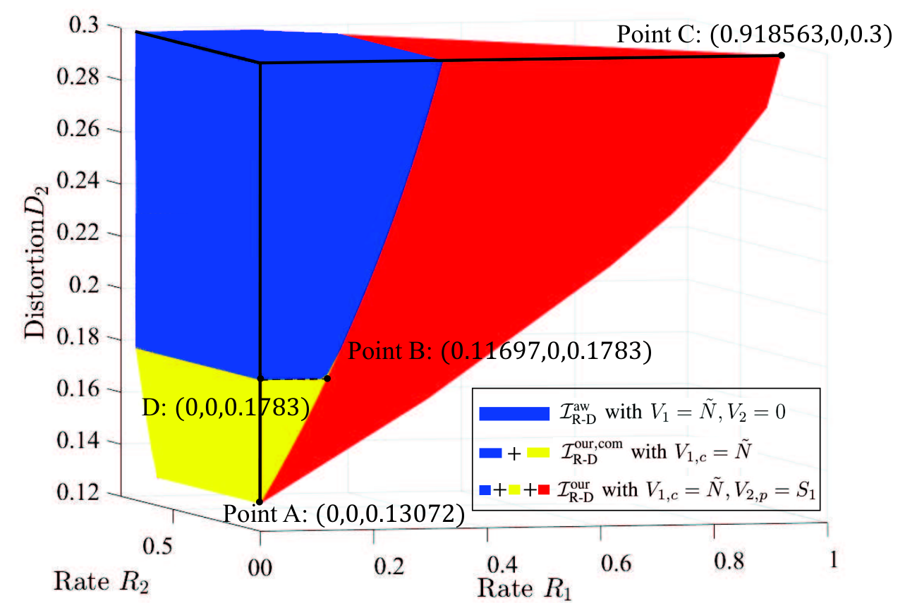
In this example, transmitter 1 can always achieve zero distortion, and we thus focus on the achievable region (R1,R2,D2)(R_{1},R_{2},D_{2}). Note that even for the considered binary example, the explictly characterizations of both our results ℐR-Dour,ℐR-Dour,com\mathcal{I}_{\text{R-D}}^{\text{our}},\mathcal{I}_{\text{R-D}}^{\text{our},\text{com}} and the existing one ℐR-Daw\mathcal{I}_{\text{R-D}}^{\text{aw}} of [17, Theorem 3] are intractable due to the presence of auxiliary random variables with large alphabet sizes that hinders an exhaustive search. To cope with this challenge, we first evaluate ℐR-Daw,ℐR-Dour,com,ℐR-Dour\mathcal{I}_{\text{R-D}}^{\text{aw}},\mathcal{I}_{\text{R-D}}^{\text{our},\text{com}},\mathcal{I}_{\text{R-D}}^{\text{our}} by considering some particular choice of random variables involved in the rate-distortion characterization. Then, we theoretically prove that ℐR-Daw⊊ℐR-Dour,com⊊ℐR-Dour\mathcal{I}_{\text{R-D}}^{\text{aw}}\subsetneq\mathcal{I}_{\text{R-D}}^{\text{our},\text{com}}\subsetneq\mathcal{I}_{\text{R-D}}^{\text{our}}, i.e., our results strictly include the existing one, regardless of the choice of the random variables.
Refer to caption
Fig. 6: An illustration of (R1,R2,D2)(R_{1},R_{2},D_{2}) tradeoff for Example 4 with the considered coding scheme.

We consider the following choice of random variables to evaluate region ℐR-Dour\mathcal{I}_{\text{R-D}}^{\text{our}}:

Xk=Uk⊕Θk=U⊕Σk⊕Θk,k∈{1,2},\displaystyle X_{k}=U_{k}\oplus\Theta_{k}=U\oplus\Sigma_{k}\oplus\Theta_{k},\ k\in\{1,2\}, (36a)
V1,c=N~,V2,p=S1,\displaystyle V_{1,c}=\tilde{N},\ V_{2,p}=S_{1}, (36b)
V1,p=v1,p∗,V2,c=v2,c∗,\displaystyle V_{1,p}=v^{*}_{1,p},\ V_{2,c}=v^{*}_{2,c}, (36c)

where U,Σ1,Σ2,Θ1,Θ2U,\Sigma_{1},\Sigma_{2},\Theta_{1},\Theta_{2} are independent binary random variables, N=N~⊕EN=\tilde{N}\oplus E, and E∼Bern​(PE)E\sim\text{Bern}(P_{E}) is a binary quantization variable with PE​(1)∈[0,PN​(1)]P_{E}(1)\in[0,P_{N}(1)], and V1,p=v1,p∗,V2,c=v2,c∗V_{1,p}=v^{*}_{1,p},V_{2,c}=v^{*}_{2,c} almost surely for some specific values v1,p∗∈𝒱1,p,v2,c∗∈𝒱2,cv^{*}_{1,p}\in\mathcal{V}_{1,p},v^{*}_{2,c}\in\mathcal{V}_{2,c}. For ℐR-Dour,com\mathcal{I}_{\text{R-D}}^{\text{our},\text{com}}, we still consider (36a), (36b), and (36c) except that V2,p=v2,p∗V_{2,p}=v^{*}_{2,p} almost surely for some specific value v2,p∗∈𝒱2,pv^{*}_{2,p}\in\mathcal{V}_{2,p}. To characterize region ℐR-Daw\mathcal{I}_{\text{R-D}}^{\text{aw}}, we consider (36a) and set variables V1=N~V_{1}=\tilde{N} and V2=v2∗V_{2}=v^{*}_{2} almost surely for some specific value v2∗∈𝒱2v^{*}_{2}\in\mathcal{V}_{2} . For the above choices of random variables, the achievable regions of all three schemes are presented in Fig. 6.

It can be shown that tuples (R1,R2,D2)=(0,0,0.13072)(R_{1},R_{2},D_{2})=(0,0,0.13072) and (0.11697,0,0.1783)(0.11697,0,0.1783) are in ℐR-Dour,com\mathcal{I}_{\text{R-D}}^{\text{our},\text{com}} (as shown in Fig. 6) but not in ℐR-Daw\mathcal{I}_{\text{R-D}}^{\text{aw}}, and tuple (0.918563,0,0.3)(0.918563,0,0.3) is in ℐR-Dour\mathcal{I}_{\text{R-D}}^{\text{our}} (as shown in Fig. 6) but not in ℐR-Dour,com\mathcal{I}_{\text{R-D}}^{\text{our},\text{com}}. Together with Theorem 2, we have

ℐR-Daw⊊ℐR-Dour,com⊊ℐR-Dour\displaystyle\mathcal{I}_{\text{R-D}}^{\text{aw}}\subsetneq\mathcal{I}_{\text{R-D}}^{\text{our},\text{com}}\subsetneq\mathcal{I}_{\text{R-D}}^{\text{our}} (37)

for this channel.

Proof:

The proof of ℐR-Daw⊊ℐR-Dour,com⊊ℐR-Dour\mathcal{I}_{\text{R-D}}^{\text{aw}}\subsetneq\mathcal{I}_{\text{R-D}}^{\text{our},\text{com}}\subsetneq\mathcal{I}_{\text{R-D}}^{\text{our}} can be found in Appendix F. ∎

IV-C2 Characterization of outer bounds

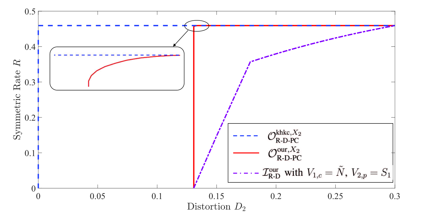
Transmitter 1 can always achieve zero distortion, and we notice that both 𝒪R-Dour\mathcal{O}_{\text{R-D}}^{\text{our}} and 𝒪R-Dkhkc\mathcal{O}_{\text{R-D}}^{\text{khkc}} are based on the idea of dependence balance and have the same results on communication when ignoring the sensing task. Therefore, we focus on the tradeoff between symmetric rate R1=R2=RR_{1}=R_{2}=R and distrotion D2D_{2}.

It should be noted that the evaluations of outer bounds 𝒪R-Dour\mathcal{O}_{\text{R-D}}^{\text{our}} and 𝒪R-Dkhkc\mathcal{O}_{\text{R-D}}^{\text{khkc}} are intractable due to the fact that the large cardinality of involved auxiliary random variables prohibits an exhaustive search [20]. To address these challenges, we apply the technique of [20] by introducing an adaptive parallel channel extension for the dependence balance bound and using a composite function ϕ⁡(t)=1−|1−2​t|2,t∈[0,1]\phi(t)=\frac{1-\sqrt{|1-2t|}}{2},\ t\in[0,1] and its properties to evaluate both our outer bound 𝒪R-Dour\mathcal{O}_{\text{R-D}}^{\text{our}} and the existing one 𝒪R-Dkhkc\mathcal{O}_{\text{R-D}}^{\text{khkc}}, denoted as 𝒪R-D-PCour,X2\mathcal{O}_{\text{R-D-PC}}^{\text{our},X_{2}} and 𝒪R-D-PCkhkc,X2\mathcal{O}_{\text{R-D-PC}}^{\text{khkc},X_{2}}, respectively. The details are given in Appendix G.
Refer to caption
Fig. 7: An illustration of the symmetric–rate-distortion tradeoff (R1=R2=R,D2)(R_{1}=R_{2}=R,D_{2}) for Example 4.

Based on the parallel channel extension, one can conduct numerical characterization of symmetric–rate-distortion region (R1=R2=R,D2)(R_{1}=R_{2}=R,D_{2}) for 𝒪R-D-PCour,X2\mathcal{O}_{\text{R-D-PC}}^{\text{our},X_{2}}, which is an outer bound of 𝒪R-Dour\mathcal{O}_{\text{R-D}}^{\text{our}} in Theorem 3. The same technique can be applied to get a valid outer bound 𝒪R-D-PCkhkc,X2\mathcal{O}_{\text{R-D-PC}}^{\text{khkc},X_{2}} for the results 𝒪R-Dkhkc\mathcal{O}_{\text{R-D}}^{\text{khkc}} in [14] and to characterize the symmetric–rate-distortion region (R1=R2=R,D2)(R_{1}=R_{2}=R,D_{2}) in 𝒪R-D-PCkhkc,X2\mathcal{O}_{\text{R-D-PC}}^{\text{khkc},X_{2}}. We note that outer bounds 𝒪R-Dour\mathcal{O}_{\text{R-D}}^{\text{our}} and 𝒪R-Dkhkc\mathcal{O}_{\text{R-D}}^{\text{khkc}} both use the idea of dependence balance. Thus, such a parallel channel extension results in the same performance on communication. Moreover, since the genie-aided state estimators are considered in 𝒪R-Dkhkc\mathcal{O}_{\text{R-D}}^{\text{khkc}}, the parallel channel extension ZPC=X2Z_{\text{PC}}=X_{2} does not effect sensing performance for 𝒪R-Dkhkc\mathcal{O}_{\text{R-D}}^{\text{khkc}}. Therefore, such a characterization can demonstrate the advantages of our improved outer bound on sensing performance.

The results are shown in Fig. 7, which shows that our outer bound is tighter than state-of-the-art [14]. Specifically, one can easily check that tuple (R=0,D2=0)(R=0,D_{2}=0) is in 𝒪R-Dkhkc\mathcal{O}_{\text{R-D}}^{\text{khkc}} but not in 𝒪R-Dour\mathcal{O}_{\text{R-D}}^{\text{our}}, which reveals that

𝒪R-Dour⊊𝒪R-Dkhkc.\displaystyle\mathcal{O}_{\text{R-D}}^{\text{our}}\subsetneq\mathcal{O}_{\text{R-D}}^{\text{khkc}}. (38)

Moreover, it can also be seen that our proposed scheme can achieve the sensing-optimal point (D2,min,0)(D_{2,\text{min}},0) and communication-optimal point (D2,max,Rmax)(D_{2,\text{max}},R_{\text{max}}), while for certain distortion constraint such as D2=0.2D_{2}=0.2, how to achieve the optimal performance for ISAC still remains open.

Remark 10.

The results and analysis presented in Example 4 demonstrate the following facts:

  1. 1.

    For the inner bound, the performance gain of our proposed scheme is two-fold. First, by allowing transmitters to cooperatively retransmit the common compressed information (V1,c,V2,c)(V_{1,c},V_{2,c}) in a similar manner to messsage coopeartion, our achievable scheme can get a better sensing performance (point A in Fig. 6), and enlarge the rate-region (point B) for the same distortion (point D (0,0,0.1783)(0,0,0.1783) is in ℐR-Daw\mathcal{I}_{\text{R-D}}^{\text{aw}}) that the existing one can achieve. The reason behind this improvement is that compressed information cooperation between two transmitters leverages the beamforming gain, which results in transmitting a larger amount of common compressed information (V1,c,V2,c)(V_{1,c},V_{2,c}). Second, allowing the transmitter 2 to send private compressed information V2,p=S1V_{2,p}=S_{1} decoded by the receiver only conveys information about channel states, facilitating the message decoding of W1W_{1} at the receiver and enlarging the rate region (point C).

  2. 2.

    For the outer bound, our results introduce additional rate-limited constraints on sensing performance, which provides a tighter bound for sensing performance, and thus a tighter outer bound for capacity-distortion region.

V Conclusion

In this paper, we have investigated the fundamental limits of ISAC over SD-DM MACs with correlated sensing state parameters and channel states. A new achievable scheme that combines message cooperation and joint compression of past transmitted codewords and echo signals has been proposed, and the corresponding inner bound of the capacity-distortion region has been proved to include that of [17, Theorem 3]. We have also established an improved outer bound of the capacity-distortion region by introducing the rate-limited constraints on sensing. It has been demonstrated, through several numerical examples, that the improved inner bound can achieve better communication and sensing performance, and the proposed outer bound strictly improves the existing one. We finally remark that while the inner and outer bounds presented in this paper improve upon the existing results [14, 17], the optimal capacity-distortion region for the model considered remains open. Future work includes further tightening the bounds for ISAC over MACs and investigation of the fundamental limits of other multi-terminal ISAC building blocks, such as in broadcast and relay channels.

Appendix A Proof of Theorem 1

The achievable scheme proposed, which combines with implicit binning, block Markov encoding, and backward decoding, consists of B+B~B+\tilde{B} transmission blocks. The last B~\tilde{B} blocks called “termination blocks” are necessary to guarantee that the receiver can successfully obtain the compressed information corresponding to blocks BB and B−1B-1. We first focus on the first BB blocks by assuming that the receiver can successfully obtain compressed information corresponding to blocks BB and B−1B-1. Then, the detailed discussion of termination blocks is presented.

A-A The Proposed Coding Scheme

Each of the first BB blocks is of length NN channel uses. Transmitter kk transmits B−1B-1 i.i.d. messages {wk(b)}b=1B−1\{w_{k}^{(b)}\}_{b=1}^{B-1} over B+B~B+\tilde{B} blocks. Each message wk(b)w_{k}^{(b)} is partitioned into two messages {wk,p(b),wk,c(b)}\{w_{k,p}^{(b)},w_{k,c}^{(b)}\}. The subscripts “p” and “c” here stand for “private” and “common”, respectively. The messages wk,p(b)∈[1:2N​Rk,p]w_{k,p}^{(b)}\in[1:2^{NR_{k,p}}] and wk,c(b)∈[1:2N​Rk,c]w_{k,c}^{(b)}\in[1:2^{NR_{k,c}}] are uniformly distributed and mutually independent for all k∈{1,2}k\in\{1,2\}, b∈[1:B−1]b\in[1:B-1], where Rk=Rk,p+Rk,cR_{k}=R_{k,p}+R_{k,c}. Let X1,(b)NX_{1,(b)}^{N}, X2,(b)NX_{2,(b)}^{N}, S(b)NS_{(b)}^{N}, ST1,(b)NS_{T_{1},(b)}^{N}, ST2,(b)NS_{T_{2},(b)}^{N}, Y(b)NY_{(b)}^{N}, Z1,(b)NZ_{1,(b)}^{N}, Z2,(b)NZ_{2,(b)}^{N} denote the inputs, states, sensing state parameters, outputs, and feedbacks in block bb.

A-A1 Codebook Generation

Fix a joint distribution PU​PU1|U​PU2|U​PX1|U​U1​PX2|U​U2​PS​ST1​ST2​PY​Z1​Z2|X1​X2​SP_{U}P_{U_{1}|U}P_{U_{2}|U}P_{X_{1}|UU_{1}}P_{X_{2}|UU_{2}}P_{SS_{T_{1}}S_{T_{2}}}P_{YZ_{1}Z_{2}|X_{1}X_{2}S} PV1,c​V1,p|U​U1​U2​X1​Z1​PV2,c​V2,p|U​U1​U2​X2​Z2​PS^T1|X1​Z1​U2​V2,cP_{V_{1,c}V_{1,p}|UU_{1}U_{2}X_{1}Z_{1}}P_{V_{2,c}V_{2,p}|UU_{1}U_{2}X_{2}Z_{2}}P_{\hat{S}_{T_{1}}|X_{1}Z_{1}U_{2}V_{2,c}}
PS^T2|X2​Z2​U1​V1,cP_{\hat{S}_{T_{2}}|X_{2}Z_{2}U_{1}V_{1,c}} as in Theorem 1, where PS​ST1​ST2P_{SS_{T_{1}}S_{T_{2}}} PY​Z1​Z2|X1​X2​SP_{YZ_{1}Z_{2}|X_{1}X_{2}S} is defined by the channel. Let Rk=Rk,p+Rk,cR_{k}=R_{k,p}+R_{k,c}, Rk,c≥0,Rk,p≥0,Rvk,c≥0,Rvk,p≥0R_{k,c}\geq 0,R_{k,p}\geq 0,R_{v_{k,c}}\geq 0,R_{v_{k,p}}\geq 0, k∈{1,2}k\in\{1,2\}. For block b∈[1:B]b\in[1:B], an illustration of constructed codebook is presented in Fig. 8, and the detailed codebook is as follows.

Fig. 8: An illustration of codebook generation in block bb.
  • •

    Generate 2N⁡(R1,c+Rv1,c+R2,c+Rv2,c)2^{N(R_{1,c}+R_{v_{1,c}}+R_{2,c}+R_{v_{2,c}})} sequences u(b)N​(CLOSEu_{(b)}^{N}( OPENjb−1,lb−1,kb−1,mb−1)j_{b-1},l_{b-1},k_{b-1},m_{b-1}), jb−1∈[1:2N​R1,c]j_{b-1}\in[1:2^{NR_{1,c}}], lb−1∈l_{b-1}\in [1:2N​Rv1,c][1:2^{NR_{v_{1,c}}}], kb−1∈[1:2N​R2,c]k_{b-1}\in[1:2^{NR_{2,c}}], mb−1∈[1:2N​Rv2,c]m_{b-1}\in[1:2^{NR_{v_{2,c}}}], i.i.d. according to PU​(⋅)P_{U}(\cdot).

  • •

    For each tuple (jb−1,lb−1,kb−1,mb−1)(j_{b-1},l_{b-1},k_{b-1},m_{b-1}), generate 2N⁡(R1,c+Rv1,c)2^{N(R_{1,c}+R_{v_{1,c}})} sequences u1,(b)N​(jb−1,lb−1,kb−1,mb−1CLOSE,u_{1,(b)}^{N}(j_{b-1},l_{b-1},k_{b-1},m_{b-1}, OPENjb,lb)j_{b},l_{b}), jb∈[1:2N​R1,c]j_{b}\in[1:2^{NR_{1,c}}]. lb∈[1:l_{b}\in[1: 2N​Rv1,c]2^{NR_{v_{1,c}}}], i.i.d. according to PU1|U(⋅|u)P_{U_{1}|U}(\cdot|u). Similarly, generate 2N⁡(R2,c+Rv2,c)2^{N(R_{2,c}+R_{v_{2,c}})} sequences u2,(b)N​(jb−1,lb−1,kb−1,mb−1,kb,mb)u_{2,(b)}^{N}(j_{b-1},l_{b-1},k_{b-1},m_{b-1},k_{b},m_{b}) i.i.d. according to PU2|U(⋅|u)P_{U_{2}|U}(\cdot|u).

  • •

    For each tuple (jb−1,lb−1,kb−1,mb−1,jb,lb)(j_{b-1},l_{b-1},k_{b-1},m_{b-1},j_{b},l_{b}), generate 2N⁡(R1,p+Rv1,p)2^{N(R_{1,p}+R_{v_{1,p}})} sequences x1,(b)N​(jb−1,lb−1,kb−1CLOSE,x_{1,(b)}^{N}(j_{b-1},l_{b-1},k_{b-1}, OPENmb−1,jb,lb,rb,αb)m_{b-1},j_{b},l_{b},r_{b},\alpha_{b}), rb∈[1:2N​R1,p]r_{b}\in[1:2^{NR_{1,p}}], αb\alpha_{b} ∈[1:2N​Rv1,p]\in[1:2^{NR_{v_{1,p}}}] i.i.d. according to PX1|U​U1P_{X_{1}|UU_{1}} (⋅|uu1)(\cdot|uu_{1}). Similarly, generate 2N⁡(R2,p+Rv2,p)2^{N(R_{2,p}+R_{v_{2,p}})} sequences x2,(b)N​(jb−1,lb−1,kb−1CLOSEx_{2,(b)}^{N}(j_{b-1},l_{b-1},k_{b-1}, OPENmb−1,kb,mb,sb,βb)m_{b-1},k_{b},m_{b},s_{b},\beta_{b}) i.i.d. according to PX2|U​U2(⋅|uu2)P_{X_{2}|UU_{2}}(\cdot|uu_{2}).

  • •

    For each tuple (jb−1,lb−1,kb−1,mb−1,jb,lb,kb,mb)(j_{b-1},l_{b-1},k_{b-1},m_{b-1},j_{b},l_{b},k_{b},m_{b}), generate 2N​Rv1,c2^{NR_{v_{1,c}}} sequences v1,c,(b)N​(jb−1,lb−1,kb−1CLOSE,v^{N}_{1,c,(b)}(j_{b-1},l_{b-1},k_{b-1}, OPENmb−1,jb,lb,kb,mb,lb+1)m_{b-1},j_{b},l_{b},k_{b},m_{b},l_{b+1}), lb+1∈[1:2N​Rv1,c]l_{b+1}\in[1:2^{NR_{v_{1,c}}}] i.i.d. according to PV1,c|U​U1​U2(⋅|uu1u2)P_{V_{1,c}|UU_{1}U_{2}}(\cdot|uu_{1}u_{2}). Similarly, generate 2N​Rv2,c2^{NR_{v_{2,c}}} sequences v2,c,(b)N​(jb−1,lb−1,kb−1CLOSE,v^{N}_{2,c,(b)}(j_{b-1},l_{b-1},k_{b-1}, OPENmb−1,jb,lb,kb,mb,mb+1)m_{b-1},j_{b},l_{b},k_{b},m_{b},m_{b+1}), mb+1∈[1:2N​Rv2,c]m_{b+1}\in[1:2^{NR_{v_{2,c}}}] i.i.d. according to PV2,c|U​U1​U2(⋅|uu1u2)P_{V_{2,c}|UU_{1}U_{2}}(\cdot|uu_{1}u_{2}).

  • •

    For each tuple (jb−1,lb−1,kb−1,mb−1,jb,lb,kb,mb,rbCLOSE,(j_{b-1},l_{b-1},k_{b-1},m_{b-1},j_{b},l_{b},k_{b},m_{b},r_{b}, OPENαb,lb+1)\alpha_{b},l_{b+1}), generate 2N​Rv1,p2^{NR_{v_{1,p}}} sequences v1,p,(b)N​(jb−1CLOSE,v^{N}_{1,p,(b)}(j_{b-1}, OPENlb−1,kb−1,mb−1,jb,lb,kb,mb,rb,αb,lb+1,αb+1)l_{b-1},k_{b-1},m_{b-1},j_{b},l_{b},k_{b},m_{b},r_{b},\alpha_{b},l_{b+1},\alpha_{b+1}), αb+1∈\alpha_{b+1}\in [1:2N​Rv1,p][1:2^{NR_{v_{1,p}}}] i.i.d. according to PV1,p|U​U1​U2​X1​V1,c(⋅|uu1u2x1v1,c)P_{V_{1,p}|UU_{1}U_{2}X_{1}V_{1,c}}(\cdot|uu_{1}u_{2}x_{1}v_{1,c}), Similarly, generate 2N​Rv2,p2^{NR_{v_{2,p}}} sequences v2,p,(b)N​(CLOSEv^{N}_{2,p,(b)}( jb−1,lb−1,kb−1,mb−1,jb,lb,j_{b-1},l_{b-1},k_{b-1},m_{b-1},j_{b},l_{b}, OPENkb,mb,sb,βb,mb+1,βb+1)k_{b},m_{b},s_{b},\beta_{b},m_{b+1},\beta_{b+1}), βb+1∈[1:2N​Rv2,p]\beta_{b+1}\in[1:2^{NR_{v_{2,p}}}] i.i.d. according to PV2,p|U​U1​U2​X2​V2,c(⋅|uu1u2x2v2,c)P_{V_{2,p}|UU_{1}U_{2}X_{2}V_{2,c}}(\cdot|uu_{1}u_{2}x_{2}v_{2,c}).

A-A2 Encoding

We set j0=k0=1j_{0}=k_{0}=1, l0=m0=1l_{0}=m_{0}=1, l1=m1=1l_{1}=m_{1}=1, α1=β1=1\alpha_{1}=\beta_{1}=1, jB=kB=rB=sB=1j_{B}=k_{B}=r_{B}=s_{B}=1. The detailed encoding is as follows, and a brief illustration is provided in Fig. 9.

Fig. 9: Encoding operations in the first BB blocks.
  • •

    Block b=1b=1. Two transmitters send x1,(1)N​(1,1,1,1,j1,1CLOSE,x_{1,(1)}^{N}(1,1,1,1,j_{1},1, OPENr1,1)r_{1},1) and x2,(1)N​(1,1,1,1,k1,1,s1,1)x_{2,(1)}^{N}(1,1,1,1,k_{1},1,s_{1},1), respectively.

  • •

    Block b∈[2:B+1]b\in[2:B+1]. At the beginning of block bb, where b∈[2:B+1]b\in[2:B+1], transmitter 1 obtains generalized feedback z1,(b−1)Nz^{N}_{1,(b-1)} and indices tuple (jb−2∗,lb−2∗,kb−2∗,mb−2∗,jb−1∗,lb−1∗,rb−1∗,αb−1∗)(j^{*}_{b-2},l^{*}_{b-2},k^{*}_{b-2},m^{*}_{b-2},j^{*}_{b-1},l^{*}_{b-1},r^{*}_{b-1},\alpha^{*}_{b-1}). If b∈[3:B]b\in[3:B], it also knows indices tuple (jb−3∗,lb−3∗,kb−3∗,mb−3∗,rb−2∗,αb−2∗)(j^{*}_{b-3},l^{*}_{b-3},k^{*}_{b-3},m^{*}_{b-3},r^{*}_{b-2},\alpha^{*}_{b-2}) and generalized feedback z1,(b−2)Nz^{N}_{1,(b-2)}. Thus, at the beginning of block bb, transmitter 1 finds a unique pair (k^b−1,m^b−1)∈[1:2N​R2,c]×[1:2N​Rv2,c](\hat{k}_{b-1},\hat{m}_{b-1})\in[1:2^{NR_{2,c}}]\times[1:2^{NR_{v_{2,c}}}] satisfying

    (\displaystyle\bigg( u(b−1)N​(jb−2∗,lb−2∗,kb−2∗,mb−2∗),\displaystyle u^{N}_{(b-1)}(j^{*}_{b-2},l^{*}_{b-2},k^{*}_{b-2},m^{*}_{b-2}),
    u1,(b−1)N​(jb−2∗,lb−2∗,kb−2∗,mb−2∗,jb−1∗,lb−1∗),\displaystyle u^{N}_{1,(b-1)}(j^{*}_{b-2},l^{*}_{b-2},k^{*}_{b-2},m^{*}_{b-2},j^{*}_{b-1},l^{*}_{b-1}),
    u2,(b−1)N​(jb−2∗,lb−2∗,kb−2∗,mb−2∗,k^b−1,m^b−1),\displaystyle u^{N}_{2,(b-1)}(j^{*}_{b-2},l^{*}_{b-2},k^{*}_{b-2},m^{*}_{b-2},\hat{k}_{b-1},\hat{m}_{b-1}),
    x1,(b−1)N​(jb−2∗,lb−2∗,kb−2∗,mb−2∗,jb−1∗,lb−1∗,rb−1∗,αb−1∗),\displaystyle x^{N}_{1,(b-1)}(j^{*}_{b-2},l^{*}_{b-2},k^{*}_{b-2},m^{*}_{b-2},j^{*}_{b-1},l^{*}_{b-1},r^{*}_{b-1},\alpha^{*}_{b-1}),
    OPENz1,(b−1)N)∈𝒯ϵN​(U​U1​U2​X1​Z1),\displaystyle z^{N}_{1,(b-1)}\bigg)\in\mathcal{T}_{\epsilon}^{N}(UU_{1}U_{2}X_{1}Z_{1}), (39)

    and

    (\displaystyle\bigg( u(b−2)N​(jb−3∗,lb−3∗,kb−3∗,mb−3∗),\displaystyle u^{N}_{(b-2)}(j^{*}_{b-3},l^{*}_{b-3},k^{*}_{b-3},m^{*}_{b-3}),
    u1,(b−2)N​(jb−3∗,lb−3∗,kb−3∗,mb−3∗,jb−2∗,lb−2∗),\displaystyle u^{N}_{1,(b-2)}(j^{*}_{b-3},l^{*}_{b-3},k^{*}_{b-3},m^{*}_{b-3},j^{*}_{b-2},l^{*}_{b-2}),
    u2,(b−2)N​(jb−3∗,lb−3∗,kb−3∗,mb−3∗,kb−2∗,mb−2∗),\displaystyle u^{N}_{2,(b-2)}(j^{*}_{b-3},l^{*}_{b-3},k^{*}_{b-3},m^{*}_{b-3},k^{*}_{b-2},m^{*}_{b-2}),
    x1,(b−2)N​(jb−3∗,lb−3∗,kb−3∗,mb−3∗,jb−2∗,lb−2∗,rb−2∗,αb−2∗),\displaystyle x^{N}_{1,(b-2)}(j^{*}_{b-3},l^{*}_{b-3},k^{*}_{b-3},m^{*}_{b-3},j^{*}_{b-2},l^{*}_{b-2},r^{*}_{b-2},\alpha^{*}_{b-2}),
    v2,c,(b−2)N​(jb−3∗,lb−3∗,kb−3∗,mb−3∗,jb−2∗,lb−2∗,kb−2∗,mb−2∗CLOSE,\displaystyle v^{N}_{2,c,(b-2)}(j^{*}_{b-3},l^{*}_{b-3},k^{*}_{b-3},m^{*}_{b-3},j^{*}_{b-2},l^{*}_{b-2},k^{*}_{b-2},m^{*}_{b-2},
    OPENOPENm^b−1),z1,(b−2)N)∈𝒯ϵN​(U​U1​U2​X1​V2,c​Z1)\displaystyle\hat{m}_{b-1}),z^{N}_{1,(b-2)}\bigg)\in\mathcal{T}_{\epsilon}^{N}(UU_{1}U_{2}X_{1}V_{2,c}Z_{1}) (40)

    simultaneously. For b=2b=2, only (• ‣ A-A2) needs to be satisfied. If there is exactly one pair (k^b−1,m^b−1)(\hat{k}_{b-1},\hat{m}_{b-1}) satisfying the above conditions, transmitter 1 sets kb−1∗=k^b−1k^{*}_{b-1}=\hat{k}_{b-1}, mb−1∗=m^b−1m^{*}_{b-1}=\hat{m}_{b-1}. Otherwise, an error is declared. Once obtaining the correct indices pair (kb−1∗CLOSE(k^{*}_{b-1}, OPENmb−1∗)m^{*}_{b-1}), transmitter 1 finds a pair (l^b,α^b)∈[1:2N​Rv1,c]×[1:2N​Rv1,p](\hat{l}_{b},\hat{\alpha}_{b})\in[1:2^{NR_{v_{1,c}}}]\times[1:2^{NR_{v_{1,p}}}] satisfying

    (\displaystyle\bigg( u(b−1)N​(jb−2∗,lb−2∗,kb−2∗,mb−2∗),\displaystyle u^{N}_{(b-1)}(j^{*}_{b-2},l^{*}_{b-2},k^{*}_{b-2},m^{*}_{b-2}),
    u1,(b−1)N​(jb−2∗,lb−2∗,kb−2∗,mb−2∗,jb−1∗,lb−1∗),\displaystyle u^{N}_{1,(b-1)}(j^{*}_{b-2},l^{*}_{b-2},k^{*}_{b-2},m^{*}_{b-2},j^{*}_{b-1},l^{*}_{b-1}),
    u2,(b−1)N​(jb−2∗,lb−2∗,kb−2∗,mb−2∗,kb−1∗,mb−1∗),\displaystyle u^{N}_{2,(b-1)}(j^{*}_{b-2},l^{*}_{b-2},k^{*}_{b-2},m^{*}_{b-2},k^{*}_{b-1},m^{*}_{b-1}),
    x1,(b−1)N​(jb−2∗,lb−2∗,kb−2∗,mb−2∗,jb−1∗,lb−1∗,rb−1∗,αb−1∗),\displaystyle x^{N}_{1,(b-1)}(j^{*}_{b-2},l^{*}_{b-2},k^{*}_{b-2},m^{*}_{b-2},j^{*}_{b-1},l^{*}_{b-1},r^{*}_{b-1},\alpha^{*}_{b-1}),
    v1,c,(b−1)N​(jb−2∗,lb−2∗,kb−2∗,mb−2∗,jb−1∗,lb−1∗,kb−1∗CLOSE,\displaystyle v^{N}_{1,c,(b-1)}(j^{*}_{b-2},l^{*}_{b-2},k^{*}_{b-2},m^{*}_{b-2},j^{*}_{b-1},l^{*}_{b-1},k^{*}_{b-1},
    OPENmb−1∗,l^b),v1,p,(b−1)N​(jb−2∗,lb−2∗,kb−2∗,mb−2∗,jb−1∗,lb−1∗CLOSE,\displaystyle m^{*}_{b-1},\hat{l}_{b}),v^{N}_{1,p,(b-1)}(j^{*}_{b-2},l^{*}_{b-2},k^{*}_{b-2},m^{*}_{b-2},j^{*}_{b-1},l^{*}_{b-1},
    OPENOPENkb−1∗,mb−1∗,rb−1∗,αb−1∗,l^b,α^b),z1,(b−1)N)\displaystyle k^{*}_{b-1},m^{*}_{b-1},r^{*}_{b-1},\alpha^{*}_{b-1},\hat{l}_{b},\hat{\alpha}_{b}),z^{N}_{1,(b-1)}\bigg)
    ∈𝒯ϵN​(U​U1​U2​X1​V1,c​V1,p​Z1).\displaystyle\in\mathcal{T}_{\epsilon}^{N}(UU_{1}U_{2}X_{1}V_{1,c}V_{1,p}Z_{1}). (41)

    and sets lb∗=l^b,αb∗=α^bl^{*}_{b}=\hat{l}_{b},\alpha^{*}_{b}=\hat{\alpha}_{b}. If there is no such pair, transmitter 1 sets lb∗=1,αb∗=1l^{*}_{b}=1,\alpha^{*}_{b}=1. Then, transmitter 1 sends x1,(b)N​(jb−1∗,lb−1∗,kb−1∗,mb−1∗,jb,lb∗,rb,αb∗)x^{N}_{1,(b)}(j^{*}_{b-1},l^{*}_{b-1},k^{*}_{b-1},m^{*}_{b-1},j_{b},l^{*}_{b},r_{b},\alpha^{*}_{b}) in block b∈[2:B]b\in[2:B]. The operations at transmitter 2 are analogous and omitted here.

A-A3 Decoding

Fig. 10: Decoding operations in the first BB blocks.

Decoding begins at the block BB and proceeds backward. A brief illustration of decoding operations is provided in Fig. 10, and the details are as follows. In block b∈[B:1]b\in[B:1], the receiver has observed channel output y(b)Ny^{N}_{(b)}. It also has the correct indices tuple (jb∗,lb∗,kb∗,mb∗)(j^{*}_{b},l^{*}_{b},k^{*}_{b},m^{*}_{b}) and (lb+1∗,mb+1∗,αb+1∗,βb+1∗)(l^{*}_{b+1},m^{*}_{b+1},\alpha^{*}_{b+1},\beta^{*}_{b+1}) by the decoding procedures in block b+1b+111 1 For block b=Bb=B, this is guaranteed by termination blocks.. The receiver finds a unique tuple (j^b−1,l^b−1,k^b−1,m^b−1,r^b,α^b,s^b,β^b)∈[1:2N​R1,c]×[1:2N​Rv1,c]×[1:2N​R2,c]×[1:2N​Rv2,c]×[1:2N​R1,p]×[1:2N​Rv1,p]×[1:2N​R2,p]×[1:2N​Rv2,p](\hat{j}_{b-1},\hat{l}_{b-1},\hat{k}_{b-1},\hat{m}_{b-1},\hat{r}_{b},\hat{\alpha}_{b},\hat{s}_{b},\hat{\beta}_{b})\in[1:2^{NR_{1,c}}]\times[1:2^{NR_{v_{1,c}}}]\times[1:2^{NR_{2,c}}]\times[1:2^{NR_{v_{2,c}}}]\times[1:2^{NR_{1,p}}]\times[1:2^{NR_{v_{1,p}}}]\times[1:2^{NR_{2,p}}]\times[1:2^{NR_{v_{2,p}}}] such that

(\displaystyle\bigg( u(b)N​(j^b−1,l^b−1,k^b−1,m^b−1),\displaystyle u^{N}_{(b)}(\hat{j}_{b-1},\hat{l}_{b-1},\hat{k}_{b-1},\hat{m}_{b-1}),
u1,(b)N​(j^b−1,l^b−1,k^b−1,m^b−1,jb∗,lb∗),\displaystyle u^{N}_{1,(b)}(\hat{j}_{b-1},\hat{l}_{b-1},\hat{k}_{b-1},\hat{m}_{b-1},j^{*}_{b},l^{*}_{b}),
u2,(b)N​(j^b−1,l^b−1,k^b−1,m^b−1,kb∗,mb∗),\displaystyle u^{N}_{2,(b)}(\hat{j}_{b-1},\hat{l}_{b-1},\hat{k}_{b-1},\hat{m}_{b-1},k^{*}_{b},m^{*}_{b}),
x1,(b)N​(j^b−1,l^b−1,k^b−1,m^b−1,jb∗,lb∗,r^b,α^b),\displaystyle x^{N}_{1,(b)}(\hat{j}_{b-1},\hat{l}_{b-1},\hat{k}_{b-1},\hat{m}_{b-1},j^{*}_{b},l^{*}_{b},\hat{r}_{b},\hat{\alpha}_{b}),
x2,(b)N​(j^b−1,l^b−1,k^b−1,m^b−1,kb∗,mb∗,s^b,β^b),\displaystyle x^{N}_{2,(b)}(\hat{j}_{b-1},\hat{l}_{b-1},\hat{k}_{b-1},\hat{m}_{b-1},k^{*}_{b},m^{*}_{b},\hat{s}_{b},\hat{\beta}_{b}),
v1,c,(b)N​(j^b−1,l^b−1,k^b−1,m^b−1,jb∗,lb∗,kb∗,mb∗,lb+1∗),\displaystyle v^{N}_{1,c,(b)}(\hat{j}_{b-1},\hat{l}_{b-1},\hat{k}_{b-1},\hat{m}_{b-1},j^{*}_{b},l^{*}_{b},k^{*}_{b},m^{*}_{b},l^{*}_{b+1}),
v2,c,(b)N​(j^b−1,l^b−1,k^b−1,m^b−1,jb∗,lb∗,kb∗,mb∗,mb+1∗)\displaystyle v^{N}_{2,c,(b)}(\hat{j}_{b-1},\hat{l}_{b-1},\hat{k}_{b-1},\hat{m}_{b-1},j^{*}_{b},l^{*}_{b},k^{*}_{b},m^{*}_{b},m^{*}_{b+1})
v1,p,(b)N​(j^b−1,l^b−1,k^b−1,m^b−1,jb∗,lb∗,kb∗,mb∗,r^b,α^b,lb+1∗CLOSE,\displaystyle v^{N}_{1,p,(b)}(\hat{j}_{b-1},\hat{l}_{b-1},\hat{k}_{b-1},\hat{m}_{b-1},j^{*}_{b},l^{*}_{b},k^{*}_{b},m^{*}_{b},\hat{r}_{b},\hat{\alpha}_{b},l^{*}_{b+1},
OPENαb+1∗),v2,p,(b)N​(j^b−1,l^b−1,k^b−1,m^b−1,jb∗,lb∗,kb∗,mb∗,s^b,β^bCLOSE,\displaystyle\alpha^{*}_{b+1}),v^{N}_{2,p,(b)}(\hat{j}_{b-1},\hat{l}_{b-1},\hat{k}_{b-1},\hat{m}_{b-1},j^{*}_{b},l^{*}_{b},k^{*}_{b},m^{*}_{b},\hat{s}_{b},\hat{\beta}_{b},
OPENOPENmb+1∗,βb+1∗),y(b)N)\displaystyle m^{*}_{b+1},\beta^{*}_{b+1}),y^{N}_{(b)}\bigg)
∈𝒯ϵN​(U​U1​U2​X1​X2​V1,c​V2,c​V1,p​V2,p​Y).\displaystyle\in\mathcal{T}_{\epsilon}^{N}(UU_{1}U_{2}X_{1}X_{2}V_{1,c}V_{2,c}V_{1,p}V_{2,p}Y). (42)

If there is exactly one tuple (j^b−1,l^b−1,k^b−1,m^b−1CLOSE,(\hat{j}_{b-1},\hat{l}_{b-1},\hat{k}_{b-1},\hat{m}_{b-1}, OPENr^b,α^b,s^b,β^b)\hat{r}_{b},\hat{\alpha}_{b},\hat{s}_{b},\hat{\beta}_{b}) satisfying (A-A3), the receiver sets jb−1∗=j^b−1,lb−1∗=l^b−1,kb−1∗=k^b−1,mb−1∗=m^b−1,rb∗=r^b,αb∗=α^b,sb∗=s^b,βb∗=β^bj^{*}_{b-1}=\hat{j}_{b-1},l^{*}_{b-1}=\hat{l}_{b-1},k^{*}_{b-1}=\hat{k}_{b-1},m^{*}_{b-1}=\hat{m}_{b-1},r^{*}_{b}=\hat{r}_{b},\alpha^{*}_{b}=\hat{\alpha}_{b},s^{*}_{b}=\hat{s}_{b},\beta^{*}_{b}=\hat{\beta}_{b}. Otherwise, an error is declared. The message output of receiver is (jb∗,rb∗,kb∗,sb∗),b∈[1:B−1](j^{*}_{b},r^{*}_{b},k^{*}_{b},s^{*}_{b}),b\in[1:B-1].

A-A4 State Estimation

For block b∈[1:B−1]b\in[1:B-1], transmitter 1 has observed the generalized feedback z1,(b)Nz^{N}_{1,(b)}. By decoding operations corresponding to (• ‣ A-A2) and (• ‣ A-A2) at the end of block bb, it obtains correct indices pair (kb∗,mb∗)(k^{*}_{b},m^{*}_{b}) and thus knows the codeword u2,(b)N​(jb−1∗,lb−1∗,kb−1∗,mb−1∗,kb∗,mb∗)u^{N}_{2,(b)}(j^{*}_{b-1},l^{*}_{b-1},k^{*}_{b-1},m^{*}_{b-1},k^{*}_{b},m^{*}_{b}). Transmitter 1 can also obtain correct index mb+1∗m^{*}_{b+1} by the decoding procedures (• ‣ A-A2) and (• ‣ A-A2) performed at the end of block b+1b+1 and thus knows the codeword v2,c,(b)N​(jb−1∗,lb−1∗,kb−1∗,mb−1∗,jb∗,lb∗,kb∗CLOSE,v^{N}_{2,c,(b)}(j^{*}_{b-1},l^{*}_{b-1},k^{*}_{b-1},m^{*}_{b-1},j^{*}_{b},l^{*}_{b},k^{*}_{b}, OPENmb∗,mb+1∗)m^{*}_{b},m^{*}_{b+1}). Combined with its own transmitted codeword x1,(b)N​(jb−1∗,lb−1∗,kb−1∗,mb−1∗,jb∗,lb∗,rb∗,αb∗)x^{N}_{1,(b)}(j^{*}_{b-1},l^{*}_{b-1},k^{*}_{b-1},m^{*}_{b-1},j^{*}_{b},l^{*}_{b},r^{*}_{b},\alpha^{*}_{b}), it produces the estimated parameter sequence

s^T1,(b)N=s^T1​(CLOSE\displaystyle\hat{s}_{T_{1},(b)}^{N}=\hat{s}_{T_{1}}\bigg( x1,(b)N​(jb−1∗,lb−1∗,kb−1∗,mb−1∗,jb∗,lb∗,rb∗,αb∗),\displaystyle x^{N}_{1,(b)}(j^{*}_{b-1},l^{*}_{b-1},k^{*}_{b-1},m^{*}_{b-1},j^{*}_{b},l^{*}_{b},r^{*}_{b},\alpha^{*}_{b}),
u2,(b)N​(jb−1∗,lb−1∗,kb−1∗,mb−1∗,kb∗,mb∗),\displaystyle u^{N}_{2,(b)}(j^{*}_{b-1},l^{*}_{b-1},k^{*}_{b-1},m^{*}_{b-1},k^{*}_{b},m^{*}_{b}),
z1,(b)N,v2,c,(b)N​(jb−1∗,lb−1∗,kb−1∗,mb−1∗,jb∗,lb∗,kb∗CLOSE,\displaystyle z^{N}_{1,(b)},v^{N}_{2,c,(b)}(j^{*}_{b-1},l^{*}_{b-1},k^{*}_{b-1},m^{*}_{b-1},j^{*}_{b},l^{*}_{b},k^{*}_{b},
OPENOPENmb∗,mb+1∗))\displaystyle m^{*}_{b},m^{*}_{b+1})\bigg) (43)

by applying the symbol-by-symbol estimator defined in (1) for block b∈[1:B−1]b\in[1:B-1]. The operations at transmitter 2 are analogous and omitted here.

A-B Error Analysis

We focus on the error analysis of the first BB blocks. Denote by ℰTx,k\mathcal{E}_{\text{Tx},k} and ℰRx\mathcal{E}_{\text{Rx}} the “encoding error” event of transmitter k∈{1,2}k\in\{1,2\} and “decoding error” event of the receiver, respectively. By the union bound, we have

Pℰ≤P⁡(ℰTx,1)+P⁡(ℰTx,2)+P⁡(ℰRx).\displaystyle P_{\mathcal{E}}\leq P(\mathcal{E}_{\text{Tx},1})+P(\mathcal{E}_{\text{Tx},2})+P(\mathcal{E}_{\text{Rx}}). (44)

We proceed to derive an upper bound for each term in the right hand side of (44).

Error Analysis at the transmitter 1: The error probability of transmitter 1 can be bounded as

P⁡(ℰTx,1)≤P⁡(ℰTx,1,(2))+∑b=3BP⁡(ℰTx,1,(b))+P⁡(ℰTx,1,(B+1)),\displaystyle P(\mathcal{E}_{\text{Tx},1})\leq P(\mathcal{E}_{\text{Tx},1,(2)})+\sum_{b=3}^{B}P(\mathcal{E}_{\text{Tx},1,(b)})+P(\mathcal{E}_{\text{Tx},1,(B+1)}), (45)

where ℰTx,1,(b)\mathcal{E}_{\text{Tx},1,(b)} represents the error event of transmitter 11 in block bb.

We first bound P⁡(ℰTx,1,(b))P(\mathcal{E}_{\text{Tx},1,(b)}) for b∈[3:B]b\in[3:B]. Denote by 𝒜1,(b)\mathcal{A}_{1,(b)} the error events corresponding to (• ‣ A-A2) and (• ‣ A-A2), and by ℬ1,(b)\mathcal{B}_{1,(b)} the error event corresponding to (• ‣ A-A2). By the union bound, we have

P⁡(ℰTx,1,(b))≤P⁡(𝒜1,(b))+P⁡(ℬ1,(b)).\displaystyle P(\mathcal{E}_{\text{Tx},1,(b)})\leq P(\mathcal{A}_{1,(b)})+P(\mathcal{B}_{1,(b)}). (46)

For term P⁡(𝒜1,(b))P(\mathcal{A}_{1,(b)}), define

𝒜\displaystyle\mathcal{A} (k^b−1,m^b−1)1,(b)={(u(b−1)N(jb−2∗,lb−2∗,kb−2∗,mb−2∗),{}_{1,(b)}(\hat{k}_{b-1},\hat{m}_{b-1})=\bigg\{\bigg(u^{N}_{(b-1)}(j^{*}_{b-2},l^{*}_{b-2},k^{*}_{b-2},m^{*}_{b-2}),
u1,(b−1)N​(jb−2∗,lb−2∗,kb−2∗,mb−2∗,jb−1∗,lb−1∗),\displaystyle u^{N}_{1,(b-1)}(j^{*}_{b-2},l^{*}_{b-2},k^{*}_{b-2},m^{*}_{b-2},j^{*}_{b-1},l^{*}_{b-1}),
u2,(b−1)N​(jb−2∗,lb−2∗,kb−2∗,mb−2∗,k^b−1,m^b−1),\displaystyle u^{N}_{2,(b-1)}(j^{*}_{b-2},l^{*}_{b-2},k^{*}_{b-2},m^{*}_{b-2},\hat{k}_{b-1},\hat{m}_{b-1}),
x1,(b−1)N​(jb−2∗,lb−2∗,kb−2∗,mb−2∗,jb−1∗,lb−1∗,rb−1∗,αb−1∗),\displaystyle x^{N}_{1,(b-1)}(j^{*}_{b-2},l^{*}_{b-2},k^{*}_{b-2},m^{*}_{b-2},j^{*}_{b-1},l^{*}_{b-1},r^{*}_{b-1},\alpha^{*}_{b-1}),
OPENz1,(b−1)N)∈𝒯ϵN​(U​U1​U2​X1​Z1),\displaystyle z^{N}_{1,(b-1)}\bigg)\in\mathcal{T}_{\epsilon}^{N}(UU_{1}U_{2}X_{1}Z_{1}),
and
(\displaystyle\bigg( u(b−2)N​(jb−3∗,lb−3∗,kb−3∗,mb−3∗),\displaystyle u^{N}_{(b-2)}(j^{*}_{b-3},l^{*}_{b-3},k^{*}_{b-3},m^{*}_{b-3}),
u1,(b−2)N​(jb−3∗,lb−3∗,kb−3∗,mb−3∗,jb−2∗,lb−2∗),\displaystyle u^{N}_{1,(b-2)}(j^{*}_{b-3},l^{*}_{b-3},k^{*}_{b-3},m^{*}_{b-3},j^{*}_{b-2},l^{*}_{b-2}),
u2,(b−2)N​(jb−3∗,lb−3∗,kb−3∗,mb−3∗,kb−2∗,mb−2∗),\displaystyle u^{N}_{2,(b-2)}(j^{*}_{b-3},l^{*}_{b-3},k^{*}_{b-3},m^{*}_{b-3},k^{*}_{b-2},m^{*}_{b-2}),
x1,(b−2)N​(jb−3∗,lb−3∗,kb−3∗,mb−3∗,jb−2∗,lb−2∗,rb−2∗,αb−2∗),\displaystyle x^{N}_{1,(b-2)}(j^{*}_{b-3},l^{*}_{b-3},k^{*}_{b-3},m^{*}_{b-3},j^{*}_{b-2},l^{*}_{b-2},r^{*}_{b-2},\alpha^{*}_{b-2}),
v2,c,(b−2)N​(jb−3∗,lb−3∗,kb−3∗,mb−3∗,jb−2∗,lb−2∗,kb−2∗,mb−2∗CLOSE,\displaystyle v^{N}_{2,c,(b-2)}(j^{*}_{b-3},l^{*}_{b-3},k^{*}_{b-3},m^{*}_{b-3},j^{*}_{b-2},l^{*}_{b-2},k^{*}_{b-2},m^{*}_{b-2},
m^b−1),z1,(b−2)N)∈𝒯ϵN(UU1U2X1V2,cZ1)}\displaystyle\hat{m}_{b-1}),z^{N}_{1,(b-2)}\bigg)\in\mathcal{T}_{\epsilon}^{N}(UU_{1}U_{2}X_{1}V_{2,c}Z_{1})\bigg\} (47)

and we have

𝒜1,(b)=\displaystyle\mathcal{A}_{1,(b)}= 𝒜1,(b)c​(kb−1∗,mb−1∗)\displaystyle\mathcal{A}^{c}_{1,(b)}(k^{*}_{b-1},m^{*}_{b-1})
⋃(∪(k^b−1,m^b−1)≠(kb−1∗,mb−1∗)𝒜1,(b)(k^b−1,m^b−1)).\displaystyle\bigcup\big(\cup_{\begin{subarray}{c}(\hat{k}_{b-1},\hat{m}_{b-1})\\ \neq(k^{*}_{b-1},m^{*}_{b-1})\end{subarray}}\mathcal{A}_{1,(b)}(\hat{k}_{b-1},\hat{m}_{b-1})\big). (48)

By the union bound, we have

P⁡(𝒜1,(b))≤\displaystyle P(\mathcal{A}_{1,(b)})\leq P⁡{𝒜1,(b)c​(kb−1∗,mb−1∗)}\displaystyle P\{\mathcal{A}^{c}_{1,(b)}(k^{*}_{b-1},m^{*}_{b-1})\}
+∑(k^b−1,m^b−1)≠(kb−1∗,mb−1∗)P{𝒜1,(b)(k^b−1,m^b−1)}.\displaystyle+\sum_{\begin{subarray}{c}(\hat{k}_{b-1},\hat{m}_{b-1})\\ \neq(k^{*}_{b-1},m^{*}_{b-1})\end{subarray}}P\{\mathcal{A}_{1,(b)}(\hat{k}_{b-1},\hat{m}_{b-1})\}. (49)

By the law of large numbers, as N→∞N\rightarrow\infty, there is P⁡{𝒜1,(b)c​(kb−1∗,mb−1∗)}→0P\{\mathcal{A}^{c}_{1,(b)}(k^{*}_{b-1},m^{*}_{b-1})\}\rightarrow 0. Furthermore, the second term in the right hand side of (A-B) can be expressed as

∑(k^b−1,m^b−1)≠(kb−1∗,mb−1∗)P⁡{𝒜1,(b)​(k^b−1,m^b−1)}\displaystyle\sum_{\begin{subarray}{c}(\hat{k}_{b-1},\hat{m}_{b-1})\\ \neq(k^{*}_{b-1},m^{*}_{b-1})\end{subarray}}P\{\mathcal{A}_{1,(b)}(\hat{k}_{b-1},\hat{m}_{b-1})\}
=∑k^b−1≠kb−1∗P⁡{𝒜1,(b)​(k^b−1,mb−1∗)}\displaystyle\qquad=\sum_{\hat{k}_{b-1}\neq k^{*}_{b-1}}P\{\mathcal{A}_{1,(b)}(\hat{k}_{b-1},m^{*}_{b-1})\}
+∑m^b−1≠mb−1∗P{𝒜1,(b)(kb−1∗,m^b−1)}\displaystyle\qquad+\sum_{\begin{subarray}{c}\hat{m}_{b-1}\neq m^{*}_{b-1}\end{subarray}}P\{\mathcal{A}_{1,(b)}(k^{*}_{b-1},\hat{m}_{b-1})\}
+∑k^b−1≠kb−1∗m^b−1≠mb−1∗P{𝒜1,(b)(k^b−1,m^b−1)}.\displaystyle\qquad+\sum_{\begin{subarray}{c}\hat{k}_{b-1}\neq k^{*}_{b-1}\\ \hat{m}_{b-1}\neq m^{*}_{b-1}\end{subarray}}P\{\mathcal{A}_{1,(b)}(\hat{k}_{b-1},\hat{m}_{b-1})\}. (50)

According to the codebook generation and standard information-theoretic arguments [12], the right hand side of (A-B) tends to zero as N→∞N\rightarrow\infty if

R2,c\displaystyle R_{2,c} <I⁡(U2;Z1|U​U1​X1),\displaystyle<I(U_{2};Z_{1}|UU_{1}X_{1}), (51a)
R2,c+Rv2,c\displaystyle R_{2,c}+R_{v_{2,c}} <I⁡(U2;Z1|U​U1​X1)+I⁡(V2,c;X1​Z1|U​U1​U2),\displaystyle<I(U_{2};Z_{1}|UU_{1}X_{1})+I(V_{2,c};X_{1}Z_{1}|UU_{1}U_{2}), (51b)

For term P⁡(ℬ1,(b))P(\mathcal{B}_{1,(b)}), define the following events ℬ1,(b),0\mathcal{B}_{1,(b),0}, ℬ1,(b),c\mathcal{B}_{1,(b),c}, and ℬ1,(b),p\mathcal{B}_{1,(b),p}:

ℬ\displaystyle\mathcal{B} =1,(b),0{(u(b−1)N(jb−2∗,lb−2∗,kb−2∗,mb−2∗),{}_{1,(b),0}=\bigg\{\big(u^{N}_{(b-1)}(j^{*}_{b-2},l^{*}_{b-2},k^{*}_{b-2},m^{*}_{b-2}),
u1,(b−1)N​(jb−2∗,lb−2∗,kb−2∗,mb−2∗,jb−1∗,lb−1∗),\displaystyle u^{N}_{1,(b-1)}(j^{*}_{b-2},l^{*}_{b-2},k^{*}_{b-2},m^{*}_{b-2},j^{*}_{b-1},l^{*}_{b-1}),
u2,(b−1)N​(jb−2∗,lb−2∗,kb−2∗,mb−2∗,kb−1∗,mb−1∗),\displaystyle u^{N}_{2,(b-1)}(j^{*}_{b-2},l^{*}_{b-2},k^{*}_{b-2},m^{*}_{b-2},k^{*}_{b-1},m^{*}_{b-1}),
x1,(b−1)N​(jb−2∗,lb−2∗,kb−2∗,mb−2∗,jb−1∗,lb−1∗,rb−1∗,αb−1∗),\displaystyle x^{N}_{1,(b-1)}(j^{*}_{b-2},l^{*}_{b-2},k^{*}_{b-2},m^{*}_{b-2},j^{*}_{b-1},l^{*}_{b-1},r^{*}_{b-1},\alpha^{*}_{b-1}),
z1,(b−1)N)∉𝒯ϵN(UU1U2X1Z1)},\displaystyle z^{N}_{1,(b-1)}\big)\notin\mathcal{T}_{\epsilon}^{N}(UU_{1}U_{2}X_{1}Z_{1})\bigg\},
ℬ\displaystyle\mathcal{B} =1,(b),c{(u(b−1)N(jb−2∗,lb−2∗,kb−2∗,mb−2∗),{}_{1,(b),c}=\bigg\{\big(u^{N}_{(b-1)}(j^{*}_{b-2},l^{*}_{b-2},k^{*}_{b-2},m^{*}_{b-2}),
u1,(b−1)N​(jb−2∗,lb−2∗,kb−2∗,mb−2∗,jb−1∗,lb−1∗),\displaystyle u^{N}_{1,(b-1)}(j^{*}_{b-2},l^{*}_{b-2},k^{*}_{b-2},m^{*}_{b-2},j^{*}_{b-1},l^{*}_{b-1}),
u2,(b−1)N​(jb−2∗,lb−2∗,kb−2∗,mb−2∗,kb−1∗,mb−1∗),\displaystyle u^{N}_{2,(b-1)}(j^{*}_{b-2},l^{*}_{b-2},k^{*}_{b-2},m^{*}_{b-2},k^{*}_{b-1},m^{*}_{b-1}),
x1,(b−1)N​(jb−2∗,lb−2∗,kb−2∗,mb−2∗,jb−1∗,lb−1∗,rb−1∗,αb−1∗),\displaystyle x^{N}_{1,(b-1)}(j^{*}_{b-2},l^{*}_{b-2},k^{*}_{b-2},m^{*}_{b-2},j^{*}_{b-1},l^{*}_{b-1},r^{*}_{b-1},\alpha^{*}_{b-1}),
v1,c,(b−1)N​(jb−2∗,lb−2∗,kb−2∗,mb−2∗,jb−1∗,lb−1∗,kb−1∗,mb−1∗,l^b),\displaystyle v^{N}_{1,c,(b-1)}(j^{*}_{b-2},l^{*}_{b-2},k^{*}_{b-2},m^{*}_{b-2},j^{*}_{b-1},l^{*}_{b-1},k^{*}_{b-1},m^{*}_{b-1},\hat{l}_{b}),
z1,(b−1)N)∉𝒯ϵN(UU1U2X1V1,cZ1),for alll^b∈[1:2N​Rv1,c]},\displaystyle z^{N}_{1,(b-1)}\big)\notin\mathcal{T}_{\epsilon}^{N}(UU_{1}U_{2}X_{1}V_{1,c}Z_{1}),\text{for all}\ \hat{l}_{b}\in[1:2^{NR_{v_{1,c}}}]\bigg\},
ℬ\displaystyle\mathcal{B} =1,(b),p{(u(b−1)N(jb−2∗,lb−2∗,kb−2∗,mb−2∗),{}_{1,(b),p}=\bigg\{\big(u^{N}_{(b-1)}(j^{*}_{b-2},l^{*}_{b-2},k^{*}_{b-2},m^{*}_{b-2}),
u1,(b−1)N​(jb−2∗,lb−2∗,kb−2∗,mb−2∗,jb−1∗,lb−1∗),\displaystyle u^{N}_{1,(b-1)}(j^{*}_{b-2},l^{*}_{b-2},k^{*}_{b-2},m^{*}_{b-2},j^{*}_{b-1},l^{*}_{b-1}),
u2,(b−1)N​(jb−2∗,lb−2∗,kb−2∗,mb−2∗,kb−1∗,mb−1∗),\displaystyle u^{N}_{2,(b-1)}(j^{*}_{b-2},l^{*}_{b-2},k^{*}_{b-2},m^{*}_{b-2},k^{*}_{b-1},m^{*}_{b-1}),
x1,(b−1)N​(jb−2∗,lb−2∗,kb−2∗,mb−2∗,jb−1∗,lb−1∗,rb−1∗,αb−1∗),\displaystyle x^{N}_{1,(b-1)}(j^{*}_{b-2},l^{*}_{b-2},k^{*}_{b-2},m^{*}_{b-2},j^{*}_{b-1},l^{*}_{b-1},r^{*}_{b-1},\alpha^{*}_{b-1}),
v1,c,(b−1)N​(jb−2∗,lb−2∗,kb−2∗,mb−2∗,jb−1∗,lb−1∗,kb−1∗,mb−1∗,lb∗),\displaystyle v^{N}_{1,c,(b-1)}(j^{*}_{b-2},l^{*}_{b-2},k^{*}_{b-2},m^{*}_{b-2},j^{*}_{b-1},l^{*}_{b-1},k^{*}_{b-1},m^{*}_{b-1},l^{*}_{b}),
v1,p,(b−1)N​(jb−2∗,lb−2∗,kb−2∗,mb−2∗,jb−1∗,lb−1∗,kb−1∗,mb−1∗,rb−1∗CLOSE,\displaystyle v^{N}_{1,p,(b-1)}(j^{*}_{b-2},l^{*}_{b-2},k^{*}_{b-2},m^{*}_{b-2},j^{*}_{b-1},l^{*}_{b-1},k^{*}_{b-1},m^{*}_{b-1},r^{*}_{b-1},
OPENOPENαb−1∗,lb∗,α^b),z1,(b−1)N)∉𝒯ϵN​(U​U1​U2​X1​V1,c​V1,p​Z1),\displaystyle\alpha^{*}_{b-1},l^{*}_{b},\hat{\alpha}_{b}),z^{N}_{1,(b-1)}\big)\notin\mathcal{T}_{\epsilon}^{N}(UU_{1}U_{2}X_{1}V_{1,c}V_{1,p}Z_{1}),
for allα^b∈[1:2N​Rv1,p]}.\displaystyle\text{for all}\ \hat{\alpha}_{b}\in[1:2^{NR_{v_{1,p}}}]\bigg\}. (52)

By the union bound, there is

P⁡(ℬ1,(b))≤P⁡(ℬ1,(b),0)\displaystyle P(\mathcal{B}_{1,(b)})\leq P(\mathcal{B}_{1,(b),0}) +P⁡(ℬ1,(b),0c∩ℬ1,(b),c)\displaystyle+P(\mathcal{B}^{c}_{1,(b),0}\cap\mathcal{B}_{1,(b),c})
+P⁡(ℬ1,(b),0c∩ℬ1,(b),cc∩ℬ1,(b),p).\displaystyle+P(\mathcal{B}^{c}_{1,(b),0}\cap\mathcal{B}^{c}_{1,(b),c}\cap\mathcal{B}_{1,(b),p}). (53)

According to the codebook generation and standard information-theoretic arguments [12], we can obtain that P⁡(ℬ1,(b))P(\mathcal{B}_{1,(b)}) tends to zero as N→∞N\rightarrow\infty if

Rv1,c\displaystyle R_{v_{1,c}} >I⁡(V1,c;X1​Z1|U​U1​U2),\displaystyle>I(V_{1,c};X_{1}Z_{1}|UU_{1}U_{2}), (54a)
Rv1,p\displaystyle R_{v_{1,p}} >I⁡(V1,p;Z1|U​U1​U2​X1​V1,c).\displaystyle>I(V_{1,p};Z_{1}|UU_{1}U_{2}X_{1}V_{1,c}). (54b)

Following the similar analysis, one can find that the error events in blocks 2 and B+1B+1 are special cases those are contained in block b∈[3:B]b\in[3:B]. Thus, when (51) and (54) hold, P⁡(ℰTx,1,(2))P(\mathcal{E}_{\text{Tx},1,(2)}) and P⁡(ℰTx,1,(B+1))P(\mathcal{E}_{\text{Tx},1,(B+1)}) tend to zero as N→∞N\rightarrow\infty.

Error Analysis at the transmitter 2: The analysis of error probability for transmitter 2 is analogous to that for transmitter 1. One can prove that limN→∞P⁡(ℰTx,2)=0\lim_{N\rightarrow\infty}P(\mathcal{E}_{\text{Tx},2})=0 , whenever

R1,c<I⁡(U1;Z2|U​U2​X2),\displaystyle R_{1,c}<I(U_{1};Z_{2}|UU_{2}X_{2}), (55a)
R1,c+Rv1,c<I⁡(U1;Z2|U​U2​X2)+I⁡(V1,c;X2​Z2|U​U1​U2),\displaystyle R_{1,c}+R_{v_{1,c}}<I(U_{1};Z_{2}|UU_{2}X_{2})+I(V_{1,c};X_{2}Z_{2}|UU_{1}U_{2}), (55b)
Rv2,c>I⁡(V2,c;X2​Z2|U​U1​U2),\displaystyle R_{v_{2,c}}>I(V_{2,c};X_{2}Z_{2}|UU_{1}U_{2}), (55c)
Rv2,p>I⁡(V2,p;Z2|U​U1​U2​X2​V2,c).\displaystyle R_{v_{2,p}}>I(V_{2,p};Z_{2}|UU_{1}U_{2}X_{2}V_{2,c}). (55d)

Error Analysis at the receiver: The error probability of receiver can be bounded as

P⁡(ℰRx)≤P⁡(ℰRx,(B))\displaystyle P(\mathcal{E}_{\text{Rx}})\leq P(\mathcal{E}_{\text{Rx},(B)}) +∑b=3B−1P(ℰRx,(b))\displaystyle+\sum_{b=3}^{B-1}P(\mathcal{E}_{\text{Rx},(b)})
+P⁡(ℰRx,(2))+P⁡(ℰRx,(1)),\displaystyle+P(\mathcal{E}_{\text{Rx},(2)})+P(\mathcal{E}_{\text{Rx},(1)}), (56)

where ℰRx,(b)\mathcal{E}_{\text{Rx},(b)} represents the error event of receiver in block bb.

We first bound P⁡(ℰRx,(b))P(\mathcal{E}_{\text{Rx},(b)}) for b∈[3:B−1]b\in[3:B-1]. Define the error event ℋ(b)​(j^b−1,l^b−1,k^b−1,m^b−1,r^bCLOSE,\mathcal{H}_{(b)}(\hat{j}_{b-1},\hat{l}_{b-1},\hat{k}_{b-1},\hat{m}_{b-1},\hat{r}_{b}, OPENα^b,s^b,β^b)\hat{\alpha}_{b},\hat{s}_{b},\hat{\beta}_{b}) as

ℋ\displaystyle\mathcal{H} (j^b−1,l^b−1,k^b−1,m^b−1,r^b,α^b,s^b,β^b)(b)={}_{(b)}(\hat{j}_{b-1},\hat{l}_{b-1},\hat{k}_{b-1},\hat{m}_{b-1},\hat{r}_{b},\hat{\alpha}_{b},\hat{s}_{b},\hat{\beta}_{b})=
{(\displaystyle\bigg\{\bigg( u(b)N​(j^b−1,l^b−1,k^b−1,m^b−1),\displaystyle u^{N}_{(b)}(\hat{j}_{b-1},\hat{l}_{b-1},\hat{k}_{b-1},\hat{m}_{b-1}),
u1,(b)N​(j^b−1,l^b−1,k^b−1,m^b−1,jb∗,lb∗),\displaystyle u^{N}_{1,(b)}(\hat{j}_{b-1},\hat{l}_{b-1},\hat{k}_{b-1},\hat{m}_{b-1},j^{*}_{b},l^{*}_{b}),
u2,(b)N​(j^b−1,l^b−1,k^b−1,m^b−1,kb∗,mb∗),\displaystyle u^{N}_{2,(b)}(\hat{j}_{b-1},\hat{l}_{b-1},\hat{k}_{b-1},\hat{m}_{b-1},k^{*}_{b},m^{*}_{b}),
x1,(b)N​(j^b−1,l^b−1,k^b−1,m^b−1,jb∗,lb∗,r^b,α^b),\displaystyle x^{N}_{1,(b)}(\hat{j}_{b-1},\hat{l}_{b-1},\hat{k}_{b-1},\hat{m}_{b-1},j^{*}_{b},l^{*}_{b},\hat{r}_{b},\hat{\alpha}_{b}),
x2,(b)N​(j^b−1,l^b−1,k^b−1,m^b−1,kb∗,mb∗,s^b,β^b),\displaystyle x^{N}_{2,(b)}(\hat{j}_{b-1},\hat{l}_{b-1},\hat{k}_{b-1},\hat{m}_{b-1},k^{*}_{b},m^{*}_{b},\hat{s}_{b},\hat{\beta}_{b}),
v1,c,(b)N​(j^b−1,l^b−1,k^b−1,m^b−1,jb∗,lb∗,kb∗,mb∗,lb+1∗),\displaystyle v^{N}_{1,c,(b)}(\hat{j}_{b-1},\hat{l}_{b-1},\hat{k}_{b-1},\hat{m}_{b-1},j^{*}_{b},l^{*}_{b},k^{*}_{b},m^{*}_{b},l^{*}_{b+1}),
v2,c,(b)N​(j^b−1,l^b−1,k^b−1,m^b−1,jb∗,lb∗,kb∗,mb∗,mb+1∗)\displaystyle v^{N}_{2,c,(b)}(\hat{j}_{b-1},\hat{l}_{b-1},\hat{k}_{b-1},\hat{m}_{b-1},j^{*}_{b},l^{*}_{b},k^{*}_{b},m^{*}_{b},m^{*}_{b+1})
v1,p,(b)N​(j^b−1,l^b−1,k^b−1,m^b−1,jb∗,lb∗,kb∗,mb∗,r^b,α^b,lb+1∗CLOSE,\displaystyle v^{N}_{1,p,(b)}(\hat{j}_{b-1},\hat{l}_{b-1},\hat{k}_{b-1},\hat{m}_{b-1},j^{*}_{b},l^{*}_{b},k^{*}_{b},m^{*}_{b},\hat{r}_{b},\hat{\alpha}_{b},l^{*}_{b+1},
OPENαb+1∗),v2,p,(b)N​(j^b−1,l^b−1,k^b−1,m^b−1,jb∗,lb∗,kb∗,mb∗,s^bCLOSE,\displaystyle\alpha^{*}_{b+1}),v^{N}_{2,p,(b)}(\hat{j}_{b-1},\hat{l}_{b-1},\hat{k}_{b-1},\hat{m}_{b-1},j^{*}_{b},l^{*}_{b},k^{*}_{b},m^{*}_{b},\hat{s}_{b},
OPENOPENβ^b,mb+1∗,βb+1∗),y(b)N)\displaystyle\hat{\beta}_{b},m^{*}_{b+1},\beta^{*}_{b+1}),y^{N}_{(b)}\bigg)
∈𝒯ϵN(UU1U2X1X2V1,cV2,cV1,pV2,pY)}.\displaystyle\in\mathcal{T}_{\epsilon}^{N}(UU_{1}U_{2}X_{1}X_{2}V_{1,c}V_{2,c}V_{1,p}V_{2,p}Y)\bigg\}. (57)

Then, we have

ℰRx,(b)=\displaystyle\mathcal{E}_{\text{Rx},(b)}= ℋ(b)c​(jb−1∗,lb−1∗,kb−1∗,mb−1∗,rb∗,αb∗,sb∗,βb∗)\displaystyle\mathcal{H}^{c}_{(b)}(j^{*}_{b-1},l^{*}_{b-1},k^{*}_{b-1},m^{*}_{b-1},r^{*}_{b},\alpha^{*}_{b},s^{*}_{b},\beta^{*}_{b})
⋃(∪(j^b−1,l^b−1,k^b−1,m^b−1,r^b,α^b,s^b,β^b)≠(jb−1∗,lb−1∗,kb−1∗,mb−1∗,rb∗,αb∗,sb∗,βb∗)\displaystyle\bigcup\bigg(\cup_{\begin{subarray}{c}(\hat{j}_{b-1},\hat{l}_{b-1},\hat{k}_{b-1},\hat{m}_{b-1},\hat{r}_{b},\hat{\alpha}_{b},\hat{s}_{b},\hat{\beta}_{b})\\ \neq(j^{*}_{b-1},l^{*}_{b-1},k^{*}_{b-1},m^{*}_{b-1},r^{*}_{b},\alpha^{*}_{b},s^{*}_{b},\beta^{*}_{b})\end{subarray}}
OPENℋ(b)​(j^b−1,l^b−1,k^b−1,m^b−1,r^b,α^b,s^b,β^b)).\displaystyle\mathcal{H}_{(b)}(\hat{j}_{b-1},\hat{l}_{b-1},\hat{k}_{b-1},\hat{m}_{b-1},\hat{r}_{b},\hat{\alpha}_{b},\hat{s}_{b},\hat{\beta}_{b})\bigg). (58)

By the union bound, we have

P⁡(ℰRx,(b))≤P⁡{ℋ(b)c​(jb−1∗,lb−1∗,kb−1∗,mb−1∗,rb∗,αb∗,sb∗,βb∗)}\displaystyle P(\mathcal{E}_{\text{Rx},(b)})\leq P\{\mathcal{H}^{c}_{(b)}(j^{*}_{b-1},l^{*}_{b-1},k^{*}_{b-1},m^{*}_{b-1},r^{*}_{b},\alpha^{*}_{b},s^{*}_{b},\beta^{*}_{b})\}
+∑(j^b−1,l^b−1,k^b−1,m^b−1,r^b,α^b,s^b,β^b)≠(jb−1∗,lb−1∗,kb−1∗,mb−1∗,rb∗,αb∗,sb∗,βb∗)\displaystyle+\sum_{\begin{subarray}{c}(\hat{j}_{b-1},\hat{l}_{b-1},\hat{k}_{b-1},\hat{m}_{b-1},\hat{r}_{b},\hat{\alpha}_{b},\hat{s}_{b},\hat{\beta}_{b})\\ \neq(j^{*}_{b-1},l^{*}_{b-1},k^{*}_{b-1},m^{*}_{b-1},r^{*}_{b},\alpha^{*}_{b},s^{*}_{b},\beta^{*}_{b})\end{subarray}}
P⁡{ℋ(b)​(j^b−1,l^b−1,k^b−1,m^b−1,r^b,α^b,s^b,β^b)}.\displaystyle\qquad\qquad P\{\mathcal{H}_{(b)}(\hat{j}_{b-1},\hat{l}_{b-1},\hat{k}_{b-1},\hat{m}_{b-1},\hat{r}_{b},\hat{\alpha}_{b},\hat{s}_{b},\hat{\beta}_{b})\}. (59)

By the law of large numbers, we have P⁡{ℋ(b)c​(jb−1∗,lb−1∗,kb−1∗,mb−1∗,rb∗,αb∗,sb∗,βb∗)}→0P\{\mathcal{H}^{c}_{(b)}(j^{*}_{b-1},l^{*}_{b-1},k^{*}_{b-1},m^{*}_{b-1},r^{*}_{b},\alpha^{*}_{b},s^{*}_{b},\beta^{*}_{b})\}\rightarrow 0 as N→∞N\rightarrow\infty. Moreover, the the second term in the right hand side of (A-B) can be expressed as

∑(j^b−1,l^b−1,k^b−1,OPENm^b−1,r^b,α^b,s^b,β^b)≠(j∗b−1,l∗b−1,k∗b−1,OPENmb−1∗,rb∗,αb∗,sb∗,βb∗)P{ℋ(b)(j^b−1,l^b−1,k^b−1,m^b−1,r^b,α^b,s^b,β^b}\displaystyle\sum_{\begin{subarray}{c}(\hat{j}_{b-1},\hat{l}_{b-1},\hat{k}_{b-1},\\ \hat{m}_{b-1},\hat{r}_{b},\hat{\alpha}_{b},\hat{s}_{b},\hat{\beta}_{b})\\ \neq(j^{*}_{b-1},l^{*}_{b-1},k^{*}_{b-1},\\ m^{*}_{b-1},r^{*}_{b},\alpha^{*}_{b},s^{*}_{b},\beta^{*}_{b})\end{subarray}}P\{\mathcal{H}_{(b)}(\hat{j}_{b-1},\hat{l}_{b-1},\hat{k}_{b-1},\hat{m}_{b-1},\hat{r}_{b},\hat{\alpha}_{b},\hat{s}_{b},\hat{\beta}_{b}\}
=∑(j^b−1,l^b−1,OPENk^b−1,m^b−1)≠(j∗b−1,l∗b−1,OPENkb−1∗,mb−1∗)∀r^b,α^b,s^b,β^bP{ℋ(b)(j^b−1,l^b−1,k^b−1,m^b−1,r^b,α^b,s^b,β^b}\displaystyle=\sum_{\begin{subarray}{c}(\hat{j}_{b-1},\hat{l}_{b-1},\\ \hat{k}_{b-1},\hat{m}_{b-1})\\ \neq(j^{*}_{b-1},l^{*}_{b-1},\\ k^{*}_{b-1},m^{*}_{b-1})\\ \forall\ \hat{r}_{b},\hat{\alpha}_{b},\hat{s}_{b},\hat{\beta}_{b}\end{subarray}}P\{\mathcal{H}_{(b)}(\hat{j}_{b-1},\hat{l}_{b-1},\hat{k}_{b-1},\hat{m}_{b-1},\hat{r}_{b},\hat{\alpha}_{b},\hat{s}_{b},\hat{\beta}_{b}\}
+∑(r^b,α^b)≠(rb∗,αb∗)P{ℋ(b)(jb−1∗,lb−1∗,kb−1∗,mb−1∗,r^b,α^b,sb∗,βb∗}\displaystyle+\sum_{\begin{subarray}{c}(\hat{r}_{b},\hat{\alpha}_{b})\neq(r^{*}_{b},\alpha^{*}_{b})\end{subarray}}P\{\mathcal{H}_{(b)}(j^{*}_{b-1},l^{*}_{b-1},k^{*}_{b-1},m^{*}_{b-1},\hat{r}_{b},\hat{\alpha}_{b},s^{*}_{b},\beta^{*}_{b}\}
+∑(s^b,β^b)≠(sb∗,βb∗)P{ℋ(b)(jb−1∗,lb−1∗,kb−1∗,mb−1∗,rb∗,αb∗,s^b,β^b}\displaystyle+\sum_{\begin{subarray}{c}(\hat{s}_{b},\hat{\beta}_{b})\neq(s^{*}_{b},\beta^{*}_{b})\end{subarray}}P\{\mathcal{H}_{(b)}(j^{*}_{b-1},l^{*}_{b-1},k^{*}_{b-1},m^{*}_{b-1},r^{*}_{b},\alpha^{*}_{b},\hat{s}_{b},\hat{\beta}_{b}\}
+∑(r^b,α^b)≠(rb∗,αb∗)(s^b,β^b)≠(sb∗,βb∗)P{ℋ(b)(jb−1∗,lb−1∗,kb−1∗,mb−1∗,r^b,α^b,s^b,β^b}.\displaystyle+\sum_{\begin{subarray}{c}(\hat{r}_{b},\hat{\alpha}_{b})\neq(r^{*}_{b},\alpha^{*}_{b})\\ (\hat{s}_{b},\hat{\beta}_{b})\neq(s^{*}_{b},\beta^{*}_{b})\end{subarray}}P\{\mathcal{H}_{(b)}(j^{*}_{b-1},l^{*}_{b-1},k^{*}_{b-1},m^{*}_{b-1},\hat{r}_{b},\hat{\alpha}_{b},\hat{s}_{b},\hat{\beta}_{b}\}. (60)

According to the codebook generation and standard information-theoretic arguements [12], the right hand side of (A-B) tends to zero as N→∞N\rightarrow\infty if

R1,p+Rv1,p\displaystyle R_{1,p}+R_{v_{1,p}} <I⁡(X1;X2​Y​V1,c​V2,c​V2,p|U​U1​U2)\displaystyle<I(X_{1};X_{2}YV_{1,c}V_{2,c}V_{{2},p}|UU_{1}U_{2})
+I⁡(V1,p;X2​Y​V2,c​V2,p|U​U1​U2​X1​V1,c),\displaystyle+I(V_{1,p};X_{2}YV_{{2},c}V_{{2},p}|UU_{1}U_{2}X_{1}V_{1,c}), (61a)
R2,p+Rv2,p\displaystyle R_{2,p}+R_{v_{2,p}} <I⁡(X2;X1​Y​V1,c​V2,c​V1,p|U​U1​U2)\displaystyle<I(X_{2};X_{1}YV_{1,c}V_{2,c}V_{{1},p}|UU_{1}U_{2})
+I⁡(V2,p;X1​Y​V1,c​V1,p|U​U1​U2​X2​V2,c),\displaystyle+I(V_{2,p};X_{1}YV_{{1},c}V_{{1},p}|UU_{1}U_{2}X_{2}V_{2,c}), (61b)
R1,p+Rv1,p\displaystyle R_{1,p}+R_{v_{1,p}} +R2,p+Rv2,p<I⁡(X1​X2;Y​V1,c​V2,c|U​U1​U2)\displaystyle+R_{2,p}+R_{v_{2,p}}<I(X_{1}X_{2};YV_{1,c}V_{2,c}|UU_{1}U_{2})
+I⁡(V1,p;X2​Y​V2,c|U​U1​U2​X1​V1,c)\displaystyle+I(V_{1,p};X_{2}YV_{2,c}|UU_{1}U_{2}X_{1}V_{1,c})
+I⁡(V2,p;X1​Y​V1,c​V1,p|U​U1​U2​X2​V2,c),\displaystyle+I(V_{2,p};X_{1}YV_{1,c}V_{1,p}|UU_{1}U_{2}X_{2}V_{2,c}), (61c)
R1,c+Rv1,c\displaystyle R_{1,c}+R_{v_{1,c}} +R2,c+Rv2,c+R1,p+Rv1,p+R2,p+Rv2,p\displaystyle+R_{2,c}+R_{v_{2,c}}+R_{1,p}+R_{v_{1,p}}+R_{2,p}+R_{v_{2,p}}
<I⁡(X1​X2,Y)+I⁡(V1,c;X1​X2​Y|U​U1​U2)\displaystyle<I(X_{1}X_{2};Y)+I(V_{1,c};X_{1}X_{2}Y|UU_{1}U_{2})
+I⁡(V2,c;X1​X2​Y​V1,c|U​U1​U2)\displaystyle+I(V_{2,c};X_{1}X_{2}YV_{1,c}|UU_{1}U_{2})
+I⁡(V1,p;X2​Y​V2,c|U​U1​U2​X1​V1,c)\displaystyle+I(V_{1,p};X_{2}YV_{2,c}|UU_{1}U_{2}X_{1}V_{1,c})
+I⁡(V2,p;X1​Y​V1,c​V1,p|U​U1​U2​X2​V2,c).\displaystyle+I(V_{2,p};X_{1}YV_{1,c}V_{1,p}|UU_{1}U_{2}X_{2}V_{2,c}). (61d)

Following the similar analysis, one can find that the error events in blocks 1, 2, and BB are special cases those are contained in block b∈[3:B−1]b\in[3:B-1]. Thus, when (61) holds, P⁡(ℰRx,(1))P(\mathcal{E}_{\text{Rx},(1)}), P⁡(ℰRx,(2))P(\mathcal{E}_{\text{Rx},(2)}), P⁡(ℰRx,(B))P(\mathcal{E}_{\text{Rx},(B)}) tend to zero as N→∞N\rightarrow\infty.

Combining all above error analysis, we conclude that the error probability of the proposed scheme PℰP_{\mathcal{E}} tends to zero as N→∞N\rightarrow\infty if conditions

Rvk,c>I⁡(Vk,c;Xk​Zk|U​U1​U2),\displaystyle R_{v_{k,c}}>I(V_{k,c};X_{k}Z_{k}|UU_{1}U_{2}), (62a)
Rvk,p>I⁡(Vk,p;Zk|U​U1​U2​Xk​Vk,c),\displaystyle R_{v_{k,p}}>I(V_{k,p};Z_{k}|UU_{1}U_{2}X_{k}V_{k,c}), (62b)
Rk,c<I⁡(Uk;Zk¯|U​Uk¯​Xk¯),\displaystyle R_{k,c}<I(U_{k};Z_{\bar{k}}|UU_{\bar{k}}X_{\bar{k}}), (62c)
Rk,c+Rvk,c<I⁡(Uk;Zk¯|U​Uk¯​Xk¯)\displaystyle R_{k,c}+R_{v_{k,c}}<I(U_{k};Z_{\bar{k}}|UU_{\bar{k}}X_{\bar{k}})
+I⁡(Vk,c;Xk¯​Zk¯|U​U1​U2),\displaystyle\qquad\quad+I(V_{k,c};X_{\bar{k}}Z_{\bar{k}}|UU_{1}U_{2}), (62d)
Rk,p+Rvk,p<I⁡(Xk;Xk¯​Y​V1,c​V2,c​Vk¯,p|U​U1​U2)\displaystyle R_{k,p}+R_{v_{k,p}}<I(X_{k};X_{\bar{k}}YV_{1,c}V_{2,c}V_{{\bar{k}},p}|UU_{1}U_{2})
+I⁡(Vk,p;Xk¯​Y​Vk¯,c​Vk¯,p|U​U1​U2​Xk​Vk,c),\displaystyle\qquad\quad+I(V_{k,p};X_{\bar{k}}YV_{{\bar{k}},c}V_{{\bar{k}},p}|UU_{1}U_{2}X_{k}V_{k,c}), (62e)
R1,p+Rv1,p+R2,p+Rv2,p<I⁡(X1​X2;Y​V1,c​V2,c|U​U1​U2)\displaystyle R_{1,p}+R_{v_{1,p}}+R_{2,p}+R_{v_{2,p}}<I(X_{1}X_{2};YV_{1,c}V_{2,c}|UU_{1}U_{2})
+I⁡(V1,p;X2​Y​V2,c|U​U1​U2​X1​V1,c)\displaystyle\qquad\quad+I(V_{1,p};X_{2}YV_{2,c}|UU_{1}U_{2}X_{1}V_{1,c})
+I⁡(V2,p;X1​Y​V1,c​V1,p|U​U1​U2​X2​V2,c),\displaystyle\qquad\quad+I(V_{2,p};X_{1}YV_{1,c}V_{1,p}|UU_{1}U_{2}X_{2}V_{2,c}), (62f)
R1,c+Rv1,c+R2,c+Rv2,c+R1,p+Rv1,p+R2,p+Rv2,p\displaystyle R_{1,c}+R_{v_{1,c}}+R_{2,c}+R_{v_{2,c}}+R_{1,p}+R_{v_{1,p}}+R_{2,p}+R_{v_{2,p}}
<I⁡(X1​X2,Y)+I⁡(V1,c;X1​X2​Y|U​U1​U2)\displaystyle<I(X_{1}X_{2};Y)+I(V_{1,c};X_{1}X_{2}Y|UU_{1}U_{2})
+I⁡(V2,c;X1​X2​Y​V1,c|U​U1​U2)\displaystyle\qquad\quad+I(V_{2,c};X_{1}X_{2}YV_{1,c}|UU_{1}U_{2})
+I⁡(V1,p;X2​Y​V2,c|U​U1​U2​X1​V1,c)\displaystyle\qquad\quad+I(V_{1,p};X_{2}YV_{2,c}|UU_{1}U_{2}X_{1}V_{1,c})
+I⁡(V2,p;X1​Y​V1,c​V1,p|U​U1​U2​X2​V2,c),\displaystyle\qquad\quad+I(V_{2,p};X_{1}YV_{1,c}V_{1,p}|UU_{1}U_{2}X_{2}V_{2,c}), (62g)

hold for k∈{1,2}k\in\{1,2\}.

A-C Fourier-Motzkin Elimination

Based on (62) with R1=R1,c+R1,pR_{1}=R_{1,c}+R_{1,p}, R2=R2,c+R2,pR_{2}=R_{2,c}+R_{2,p}, one can apply Fourier-Motzkin elimination to obtain the achievable rate region as stated in Theorem 1.

A-D Analysis of Expected Distortion

The number of channel uses is n=N​B+NB~n=NB+N_{\tilde{B}}, where NB~N_{\tilde{B}} is the number of channel uses of termination blocks and NB~N\frac{N_{\tilde{B}}}{N} is a finite number that will be discussed later. Without loss in performance as N,B→∞N,B\rightarrow\infty, we focus on the average distortion in the first B−1B-1 blocks.

Define wk={wk(b)}b=1B−1w_{k}=\{w_{k}^{(b)}\}_{b=1}^{B-1} with |𝒲k|=2N⁡(B−1)​(Rk,p+Rk,c)|\mathcal{W}_{k}|=2^{N(B-1)(R_{k,p}+R_{k,c})} where wk(b)={wk,p(b),wk,c(b)}w_{k}^{(b)}=\{w_{k,p}^{(b)},w_{k,c}^{(b)}\} and k∈{1,2}k\in\{1,2\}. For any given message pair (w1,w2)(w_{1},w_{2}), define n′≜N⁡(B−1)n^{\prime}\triangleq N(B-1), and the expected distortion of transmitter 1 in first B−1B-1 blocks is

lim supn′→∞\displaystyle\limsup_{n^{\prime}\rightarrow\infty} d1(n′)​(w1,w2)​𝔼​[1n′​∑i=1n′d1​(ST1,i,S^T1,i)]\displaystyle d_{1}^{(n^{\prime})}(w_{1},w_{2})\mathbb{E}\bigg[\frac{1}{n^{\prime}}\sum_{i=1}^{n^{\prime}}d_{1}(S_{T_{1},i},\hat{S}_{T_{1},i})\bigg]
≤(a)​lim supN,B→∞(Pℰ​dmaxCLOSE\displaystyle\overset{(a)}{\leq}\limsup_{N,B\rightarrow\infty}\bigg(P_{\mathcal{E}}d_{\text{max}}
+(1−Pℰ)(1+ϵ)⋅𝔼[1n′∑i=1n′d1(ST1,i,S^T1,i)])\displaystyle\qquad+(1-P_{\mathcal{E}})(1+\epsilon)\cdot\mathbb{E}\bigg[\frac{1}{n^{\prime}}\sum_{i=1}^{n^{\prime}}d_{1}(S_{T_{1},i},\hat{S}_{T_{1},i})\bigg]\bigg)
≤(b)​lim supN,B→∞(Pℰ​dmax+(1−Pℰ)​(1+ϵ)​D1)\displaystyle\overset{(b)}{\leq}\limsup_{N,B\rightarrow\infty}\bigg(P_{\mathcal{E}}d_{\text{max}}+(1-P_{\mathcal{E}})(1+\epsilon)D_{1}\bigg)
=(c)​D1,\displaystyle\overset{(c)}{=}D_{1}, (63)

where (a)(a) follows by applying the upper bound of the distortion function to the decoding error event and the typical average lemma [12] to the successful decoding event; (b)(b) follows from the random codebook generation and state estimating function that achieves D1D_{1}; (c)(c) follows because PℰP_{\mathcal{E}} tends to zeros as N,B→∞N,B\rightarrow\infty if the rate constraints (10) and (11) in Theorem 1 holds. Since the uniformly distributed messages are considered, it is easy to show that

lim supn′→∞d1(n′)≤D1,\displaystyle\limsup_{n^{\prime}\rightarrow\infty}d_{1}^{(n^{\prime})}\leq D_{1}, (64)

and as N,B→∞N,B\rightarrow\infty, there is

lim supn→∞d1(n)≤D1.\displaystyle\limsup_{n\rightarrow\infty}d_{1}^{(n)}\leq D_{1}. (65)

The similar analysis can be conducted for transmitter 2 to verify that

lim supn→∞d2(n)≤D2.\displaystyle\limsup_{n\rightarrow\infty}d_{2}^{(n)}\leq D_{2}. (66)

A-E Discussion on Termination Blocks

The termination blocks are used to guarantee that the receiver obtains correct indices (lB∗,mB∗CLOSE,(l^{*}_{B},m^{*}_{B}, OPENlB+1∗,mB+1∗,αB+1∗,βB+1∗)l^{*}_{B+1},m^{*}_{B+1},\alpha^{*}_{B+1},\beta^{*}_{B+1}) to perform the backward decoding, i.e., (A-A3). Based on the (10c) in Theorem 1, we have

R1+R2≤I⁡(X1​X2,Y)R_{1}+R_{2}\leq I(X_{1}X_{2};Y) (67)

for any achievable rate-distortion tuples (R1,R2,D1,D2)(R_{1},R_{2},D_{1},D_{2}).

If I⁡(X1​X2,Y)=0I(X_{1}X_{2};Y)=0, there must be R1=R2=0R_{1}=R_{2}=0. In this case, there is no need to consider the decoding operations and thus termination blocks. If I⁡(X1​X2,Y)>0I(X_{1}X_{2};Y)>0. Since

I⁡(X1​X2,Y)=I⁡(X1,Y)+I⁡(X2;Y|X1),\displaystyle I(X_{1}X_{2};Y)=I(X_{1};Y)+I(X_{2};Y|X_{1}), (68)

we know that I⁡(X1,Y)I(X_{1};Y) and I⁡(X2;Y|X1)I(X_{2};Y|X_{1}) cannot be both zero. This reveals that at least one transmitter can achieve a positive communication rate to the receiver22 2 If I⁡(X1,Y)>0I(X_{1};Y)>0, one can treat the MAC as a point-to-point channel from transmitter 1 to the receiver. If I⁡(X2;Y|X1)>0I(X_{2};Y|X_{1})>0, transmitter 2 can achieve a positive rate by letting transmitter 1 send a deterministic sequence.. Without loss of generality, we consider that I⁡(X1,Y)>0I(X_{1};Y)>0 since that I⁡(X2;Y|X1)>0I(X_{2};Y|X_{1})>0 can be addressed in a similar manner. The inequality I⁡(X1,Y)>0I(X_{1};Y)>0 means that transmitter 1 can achieve a positive rate to the receiver, which guarantees that the compressed information (lB∗,lB+1∗,αB+1∗)(l^{*}_{B},l^{*}_{B+1},\alpha^{*}_{B+1}) can be sent to the receiver within N1N_{1} channel uses, where N1N_{1} is roughly N⁡(2​Rv1,c+Rv1,p)I⁡(X1,Y)\frac{N(2R_{v_{1,c}}+R_{v_{1,p}})}{I(X_{1};Y)} and N1N=2​Rv1,c+Rv1,pI⁡(X1,Y)\frac{N_{1}}{N}=\frac{2R_{v_{1,c}}+R_{v_{1,p}}}{I(X_{1};Y)} is finite. We thus focus on the transmission of compressed information of transmitter 2, i.e., (mB∗,mB+1∗,βB+1∗)(m^{*}_{B},m^{*}_{B+1},\beta^{*}_{B+1}).

Case A: I⁡(U2;Z1|U​U1​X1)>0I(U_{2};Z_{1}|UU_{1}X_{1})>0 or I⁡(X2;U​U1​U2​X1​Z1CLOSEI(X_{2};UU_{1}U_{2}X_{1}Z_{1} OPENY)>0Y)>0. The inequality I⁡(U2;Z1|U​U1​X1)I(U_{2};Z_{1}|UU_{1}X_{1}) >0>0 means that transmitter 2 can achieve a positive rate to transmitter 1 through feedback Z1Z_{1}. In this case, compressed information (mB∗,mB+1∗,βB+1∗)(m^{*}_{B},m^{*}_{B+1},\beta^{*}_{B+1}) can be conveyed to transmitter 1 first, which then is sent to the receiver through the channel from transmitter 1 to the receiver. The number of channel uses for the transmission N2N_{2} is roughly N⁡(2​Rv2,c+Rv2,p)I⁡(U2;Z1|U​U1​X1)+N⁡(2​Rv2,c+Rv2,p)I⁡(X1,Y)\frac{N(2R_{v_{2,c}}+R_{v_{2,p}})}{I(U_{2};Z_{1}|UU_{1}X_{1})}+\frac{N(2R_{v_{2,c}}+R_{v_{2,p}})}{I(X_{1};Y)}, where N2N\frac{N_{2}}{N} is finite. The inequality I⁡(X2,U​U1​U2​X1​Z1​Y)>0I(X_{2};UU_{1}U_{2}X_{1}Z_{1}Y)>0 means that transmitter 2 can achieve a positive rate to the receiver if the receiver has known U​U1​U2​X1​Z1UU_{1}U_{2}X_{1}Z_{1}. Thanks to I⁡(X1,Y)>0I(X_{1};Y)>0, transmitter 1 can send a lossless description of codewords U,U1,U2,X1U,U_{1},U_{2},X_{1} and echo signal Z1Z_{1} to the receiver, then the compressed information (mB∗,mB+1∗,βB+1∗)(m^{*}_{B},m^{*}_{B+1},\beta^{*}_{B+1}) can be decoded by the receiver as I⁡(X2,U​U1​U2​X1​Z1​Y)>0I(X_{2};UU_{1}U_{2}X_{1}Z_{1}Y)>0. In this case, the number of channel uses is N3N_{3} roughly N⁡(2​Rv2,c+Rv2,p)I⁡(X2,U​U1​U2​X1​Z1​Y)+N⁡(2​Rv2,c+Rv2,p)​(H⁡(U​U1​U2​X1​Z1)+δ)I⁡(X2,U​U1​U2​X1​Z1​Y)​I​(X1,Y)\frac{N(2R_{v_{2,c}}+R_{v_{2,p}})}{I(X_{2};UU_{1}U_{2}X_{1}Z_{1}Y)}+\frac{N(2R_{v_{2,c}}+R_{v_{2,p}})(H(UU_{1}U_{2}X_{1}Z_{1})+\delta)}{I(X_{2};UU_{1}U_{2}X_{1}Z_{1}Y)I(X_{1};Y)}, where N3N\frac{N_{3}}{N} is finite. In this case, the number of channel uses for termination blocks is NB~≤N1+max⁡{N2,N3}N_{\tilde{B}}\leq N_{1}+\max\{N_{2},N_{3}\} and NB~N\frac{N_{\tilde{B}}}{N} is a finite number.

Case B: I⁡(U2;Z1|U​U1​X1)=0I(U_{2};Z_{1}|UU_{1}X_{1})=0 and I⁡(X2,U​U1​U2​X1​Z1​Y)I(X_{2};UU_{1}U_{2}X_{1}Z_{1}Y) =0=0: In this case, we show that the achievability of Theorem 1 can be guaranteed by the proposed scheme without private compressed information, i.e., V1,p=v1,p∗,V2,p=v2,p∗V_{1,p}=v_{1,p}^{*},V_{2,p}=v_{2,p}^{*} almost surely for some specific values v1,p∗∈𝒱1,pv_{1,p}^{*}\in\mathcal{V}_{1,p}, v2,p∗∈𝒱2,pv_{2,p}^{*}\in\mathcal{V}_{2,p}. We first show that R2R_{2} in Theorem 1 must be zero in this case. Based on the (11a) for k=2k=2, we have

0=I⁡(U2;Z1|U​U1​X1)≥I⁡(V2,c;X2​Z2|U​U1​U2​X1​Z1).\displaystyle 0=I(U_{2};Z_{1}|UU_{1}X_{1})\geq I(V_{2,c};X_{2}Z_{2}|UU_{1}U_{2}X_{1}Z_{1}). (69)

Next, based on the (10a) for k=2k=2, we have

R2\displaystyle R_{2} ≤I⁡(U2;Z1|U​U1​X1)−I⁡(V2,c;X2​Z2|U​U1​U2​X1​Z1)\displaystyle\leq I(U_{2};Z_{1}|UU_{1}X_{1})-I(V_{2,c};X_{2}Z_{2}|UU_{1}U_{2}X_{1}Z_{1})
+I⁡(X2;Y​V1,c​V2,c​V1,p|U​U1​U2​X1)\displaystyle\quad+I(X_{2};YV_{1,c}V_{2,c}V_{1,p}|UU_{1}U_{2}X_{1})
−I⁡(V2,p;Z2|U​U1​U2​X1​X2​Y​V1,c​V2,c​V1,p)\displaystyle\quad-I(V_{2,p};Z_{2}|UU_{1}U_{2}X_{1}X_{2}YV_{1,c}V_{2,c}V_{1,p})
≤(a)​I​(X2;Y​V1,c​V2,c​V1,p|U​U1​U2​X1),\displaystyle\overset{(a)}{\leq}I(X_{2};YV_{1,c}V_{2,c}V_{1,p}|UU_{1}U_{2}X_{1}),
≤I⁡(X2,U​U1​U2​X1​Z1​Y​V1,c​V2,c​V1,p)\displaystyle\leq I(X_{2};UU_{1}U_{2}X_{1}Z_{1}YV_{1,c}V_{2,c}V_{1,p})
=(b)​I​(X2,U​U1​U2​X1​Z1​Y​V2,c)\displaystyle\overset{(b)}{=}I(X_{2};UU_{1}U_{2}X_{1}Z_{1}YV_{2,c})
=(c)​I​(X2;V2,c|U​U1​U2​X1​Z1​Y)\displaystyle\overset{(c)}{=}I(X_{2};V_{2,c}|UU_{1}U_{2}X_{1}Z_{1}Y)
=H⁡(V2,c|U​U1​U2​X1​Z1​Y)−H⁡(V2,c|U​U1​U2​X1​Z1​Y​X2)\displaystyle=H(V_{2,c}|UU_{1}U_{2}X_{1}Z_{1}Y)-H(V_{2,c}|UU_{1}U_{2}X_{1}Z_{1}YX_{2})
≤(d)​H​(V2,c|U​U1​U2​X1​Z1)−H⁡(V2,c|U​U1​U2​X1​Z1​Y​X2​Z2)\displaystyle\overset{(d)}{\leq}H(V_{2,c}|UU_{1}U_{2}X_{1}Z_{1})-H(V_{2,c}|UU_{1}U_{2}X_{1}Z_{1}YX_{2}Z_{2})
=(e)​H​(V2,c|U​U1​U2​X1​Z1)−H⁡(V2,c|U​U1​U2​X1​Z1​X2​Z2)\displaystyle\overset{(e)}{=}H(V_{2,c}|UU_{1}U_{2}X_{1}Z_{1})-H(V_{2,c}|UU_{1}U_{2}X_{1}Z_{1}X_{2}Z_{2})
=I⁡(V2,c;X2​Z2|U​U1​U2​X1​Z1)\displaystyle=I(V_{2,c};X_{2}Z_{2}|UU_{1}U_{2}X_{1}Z_{1})
=(f)​0,\displaystyle\overset{(f)}{=}0, (70)

where (a)(a) follows from I⁡(U2;Z1|U​U1​X1)=I⁡(V2,c;X2​Z2|UCLOSEI(U_{2};Z_{1}|UU_{1}X_{1})=I(V_{2,c};X_{2}Z_{2}|U OPENU1​U2​X1​Z1)=0U_{1}U_{2}X_{1}Z_{1})=0 and mutual information is nonnegative, (b)(b) follows from the Markov chain X2−U​U1​U2​X1​Z1​Y​V2,c−V1,c​V1,pX_{2}-UU_{1}U_{2}X_{1}Z_{1}YV_{2,c}-V_{1,c}V_{1,p}, (c)(c) follows from that I⁡(X2,U​U1​U2​X1​Z1​Y)=0I(X_{2};UU_{1}U_{2}X_{1}Z_{1}Y)=0, (d)(d) follows from that conditioning reduces entropy, (e)(e) follows from the Markov chain X1​Z1​Y−U​U1​U2​X2​Z2−V2,cX_{1}Z_{1}Y-UU_{1}U_{2}X_{2}Z_{2}-V_{2,c}, and (f)(f) follows from I⁡(V2,c;X2​Z2|U​U1​U2​X1​Z1)=0I(V_{2,c};X_{2}Z_{2}|UU_{1}U_{2}X_{1}Z_{1})=0. Such a result means that when I⁡(U2;Z1|U​U1​X1)=0I(U_{2};Z_{1}|UU_{1}X_{1})=0 and I⁡(X2,U​U1​U2​X1​Z1​Y​SR)=0I(X_{2};UU_{1}U_{2}X_{1}Z_{1}YS_{R})=0, the achievable distortion-rate region is reduced to the convex hull of tuple (R1,R2=0,D1,D2)(R_{1},R_{2}=0,D_{1},D_{2}). We now focus on rate R1R_{1}. Based on (10a), (10c), we have

R1\displaystyle R_{1} ≤I⁡(X1​X2,Y)−I⁡(V1,c;Z1|U​U1​U2​X1​X2​Y)\displaystyle\leq I(X_{1}X_{2};Y)-I(V_{1,c};Z_{1}|UU_{1}U_{2}X_{1}X_{2}Y)
−I⁡(V2,c;Z2|U​U1​U2​X1​X2​Y​V1,c)\displaystyle\quad-I(V_{2,c};Z_{2}|UU_{1}U_{2}X_{1}X_{2}YV_{1,c})
−I⁡(V1,p;Z1|U​U1​U2​X1​X2​Y​V1,c​V2,c)\displaystyle\quad-I(V_{1,p};Z_{1}|UU_{1}U_{2}X_{1}X_{2}YV_{1,c}V_{2,c})
−I⁡(V2,p;Z2|U​U1​U2​X1​X2​Y​V1,c​V2,c​V1,p)\displaystyle\quad-I(V_{2,p};Z_{2}|UU_{1}U_{2}X_{1}X_{2}YV_{1,c}V_{2,c}V_{1,p})
≤(a)​I​(X1​X2,Y)−I⁡(V1,c;Z1|U​U1​U2​X1​X2​Y)\displaystyle\overset{(a)}{\leq}I(X_{1}X_{2};Y)-I(V_{1,c};Z_{1}|UU_{1}U_{2}X_{1}X_{2}Y)
−I⁡(V2,c;Z2|U​U1​U2​X1​X2​Y​V1,c)\displaystyle\quad-I(V_{2,c};Z_{2}|UU_{1}U_{2}X_{1}X_{2}YV_{1,c})
=I⁡(X1,Y)+I⁡(X2;Y|X1)−I⁡(V1,c;Z1|U​U1​U2​X1​X2​Y)\displaystyle=I(X_{1};Y)+I(X_{2};Y|X_{1})-I(V_{1,c};Z_{1}|UU_{1}U_{2}X_{1}X_{2}Y)
−I⁡(V2,c;Z2|U​U1​U2​X1​X2​Y​V1,c)\displaystyle\quad-I(V_{2,c};Z_{2}|UU_{1}U_{2}X_{1}X_{2}YV_{1,c})
≤(b)​I​(X1,Y)−I⁡(V1,c;Z1|U​U1​U2​X1​X2​Y)\displaystyle\overset{(b)}{\leq}I(X_{1};Y)-I(V_{1,c};Z_{1}|UU_{1}U_{2}X_{1}X_{2}Y)
−I⁡(V2,c;Z2|U​U1​U2​X1​X2​Y​V1,c),\displaystyle\quad-I(V_{2,c};Z_{2}|UU_{1}U_{2}X_{1}X_{2}YV_{1,c}), (71)

where (a)(a) follows from the nonnegativity of mutual information, and (b)(b) follows from that I⁡(X2,U​U1​U2​X1​Z1​Y)=0I(X_{2};UU_{1}U_{2}X_{1}Z_{1}Y)=0, and

R1\displaystyle R_{1} ≤I⁡(U1;Z2|U​U2​X2)−I⁡(V1,c;X1​Z1|U​U1​U2​X2​Z2)\displaystyle\leq I(U_{1};Z_{2}|UU_{2}X_{2})-I(V_{1,c};X_{1}Z_{1}|UU_{1}U_{2}X_{2}Z_{2})
+I⁡(X1​X2;Y​V1,c​V2,c|U​U1​U2)\displaystyle\quad+I(X_{1}X_{2};YV_{1,c}V_{2,c}|UU_{1}U_{2})
−I⁡(V1,p;Z1|U​U1​U2​X1​X2​Y​V1,c​V2,c)\displaystyle\quad-I(V_{1,p};Z_{1}|UU_{1}U_{2}X_{1}X_{2}YV_{1,c}V_{2,c})
−I⁡(V2,p;Z2|U​U1​U2​X1​X2​Y​V1,c​V2,c​V1,p)\displaystyle\quad-I(V_{2,p};Z_{2}|UU_{1}U_{2}X_{1}X_{2}YV_{1,c}V_{2,c}V_{1,p})
≤(a)​I​(U1;Z2|U​U2​X2)−I⁡(V1,c;X1​Z1|U​U1​U2​X2​Z2)\displaystyle\overset{(a)}{\leq}I(U_{1};Z_{2}|UU_{2}X_{2})-I(V_{1,c};X_{1}Z_{1}|UU_{1}U_{2}X_{2}Z_{2})
+I⁡(X1​X2;Y​V1,c​V2,c|U​U1​U2)\displaystyle\quad+I(X_{1}X_{2};YV_{1,c}V_{2,c}|UU_{1}U_{2})
≤(b)​I​(U1;Z2|U​U2​X2)−I⁡(V1,c;X1​Z1|U​U1​U2​X2​Z2)\displaystyle\overset{(b)}{\leq}I(U_{1};Z_{2}|UU_{2}X_{2})-I(V_{1,c};X_{1}Z_{1}|UU_{1}U_{2}X_{2}Z_{2})
+I⁡(X1;Y​V1,c​V2,c|U​U1​U2​X2),\displaystyle\quad+I(X_{1};YV_{1,c}V_{2,c}|UU_{1}U_{2}X_{2}), (72)

where (a)(a) follows from the nonnegativity of mutual information, and (b)(b) follows from

I⁡(X2;Y​V1,c​V2,c|U​U1​U2)\displaystyle I(X_{2};YV_{1,c}V_{2,c}|UU_{1}U_{2})
≤I⁡(X2,U​U1​U2​X1​Z1​Y​V1,c​V2,c)\displaystyle\leq I(X_{2};UU_{1}U_{2}X_{1}Z_{1}YV_{1,c}V_{2,c})
=(a)​I​(X2;V1,c​V2,c|U​U1​U2​X1​Z1​Y)\displaystyle\overset{(a)}{=}I(X_{2};V_{1,c}V_{2,c}|UU_{1}U_{2}X_{1}Z_{1}Y)
=(b)​I​(X2;V2,c|U​U1​U2​X1​Z1​Y)\displaystyle\overset{(b)}{=}I(X_{2};V_{2,c}|UU_{1}U_{2}X_{1}Z_{1}Y)
≤(c)​H​(V2,c|U​U1​U2​X1​Z1)−H⁡(V2,c|U​U1​U2​X1​Z1​Y​X2​Z2)\displaystyle\overset{(c)}{\leq}H(V_{2,c}|UU_{1}U_{2}X_{1}Z_{1})-H(V_{2,c}|UU_{1}U_{2}X_{1}Z_{1}YX_{2}Z_{2})
≤(d)​H​(V2,c|U​U1​U2​X1​Z1)−H⁡(V2,c|U​U1​U2​X1​Z1​X2​Z2)\displaystyle\overset{(d)}{\leq}H(V_{2,c}|UU_{1}U_{2}X_{1}Z_{1})-H(V_{2,c}|UU_{1}U_{2}X_{1}Z_{1}X_{2}Z_{2})
=I⁡(V2,c;X2​Z2|U​U1​U2​X1​Z1)\displaystyle=I(V_{2,c};X_{2}Z_{2}|UU_{1}U_{2}X_{1}Z_{1})
=(e)​0,\displaystyle\overset{(e)}{=}0, (73)

where (a)(a) follows from that I⁡(X2,U​U1​U2​X1​Z1​Y)=0I(X_{2};UU_{1}U_{2}X_{1}Z_{1}Y)=0, (b)(b) follows from the Markov chain X2−U​U1​U2​X1​Z1​Y​V2,c−V1,cX_{2}-UU_{1}U_{2}X_{1}Z_{1}YV_{2,c}-V_{1,c}, (c)(c) follows from that conditioning reduces entropy, (d)(d) follows from the Markov chain Y−U​U1​U2​X1​Z1​X2​Z2−V2,cY-UU_{1}U_{2}X_{1}Z_{1}X_{2}Z_{2}-V_{2,c}, and (e)(e) follows from that I⁡(X2,U​U1​U2​X1​Z1​Y)=0I(X_{2};UU_{1}U_{2}X_{1}Z_{1}Y)=0. Let ℐR-D​(R1,R2=0,D1,D2)\mathcal{I}_{\text{R-D}}(R_{1},R_{2}=0,D_{1},D_{2}) denote the union of (A-E), (A-E), (11a), (11d), R2=0R_{2}=0, and the sensing distortion constraints. The results in Theorem 1 is achievable if one can prove that ℐR-D​(R1,R2=0,D1,D2)\mathcal{I}_{\text{R-D}}(R_{1},R_{2}=0,D_{1},D_{2}) is achievable. In fact, ℐR-D​(R1,R2=0,D1,D2)\mathcal{I}_{\text{R-D}}(R_{1},R_{2}=0,D_{1},D_{2}) can be obtained by the similar achievability scheme as that in Appendix A-A. The key difference is that we need to take R2,c=R2,p=0R_{2,c}=R_{2,p}=0, V1,p=v1,p∗,V2,p=v2,p∗V_{1,p}=v_{1,p}^{*},V_{2,p}=v_{2,p}^{*} almost surely for some specific values v1,p∗∈𝒱1,pv_{1,p}^{*}\in\mathcal{V}_{1,p}, v2,p∗∈𝒱2,pv_{2,p}^{*}\in\mathcal{V}_{2,p}, i.e., transmitter 2 sends no message and two transmitters send no private compressed information. In such a scheme, the common compressed information of both two transmitters, i.e., (lB∗,mB∗CLOSE,(l^{*}_{B},m^{*}_{B}, OPENlB+1∗,mB+1∗)l^{*}_{B+1},m^{*}_{B+1}) can be sent by transmitter 1 to the receiver as I⁡(X1,Y)>0I(X_{1};Y)>0, and the corresponding channel uses NB~N_{\tilde{B}} also satisfies the condition that NB~N\frac{N_{\tilde{B}}}{N} is a finite number.

Appendix B Proof of Theorem 2

By the definition of ℐR-Dour,com\mathcal{I}_{\text{R-D}}^{\text{our},\text{com}}, it is straightforward to have

ℐR-Dour,com⊆ℐR-Dour.\displaystyle\mathcal{I}_{\text{R-D}}^{\text{our},\text{com}}\subseteq\mathcal{I}_{\text{R-D}}^{\text{our}}. (74)

We proceed to prove that ℐR-Daw⊆ℐR-Dour,com\mathcal{I}_{\text{R-D}}^{\text{aw}}\subseteq\mathcal{I}_{\text{R-D}}^{\text{our},\text{com}} by comparing the rate bounds before Fourier-Motzkin elimination. For national consistence, we use variables UU and U​U1​U2UU_{1}U_{2} to replace U0U_{0} and U¯\underline{U}, respectively, in the Ahmadipour–Wigger scheme throughout this paper. Let

PV1,c|U​U1​U2​X1​Z1=PV1|U​U2​X1​Z1,\displaystyle P_{V_{1,c}|UU_{1}U_{2}X_{1}Z_{1}}=P_{V_{1}|UU_{2}X_{1}Z_{1}}, (75a)
PV2,c|U​U1​U2​X2​Z2=PV2|U​U1​X2​Z2,\displaystyle P_{V_{2,c}|UU_{1}U_{2}X_{2}Z_{2}}=P_{V_{2}|UU_{1}X_{2}Z_{2}}, (75b)

and

V1,p=v1,p∗,V2,p=v2,p∗\displaystyle V_{1,p}=v_{1,p}^{*},V_{2,p}=v_{2,p}^{*} (76)

almost surely for some specific values v1,p∗∈𝒱1,pv_{1,p}^{*}\in\mathcal{V}_{1,p}, v2,p∗∈𝒱2,pv_{2,p}^{*}\in\mathcal{V}_{2,p}.

Our rate bounds (62) become

Rvk,c>I⁡(Vk,c;Xk​Zk|U​U1​U2),\displaystyle R_{v_{k,c}}>I(V_{k,c};X_{k}Z_{k}|UU_{1}U_{2}), (77a)
Rk,c<I⁡(Uk;Zk¯|U​Uk¯​Xk¯),\displaystyle R_{k,c}<I(U_{k};Z_{\bar{k}}|UU_{\bar{k}}X_{\bar{k}}), (77b)
Rk,c+Rvk,c<I⁡(Uk;Zk¯|U​Uk¯​Xk¯)+I⁡(Vk,c;Xk¯​Zk¯|U​U1​U2),\displaystyle R_{k,c}+R_{v_{k,c}}<I(U_{k};Z_{\bar{k}}|UU_{\bar{k}}X_{\bar{k}})+I(V_{k,c};X_{\bar{k}}Z_{\bar{k}}|UU_{1}U_{2}), (77c)
Rk,p<I⁡(Xk;Xk¯​Y​V1,c​V2,c|U​U1​U2),\displaystyle R_{k,p}<I(X_{k};X_{\bar{k}}YV_{1,c}V_{2,c}|UU_{1}U_{2}), (77d)
R1,p+R2,p<I⁡(X1​X2;Y​V1,c​V2,c|U​U1​U2),\displaystyle R_{1,p}+R_{2,p}<I(X_{1}X_{2};YV_{1,c}V_{2,c}|UU_{1}U_{2}), (77e)
R1,c+Rv1,c+R2,c+Rv2,c+R1,p+R2,p\displaystyle R_{1,c}+R_{v_{1,c}}+R_{2,c}+R_{v_{2,c}}+R_{1,p}+R_{2,p}
<I⁡(X1​X2,Y)+I⁡(V1,c;X1​X2​Y|U​U1​U2)\displaystyle\qquad<I(X_{1}X_{2};Y)+I(V_{1,c};X_{1}X_{2}Y|UU_{1}U_{2})
+I⁡(V2,c;X1​X2​Y​V1,c|U​U1​U2),\displaystyle\qquad\quad+I(V_{2,c};X_{1}X_{2}YV_{1,c}|UU_{1}U_{2}), (77f)

for k∈{1,2}k\in\{1,2\}, where we have set Rvk,p=0R_{v_{k,p}}=0. The rate bounds before Fourier-Motzkin elimination for ℐR-Daw\mathcal{I}_{\text{R-D}}^{\text{aw}} in [17, Theorem 3] are

Rvk>I⁡(Vk;Xk​Zk|U​U1​U2),\displaystyle R_{v_{k}}>I(V_{k};X_{k}Z_{k}|UU_{1}U_{2}), (78a)
Rk,c+Rvk¯<I⁡(Uk​Vk¯;Xk¯​Zk¯|U​Uk¯),\displaystyle R_{k,c}+R_{v_{\bar{k}}}<I(U_{k}V_{\bar{k}};X_{\bar{k}}Z_{\bar{k}}|UU_{\bar{k}}), (78b)
Rk,c+Rv1+Rv2<I⁡(Uk​Vk¯;Xk¯​Zk¯|U​Uk¯)\displaystyle R_{k,c}+R_{v_{1}}+R_{v_{2}}<I(U_{k}V_{\bar{k}};X_{\bar{k}}Z_{\bar{k}}|UU_{\bar{k}})
+I⁡(Vk;Xk¯​Zk¯|U​U1​U2),\displaystyle\qquad+I(V_{k};X_{\bar{k}}Z_{\bar{k}}|UU_{1}U_{2}), (78c)
Rk,p<I⁡(Xk;Y​V1​V2|U​U1​U2​Xk¯),\displaystyle R_{k,p}<I(X_{k};YV_{1}V_{2}|UU_{1}U_{2}X_{\bar{k}}), (78d)
Rk,p+Rvk<I⁡(Xk;Y|U​Xk¯)+I⁡(V1;X1​X2​Y|U​U1​U2)\displaystyle R_{k,p}+R_{v_{k}}<I(X_{k};Y|UX_{\bar{k}})+I(V_{1};X_{1}X_{2}Y|UU_{1}U_{2})
+I(V2:X1X2YV1|UU1U2),\displaystyle\qquad+I(V_{2}:X_{1}X_{2}YV_{1}|UU_{1}U_{2}), (78e)
R1,p+R2,p+Rvk<I⁡(X1​X2;Y|U​Uk¯)\displaystyle R_{1,p}+R_{2,p}+R_{v_{k}}<I(X_{1}X_{2};Y|UU_{\bar{k}})
+I⁡(V1;X1​X2​Y|U​U1​U2)\displaystyle\qquad+I(V_{1};X_{1}X_{2}Y|UU_{1}U_{2})
+I(V2:X1X2YV1|UU1U2),\displaystyle\qquad+I(V_{2}:X_{1}X_{2}YV_{1}|UU_{1}U_{2}), (78f)
R1,p+R2,p<I⁡(X1​X2;Y​V1​V2|U​U1​U2),\displaystyle R_{1,p}+R_{2,p}<I(X_{1}X_{2};YV_{1}V_{2}|UU_{1}U_{2}), (78g)
R1,p+R2,p+Rv1+Rv2<I⁡(X1​X2;Y|U)\displaystyle R_{1,p}+R_{2,p}+R_{v_{1}}+R_{v_{2}}<I(X_{1}X_{2};Y|U)
+I(V1;X1X2Y|UU1U2)+I(V2:X1X2YV1|UU1U2),\displaystyle\qquad+I(V_{1};X_{1}X_{2}Y|UU_{1}U_{2})+I(V_{2}:X_{1}X_{2}YV_{1}|UU_{1}U_{2}), (78h)
R1,c+Rv1+R2,c+Rv2+R1,p+R2,p\displaystyle R_{1,c}+R_{v_{1}}+R_{2,c}+R_{v_{2}}+R_{1,p}+R_{2,p}
<I⁡(X1​X2,Y)+I⁡(V1;X1​X2​Y|U​U1​U2)\displaystyle<I(X_{1}X_{2};Y)+I(V_{1};X_{1}X_{2}Y|UU_{1}U_{2})
+I(V2:X1X2YV1|UU1U2),\displaystyle\qquad+I(V_{2}:X_{1}X_{2}YV_{1}|UU_{1}U_{2}), (78i)

for k∈{1,2}k\in\{1,2\}.

Given (75) and (76), we can find that constraints (77a), (77d), (77e), (77f) in our rate bounds are also contained in (78). Moreover, constraints (77b) and (77c) must be satisfied for the rate tuple (78) due to constraints (78a), (78b), and (78c). Therefore, our rate bounds always contain the existing bounds (78). Moreover, we note that both our proposed scheme and the Ahmadipour–Wigger scheme use the same estimation functions. Combining the above analysis, one can obtain that

ℐR-Daw⊆ℐR-Dour,com.\displaystyle\mathcal{I}_{\text{R-D}}^{\text{aw}}\subseteq\mathcal{I}_{\text{R-D}}^{\text{our},\text{com}}. (79)

Appendix C Converse Proof of Theorem 3

The proofs of rate bounds (20), dependence balance constraint (21), and genie-aided state estimator (17) are the same as those in [14] and are omitted. The proof of sensing constraints (22) is given as follows. For k=1k=1, we have

I⁡(ST1n,X1n​Z1n)≥I⁡(ST1n,A1n),\displaystyle I(S_{T_{1}}^{n};X_{1}^{n}Z_{1}^{n})\geq I(S_{T_{1}}^{n};A_{1}^{n}), (80)

where A1nA_{1}^{n} denotes the estimated parameter sequence of transmitter 1. The inequality holds due to the Markov chain ST1n−(X1n,Z1n)−A1nS_{T_{1}}^{n}-(X_{1}^{n},Z_{1}^{n})-A_{1}^{n}. For term I⁡(ST1n,A1n)I(S_{T_{1}}^{n};A_{1}^{n}), we have

I⁡(ST1n,A1n)\displaystyle I(S_{T_{1}}^{n};A_{1}^{n}) =H⁡(ST1n)−H⁡(ST1n|A1n)\displaystyle=H(S_{T_{1}}^{n})-H(S_{T_{1}}^{n}|A_{1}^{n})
=(a)​∑i=1nH⁡(ST1,i)−H⁡(ST1,i|A1n,ST1i−1)\displaystyle\overset{(a)}{=}\sum_{i=1}^{n}H(S_{T_{1},i})-H(S_{T_{1},i}|A_{1}^{n},S_{T_{1}}^{i-1})
≥(b)​∑i=1nH⁡(ST1,i)−H⁡(ST1,i|A1,i)\displaystyle\overset{(b)}{\geq}\sum_{i=1}^{n}H(S_{T_{1},i})-H(S_{T_{1},i}|A_{1,i})
=∑i=1nI⁡(ST1,i,A1,i)\displaystyle=\sum_{i=1}^{n}I(S_{T_{1},i};A_{1,i})
≥(c)​∑i=1nf1,R-D​(𝔼⁡[d1​(ST1,i,A1,i)])\displaystyle\overset{(c)}{\geq}\sum_{i=1}^{n}f_{1,\text{R-D}}(\mathbb{E}[d_{1}(S_{T_{1},i};A_{1,i})])
=n⁡(1n​∑i=1nf1,R-D​(𝔼⁡[d1​(ST1,i,A1,i)]))\displaystyle=n\bigg(\frac{1}{n}\sum_{i=1}^{n}f_{1,\text{R-D}}(\mathbb{E}[d_{1}(S_{T_{1},i};A_{1,i})])\bigg)
≥(d)​n​f1,R-D​(1n​∑i=1n𝔼⁡[d1​(ST1,i,A1,i)])\displaystyle\overset{(d)}{\geq}nf_{1,\text{R-D}}\bigg(\frac{1}{n}\sum_{i=1}^{n}\mathbb{E}[d_{1}(S_{T_{1},i};A_{1,i})]\bigg)
=(e)​n​f1,R-D​(𝔼⁡[d1​(ST1n,A1n)])\displaystyle\overset{(e)}{=}nf_{1,\text{R-D}}(\mathbb{E}[d_{1}(S_{T_{1}}^{n};A_{1}^{n})])
=(f)​n​f1,R-D​(D1),\displaystyle\overset{(f)}{=}nf_{1,\text{R-D}}(D_{1}), (81)

where (a)(a) follows from the fact that the sensing parameter sequence ST1nS_{T_{1}}^{n} is i.i.d.; (b)(b) follows because conditioning reduces entropy, (c)(c) follows from the definition of rate-distortion function, (d)(d) follows from the convexity of rate-distortion function and Jensen’s inequality, (e)(e) follows from the definition (4) of distortion for blocks of length nn, (f)(f) follows from the fact that rate-distortion function f1,R-D​(⋅)f_{1,\text{R-D}}(\cdot) is a nonincreasing function of D1D_{1} and sensing distortion constraint for ST1S_{T_{1}}.

For term I⁡(ST1n,X1n​Z1n)I(S_{T_{1}}^{n};X_{1}^{n}Z_{1}^{n}), we have

I⁡(ST1n,X1n​Z1n)\displaystyle I(S_{T_{1}}^{n};X_{1}^{n}Z_{1}^{n})
≤(a)​I​(ST1n;X1n​Z1n|W1)\displaystyle\overset{(a)}{\leq}I(S_{T_{1}}^{n};X_{1}^{n}Z_{1}^{n}|W_{1})
=H⁡(X1n​Z1n|W1)−H⁡(X1n​Z1n|W1​ST1n)\displaystyle=H(X_{1}^{n}Z_{1}^{n}|W_{1})-H(X_{1}^{n}Z_{1}^{n}|W_{1}S_{T_{1}}^{n})
=∑i=1nH⁡(X1,i​Z1,i|W1​X1i−1​Z1i−1)\displaystyle=\sum_{i=1}^{n}H(X_{1,i}Z_{1,i}|W_{1}X_{1}^{i-1}Z_{1}^{i-1})
−H⁡(X1,i​Z1,i|W1​ST1n​X1i−1​Z1i−1)\displaystyle\qquad-H(X_{1,i}Z_{1,i}|W_{1}S_{T_{1}}^{n}X_{1}^{i-1}Z_{1}^{i-1})
=(b)​∑i=1nH⁡(Z1,i|W1​X1,i​X1i−1​Z1i−1)\displaystyle\overset{(b)}{=}\sum_{i=1}^{n}H(Z_{1,i}|W_{1}X_{1,i}X_{1}^{i-1}Z_{1}^{i-1})
−H⁡(Z1,i|W1​ST1n​X1,i​X1i−1​Z1i−1)\displaystyle\qquad-H(Z_{1,i}|W_{1}S_{T_{1}}^{n}X_{1,i}X_{1}^{i-1}Z_{1}^{i-1})
≤(c)​∑i=1nH⁡(Z1,i|X1,i)−H⁡(Z1,i|W1​ST1n​X1,i​X2,i​X1i−1​Z1i−1)\displaystyle\overset{(c)}{\leq}\sum_{i=1}^{n}H(Z_{1,i}|X_{1,i})-H(Z_{1,i}|W_{1}S_{T_{1}}^{n}X_{1,i}X_{2,i}X_{1}^{i-1}Z_{1}^{i-1})
=(d)​∑i=1nH⁡(Z1,i|X1,i)−H⁡(Z1,i|ST1,i​X1,i​X2,i)\displaystyle\overset{(d)}{=}\sum_{i=1}^{n}H(Z_{1,i}|X_{1,i})-H(Z_{1,i}|S_{T_{1},i}X_{1,i}X_{2,i})
=∑i=1nI⁡(X2,i​ST1,i;Z1,i|X1,i)\displaystyle=\sum_{i=1}^{n}I(X_{2,i}S_{T_{1},i};Z_{1,i}|X_{1,i})
=(e)​n​I​(X2,Q​ST1,Q;Z1,Q|X1,Q​Q)\displaystyle\overset{(e)}{=}nI(X_{2,Q}S_{T_{1},Q};Z_{1,Q}|X_{1,Q}Q)
=(f)​n​I​(X2​ST1;Z1|X1​Q),\displaystyle\overset{(f)}{=}nI(X_{2}S_{T_{1}};Z_{1}|X_{1}Q), (82)

where (a)(a) follows from the facts that W1W_{1} and ST1nS_{T_{1}}^{n} are independent and conditioning reduces entropy, (b)(b) follows from the fact that X1,iX_{1,i} is a function of (W1,Z1i−1)(W_{1},Z_{1}^{i-1}), (c)(c) follows from that conditioning reduces entropy, (d)(d) follows from the Markov chain (W1​{ST1,l}l≠i​X1i−1​Z1i−1)−(ST1,i​X1,i​X2,i)−Z1,i(W_{1}\{S_{T_{1},l}\}_{l\neq i}X_{1}^{i-1}Z_{1}^{i-1})-(S_{T_{1},i}X_{1,i}X_{2,i})-Z_{1,i}, (e)(e) follows from we define a random variable QQ that is uniformly distributed over [1:n][1:n], and (f)(f) follows by defining X1=X1,Q,X2=X2,Q,ST1=ST1,Q,Z1=Z1,QX_{1}=X_{1,Q},X_{2}=X_{2,Q},S_{T_{1}}=S_{T_{1},Q},Z_{1}=Z_{1,Q}. Combining the above results, we obtain that

I⁡(X2​ST1;Z1|X1​Q)≥f1,R-D​(D1).\displaystyle I(X_{2}S_{T_{1}};Z_{1}|X_{1}Q)\geq f_{1,\text{R-D}}(D_{1}). (83)

For k=2k=2, we can obtain the similar result.

Appendix D Proof of Example 1

Given Z1=X1⊕S2Z_{1}=X_{1}\oplus S_{2} and Z2=X2⊕S1Z_{2}=X_{2}\oplus S_{1}, we have

I⁡(U1;X2​Z2|U​U2)=I⁡(U1;X2​S1|U​U2)=0,\displaystyle I(U_{1};X_{2}Z_{2}|UU_{2})=I(U_{1};X_{2}S_{1}|UU_{2})=0, (84a)
I⁡(U2;X1​Z1|U​U1)=I⁡(U2;X1​S2|U​U1)=0,\displaystyle I(U_{2};X_{1}Z_{1}|UU_{1})=I(U_{2};X_{1}S_{2}|UU_{1})=0, (84b)

since X1​U1−U−U2​X2X_{1}U_{1}-U-U_{2}X_{2} forms a Markov chain and S1,S2S_{1},S_{2} are independent of U​U1​U2​X1​X2UU_{1}U_{2}X_{1}X_{2}.

Then, consider the inequality constraints (22d) for k=2k=2 in ℐR-Daw\mathcal{I}_{\text{R-D}}^{\text{aw}} presented in [17, Theorem 3],

I⁡(U2;X1​Z1|U​U1)+I⁡(V2CLOSE;\displaystyle I(U_{2};X_{1}Z_{1}|UU_{1})+I(V_{2}; OPENX1​Z1|U​U1​U2)\displaystyle X_{1}Z_{1}|UU_{1}U_{2})
≥I⁡(V2;X2​Z2|U​U1​U2).\displaystyle\geq I(V_{2};X_{2}Z_{2}|UU_{1}U_{2}). (85)

Given I⁡(U2;X1​Z1|U​U1)=0I(U_{2};X_{1}Z_{1}|UU_{1})=0, we have

0\displaystyle 0 ≥I⁡(V2;X2​Z2|U​U1​U2)−I⁡(V2;X1​Z1|U​U1​U2)\displaystyle\geq I(V_{2};X_{2}Z_{2}|UU_{1}U_{2})-I(V_{2};X_{1}Z_{1}|UU_{1}U_{2})
=−H⁡(V2|U​U1​U2​X2​Z2)+H⁡(V2|U​U1​U2​X1​Z1)\displaystyle=-H(V_{2}|UU_{1}U_{2}X_{2}Z_{2})+H(V_{2}|UU_{1}U_{2}X_{1}Z_{1})
=(a)​H​(V2|U​U1​U2​X1​Z1)−H⁡(V2|U​U1​U2​X1​Z1​X2​Z2)\displaystyle\overset{(a)}{=}H(V_{2}|UU_{1}U_{2}X_{1}Z_{1})-H(V_{2}|UU_{1}U_{2}X_{1}Z_{1}X_{2}Z_{2})
=I⁡(V2;X2​Z2|U​U1​U2​X1​Z1)≥0,\displaystyle=I(V_{2};X_{2}Z_{2}|UU_{1}U_{2}X_{1}Z_{1})\geq 0, (86)

where (a)(a) follows from that V2−U​U1​U2​X2​Z2−X1​Z1V_{2}-UU_{1}U_{2}X_{2}Z_{2}-X_{1}Z_{1} forms a Markov chain. We can obtain a similar result for k=1k=1 as

I⁡(V1;X1​Z1|U​U1CLOSE\displaystyle I(V_{1};X_{1}Z_{1}|UU_{1} OPENU2)−I⁡(V1;X2​Z2|U​U1​U2)\displaystyle U_{2})-I(V_{1};X_{2}Z_{2}|UU_{1}U_{2})
=I⁡(V1;X1​Z1|U​U1​U2​X2​Z2)=0.\displaystyle=I(V_{1};X_{1}Z_{1}|UU_{1}U_{2}X_{2}Z_{2})=0. (87)

Then, considering the first term in function min⁡(⋅)\min(\cdot) for the single rate bound on R2R_{2}, i.e., inequality constraint (22a) for k=2k=2, in ℐR-Daw\mathcal{I}_{\text{R-D}}^{\text{aw}} presented in [17, Theorem 3], we have

R2aw\displaystyle R_{2}^{\text{aw}} ≤I⁡(U2;X1​Z1|U​U1)+I⁡(V2;X1​Z1|U​U1​U2)\displaystyle\leq I(U_{2};X_{1}Z_{1}|UU_{1})+I(V_{2};X_{1}Z_{1}|UU_{1}U_{2})
−I⁡(V2;X2​Z2|U​U1​U2)+I⁡(X2;Y|U​X1)\displaystyle\qquad-I(V_{2};X_{2}Z_{2}|UU_{1}U_{2})+I(X_{2};Y|UX_{1})
+I⁡(V2;X1​X2​Y|U​U1​U2)+I⁡(V1;X1​X2​Y​V2|U​U1​U2)\displaystyle\qquad+I(V_{2};X_{1}X_{2}Y|UU_{1}U_{2})+I(V_{1};X_{1}X_{2}YV_{2}|UU_{1}U_{2})
−I⁡(V2;X2​Z2|U​U1​U2)\displaystyle\qquad-I(V_{2};X_{2}Z_{2}|UU_{1}U_{2})
=I⁡(X2;Y|U​X1)+I⁡(V2;X1​X2​Y|U​U1​U2)\displaystyle=I(X_{2};Y|UX_{1})+I(V_{2};X_{1}X_{2}Y|UU_{1}U_{2})
+I⁡(V1;X1​X2​Y​V2|U​U1​U2)−I⁡(V2;X2​Z2|U​U1​U2)\displaystyle\qquad+I(V_{1};X_{1}X_{2}YV_{2}|UU_{1}U_{2})-I(V_{2};X_{2}Z_{2}|UU_{1}U_{2})
=I⁡(X2;Y|U​X1)+I⁡(V2;X1​X2​Y​V1|U​U1​U2)\displaystyle=I(X_{2};Y|UX_{1})+I(V_{2};X_{1}X_{2}YV_{1}|UU_{1}U_{2})
+I⁡(V1;X1​X2​Y|U​U1​U2)−I⁡(V2;X2​Z2|U​U1​U2)\displaystyle\qquad+I(V_{1};X_{1}X_{2}Y|UU_{1}U_{2})-I(V_{2};X_{2}Z_{2}|UU_{1}U_{2})
=(a)​I​(X2;Y|U​X1)+I⁡(V1;X1​X2​Y|U​U1​U2)\displaystyle\overset{(a)}{=}I(X_{2};Y|UX_{1})+I(V_{1};X_{1}X_{2}Y|UU_{1}U_{2})
−I⁡(V2;Z2|U​U1​U2​X1​X2​Y​V1)\displaystyle\qquad-I(V_{2};Z_{2}|UU_{1}U_{2}X_{1}X_{2}YV_{1})
≤I⁡(X2;Y|U​X1)+I⁡(V1;X1​X2​Y|U​U1​U2)\displaystyle\leq I(X_{2};Y|UX_{1})+I(V_{1};X_{1}X_{2}Y|UU_{1}U_{2})
=(b)​H​(Y1​Y2|U​X1)−H⁡(Y1​Y2|U​X1​X2)\displaystyle\overset{(b)}{=}H(Y_{1}Y_{2}|UX_{1})-H(Y_{1}Y_{2}|UX_{1}X_{2})
+I⁡(V1;X1​X2​Y1​Y2|U​U1​U2)\displaystyle\qquad+I(V_{1};X_{1}X_{2}Y_{1}Y_{2}|UU_{1}U_{2})
=(c)​H​(S1)+H⁡(Y2|U​X1​Y1)−H⁡(S1)−H⁡(S2)\displaystyle\overset{(c)}{=}H(S_{1})+H(Y_{2}|UX_{1}Y_{1})-H(S_{1})-H(S_{2})
+I⁡(V1;X1​X2​S1​S2|U​U1​U2)\displaystyle\qquad+I(V_{1};X_{1}X_{2}S_{1}S_{2}|UU_{1}U_{2})
≤(d)​1−0.5+I⁡(V1;X1​X2​S1​S2|U​U1​U2)\displaystyle\overset{(d)}{\leq}1-0.5+I(V_{1};X_{1}X_{2}S_{1}S_{2}|UU_{1}U_{2})
=(e)​0.5+I⁡(V1;X1​X2​Z1​Z2|U​U1​U2)\displaystyle\overset{(e)}{=}0.5+I(V_{1};X_{1}X_{2}Z_{1}Z_{2}|UU_{1}U_{2})
=(f)​0.5+I⁡(V1;X2​Z2|U​U1​U2)\displaystyle\overset{(f)}{=}0.5+I(V_{1};X_{2}Z_{2}|UU_{1}U_{2})
=0.5+H⁡(X2​Z2|U​U1​U2)−H⁡(X2​Z2|U​U1​U2​V1)\displaystyle=0.5+H(X_{2}Z_{2}|UU_{1}U_{2})-H(X_{2}Z_{2}|UU_{1}U_{2}V_{1})
≤(g)​0.5+H⁡(X2​Z2|U​U1​U2)−H⁡(X2​Z2|U​U1​U2​X1​Z1​V1)\displaystyle\overset{(g)}{\leq}0.5+H(X_{2}Z_{2}|UU_{1}U_{2})-H(X_{2}Z_{2}|UU_{1}U_{2}X_{1}Z_{1}V_{1})
≤(h)​0.5+H⁡(X2​Z2|U​U1​U2)−H⁡(X2​Z2|U​U1​U2​X1​Z1)\displaystyle\overset{(h)}{\leq}0.5+H(X_{2}Z_{2}|UU_{1}U_{2})-H(X_{2}Z_{2}|UU_{1}U_{2}X_{1}Z_{1})
=0.5+I⁡(X1​Z1;X2​Z2|U​U1​U2)\displaystyle=0.5+I(X_{1}Z_{1};X_{2}Z_{2}|UU_{1}U_{2})
=0.5+I⁡(X1​S2;X2​S1|U​U1​U2)\displaystyle=0.5+I(X_{1}S_{2};X_{2}S_{1}|UU_{1}U_{2})
=(i)​0.5,\displaystyle\overset{(i)}{=}0.5, (88)

where (a)(a) follows from the Markov chain V2−U​U1​U2​X2​Z2−X1​Y​V1V_{2}-UU_{1}U_{2}X_{2}Z_{2}-X_{1}YV_{1}, (b)(b) follows from that Y=(Y1,Y2)Y=(Y_{1},Y_{2}), (c)(c) follows from that Y1=X1⊕S1Y_{1}=X_{1}\oplus S_{1}, Y2=X2⊕S2Y_{2}=X_{2}\oplus S_{2}, (d)(d) follows from that the entropy of binary variable is no more than 1 and H⁡(S2)=0.5H(S_{2})=0.5, (e)(e) follows from that Z1=X1⊕S2,Z2=X2⊕S1Z_{1}=X_{1}\oplus S_{2},Z_{2}=X_{2}\oplus S_{1}, (f)(f) follows from that I⁡(V1;X1​Z1|U​U1​U2​X2​Z2)=0I(V_{1};X_{1}Z_{1}|UU_{1}U_{2}X_{2}Z_{2})=0, (g)(g) follows from that conditioning reduces entropy, (h)(h) follows from the Markov chain V1−U​U1​U2​X1​Z1−X2​Z2V_{1}-UU_{1}U_{2}X_{1}Z_{1}-X_{2}Z_{2}, and (i)(i) follows from that given U​U1​U2UU_{1}U_{2}, X1​S2X_{1}S_{2} and X2​S1X_{2}S_{1} are mutually independent.

Appendix E Proof of Example 2

Considering the inequality constraints (22d) and (22f) for k=1k=1 in ℐR-Daw\mathcal{I}_{\text{R-D}}^{\text{aw}} presented in [17, Theorem 3],

I⁡(U1;X2​Z2|U​U2)+I⁡(V1;X2​Z2|U​U1​U2)\displaystyle I(U_{1};X_{2}Z_{2}|UU_{2})+I(V_{1};X_{2}Z_{2}|UU_{1}U_{2})
≥I⁡(V1;X1​Z1|U​U1​U2),,\displaystyle\qquad\qquad\qquad\qquad\qquad\geq I(V_{1};X_{1}Z_{1}|UU_{1}U_{2}),, (89a)
I⁡(X1;Y|U​X2)+I⁡(V1;X1​X2​Y|U​U1​U2)\displaystyle I(X_{1};Y|UX_{2})+I(V_{1};X_{1}X_{2}Y|UU_{1}U_{2})
+I⁡(V2;X1​X2​Y​V1|U​U1​U2)≥I⁡(V1;X1​Z1|U​U1​U2),\displaystyle\qquad+I(V_{2};X_{1}X_{2}YV_{1}|UU_{1}U_{2})\geq I(V_{1};X_{1}Z_{1}|UU_{1}U_{2}), (89b)

we note that the sum of the right hand side of (89a) and (89b) is no more than the sum of the left hand side, i.e.,

I⁡(U1;X2​Z2|U​U2)+I⁡(V1;X2​Z2|U​U1​U2)+I⁡(X1;Y|U​X2)\displaystyle I(U_{1};X_{2}Z_{2}|UU_{2})+I(V_{1};X_{2}Z_{2}|UU_{1}U_{2})+I(X_{1};Y|UX_{2})
+I⁡(V1;X1​X2​Y|U​U1​U2)+I⁡(V2;X1​X2​Y​V1|U​U1​U2)\displaystyle\quad+I(V_{1};X_{1}X_{2}Y|UU_{1}U_{2})+I(V_{2};X_{1}X_{2}YV_{1}|UU_{1}U_{2})
≥I⁡(V1;X1​Z1|U​U1​U2)+I⁡(V1;X1​Z1|U​U1​U2).\displaystyle\qquad\geq I(V_{1};X_{1}Z_{1}|UU_{1}U_{2})+I(V_{1};X_{1}Z_{1}|UU_{1}U_{2}). (90)

Given Y=X1⊕S1⊕N,X2⊕S2Y=X_{1}\oplus S_{1}\oplus N,X_{2}\oplus S_{2}, Z1=(X1⊕S1,X1⊕S2)Z_{1}=(X_{1}\oplus S_{1},X_{1}\oplus S_{2}), Z2=X1⊕BZ_{2}=X_{1}\oplus B, one can prove that

I⁡(X1;Y|U​X2)​=(a)​0,\displaystyle I(X_{1};Y|UX_{2})\overset{(a)}{=}0, (91)

where (a)(a) follows from that H⁡(N)=1H(N)=1. Thus, (E) becomes

I⁡(U1;X2​Z2|U​U2)+I⁡(V1;X2​Z2|U​U1​U2)\displaystyle I(U_{1};X_{2}Z_{2}|UU_{2})+I(V_{1};X_{2}Z_{2}|UU_{1}U_{2})
+I⁡(V1;X1​X2​Y​V2|U​U1​U2)+I⁡(V2;X1​X2​Y|U​U1​U2)\displaystyle\quad+I(V_{1};X_{1}X_{2}YV_{2}|UU_{1}U_{2})+I(V_{2};X_{1}X_{2}Y|UU_{1}U_{2})
≥I⁡(V1;X1​Z1|U​U1​U2)+I⁡(V1;X1​Z1|U​U1​U2).\displaystyle\qquad\geq I(V_{1};X_{1}Z_{1}|UU_{1}U_{2})+I(V_{1};X_{1}Z_{1}|UU_{1}U_{2}). (92)

Based on the Markov chains X2−U​U2−U1X_{2}-UU_{2}-U_{1}, X2​Z2−U​U1​U2​X1​Z1−V1X_{2}Z_{2}-UU_{1}U_{2}X_{1}Z_{1}-V_{1} and X2​Y​V2−U​U1​U2​X1​Z1−V1X_{2}YV_{2}-UU_{1}U_{2}X_{1}Z_{1}-V_{1}, inequality (E) can be further written as

I⁡(U1;Z2|U​U2​X2)+I⁡(V2;X1​X2​Y|U​U1​U2)\displaystyle I(U_{1};Z_{2}|UU_{2}X_{2})+I(V_{2};X_{1}X_{2}Y|UU_{1}U_{2})
≥I⁡(V1;X1​Z1|U​U1​U2​X2​Z2)+I⁡(V1;Z1|U​U1​U2​X1​X2​Y​V2).\displaystyle\geq I(V_{1};X_{1}Z_{1}|UU_{1}U_{2}X_{2}Z_{2})+I(V_{1};Z_{1}|UU_{1}U_{2}X_{1}X_{2}YV_{2}). (93)

For the right hand side of (E), we have

I⁡(V1;X1​Z1|U​U1​U2​X2​Z2)\displaystyle I(V_{1};X_{1}Z_{1}|UU_{1}U_{2}X_{2}Z_{2})
≥I⁡(V1;Z1|U​U1​U2​X1​X2​Z2)\displaystyle\geq I(V_{1};Z_{1}|UU_{1}U_{2}X_{1}X_{2}Z_{2})
=(a)I(V1;S1S2|UU1U2X1X2,X1⊕B)\displaystyle\overset{(a)}{=}I(V_{1};S_{1}S_{2}|UU_{1}U_{2}X_{1}X_{2},X_{1}\oplus B)
≥I(V1;S1|UU1U2X1X2,X1⊕B)\displaystyle\geq I(V_{1};S_{1}|UU_{1}U_{2}X_{1}X_{2},X_{1}\oplus B)
≥(b)​H​(S1)−H⁡(S1|U1​X2,X1⊕B,V1)\displaystyle\overset{(b)}{\geq}H(S_{1})-H(S_{1}|U_{1}X_{2},X_{1}\oplus B,V_{1})
=I⁡(S1,U1​X2​V1​Z2)\displaystyle=I(S_{1};U_{1}X_{2}V_{1}Z_{2})
≥(c)​I​(S1,S^T2)\displaystyle\overset{(c)}{\geq}I(S_{1};\hat{S}_{T_{2}}) (94)

where (a)(a) follows from that Z1=(X1⊕S1,X1⊕S2)Z_{1}=(X_{1}\oplus S_{1},X_{1}\oplus S_{2}) and Z2=X1⊕BZ_{2}=X_{1}\oplus B, (b)(b) follows from that S1S_{1} is independent of U​U1​U2​X1​X2,X1⊕BUU_{1}U_{2}X_{1}X_{2},X_{1}\oplus B and conditioning reduces entropy, (c)(c) follows from the Markov chain S1−U1​X2​V1​Z2−S^T2S_{1}-U_{1}X_{2}V_{1}Z_{2}-\hat{S}_{T_{2}} based on the parameter estimator for ℐR-Daw\mathcal{I}_{\text{R-D}}^{\text{aw}} in [17, Theorem 3], and

I⁡(V1;Z1|U​U1​U2​X1​X2​Y​V2)\displaystyle I(V_{1};Z_{1}|UU_{1}U_{2}X_{1}X_{2}YV_{2})
=(a)I(V1;S1S2|UU1U2X1X2,S1⊕N,S2V2)\displaystyle\overset{(a)}{=}I(V_{1};S_{1}S_{2}|UU_{1}U_{2}X_{1}X_{2},S_{1}\oplus N,S_{2}V_{2})
=(b)​H​(S1)−H⁡(S1|U​U1​U2​X1​X2,S1⊕N,S2​V1​V2)\displaystyle\overset{(b)}{=}H(S_{1})-H(S_{1}|UU_{1}U_{2}X_{1}X_{2},S_{1}\oplus N,S_{2}V_{1}V_{2})
=(c)​H​(S1)−H⁡(S1|U​U1​U2​X1​X2,S1⊕N,S2​V1​V2​B)\displaystyle\overset{(c)}{=}H(S_{1})-H(S_{1}|UU_{1}U_{2}X_{1}X_{2},S_{1}\oplus N,S_{2}V_{1}V_{2}B)
=H⁡(S1)−H⁡(S1|U​U1​U2​X1​X2,S1⊕N,S2​V1​V2​B,X1⊕B)\displaystyle=H(S_{1})-H(S_{1}|UU_{1}U_{2}X_{1}X_{2},S_{1}\oplus N,S_{2}V_{1}V_{2}B,X_{1}\oplus B)
≥(d)​H​(S1)−H⁡(S1|U1​X2​V1,X1⊕B)\displaystyle\overset{(d)}{\geq}H(S_{1})-H(S_{1}|U_{1}X_{2}V_{1},X_{1}\oplus B)
=I⁡(S1,U1​X2​V1​Z2)\displaystyle=I(S_{1};U_{1}X_{2}V_{1}Z_{2})
≥(e)​I​(S1,S^T2)\displaystyle\overset{(e)}{\geq}I(S_{1};\hat{S}_{T_{2}}) (95)

where (a)(a) follows from that Y=(X1⊕S1⊕N,X2⊕S2)Y=(X_{1}\oplus S_{1}\oplus N,X_{2}\oplus S_{2}) and Z1=(X1⊕S1,X1⊕S2)Z_{1}=(X_{1}\oplus S_{1},X_{1}\oplus S_{2}), (b)(b) follows from S1S_{1} is independent of U​U1​U2​X1​X2,S1⊕N,S2​BUU_{1}U_{2}X_{1}X_{2},S_{1}\oplus N,S_{2}B as H⁡(N)=1H(N)=1 and Markov chain S1−U​U1​U2​X2​Z2−V2S_{1}-UU_{1}U_{2}X_{2}Z_{2}-V_{2} with Z2=X1⊕BZ_{2}=X_{1}\oplus B, (c)(c) follows from that S1S_{1} is independent of BB given U​U1​U2​X1​X2,S1⊕N,S2​V1​V2UU_{1}U_{2}X_{1}X_{2},S_{1}\oplus N,S_{2}V_{1}V_{2}, (d)(d) follows from that conditioning reduces entropy, and (e)(e) follows from the Markov chain S1−U1​X2​V1​Z2−S^T2S_{1}-U_{1}X_{2}V_{1}Z_{2}-\hat{S}_{T_{2}} based on the parameter estimator for ℐR-Daw\mathcal{I}_{\text{R-D}}^{\text{aw}} in [17, Theorem 3].

For the left hand side of (E), we have

I⁡(U1;Z2|U​U2​X2)+I⁡(V2;X1​X2​Y|U​U1​U2)\displaystyle I(U_{1};Z_{2}|UU_{2}X_{2})+I(V_{2};X_{1}X_{2}Y|UU_{1}U_{2})
=(a)​I​(U1;Z2|U​U2​X2)+I⁡(V2;X1​X2|U​U1​U2)\displaystyle\overset{(a)}{=}I(U_{1};Z_{2}|UU_{2}X_{2})+I(V_{2};X_{1}X_{2}|UU_{1}U_{2})
+I⁡(V2;S1⊕N,S2|U​U1​U2​X1​X2)\displaystyle\qquad+I(V_{2};S_{1}\oplus N,S_{2}|UU_{1}U_{2}X_{1}X_{2})
≤(b)​I​(U1;Z2|U​U2​X2)+I⁡(V2;X1​X2|U​U1​U2)\displaystyle\overset{(b)}{\leq}I(U_{1};Z_{2}|UU_{2}X_{2})+I(V_{2};X_{1}X_{2}|UU_{1}U_{2})
+H⁡(S1⊕N,S2|U​U1​U2​X1​X2​B)\displaystyle\qquad+H(S_{1}\oplus N,S_{2}|UU_{1}U_{2}X_{1}X_{2}B)
−H⁡(S1⊕N,S2|U​U1​U2​X1​X2​V2​B)\displaystyle\qquad-H(S_{1}\oplus N,S_{2}|UU_{1}U_{2}X_{1}X_{2}V_{2}B)
=I⁡(U1;Z2|U​U2​X2)+I⁡(V2;X1​X2|U​U1​U2)\displaystyle=I(U_{1};Z_{2}|UU_{2}X_{2})+I(V_{2};X_{1}X_{2}|UU_{1}U_{2})
+I⁡(V2;S1⊕N,S2|U​U1​U2​X1​X2​B)\displaystyle\qquad+I(V_{2};S_{1}\oplus N,S_{2}|UU_{1}U_{2}X_{1}X_{2}B)
=(c)​I​(U1;Z2|U​U2​X2)+I⁡(V2;X1​X2|U​U1​U2)\displaystyle\overset{(c)}{=}I(U_{1};Z_{2}|UU_{2}X_{2})+I(V_{2};X_{1}X_{2}|UU_{1}U_{2})
=I⁡(U1;Z2|U​U2​X2)+H⁡(X1|U​U1​U2)−H⁡(X1|U​U1​U2​V2)\displaystyle=I(U_{1};Z_{2}|UU_{2}X_{2})+H(X_{1}|UU_{1}U_{2})-H(X_{1}|UU_{1}U_{2}V_{2})
+I⁡(V2;X2|U​U1​U2​X1)\displaystyle\qquad+I(V_{2};X_{2}|UU_{1}U_{2}X_{1})
≤(d)​I​(U1;Z2|U​U2​X2)+H⁡(X1|U​U1​U2)\displaystyle\overset{(d)}{\leq}I(U_{1};Z_{2}|UU_{2}X_{2})+H(X_{1}|UU_{1}U_{2})
−H⁡(X1|U​U1​U2​X2​Z2​V2)+I⁡(V2;X2|U​U1​U2​X1)\displaystyle\qquad-H(X_{1}|UU_{1}U_{2}X_{2}Z_{2}V_{2})+I(V_{2};X_{2}|UU_{1}U_{2}X_{1})
=(e)​I​(U1;Z2|U​U2​X2)+I⁡(X1;X2​Z2|U​U1​U2)\displaystyle\overset{(e)}{=}I(U_{1};Z_{2}|UU_{2}X_{2})+I(X_{1};X_{2}Z_{2}|UU_{1}U_{2})
+I⁡(V2;X2|U​U1​U2​X1)\displaystyle\qquad+I(V_{2};X_{2}|UU_{1}U_{2}X_{1})
=(f)​I​(U1;Z2|U​U2​X2)+I⁡(X1;Z2|U​U1​U2​X2)\displaystyle\overset{(f)}{=}I(U_{1};Z_{2}|UU_{2}X_{2})+I(X_{1};Z_{2}|UU_{1}U_{2}X_{2})
+I⁡(V2;X2|U​U1​U2​X1)\displaystyle\qquad+I(V_{2};X_{2}|UU_{1}U_{2}X_{1})
=H⁡(Z2|U​U2​X2)−H⁡(Z2|U​U1​U2​X1​X2)\displaystyle=H(Z_{2}|UU_{2}X_{2})-H(Z_{2}|UU_{1}U_{2}X_{1}X_{2})
+I⁡(V2;X2|U​U1​U2​X1)\displaystyle\qquad+I(V_{2};X_{2}|UU_{1}U_{2}X_{1})
≤(g)​H​(X1⊕B)−H⁡(X1⊕B|X1)+I⁡(V2;X2|U​U1​U2​X1)\displaystyle\overset{(g)}{\leq}H(X_{1}\oplus B)-H(X_{1}\oplus B|X_{1})+I(V_{2};X_{2}|UU_{1}U_{2}X_{1})
≤(h)​0.5+I⁡(V2;X2|U​U1​U2​X1),\displaystyle\overset{(h)}{\leq}0.5+I(V_{2};X_{2}|UU_{1}U_{2}X_{1}), (96)

where (a)(a) follows from that Y=(X1⊕S1⊕N,X2⊕S2)Y=(X_{1}\oplus S_{1}\oplus N,X_{2}\oplus S_{2}), (b)(b) follows from that S1⊕N,S2S_{1}\oplus N,S_{2} are independent of BB given U​U1​U2​X1​X2UU_{1}U_{2}X_{1}X_{2} and conditioning reduces entropy, (c)(c) follows from the Markov chain S1⊕N,S2−U​U1​U2​X2​Z2−V2S_{1}\oplus N,S_{2}-UU_{1}U_{2}X_{2}Z_{2}-V_{2} with Z2=X1⊕BZ_{2}=X_{1}\oplus B, (d)(d) follows from that conditioning reduces entropy, (e)(e) follows from the Markov chain X1−U​U1​U2​X2​Z2−V2X_{1}-UU_{1}U_{2}X_{2}Z_{2}-V_{2}, (f)(f) follows from the Markov chain X1−U​U1​U2−X2X_{1}-UU_{1}U_{2}-X_{2}, (g)(g) follows from Z2=X1⊕BZ_{2}=X_{1}\oplus B and conditioning reduces entropy, (h)(h) follows from that the entropy of binary variable is no more than 1 and H⁡(B)=0.5H(B)=0.5. Moreover, based on the inequality constraint (22d) for k=2k=2 in ℐR-Daw\mathcal{I}_{\text{R-D}}^{\text{aw}} presented in [17, Theorem 3], one can know that

0\displaystyle 0 =(a)​I​(U2;X1​Z1|U​U2)\displaystyle\overset{(a)}{=}I(U_{2};X_{1}Z_{1}|UU_{2})
≥(b)​I​(V2;X2​Z2|U​U1​U2)−I⁡(V2;X1​Z1|U​U1​U2)\displaystyle\overset{(b)}{\geq}I(V_{2};X_{2}Z_{2}|UU_{1}U_{2})-I(V_{2};X_{1}Z_{1}|UU_{1}U_{2})
=(c)​I​(V2;X2​Z2|U​U1​U2)−I⁡(V2;X1|U​U1​U2)\displaystyle\overset{(c)}{=}I(V_{2};X_{2}Z_{2}|UU_{1}U_{2})-I(V_{2};X_{1}|UU_{1}U_{2})
−I⁡(V2;S1​S2|U​U1​U2​X1)\displaystyle\qquad-I(V_{2};S_{1}S_{2}|UU_{1}U_{2}X_{1})
≥(d)​I​(V2;X2​Z2|U​U1​U2)−I⁡(V2;X1|U​U1​U2)\displaystyle\overset{(d)}{\geq}I(V_{2};X_{2}Z_{2}|UU_{1}U_{2})-I(V_{2};X_{1}|UU_{1}U_{2})
−H⁡(S1​S2|U​U1​U2​X1​X2​B)\displaystyle\qquad-H(S_{1}S_{2}|UU_{1}U_{2}X_{1}X_{2}B)
+H⁡(S1​S2|U​U1​U2​X1​X2​V2​B)\displaystyle\qquad+H(S_{1}S_{2}|UU_{1}U_{2}X_{1}X_{2}V_{2}B)
=I⁡(V2;X2​Z2|U​U1​U2)−I⁡(V2;X1|U​U1​U2)\displaystyle=I(V_{2};X_{2}Z_{2}|UU_{1}U_{2})-I(V_{2};X_{1}|UU_{1}U_{2})
−I⁡(V2;S1​S2|U​U1​U2​X1​X2​B)\displaystyle\qquad-I(V_{2};S_{1}S_{2}|UU_{1}U_{2}X_{1}X_{2}B)
=(e)​I​(V2;X2​Z2|U​U1​U2)−I⁡(V2;X1|U​U1​U2)\displaystyle\overset{(e)}{=}I(V_{2};X_{2}Z_{2}|UU_{1}U_{2})-I(V_{2};X_{1}|UU_{1}U_{2})
=H⁡(V2|U​U1​U2​X1)−H⁡(V2|U​U1​U2​X2​Z2)\displaystyle=H(V_{2}|UU_{1}U_{2}X_{1})-H(V_{2}|UU_{1}U_{2}X_{2}Z_{2})
=(f)​H​(V2|U​U1​U2​X1)−H⁡(V2|U​U1​U2​X2​Z2​X1)\displaystyle\overset{(f)}{=}H(V_{2}|UU_{1}U_{2}X_{1})-H(V_{2}|UU_{1}U_{2}X_{2}Z_{2}X_{1})
=I⁡(V2;X2​Z2|U​U1​U2​X1)\displaystyle=I(V_{2};X_{2}Z_{2}|UU_{1}U_{2}X_{1})
≥I⁡(V2;X2|U​U1​U2​X1),\displaystyle\geq I(V_{2};X_{2}|UU_{1}U_{2}X_{1}), (97)

where (a)(a) follows from the Markov chain X1​U1−U−U2​X2X_{1}U_{1}-U-U_{2}X_{2} and Z1=(X1⊕S1,X1⊕S2)Z_{1}=(X_{1}\oplus S_{1},X_{1}\oplus S_{2}), (b)(b) follows from the inequality constraint (22d) for k=2k=2 in ℐR-Daw\mathcal{I}_{\text{R-D}}^{\text{aw}} presented in [17, Theorem 3], (c)(c) follows from that Z1=(X1⊕S1,X1⊕S2)Z_{1}=(X_{1}\oplus S_{1},X_{1}\oplus S_{2}), (d)(d) follows from that S1​S2S_{1}S_{2} is independent of BB given U​U1​U2​X1​X2UU_{1}U_{2}X_{1}X_{2} and conditioning reduces entropy, (e)(e) follows from the Markov chain S1​S2−U​U1​U2​X2​Z2−V2S_{1}S_{2}-UU_{1}U_{2}X_{2}Z_{2}-V_{2} and Z2=X1⊕BZ_{2}=X_{1}\oplus B, (f)(f) follows from the Markov chain X1−U​U1​U2​X2​Z2−V2X_{1}-UU_{1}U_{2}X_{2}Z_{2}-V_{2}.

Therefore, the inequality (E) means that

I⁡(S1,S^T2)≤0.25<0.5=H⁡(S1),\displaystyle I(S_{1};\hat{S}_{T_{2}})\leq 0.25<0.5=H(S_{1}), (98)

i.e., the mutual information I⁡(S1,S^T2)I(S_{1};\hat{S}_{T_{2}}) is strictly smaller than the entropy H⁡(S1)H(S_{1}), which shows that transmitter 2 cannot achieve zero distortion based on the rate-disotrtion theory [12].

Appendix F Proof of Strict Inclusion for Inner Bounds in Example 4

We first shown that tuple (0.918563,0,0.3)(0.918563,0,0.3) is not in ℐR-Dour,com\mathcal{I}_{\text{R-D}}^{\text{our},\text{com}} by proving that R1our,com<0.918563R_{1}^{\text{our},\text{com}}<0.918563 holds for ℐR-Dour,com\mathcal{I}_{\text{R-D}}^{\text{our},\text{com}} and tuple (0,0,0.13072)(0,0,0.13072) is not in ℐR-Daw\mathcal{I}_{\text{R-D}}^{\text{aw}} by proving that D2aw>0.13072D_{2}^{\text{aw}}>0.13072 holds for ℐR-Daw\mathcal{I}_{\text{R-D}}^{\text{aw}}. Then, we show that tuple (0.11697,0,0.1783)(0.11697,0,0.1783) is not in ℐR-Daw\mathcal{I}_{\text{R-D}}^{\text{aw}} by proving that R1aw<0.11697R_{1}^{\text{aw}}<0.11697 when D2aw=0.1783D_{2}^{\text{aw}}=0.1783.

F-A Proof of R1our,com<0.918563R_{1}^{\text{our},\text{com}}<0.918563

Due to the fact that min⁡{a,b}≤a\min\{a,b\}\leq a and V1,p=v1,p∗,V2,p=v2,p∗V_{1,p}=v^{*}_{1,p},V_{2,p}=v^{*}_{2,p} almost surely for some specific values v1,p∗∈𝒱1,p,v2,p∗∈𝒱2,pv^{*}_{1,p}\in\mathcal{V}_{1,p},v^{*}_{2,p}\in\mathcal{V}_{2,p} in ℐR-Dour,com\mathcal{I}_{\text{R-D}}^{\text{our},\text{com}}, we obtain a relaxed single-user bound for R1R_{1} in ℐR-Dour,com\mathcal{I}_{\text{R-D}}^{\text{our},\text{com}} based on (10a) as

R1our,com≤I⁡(U1;Z2|U​U2​X2)−I⁡(V1,c;X1​Z1|U​U1​U2​X2​Z2)\displaystyle R_{1}^{\text{our},\text{com}}\leq I(U_{1};Z_{2}|UU_{2}X_{2})-I(V_{1,c};X_{1}Z_{1}|UU_{1}U_{2}X_{2}Z_{2})
+I⁡(X1;X2​Y​V1,c​V2,c|U​U1​U2)\displaystyle\quad+I(X_{1};X_{2}YV_{1,c}V_{2,c}|UU_{1}U_{2})
=(a)​I​(U1;Z2|U​U2​X2)+I⁡(V1,c;X2​Z2|U​U1​U2)\displaystyle\overset{(a)}{=}I(U_{1};Z_{2}|UU_{2}X_{2})+I(V_{1,c};X_{2}Z_{2}|UU_{1}U_{2})
−I⁡(V1,c;X1​Z1|U​U1​U2)+I⁡(X1;Y​V1,c​V2,c|U​U1​U2​X2)\displaystyle\quad-I(V_{1,c};X_{1}Z_{1}|UU_{1}U_{2})+I(X_{1};YV_{1,c}V_{2,c}|UU_{1}U_{2}X_{2})
=I⁡(U1;Z2|U​U2​X2)+I⁡(V1,c;X2​Z2|U​U1​U2)\displaystyle=I(U_{1};Z_{2}|UU_{2}X_{2})+I(V_{1,c};X_{2}Z_{2}|UU_{1}U_{2})
−I⁡(V1,c;X1​Z1|U​U1​U2)+I⁡(X1;Y|U​U1​U2​X2)\displaystyle\quad-I(V_{1,c};X_{1}Z_{1}|UU_{1}U_{2})+I(X_{1};Y|UU_{1}U_{2}X_{2})
+I⁡(X1;V2,c|U​U1​U2​X2​Y)+I⁡(X1;V1,c|U​U1​U2​X2​Y​V2,c),\displaystyle\quad+I(X_{1};V_{2,c}|UU_{1}U_{2}X_{2}Y)+I(X_{1};V_{1,c}|UU_{1}U_{2}X_{2}YV_{2,c}), (99)

where (a)(a) follows from the Markov chains X2​Z2−U​U1​U2​X1​Z1−V1,cX_{2}Z_{2}-UU_{1}U_{2}X_{1}Z_{1}-V_{1,c} and X1−U​U1​U2−X2X_{1}-UU_{1}U_{2}-X_{2}.

Now we proceed to derive upper bounds for the terms in (F-A). We have

I⁡(U1;Z2|U​U2​X2)\displaystyle I(U_{1};Z_{2}|UU_{2}X_{2}) =(a)​I​(U1;B⋅X1,X2⊕S1|U​U2​X2)\displaystyle\overset{(a)}{=}I(U_{1};B\cdot X_{1},X_{2}\oplus S_{1}|UU_{2}X_{2})
=I⁡(U1;B⋅X1|U​U2​X2)\displaystyle=I(U_{1};B\cdot X_{1}|UU_{2}X_{2})
+I(U1;X2⊕S1|UU2X2,B⋅X1)\displaystyle\qquad+I(U_{1};X_{2}\oplus S_{1}|UU_{2}X_{2},B\cdot X_{1})
=(b)​I​(U1;B⋅X1|U​U2​X2),\displaystyle\overset{(b)}{=}I(U_{1};B\cdot X_{1}|UU_{2}X_{2}), (100)

where (a)(a) follows from the fact that Z2=(B​X1,X2⊕S1)Z_{2}=(BX_{1},X_{2}\oplus S_{1}) in the example, (b)(b) follows from the fact that S1S_{1} is independent of U,U1,U2,X1,X2,B,B⋅X1U,U_{1},U_{2},X_{1},X_{2},B,B\cdot X_{1}.

For term I⁡(V1,c;X2​Z2|U​U1​U2)I(V_{1,c};X_{2}Z_{2}|UU_{1}U_{2}), we have

I⁡(V1,c;X2​Z2|U​U1​U2)\displaystyle I(V_{1,c};X_{2}Z_{2}|UU_{1}U_{2})
=H⁡(X2​Z2|U​U1​U2)−H⁡(X2​Z2|U​U1​U2​V1,c)\displaystyle=H(X_{2}Z_{2}|UU_{1}U_{2})-H(X_{2}Z_{2}|UU_{1}U_{2}V_{1,c})
≤(a)​H​(X2​Z2|U​U1​U2)−H⁡(X2​Z2|U​U1​U2​X1​Z1​V1,c)\displaystyle\overset{(a)}{\leq}H(X_{2}Z_{2}|UU_{1}U_{2})-H(X_{2}Z_{2}|UU_{1}U_{2}X_{1}Z_{1}V_{1,c})
=(b)​H​(X2​Z2|U​U1​U2)−H⁡(X2​Z2|U​U1​U2​X1​Z1)\displaystyle\overset{(b)}{=}H(X_{2}Z_{2}|UU_{1}U_{2})-H(X_{2}Z_{2}|UU_{1}U_{2}X_{1}Z_{1})
=I⁡(X1​Z1;X2​Z2|U​U1​U2)\displaystyle=I(X_{1}Z_{1};X_{2}Z_{2}|UU_{1}U_{2})
=I⁡(X1;X2​Z2|U​U1​U2)+I⁡(Z1;X2​Z2|U​U1​U2​X1)\displaystyle=I(X_{1};X_{2}Z_{2}|UU_{1}U_{2})+I(Z_{1};X_{2}Z_{2}|UU_{1}U_{2}X_{1})
=(c)​I​(X1;X2​Z2|U​U1​U2)+I⁡(N;X2​Z2|U​U1​U2​X1)\displaystyle\overset{(c)}{=}I(X_{1};X_{2}Z_{2}|UU_{1}U_{2})+I(N;X_{2}Z_{2}|UU_{1}U_{2}X_{1})
=(d)​I​(X1;X2​Z2|U​U1​U2)\displaystyle\overset{(d)}{=}I(X_{1};X_{2}Z_{2}|UU_{1}U_{2})
=(e)​I​(X1;B⋅X1,X2⊕S1|U​U1​U2​X2)\displaystyle\overset{(e)}{=}I(X_{1};B\cdot X_{1},X_{2}\oplus S_{1}|UU_{1}U_{2}X_{2})
=(f)​I​(X1;B⋅X1|U​U1​U2​X2),\displaystyle\overset{(f)}{=}I(X_{1};B\cdot X_{1}|UU_{1}U_{2}X_{2}), (101)

where (a)(a) follows from that conditioning reduces entropy, (b)(b) follows from the Markov chain X2​Z2−U​U1​U2​X1​Z1−V1,cX_{2}Z_{2}-UU_{1}U_{2}X_{1}Z_{1}-V_{1,c}, (c)(c) follows from that Z1=X1⊕NZ_{1}=X_{1}\oplus N in the example, (d)(d) follows from that NN is independent of U​U1​U2​X1​X2​Z2UU_{1}U_{2}X_{1}X_{2}Z_{2} as Z2=(B​X1,X2⊕S1)Z_{2}=(BX_{1},X_{2}\oplus S_{1}), (e)(e) follows from the Markov chain X1​U1−U−U2​X2X_{1}U_{1}-U-U_{2}X_{2} and Z2=(B​X1,X2⊕S1)Z_{2}=(BX_{1},X_{2}\oplus S_{1}), (f)(f) follows from that S1S_{1} is independent of X1X_{1} given U​U1​U2​X2,B⋅X1UU_{1}U_{2}X_{2},B\cdot X_{1}.

For term I⁡(X1;Y|U​U1​U2​X2)I(X_{1};Y|UU_{1}U_{2}X_{2}), we have

I⁡(X1;Y|U​U1​U2​X2)\displaystyle I(X_{1};Y|UU_{1}U_{2}X_{2})
=(a)​I​(X1;X1⊕S1,X2⊕S2|U​U1​U2​X2)\displaystyle\overset{(a)}{=}I(X_{1};X_{1}\oplus S_{1},X_{2}\oplus S_{2}|UU_{1}U_{2}X_{2})
=I⁡(X1;X1⊕S1|U​U1​U2​X2)\displaystyle=I(X_{1};X_{1}\oplus S_{1}|UU_{1}U_{2}X_{2})
+I(X1;X2⊕S2|UU1U2X2,X1⊕S1)\displaystyle\qquad+I(X_{1};X_{2}\oplus S_{2}|UU_{1}U_{2}X_{2},X_{1}\oplus S_{1})
=(b)​I​(X1;X1⊕S1|U​U1​U2​X2)\displaystyle\overset{(b)}{=}I(X_{1};X_{1}\oplus S_{1}|UU_{1}U_{2}X_{2})
=H⁡(X1⊕S1|U​U1​U2​X2)−H⁡(X1⊕S1|U​U1​U2​X1​X2)\displaystyle=H(X_{1}\oplus S_{1}|UU_{1}U_{2}X_{2})-H(X_{1}\oplus S_{1}|UU_{1}U_{2}X_{1}X_{2})
≤(c)​H​(X1⊕S1)−H⁡(S1)\displaystyle\overset{(c)}{\leq}H(X_{1}\oplus S_{1})-H(S_{1})
≤(d)​1−H⁡(S1)\displaystyle\overset{(d)}{\leq}1-H(S_{1})
<(e)​0.205,\displaystyle\overset{(e)}{<}0.205, (102)

where (a)(a) follows from the fact that Y=(Y1,Y2)=(X1⊕S1,X2⊕S2)Y=(Y_{1},Y_{2})=(X_{1}\oplus S_{1},X_{2}\oplus S_{2}) in the example, (b)(b) follows from the fact that S2S_{2} is independent of U​U1​U2​X1​X2​S1UU_{1}U_{2}X_{1}X_{2}S_{1}, (c)(c) follows from that conditioning reduces entropy and S1S_{1} is independent of U​U1​U2​X1​X2UU_{1}U_{2}X_{1}X_{2}, (d)(d) follows from that the entropy of binary random variable is no more than 1, (e)(e) follows from that PS1​(1)=0.24P_{S_{1}}(1)=0.24 in the example.

For term I⁡(X1;V2,c|U​U1​U2​X2​Y)I(X_{1};V_{2,c}|UU_{1}U_{2}X_{2}Y), we have

I⁡(X1;V2,c|U​U1​U2​X2​Y)\displaystyle I(X_{1};V_{2,c}|UU_{1}U_{2}X_{2}Y)
≤I⁡(V2,c;X1​X2​Y|U​U1​U2)\displaystyle\leq I(V_{2,c};X_{1}X_{2}Y|UU_{1}U_{2})
=(a)​I​(V2,c;X1​X2,X1⊕S1,X2⊕S2|U​U1​U2)\displaystyle\overset{(a)}{=}I(V_{2,c};X_{1}X_{2},X_{1}\oplus S_{1},X_{2}\oplus S_{2}|UU_{1}U_{2})
=I⁡(V2,c;X1​X2​S1​S2|U​U1​U2)\displaystyle=I(V_{2,c};X_{1}X_{2}S_{1}S_{2}|UU_{1}U_{2})
=I⁡(V2,c;X1​X2​S1|U​U1​U2)+I⁡(V2,c;S2|U​U1​U2​X1​X2​S1)\displaystyle=I(V_{2,c};X_{1}X_{2}S_{1}|UU_{1}U_{2})+I(V_{2,c};S_{2}|UU_{1}U_{2}X_{1}X_{2}S_{1})
≤(b)​I​(V2,c;X1​X2​S1|U​U1​U2)+H⁡(S2|U​U1​U2​X1​X2​S1​B)\displaystyle\overset{(b)}{\leq}I(V_{2,c};X_{1}X_{2}S_{1}|UU_{1}U_{2})+H(S_{2}|UU_{1}U_{2}X_{1}X_{2}S_{1}B)
−H⁡(S2|U​U1​U2​X1​X2​S1​V2,c​B)\displaystyle\qquad-H(S_{2}|UU_{1}U_{2}X_{1}X_{2}S_{1}V_{2,c}B)
=(c)​I​(V2,c;X1​X2​S1|U​U1​U2)\displaystyle\overset{(c)}{=}I(V_{2,c};X_{1}X_{2}S_{1}|UU_{1}U_{2})
+I⁡(S2;V2,c|U​U1​U2​X1​X2​S1​B​Z2)\displaystyle\qquad+I(S_{2};V_{2,c}|UU_{1}U_{2}X_{1}X_{2}S_{1}BZ_{2})
=(d)​I​(V2,c;X1​X2​S1|U​U1​U2)\displaystyle\overset{(d)}{=}I(V_{2,c};X_{1}X_{2}S_{1}|UU_{1}U_{2})
=I⁡(V2,c;X1|U​U1​U2)+I⁡(V2,c;X2​S1|U​U1​U2​X1)\displaystyle=I(V_{2,c};X_{1}|UU_{1}U_{2})+I(V_{2,c};X_{2}S_{1}|UU_{1}U_{2}X_{1})
=H⁡(X1|U​U1​U2)−H⁡(X1|U​U1​U2​V2,c)\displaystyle=H(X_{1}|UU_{1}U_{2})-H(X_{1}|UU_{1}U_{2}V_{2,c})
+I⁡(V2,c;X2​S1|U​U1​U2​X1)\displaystyle\qquad+I(V_{2,c};X_{2}S_{1}|UU_{1}U_{2}X_{1})
≤(e)​H​(X1|U​U1​U2)−H⁡(X1|U​U1​U2​X2​Z2​V2,c)\displaystyle\overset{(e)}{\leq}H(X_{1}|UU_{1}U_{2})-H(X_{1}|UU_{1}U_{2}X_{2}Z_{2}V_{2,c})
+I⁡(V2,c;X2​S1|U​U1​U2​X1)\displaystyle\qquad+I(V_{2,c};X_{2}S_{1}|UU_{1}U_{2}X_{1})
=(f)​H​(X1|U​U1​U2)−H⁡(X1|U​U1​U2​X2​Z2)\displaystyle\overset{(f)}{=}H(X_{1}|UU_{1}U_{2})-H(X_{1}|UU_{1}U_{2}X_{2}Z_{2})
+I⁡(V2,c;X2​S1|U​U1​U2​X1)\displaystyle\qquad+I(V_{2,c};X_{2}S_{1}|UU_{1}U_{2}X_{1})
=(g)​H​(X1|U​U1​U2)−H⁡(X1|U​U1​U2​X2,B⋅X1,X2⊕S1)\displaystyle\overset{(g)}{=}H(X_{1}|UU_{1}U_{2})-H(X_{1}|UU_{1}U_{2}X_{2},B\cdot X_{1},X_{2}\oplus S_{1})
+I⁡(V2,c;X2​S1|U​U1​U2​X1)\displaystyle\qquad+I(V_{2,c};X_{2}S_{1}|UU_{1}U_{2}X_{1})
=(h)​H​(X1|U​U1​U2)−H⁡(X1|U​U1​U2,B⋅X1)\displaystyle\overset{(h)}{=}H(X_{1}|UU_{1}U_{2})-H(X_{1}|UU_{1}U_{2},B\cdot X_{1})
+I⁡(V2,c;X2​S1|U​U1​U2​X1)\displaystyle\qquad+I(V_{2,c};X_{2}S_{1}|UU_{1}U_{2}X_{1})
=I⁡(B⋅X1;X1|U​U1​U2)+I⁡(V2,c;X2​S1|U​U1​U2​X1),\displaystyle=I(B\cdot X_{1};X_{1}|UU_{1}U_{2})+I(V_{2,c};X_{2}S_{1}|UU_{1}U_{2}X_{1}), (103)

where (a)(a) follows from that Y=(Y1,Y2)=(X1⊕S1,X2⊕S2)Y=(Y_{1},Y_{2})=(X_{1}\oplus S_{1},X_{2}\oplus S_{2}) in the example, (b)(b) follows from that S2S_{2} is independent of U​U1​U2​X1​X2​S1​BUU_{1}U_{2}X_{1}X_{2}S_{1}B and conditioning reduces entropy, (c)(c) follows from that Z2=(B⋅X1,X2⊕S1)Z_{2}=(B\cdot X_{1},X_{2}\oplus S_{1}) in the example, (d)(d) follows from the Markov chain S2−U​U1​U2​X2​Z2−V2,cS_{2}-UU_{1}U_{2}X_{2}Z_{2}-V_{2,c}, (e)(e) follows from that conditioning reduces entropy, (f)(f) follows from the Markov chain X1−U​U1​U2​X2​Z2−V2,cX_{1}-UU_{1}U_{2}X_{2}Z_{2}-V_{2,c}, (g)(g) follows from that Z2=(B⋅X1,X2⊕S1)Z_{2}=(B\cdot X_{1},X_{2}\oplus S_{1}), (h)(h) follows from the Markov chain X2,S1−U​U1​U2,B⋅X1−X1X_{2},S_{1}-UU_{1}U_{2},B\cdot X_{1}-X_{1}.

For term I⁡(X1;V1,c|U​U1​U2​X2​Y​V2,c)−I⁡(V1,c;X1​Z1|UCLOSEI(X_{1};V_{1,c}|UU_{1}U_{2}X_{2}YV_{2,c})-I(V_{1,c};X_{1}Z_{1}|U OPENU1​U2)U_{1}U_{2}), we have

I⁡(X1;V1,c|U​U1​U2​X2​Y​V2,c)−I⁡(V1,c;X1​Z1|U​U1​U2)\displaystyle I(X_{1};V_{1,c}|UU_{1}U_{2}X_{2}YV_{2,c})-I(V_{1,c};X_{1}Z_{1}|UU_{1}U_{2})
=H⁡(V1,c|U​U1​U2​X2​Y​V2,c)−H⁡(V1,c|U​U1​U2​X1​X2​Y​V2,c)\displaystyle=H(V_{1,c}|UU_{1}U_{2}X_{2}YV_{2,c})-H(V_{1,c}|UU_{1}U_{2}X_{1}X_{2}YV_{2,c})
−H⁡(V1,c|U​U1​U2)+H⁡(V1,c|U​U1​U2​X1​Z1)\displaystyle\qquad-H(V_{1,c}|UU_{1}U_{2})+H(V_{1,c}|UU_{1}U_{2}X_{1}Z_{1})
≤(a)​H​(V1,c|U​U1​U2)−H⁡(V1,c|U​U1​U2​X1​X2​Y​V2,c)\displaystyle\overset{(a)}{\leq}H(V_{1,c}|UU_{1}U_{2})-H(V_{1,c}|UU_{1}U_{2}X_{1}X_{2}YV_{2,c})
−H⁡(V1,c|U​U1​U2)+H⁡(V1,c|U​U1​U2​X1​Z1)\displaystyle\qquad-H(V_{1,c}|UU_{1}U_{2})+H(V_{1,c}|UU_{1}U_{2}X_{1}Z_{1})
=−H⁡(V1,c|U​U1​U2​X1​X2​Y​V2,c)+H⁡(V1,c|U​U1​U2​X1​Z1)\displaystyle=-H(V_{1,c}|UU_{1}U_{2}X_{1}X_{2}YV_{2,c})+H(V_{1,c}|UU_{1}U_{2}X_{1}Z_{1})
=(b)−H⁡(V1,c|U​U1​U2​X1​X2​Y​V2,c)\displaystyle\overset{(b)}{=}-H(V_{1,c}|UU_{1}U_{2}X_{1}X_{2}YV_{2,c})
+H⁡(V1,c|U​U1​U2​X1​Z1​X2​Y​V2,c)\displaystyle\qquad+H(V_{1,c}|UU_{1}U_{2}X_{1}Z_{1}X_{2}YV_{2,c})
=−I⁡(V1,c;Z1|U​U1​U2​X1​X2​Y​V2,c)\displaystyle=-I(V_{1,c};Z_{1}|UU_{1}U_{2}X_{1}X_{2}YV_{2,c})
≤0,\displaystyle\leq 0, (104)

where (a)(a) follows from that conditioning reduces entropy, (b)(b) follows from the Markov chain X2​Y​V2,c−U​U1​U2​X1​Z1−V1,cX_{2}YV_{2,c}-UU_{1}U_{2}X_{1}Z_{1}-V_{1,c}.

Combining (F-A), (F-A), (F-A), (F-A), (F-A), and (F-A), we have

R1our,com<I⁡(U1;B⋅X1|U​U2​X2)+I⁡(X1;B⋅X1|U​U1​U2​X2)\displaystyle R_{1}^{\text{our},\text{com}}<I(U_{1};B\cdot X_{1}|UU_{2}X_{2})+I(X_{1};B\cdot X_{1}|UU_{1}U_{2}X_{2})
+I⁡(B⋅X1;X1|U​U1​U2)+I⁡(V2,c;X2​S1|U​U1​U2​X1)\displaystyle\qquad+I(B\cdot X_{1};X_{1}|UU_{1}U_{2})+I(V_{2,c};X_{2}S_{1}|UU_{1}U_{2}X_{1})
+0.205.\displaystyle\qquad+0.205. (105)

Next, we show that I⁡(V2,c;X2​S1|U​U1​U2​X1)=0I(V_{2,c};X_{2}S_{1}|UU_{1}U_{2}X_{1})=0. Given Z1=X1⊕NZ_{1}=X_{1}\oplus N, we have

I⁡(U2;Z1|U​U1​X1)\displaystyle I(U_{2};Z_{1}|UU_{1}X_{1}) =I⁡(U2;N|U​U1​X1)​=(a)​0,\displaystyle=I(U_{2};N|UU_{1}X_{1})\overset{(a)}{=}0, (106)

where (a)(a) follows from that NN is independent of U​U1​U2​X1UU_{1}U_{2}X_{1}. Considering (11a) for k=2k=2, we have

0\displaystyle 0 ≥I⁡(V2,c;X2​Z2|U​U1​U2​X1​Z1)\displaystyle\geq I(V_{2,c};X_{2}Z_{2}|UU_{1}U_{2}X_{1}Z_{1})
=H⁡(V2,c|U​U1​U2​X1​Z1)−H⁡(V2,c|U​U1​U2​X1​Z1​X2​Z2)\displaystyle=H(V_{2,c}|UU_{1}U_{2}X_{1}Z_{1})-H(V_{2,c}|UU_{1}U_{2}X_{1}Z_{1}X_{2}Z_{2})
=(a)​H​(V2,c|U​U1​U2​X1​Z1)−H⁡(V2,c|U​U1​U2​X2​Z2)\displaystyle\overset{(a)}{=}H(V_{2,c}|UU_{1}U_{2}X_{1}Z_{1})-H(V_{2,c}|UU_{1}U_{2}X_{2}Z_{2})
=H⁡(V2,c|U​U1​U2​X1​Z1)−H⁡(V2,c|U​U1​U2)\displaystyle=H(V_{2,c}|UU_{1}U_{2}X_{1}Z_{1})-H(V_{2,c}|UU_{1}U_{2})
+H⁡(V2,c|U​U1​U2)−H⁡(V2,c|U​U1​U2​X2​Z2)\displaystyle\qquad+H(V_{2,c}|UU_{1}U_{2})-H(V_{2,c}|UU_{1}U_{2}X_{2}Z_{2})
=I⁡(V2,c;X2​Z2|U​U1​U2)−I⁡(V2,c;X1​Z1|U​U1​U2),\displaystyle=I(V_{2,c};X_{2}Z_{2}|UU_{1}U_{2})-I(V_{2,c};X_{1}Z_{1}|UU_{1}U_{2}),
=(b)​I​(V2,c;X2​Z2|U​U1​U2)−I⁡(V2,c;X1,X1⊕N|U​U1​U2),\displaystyle\overset{(b)}{=}I(V_{2,c};X_{2}Z_{2}|UU_{1}U_{2})-I(V_{2,c};X_{1},X_{1}\oplus N|UU_{1}U_{2}),
=I⁡(V2,c;X2​Z2|U​U1​U2)−I⁡(V2,c;X1|U​U1​U2)\displaystyle=I(V_{2,c};X_{2}Z_{2}|UU_{1}U_{2})-I(V_{2,c};X_{1}|UU_{1}U_{2})
−I⁡(V2,c;N|U​U1​U2​X1)\displaystyle\qquad-I(V_{2,c};N|UU_{1}U_{2}X_{1})
=(c)​I​(V2,c;X2​Z2|U​U1​U2)−I⁡(V2,c;X1|U​U1​U2)\displaystyle\overset{(c)}{=}I(V_{2,c};X_{2}Z_{2}|UU_{1}U_{2})-I(V_{2,c};X_{1}|UU_{1}U_{2})
=(d)​I​(V2,c;X2​Z2|U​U1​U2​X1)\displaystyle\overset{(d)}{=}I(V_{2,c};X_{2}Z_{2}|UU_{1}U_{2}X_{1})
=(e)​I​(V2,c;X2,B⋅X1,X2⊕S1|U​U1​U2​X1)\displaystyle\overset{(e)}{=}I(V_{2,c};X_{2},B\cdot X_{1},X_{2}\oplus S_{1}|UU_{1}U_{2}X_{1})
=I⁡(V2,c;X2,B⋅X1,S1|U​U1​U2​X1)\displaystyle=I(V_{2,c};X_{2},B\cdot X_{1},S_{1}|UU_{1}U_{2}X_{1})
≥I⁡(V2,c;X2​S1|U​U1​U2​X1),\displaystyle\geq I(V_{2,c};X_{2}S_{1}|UU_{1}U_{2}X_{1}), (107)

where (a)(a) follows from the Markov chain X1​Z1−U​U1​U2​X2​Z2−V2,cX_{1}Z_{1}-UU_{1}U_{2}X_{2}Z_{2}-V_{2,c}, (b)(b) follows from that Z1=X1⊕NZ_{1}=X_{1}\oplus N in the example, (c)(c) follows from that NN is independent of V2,cV_{2,c} given U​U1​U2​X1UU_{1}U_{2}X_{1}, (d)(d) follows from the Markov chain X1−U​U1​U2​X2​Z2−V2,cX_{1}-UU_{1}U_{2}X_{2}Z_{2}-V_{2,c}, (e)(e) follows from that Z2=(B​X1,X2⊕S1)Z_{2}=(BX_{1},X_{2}\oplus S_{1}) in the example.

Given (F-A), we have

R1our,com\displaystyle R_{1}^{\text{our},\text{com}}
≤I⁡(U1;B⋅X1|U​U2​X2)+I⁡(X1;B⋅X1|U​U1​U2​X2)\displaystyle\leq I(U_{1};B\cdot X_{1}|UU_{2}X_{2})+I(X_{1};B\cdot X_{1}|UU_{1}U_{2}X_{2})
+I⁡(B⋅X1;X1|U​U1​U2)+0.205\displaystyle\qquad+I(B\cdot X_{1};X_{1}|UU_{1}U_{2})+0.205
=H⁡(B⋅X1|U​U2​X2)−H⁡(B⋅X1|U​U1​U2​X1​X2)\displaystyle=H(B\cdot X_{1}|UU_{2}X_{2})-H(B\cdot X_{1}|UU_{1}U_{2}X_{1}X_{2})
+H⁡(B⋅X1|U​U1​U2)−H⁡(B⋅X1|U​U1​U2​X1)+0.205\displaystyle\qquad+H(B\cdot X_{1}|UU_{1}U_{2})-H(B\cdot X_{1}|UU_{1}U_{2}X_{1})+0.205
≤(a)​H​(B⋅X1)−H⁡(B⋅X1|U​U1​U2​X1​X2)+H⁡(B⋅X1)\displaystyle\overset{(a)}{\leq}H(B\cdot X_{1})-H(B\cdot X_{1}|UU_{1}U_{2}X_{1}X_{2})+H(B\cdot X_{1})
−H⁡(B⋅X1|U​U1​U2​X1)+0.205\displaystyle\qquad-H(B\cdot X_{1}|UU_{1}U_{2}X_{1})+0.205
=(b)​H​(B⋅X1)−H⁡(B⋅X1|X1)+H⁡(B⋅X1)\displaystyle\overset{(b)}{=}H(B\cdot X_{1})-H(B\cdot X_{1}|X_{1})+H(B\cdot X_{1})
−H⁡(B⋅X1|X1)+0.205\displaystyle\qquad-H(B\cdot X_{1}|X_{1})+0.205
=2​I​(X1,B⋅X1)+0.205\displaystyle=2I(X_{1};B\cdot X_{1})+0.205
<(c)​2∗0.322+0.205\displaystyle\overset{(c)}{<}2*0.322+0.205
=0.849<0.918563,\displaystyle=0.849<0.918563, (108)

where (a)(a) follows from that conditioning reduces entropy, (b)(b) follows from the Markov chain U​U1​U2​X2−X1−B⋅X1UU_{1}U_{2}X_{2}-X_{1}-B\cdot X_{1}, (c)(c) follows from PB=0.5P_{B}=0.5 and XX is a binary random variable.

F-B Proof of D2aw>0.13072D_{2}^{\text{aw}}>0.13072

Considering the inequality constraints (22d) and (22f) for k=1k=1 in ℐR-Daw\mathcal{I}_{\text{R-D}}^{\text{aw}} presented in [17, Theorem 3],

I⁡(U1;X2​Z2|U​U2)+I⁡(V1;X2​Z2|U​U1​U2)\displaystyle I(U_{1};X_{2}Z_{2}|UU_{2})+I(V_{1};X_{2}Z_{2}|UU_{1}U_{2})
≥I⁡(V1;X1​Z1|U​U1​U2),\displaystyle\qquad\qquad\qquad\qquad\qquad\geq I(V_{1};X_{1}Z_{1}|UU_{1}U_{2}), (109a)
I⁡(X1;Y|U​X2)+I⁡(V1;X1​X2​Y|U​U1​U2)\displaystyle I(X_{1};Y|UX_{2})+I(V_{1};X_{1}X_{2}Y|UU_{1}U_{2})
+I⁡(V2;X1​X2​Y​V1|U​U1​U2)≥I⁡(V1;X1​Z1|U​U1​U2),\displaystyle\qquad+I(V_{2};X_{1}X_{2}YV_{1}|UU_{1}U_{2})\geq I(V_{1};X_{1}Z_{1}|UU_{1}U_{2}), (109b)

we note that the sum of the right hand side of (109a) and (109b) is no more than the sum of the left hand side, i.e.,

I⁡(U1;X2​Z2|U​U2)+I⁡(V1;X2​Z2|U​U1​U2)+I⁡(X1;Y|U​X2)\displaystyle I(U_{1};X_{2}Z_{2}|UU_{2})+I(V_{1};X_{2}Z_{2}|UU_{1}U_{2})+I(X_{1};Y|UX_{2})
+I⁡(V1;X1​X2​Y|U​U1​U2)+I⁡(V2;X1​X2​Y​V1|U​U1​U2)\displaystyle\qquad+I(V_{1};X_{1}X_{2}Y|UU_{1}U_{2})+I(V_{2};X_{1}X_{2}YV_{1}|UU_{1}U_{2})
≥I⁡(V1;X1​Z1|U​U1​U2)+I⁡(V1;X1​Z1|U​U1​U2),\displaystyle\qquad\qquad\geq I(V_{1};X_{1}Z_{1}|UU_{1}U_{2})+I(V_{1};X_{1}Z_{1}|UU_{1}U_{2}), (110)

which can be equivalently transformed to

I⁡(U1;Z2|U​U2​X2)+I⁡(X1;Y|U​X2)+I⁡(V2;X1​X2​Y|U​U1​U2)\displaystyle I(U_{1};Z_{2}|UU_{2}X_{2})+I(X_{1};Y|UX_{2})+I(V_{2};X_{1}X_{2}Y|UU_{1}U_{2})
≥I⁡(V1;X1​Z1|U​U1​U2​X2​Z2)+I⁡(V1;Z1|U​U1​U2​X1​X2​Y​V2)\displaystyle\geq I(V_{1};X_{1}Z_{1}|UU_{1}U_{2}X_{2}Z_{2})+I(V_{1};Z_{1}|UU_{1}U_{2}X_{1}X_{2}YV_{2}) (111)

based on the Markov chains X2​Z2​Y​V2−U​U1​U2​X1​Z1−V1X_{2}Z_{2}YV_{2}-UU_{1}U_{2}X_{1}Z_{1}-V_{1} and X1−U​U1​U2−X2X_{1}-UU_{1}U_{2}-X_{2}. By the similar procedures as those in (F-A), (F-A), (F-A), (F-A), and (F-A), we have

I⁡(U1;Z2|U​U2​X2)+I⁡(X1;Y|U​X2)+I⁡(V2;X1​X2​Y|U​U1​U2)\displaystyle I(U_{1};Z_{2}|UU_{2}X_{2})+I(X_{1};Y|UX_{2})+I(V_{2};X_{1}X_{2}Y|UU_{1}U_{2})
<I⁡(U1;B⋅X1|U​U2​X2)+0.205+I⁡(B⋅X1;X1|U​U1​U2)\displaystyle<I(U_{1};B\cdot X_{1}|UU_{2}X_{2})+0.205+I(B\cdot X_{1};X_{1}|UU_{1}U_{2})
≤H⁡(B⋅X1)−H⁡(B⋅X1|X1)+0.205\displaystyle\leq H(B\cdot X_{1})-H(B\cdot X_{1}|X_{1})+0.205
=I⁡(X1,B⋅X1)+0.205\displaystyle=I(X_{1};B\cdot X_{1})+0.205
<0.322+0.205\displaystyle<0.322+0.205
=0.527<0.6.\displaystyle=0.527<0.6. (112)

For the left hand side of (F-B), by the similar procedures as those in (E) and (E), we have

I⁡(V1;X1​Z1|U​U1​U2​X2​Z2)\displaystyle I(V_{1};X_{1}Z_{1}|UU_{1}U_{2}X_{2}Z_{2})
=(a)​I​(V1;X1,X1⊕N|U​U1​U2​X2​Z2)\displaystyle\overset{(a)}{=}I(V_{1};X_{1},X_{1}\oplus N|UU_{1}U_{2}X_{2}Z_{2})
≥I⁡(V1;N|U​U1​U2​X1​X2​Z2)\displaystyle\geq I(V_{1};N|UU_{1}U_{2}X_{1}X_{2}Z_{2})
=H⁡(N|U​U1​U2​X1​X2​Z2)−H⁡(N|U​U1​U2​X1​X2​Z2​V1)\displaystyle=H(N|UU_{1}U_{2}X_{1}X_{2}Z_{2})-H(N|UU_{1}U_{2}X_{1}X_{2}Z_{2}V_{1})
=(b)​H​(N)−H⁡(N|U​U1​U2​X1​X2​Z2​V1)\displaystyle\overset{(b)}{=}H(N)-H(N|UU_{1}U_{2}X_{1}X_{2}Z_{2}V_{1})
≥(c)​H​(N)−H⁡(N|U1​X2​Z2​V1)\displaystyle\overset{(c)}{\geq}H(N)-H(N|U_{1}X_{2}Z_{2}V_{1})
=I⁡(N,U1​X2​Z2​V1)\displaystyle=I(N;U_{1}X_{2}Z_{2}V_{1})
≥(d)​I​(N,S^T2)\displaystyle\overset{(d)}{\geq}I(N;\hat{S}_{T_{2}}) (113)

where (a)(a) follows from that Z1=X1⊕NZ_{1}=X_{1}\oplus N in the example, (b)(b) follows from that NN is independent of U​U1​U2​X1​X2​Z2UU_{1}U_{2}X_{1}X_{2}Z_{2} as Z2=(B⋅X1,X2⊕S1)Z_{2}=(B\cdot X_{1},X_{2}\oplus S_{1}) in the example, (c)(c) follows from that conditioning reduces entropy, (d)(d) follows from that N−U1​X2​Z2​V1−S^T2N-U_{1}X_{2}Z_{2}V_{1}-\hat{S}_{T_{2}} forms a Markov chain, and

I⁡(V1;Z1|U​U1​U2​X1​X2​Y​V2)\displaystyle I(V_{1};Z_{1}|UU_{1}U_{2}X_{1}X_{2}YV_{2})
=(a)​I​(V1;N|U​U1​U2​X1​X2​Y​V2)\displaystyle\overset{(a)}{=}I(V_{1};N|UU_{1}U_{2}X_{1}X_{2}YV_{2})
=H⁡(N|U​U1​U2​X1​X2​Y​V2)−H⁡(N|U​U1​U2​X1​X2​Y​V1​V2)\displaystyle=H(N|UU_{1}U_{2}X_{1}X_{2}YV_{2})-H(N|UU_{1}U_{2}X_{1}X_{2}YV_{1}V_{2})
=(b)​H​(N)−H⁡(N|U​U1​U2​X1​X2​Y​V1​V2)\displaystyle\overset{(b)}{=}H(N)-H(N|UU_{1}U_{2}X_{1}X_{2}YV_{1}V_{2})
=(c)​H​(N)−H⁡(N|U​U1​U2​X1​X2​Y​V1​V2​B)\displaystyle\overset{(c)}{=}H(N)-H(N|UU_{1}U_{2}X_{1}X_{2}YV_{1}V_{2}B)
=(d)​H​(N)−H⁡(N|U​U1​U2​X1​X2​Y​V1​V2​B,B⋅X1,X2⊕S1)\displaystyle\overset{(d)}{=}H(N)-H(N|UU_{1}U_{2}X_{1}X_{2}YV_{1}V_{2}B,B\cdot X_{1},X_{2}\oplus S_{1})
=H⁡(N)−H⁡(N|U​U1​U2​X1​X2​Y​V1​V2​B​Z2)\displaystyle=H(N)-H(N|UU_{1}U_{2}X_{1}X_{2}YV_{1}V_{2}BZ_{2})
≥(e)​H​(N)−H⁡(N|U1​X2​Z2​V1)\displaystyle\overset{(e)}{\geq}H(N)-H(N|U_{1}X_{2}Z_{2}V_{1})
=I⁡(N,U1​X2​Z2​V1)\displaystyle=I(N;U_{1}X_{2}Z_{2}V_{1})
≥(f)​I​(N,S^T2),\displaystyle\overset{(f)}{\geq}I(N;\hat{S}_{T_{2}}), (114)

where (a)(a) follows from that Z1=X1⊕NZ_{1}=X_{1}\oplus N in the example, (b)(b) follows from that NN is independent of U​U1​U2​X1​X2​Y​BUU_{1}U_{2}X_{1}X_{2}YB as Y=(X1⊕S1,X2⊕S2)Y=(X_{1}\oplus S_{1},X_{2}\oplus S_{2}) in the example and N−U​U1​U2​X2​Z2−V2N-UU_{1}U_{2}X_{2}Z_{2}-V_{2} forms a Markov chain as Z2=(B​X1,X2⊕S1)Z_{2}=(BX_{1},X_{2}\oplus S_{1}), (c)(c) follows from that NN is independent of BB given U​U1​U2​X1​X2​Y​V1​V2UU_{1}U_{2}X_{1}X_{2}YV_{1}V_{2} for the numerical example, (d)(d) follows from that given B,X1,X2,YB,X_{1},X_{2},Y, one can exactly know B⋅X1B\cdot X_{1} and X2⊕S1X_{2}\oplus S_{1}, (e)(e) follows from that conditioning reduces entropy, (f)(f) follows from that N−U1​X2​Z2​V1−S^T2N-U_{1}X_{2}Z_{2}V_{1}-\hat{S}_{T_{2}} forms a Markov chain.

Combining the above results, one can obtain that

I⁡(N,S^T2)<0.3\displaystyle I(N;\hat{S}_{T_{2}})<0.3 (115)

holds for ℐR-Daw\mathcal{I}_{\text{R-D}}^{\text{aw}}. According to the rate-distortion theory [12], one can know that the distortion between NN and S^T2\hat{S}_{T_{2}} must be strictly larger than 0.13833 3 When the distortion is equal to 0.138, the mutual information is I⁡(N,S^T2)=0.3023>0.3I(N;\hat{S}_{T_{2}})=0.3023>0.3., i.e.,

D2aw>0.138>0.13072.\displaystyle D_{2}^{\text{aw}}>0.138>0.13072. (116)

F-C Proof of R1aw<0.11697R_{1}^{\text{aw}}<0.11697 when D2aw=0.1783D_{2}^{\text{aw}}=0.1783

Since min⁡{a,b}≤a\min\{a,b\}\leq a, we can obtain a relaxed single-user bound for R1R_{1} by considering the inequality constraint (22a) for k=1k=1 in ℐR-Daw\mathcal{I}_{\text{R-D}}^{\text{aw}} presented in [17, Theorem 3] as

R1aw≤I⁡(U1;X2​Z2|U​U2)+I⁡(V1;X2​Z2|U​U1​U2)\displaystyle R_{1}^{\text{aw}}\leq I(U_{1};X_{2}Z_{2}|UU_{2})+I(V_{1};X_{2}Z_{2}|UU_{1}U_{2})
−I⁡(V1;X1​Z1|U​U1​U2)+I⁡(X1;Y|U​X2)\displaystyle\qquad-I(V_{1};X_{1}Z_{1}|UU_{1}U_{2})+I(X_{1};Y|UX_{2})
+I⁡(V1;X1​X2​Y|U​U1​U2)+I⁡(V2;X1​X2​Y​V1|U​U1​U2)\displaystyle\qquad+I(V_{1};X_{1}X_{2}Y|UU_{1}U_{2})+I(V_{2};X_{1}X_{2}YV_{1}|UU_{1}U_{2})
−I⁡(V1;X1​Z1|U​U1​U2)\displaystyle\qquad-I(V_{1};X_{1}Z_{1}|UU_{1}U_{2})
=(a)​I​(U1;X2​Z2|U​U2)+I⁡(X1;Y|U​X2)\displaystyle\overset{(a)}{=}I(U_{1};X_{2}Z_{2}|UU_{2})+I(X_{1};Y|UX_{2})
+I⁡(V2;X1​X2​Y|U​U1​U2)−I⁡(V1;X1​Z1|U​U1​U2​X2​Z2)\displaystyle\qquad+I(V_{2};X_{1}X_{2}Y|UU_{1}U_{2})-I(V_{1};X_{1}Z_{1}|UU_{1}U_{2}X_{2}Z_{2})
−I⁡(V1;Z1|U​U1​U2​X1​X2​Y​V2)\displaystyle\qquad-I(V_{1};Z_{1}|UU_{1}U_{2}X_{1}X_{2}YV_{2})
≤(b)​I​(X1,B⋅X1)+H⁡(X1⊕S1)−H⁡(S1)\displaystyle\overset{(b)}{\leq}I(X_{1};B\cdot X_{1})+H(X_{1}\oplus S_{1})-H(S_{1})
−I⁡(V1;X1​Z1|U​U1​U2​X2​Z2)\displaystyle\qquad-I(V_{1};X_{1}Z_{1}|UU_{1}U_{2}X_{2}Z_{2})
−I⁡(V1;Z1|U​U1​U2​X1​X2​Y​V2)\displaystyle\qquad-I(V_{1};Z_{1}|UU_{1}U_{2}X_{1}X_{2}YV_{2})
≤(c)​I​(X1,B⋅X1)+H⁡(X1⊕S1)−H⁡(S1)\displaystyle\overset{(c)}{\leq}I(X_{1};B\cdot X_{1})+H(X_{1}\oplus S_{1})-H(S_{1})
−I⁡(N,S^T2)−I⁡(N,S^T2),\displaystyle\qquad-I(N;\hat{S}_{T_{2}})-I(N;\hat{S}_{T_{2}}), (117)

where (a)(a) follows from the Markov chain X2​Z2​Y​V2−U​U1​U2​X1​Z1−V1X_{2}Z_{2}YV_{2}-UU_{1}U_{2}X_{1}Z_{1}-V_{1}, (b)(b) follows the similar procedures as those in (F-A), (F-A), (F-A), (F-A), (F-A), (c)(c) follows based on (F-B) and (F-B).

Given PS1​(1)=0.24P_{S_{1}}(1)=0.24, PS2​(1)=0.05P_{S_{2}}(1)=0.05, PN​(1)=0.3P_{N}(1)=0.3, PB​(1)=0.5P_{B}(1)=0.5 in the example, we have

I⁡(X1,B⋅X1)≤maxPX1⁡I⁡(X1,B⋅X1)≈0.321928094887362,\displaystyle I(X_{1};B\cdot X_{1})\leq\max_{P_{X_{1}}}I(X_{1};B\cdot X_{1})\approx 0.321928094887362, (118)

where the inequality holds with equality if and only if PX​(1)=0.4P_{X}(1)=0.4. We can also know that

H⁡(X1⊕S1)−H⁡(S1)≤1−H⁡(S1)≈0.204959720615478,\displaystyle H(X_{1}\oplus S_{1})-H(S_{1})\leq 1-H(S_{1})\approx 0.204959720615478, (119)

where the inequality holds with equality if and only if PX​(1)=0.5P_{X}(1)=0.5. Moreover, when D2aw≈0.1783D_{2}^{\text{aw}}\approx 0.1783, there is I⁡(N,S^T2)=1−H⁡(S1)I(N;\hat{S}_{T_{2}})=1-H(S_{1}). Combing with these results, we have

R1aw\displaystyle R_{1}^{\text{aw}} <maxPX1⁡I⁡(X1,B⋅X1)−(1−H⁡(S1))\displaystyle<\max_{P_{X_{1}}}I(X_{1};B\cdot X_{1})-(1-H(S_{1}))
≈0.321928094887362−0.204959720615478\displaystyle\approx 0.321928094887362-0.204959720615478
=0.11697\displaystyle=0.11697 (120)

when D2aw≈0.1783D_{2}^{\text{aw}}\approx 0.1783.

For our results, when choosing

Xk=Uk⊕Θk=U⊕Σk⊕Θk,k∈{1,2},\displaystyle X_{k}=U_{k}\oplus\Theta_{k}=U\oplus\Sigma_{k}\oplus\Theta_{k},\ k\in\{1,2\}, (121a)
V1,c=N~,V1,p=V2,c=ϕ,V2,p=ϕ,\displaystyle V_{1,c}=\tilde{N},\ V_{1,p}=V_{2,c}=\phi,\ V_{2,p}=\phi, (121b)

for ℐR-Dour,com\mathcal{I}_{\text{R-D}}^{\text{our},\text{com}}, one can find that by taking

PU=0,PΣ1=0.4,PΘ1=0,PΣ2=0,PΘ2=0.5,\displaystyle P_{U}=0,P_{\Sigma_{1}}=0.4,P_{\Theta_{1}}=0,P_{\Sigma_{2}}=0,P_{\Theta_{2}}=0.5, (122)

and choosing V1,c=N~V_{1,c}=\tilde{N} to make that I⁡(N,N~)=max⁡(H⁡(X1⊕S1)−H⁡(S1))=1−H⁡(S1)I(N;\tilde{N})=\max(H(X_{1}\oplus S_{1})-H(S_{1}))=1-H(S_{1}), D2our,com≈0.1783D_{2}^{\text{our},\text{com}}\approx 0.1783 and R1our,com=maxPX1⁡I⁡(X1,B⋅X1)−(1−H⁡(S1))≈0.11697R_{1}^{\text{our},\text{com}}=\max_{P_{X_{1}}}I(X_{1};B\cdot X_{1})-(1-H(S_{1}))\approx 0.11697 can be achieved simultaneously.

Appendix G Characterization of Outer Bound for Example 4

The adaptive parallel channel extension of our outer bound is given as follows. Let Δ⁡(𝒰)\Delta(\mathcal{U}) denote the set of all distributions of UU and Δ⁡(𝒰|𝒱)\Delta(\mathcal{U}|\mathcal{V}) denote the set of all conditional distributions of UU given VV. Then for any mapping F:Δ⁡(𝒳1×𝒳2)→Δ⁡(𝒵pc|𝒳1×𝒳2×𝒴×𝒵1×𝒵2)F:\Delta(\mathcal{X}_{1}\times\mathcal{X}_{2})\rightarrow\Delta(\mathcal{Z}_{\text{pc}}|\mathcal{X}_{1}\times\mathcal{X}_{2}\times\mathcal{Y}\times\mathcal{Z}_{1}\times\mathcal{Z}_{2}), the optimal capacity-distortion region 𝒞⁡(D1,D2)\mathcal{C}(D_{1},D_{2}) of ISAC over MAC is contained in 𝒪R-D-PCour\mathcal{O}_{\text{R-D-PC}}^{\text{our}} where

R1\displaystyle R_{1} ≤I⁡(X1;Y​Z1​Z2​Zpc|X2​T),\displaystyle\leq I(X_{1};YZ_{1}Z_{2}Z_{\text{pc}}|X_{2}T), (123a)
R2\displaystyle R_{2} ≤I⁡(X2;Y​Z1​Z2​Zpc|X1​T),\displaystyle\leq I(X_{2};YZ_{1}Z_{2}Z_{\text{pc}}|X_{1}T), (123b)
R1+R2\displaystyle R_{1}+R_{2} ≤I⁡(X1​X2;Y​Z1​Z2​Zpc|T),\displaystyle\leq I(X_{1}X_{2};YZ_{1}Z_{2}Z_{\text{pc}}|T), (123c)
R1+R2\displaystyle R_{1}+R_{2} ≤I⁡(X1​X2,Y),\displaystyle\leq I(X_{1}X_{2};Y), (123d)

with the dependence-balanced constraint

I⁡(X1;X2|T)≤I⁡(X1;X2|Z1​Z2​Zpc​T)\displaystyle I(X_{1};X_{2}|T)\leq I(X_{1};X_{2}|Z_{1}Z_{2}Z_{\text{pc}}T) (124)

and sensing constraints

fk,R-D​(Dk)\displaystyle f_{k,\text{R-D}}(D_{k}) ≤I⁡(STk​Xk¯;Zk​Zpc|Xk​Q),k∈{1,2},\displaystyle\leq I(S_{T_{k}}X_{\bar{k}};Z_{k}Z_{\text{pc}}|X_{k}Q),k\in\{1,2\}, (125a)
𝔼⁡[dk​(STk,S^Tk​(X1,X2,Z1,Z2,Zpc))]≤Dk,k∈{1,2},\displaystyle\mathbb{E}[d_{k}(S_{T_{k}},\hat{S}_{T_{k}}(X_{1},X_{2},Z_{1},Z_{2},Z_{\text{pc}}))]\leq D_{k},\ k\in\{1,2\}, (125b)

where the rate-distortion function fk,R-D​(Dk)f_{k,\text{R-D}}(D_{k}) is defined in (III-B), and OPENS^Tk​(X1,X2,Z1,Z2,Zpc))\hat{S}_{T_{k}}(X_{1},X_{2},Z_{1},Z_{2},Z_{\text{pc}})) is a genie-aided estimator given as

s^Tk∗(x1,x2,z1,z2,zpc)=argminsTk′∈𝒮^Tk∑sTk∈𝒮Tk\displaystyle\hat{s}^{*}_{T_{k}}(x_{1},x_{2},z_{1},z_{2},z_{\text{pc}})=\arg\min_{s^{\prime}_{T_{k}}\in\hat{\mathcal{S}}_{T_{k}}}\sum_{s_{T_{k}}\in\mathcal{S}_{T_{k}}}
PSTk|X1​X2​Z1​Z2​Zpc​(sTk|x1​x2​z1​z2​zpc)​dk​(sTk,sTk′).\displaystyle\qquad\quad P_{S_{T_{k}}|X_{1}X_{2}Z_{1}Z_{2}Z_{\text{pc}}}(s_{T_{k}}|x_{1}x_{2}z_{1}z_{2}z_{\text{pc}})d_{k}(s_{T_{k}},s^{\prime}_{T_{k}}). (126)

The random variables Q​T​X1​X2​S​ST1​ST2​Y​Z1​Z2​Zpc​S^T1​S^T2QTX_{1}X_{2}SS_{T_{1}}S_{T_{2}}YZ_{1}Z_{2}Z_{\text{pc}}\hat{S}_{T_{1}}\hat{S}_{T_{2}} have the joint distribution

PQ​T​PX1​X2|T​PS​ST1​ST2​PY​Z1​Z2|X1​X2​S​PZpc|Q​T​X1​X2​S​Y​Z1​Z2+\displaystyle P_{QT}P_{X_{1}X_{2}|T}P_{SS_{T_{1}}S_{T_{2}}}P_{YZ_{1}Z_{2}|X_{1}X_{2}S}P^{+}_{Z_{\text{pc}}|QTX_{1}X_{2}SYZ_{1}Z_{2}}
PS^T1|X1​X2​Z1​Z2​Zpc​PS^T2|X1​X2​Z1​Z2​Zpc,\displaystyle P_{\hat{S}_{T_{1}}|X_{1}X_{2}Z_{1}Z_{2}Z_{\text{pc}}}P_{\hat{S}_{T_{2}}|X_{1}X_{2}Z_{1}Z_{2}Z_{\text{pc}}}, (127)

such that for all q,tq,t

PZpc|Q​T​X1​X2​S​Y​Z1​Z2+​(zpc|q​t​x1​x2​s​y​z1​z2)=F⁡(PX1​X2|T​(x1​x2|t)).\displaystyle P^{+}_{Z_{\text{pc}}|QTX_{1}X_{2}SYZ_{1}Z_{2}}(z_{\text{pc}}|qtx_{1}x_{2}syz_{1}z_{2})=F(P_{X_{1}X_{2}|T}(x_{1}x_{2}|t)). (128)

The idea of choosing the parallel channel PZpc|T​X1​X2​Y​S​Z1​Z2+​(zpc|t​x1​x2​s​y​z1​z2)P^{+}_{Z_{\text{pc}}|TX_{1}X_{2}YSZ_{1}Z_{2}}(z_{\text{pc}}|tx_{1}x_{2}syz_{1}z_{2}) is to reduce the amount of dependence, which makes the characterization more tractable. In other words, one can choose the parallel channel PZpc|T​X1​X2​S​Y​Z1​Z2+​(zpc|t​x1​x2​s​y​z1​z2)P^{+}_{Z_{\text{pc}}|TX_{1}X_{2}SYZ_{1}Z_{2}}(z_{\text{pc}}|tx_{1}x_{2}syz_{1}z_{2}) to make the dependence-balanced constraint more stringent, consequently reducing the set of allowable input distributions. In this example, we consider the same technique used in [20] with the choice of Zpc=X2Z_{\text{pc}}=X_{2}. Given such a choice, we have

I⁡(X1;X2|T)≤I⁡(X1;X2|Z1​Z2​Zpc​T)=0,\displaystyle I(X_{1};X_{2}|T)\leq I(X_{1};X_{2}|Z_{1}Z_{2}Z_{\text{pc}}T)=0, (129)

which implies only distributions of the type

PX1​X2|T=PX1|T​PX2|T\displaystyle P_{X_{1}X_{2}|T}=P_{X_{1}|T}P_{X_{2}|T} (130)

are allowed. The corresponding result is given by

𝒪R-D-PCour,X2={(R1,R2,D1,D2):\displaystyle\mathcal{O}_{\text{R-D-PC}}^{\text{our},X_{2}}=\bigg\{(R_{1},R_{2},D_{1},D_{2}):
R1≤I⁡(X1;Y​Z1​Z2|X2​T)\displaystyle R_{1}\leq I(X_{1};YZ_{1}Z_{2}|X_{2}T) (131a)
R2≤H⁡(X2|T),\displaystyle R_{2}\leq H(X_{2}|T), (131b)
R1+R2≤I⁡(X1​X2,Y),\displaystyle R_{1}+R_{2}\leq I(X_{1}X_{2};Y), (131c)
f1,R-D​(D1)≤I⁡(ST1​X2;Z1​X2|X1​Q),\displaystyle f_{1,\text{R-D}}(D_{1})\leq I(S_{T_{1}}X_{2};Z_{1}X_{2}|X_{1}Q), (131d)
f2,R-D​(D2)≤I⁡(ST2​X1;Z2|X2​Q),\displaystyle f_{2,\text{R-D}}(D_{2})\leq I(S_{T_{2}}X_{1};Z_{2}|X_{2}Q), (131e)
𝔼⁡[dk​(STk,S^Tk​(X1,X2,Z1,Z2))]≤Dk,k∈{1,2},\displaystyle\mathbb{E}[d_{k}(S_{T_{k}},\hat{S}_{T_{k}}(X_{1},X_{2},Z_{1},Z_{2}))]\leq D_{k},\ k\in\{1,2\}, (131f)
},\displaystyle\bigg\},

where the sum rate constraint (123c) is redundant [20] and the region is evaluated over the set of input distributions of the form PQ​T​X1​X2=PQ​T​PX1|T​PX2|TP_{QTX_{1}X_{2}}=P_{QT}P_{X_{1}|T}P_{X_{2}|T}.

We consider the composite function ω⁡(t)=1−|1−2​t|2\omega(t)=\frac{1-\sqrt{|1-2t|}}{2} for 0≤t≤10\leq t\leq 1. We refer to the entropy function as which is defined as

h(k)(t1,⋯,tk)=−∑i=1ktilog(ti),\displaystyle h^{(k)}(t_{1},\cdots,t_{k})=-\sum_{i=1}^{k}t_{i}\log(t_{i}), (132)

for ti≥0,i∈[1:k]t_{i}\geq 0,i\in[1:k], and ∑i=1kti=1\sum_{i=1}^{k}t_{i}=1. Specifically, we denote h(2)​(t,1−t)h^{(2)}(t,1-t) simply as h⁡(t)h(t). Note that for composite function ω⁡(t)=1−|1−2​t|2\omega(t)=\frac{1-\sqrt{|1-2t|}}{2} for 0≤t≤10\leq t\leq 1, the following property holds:

ω⁡(2​t​(1−t))=min⁡(t,1−t).\displaystyle\omega(2t(1-t))=\min(t,1-t). (133)

As a consequence, the following holds:

h⁡(ω⁡(2​t​(1−t)))=h⁡(t).\displaystyle h(\omega(2t(1-t)))=h(t). (134)

Now we characterize the outer bound result. Let the cardinality of the auxiliary random variables QQ and TT be fixed and arbitrary, say 𝒬,𝒯\mathcal{Q},\mathcal{T}. Then, the joint distribution PQ​T​PX1|T​PX2|TP_{QT}P_{X_{1}|T}P_{X_{2}|T} can be described by the following variables

π1​t=PX1|T(0|t),t=1,…,|𝒯|,\displaystyle\pi_{1t}=P_{X_{1}|T}(0|t),\ t=1,...,|\mathcal{T}|, (135a)
π2​t=PX2|T(0|t),t=1,…,|𝒯|,\displaystyle\pi_{2t}=P_{X_{2}|T}(0|t),\ t=1,...,|\mathcal{T}|, (135b)
κt=PT(t)=∑qPQ​T(qt),t=1,…,|𝒯|,\displaystyle\kappa_{t}=P_{T}(t)=\sum_{q}P_{QT}(qt),\ t=1,...,|\mathcal{T}|, (135c)
κq​t=PQ​T(qt),q=1,…,|𝒬|,t=1,…,|𝒯|,\displaystyle\kappa_{qt}=P_{QT}(qt),\ q=1,...,|\mathcal{Q}|,\ t=1,...,|\mathcal{T}|, (135d)

Our outer bound can be characterized in terms of three variables α1,α2,α\alpha_{1},\alpha_{2},\alpha, which are functions of PQ​T​PX1|T​PX2|TP_{QT}P_{X_{1}|T}P_{X_{2}|T}, and are given as

α1\displaystyle\alpha_{1} =∑tκt​π1​t​(1−π1​t)=∑tκt​α1​t,\displaystyle=\sum_{t}\kappa_{t}\pi_{1t}(1-\pi_{1t})=\sum_{t}\kappa_{t}\alpha_{1t}, (136a)
α2\displaystyle\alpha_{2} =∑tκt​π2​t​(1−π2​t)=∑tκt​α2​t,\displaystyle=\sum_{t}\kappa_{t}\pi_{2t}(1-\pi_{2t})=\sum_{t}\kappa_{t}\alpha_{2t}, (136b)
α\displaystyle\alpha =∑tκt​π1​t=∑tκt​αt.\displaystyle=\sum_{t}\kappa_{t}\pi_{1t}=\sum_{t}\kappa_{t}\alpha_{t}. (136c)

It should be noted that α1,α2\alpha_{1},\alpha_{2} both lie in the range [0,14][0,\frac{1}{4}] as 0≤πj​t≤10\leq\pi_{jt}\leq 1 for j=1,2j=1,2, t=1,…,|𝒯|t=1,...,|\mathcal{T}|, and α\alpha lies in the range [α1,1][\alpha_{1},1].

The upper bounds for terms in 𝒪R-D-PCour,X2\mathcal{O}_{\text{R-D-PC}}^{\text{our},X_{2}} are given as follows.

R1\displaystyle R_{1} ≤I⁡(X1;Y​Z1​Z2|X2​T)\displaystyle\leq I(X_{1};YZ_{1}Z_{2}|X_{2}T)
=(a)​H​(X1|T)\displaystyle\overset{(a)}{=}H(X_{1}|T)
=∑tκt​h​(π1​t)\displaystyle=\sum_{t}\kappa_{t}h(\pi_{1t})
=(b)​∑tκt​h​(ω⁡(2​π1​t​(1−π1​t)))\displaystyle\overset{(b)}{=}\sum_{t}\kappa_{t}h(\omega(2\pi_{1t}(1-\pi_{1t})))
=(c)​∑tκt​h​(ω⁡(2​α1​t))\displaystyle\overset{(c)}{=}\sum_{t}\kappa_{t}h(\omega(2\alpha_{1t}))
≤(d)​h​(ω⁡(2​α1)),\displaystyle\overset{(d)}{\leq}h(\omega(2\alpha_{1})), (137)

where (a)(a) follows from that Y=(X1⊕S1,X2⊕S2)Y=(X_{1}\oplus S_{1},X_{2}\oplus S_{2}), Z1=X1⊕NZ_{1}=X_{1}\oplus N, Z2=(B​X1,X2⊕S1)Z_{2}=(BX_{1},X_{2}\oplus S_{1}), and X1X_{1} is independent of X2X_{2} given TT for 𝒪R-D-PCour,X2\mathcal{O}_{\text{R-D-PC}}^{\text{our},X_{2}}, (b)(b) follows from (134), (c)(c) follows from (136), (d)(d) follows from the application of Jensen’s inequality. Similarly, we have

R2≤H⁡(X2|T)≤h⁡(ω⁡(2​α2)),\displaystyle R_{2}\leq H(X_{2}|T)\leq h(\omega(2\alpha_{2})), (138)

and

R1+R2\displaystyle R_{1}+R_{2}
≤I⁡(X1​X2,Y)\displaystyle\leq I(X_{1}X_{2};Y)
=H⁡(Y)−H⁡(Y|X1​X2)\displaystyle=H(Y)-H(Y|X_{1}X_{2})
=h(4)​(PY1​Y2​(0,0),PY1​Y2​(0,1),PY1​Y2​(1,0),PY1​Y2​(1,1))\displaystyle=h^{(4)}(P_{Y_{1}Y_{2}}(0,0),P_{Y_{1}Y_{2}}(0,1),P_{Y_{1}Y_{2}}(1,0),P_{Y_{1}Y_{2}}(1,1))
−H⁡(S1)−H⁡(S2)\displaystyle\qquad-H(S_{1})-H(S_{2})
≤(a)​h​(PY1​Y2​(0,0)+PY1​Y2​(0,1))+1−H⁡(S1)−H⁡(S2)\displaystyle\overset{(a)}{\leq}h(P_{Y_{1}Y_{2}}(0,0)+P_{Y_{1}Y_{2}}(0,1))+1-H(S_{1})-H(S_{2})
=h⁡(PY1​(0))+1−H⁡(S1)−H⁡(S2)\displaystyle=h(P_{Y_{1}}(0))+1-H(S_{1})-H(S_{2})
=h⁡(PS1​(1)+(1−2​PS1​(1))​α)+1−H⁡(S1)−H⁡(S2),\displaystyle=h\bigg(P_{S_{1}}(1)+(1-2P_{S_{1}}(1))\alpha\bigg)+1-H(S_{1})-H(S_{2}), (139)

where (a)(a) follows from the fact that

h(4)​(a,b,c,d)\displaystyle h^{(4)}(a,b,c,d) =12​h(4)​(a,b,c,d)+12​h(4)​(b,a,d,c)\displaystyle=\frac{1}{2}h^{(4)}(a,b,c,d)+\frac{1}{2}h^{(4)}(b,a,d,c)
≤h(4)​(a+b2,a+b2,c+d2,c+d2)\displaystyle\leq h^{(4)}(\frac{a+b}{2},\frac{a+b}{2},\frac{c+d}{2},\frac{c+d}{2})
=h⁡(a+b)+1\displaystyle=h(a+b)+1 (140)

due to the concavity of the entropy function and the application of Jensen’s inequality. For the sensing constraints, we have

I⁡(ST2​X1;Z2|X2​Q)\displaystyle I(S_{T_{2}}X_{1};Z_{2}|X_{2}Q) =(a)​H​(Z2|X2​Q)−H⁡(Z2|X1​X2​Q)\displaystyle\overset{(a)}{=}H(Z_{2}|X_{2}Q)-H(Z_{2}|X_{1}X_{2}Q)
=H⁡(B⋅X1|X2​Q)−H⁡(B⋅X1|X1​Q)\displaystyle=H(B\cdot X_{1}|X_{2}Q)-H(B\cdot X_{1}|X_{1}Q)
≤(b)​H​(B⋅X1)−H⁡(B⋅X1|X1)\displaystyle\overset{(b)}{\leq}H(B\cdot X_{1})-H(B\cdot X_{1}|X_{1})
=h⁡(PB​(1)​(1−α))−(1−α)​H​(B),\displaystyle=h\bigg(P_{B}(1)(1-\alpha)\bigg)-(1-\alpha)H(B), (141)

where (a)(a) follows from that ST2=NS_{T_{2}}=N, Z2=(B​X1,X2⊕S1)Z_{2}=(BX_{1},X_{2}\oplus S_{1}), (b)(b) follows from that conditioning reduces entropy and QQ is independent of channel variables B,N,S1,S2B,N,S_{1},S_{2}.

Acknowledgment

The authors would like to thank Dr. Jiayu Zhang from the Huawei Techologies Co., Ltd. for his professional advice on the improved inner bound.

References

  • [1] Y. Liu, M. Li, A. Liu, and L. Ong, “Improved information-theoretic bound for multiple-access integrated sensing and communication systems,” in Proc. IEEE GLOBECOM, Kuala Lumpur, Malaysia, 2023, pp. 7369–7374.
  • [2] Y. Cui, F. Liu, X. Jing, and J. Mu, “Integrating sensing and communications for ubiquitous IoT: Applications, trends, and challenges,” IEEE Network, vol. 35, no. 5, pp. 158–167, 2021.
  • [3] A. Liu, Z. Huang, M. Li, Y. Wan, W. Li, T. X. Han, C. Liu, R. Du, D. K. P. Tan, J. Lu et al., “A survey on fundamental limits of integrated sensing and communication,” IEEE Communications Surveys & Tutorials, vol. 24, no. 2, pp. 994–1034, 2022.
  • [4] F. Liu, C. Masouros, A. P. Petropulu, H. Griffiths, and L. Hanzo, “Joint radar and communication design: Applications, state-of-the-art, and the road ahead,” IEEE Transactions on Communications, vol. 68, no. 6, pp. 3834–3862, 2020.
  • [5] R. Zhang, B. Shim, W. Yuan, M. Di Renzo, X. Dang, and W. Wu, “Integrated sensing and communication waveform design with sparse vector coding: Low sidelobes and ultra reliability,” IEEE Transactions on Vehicular Technology, vol. 71, no. 4, pp. 4489–4494, 2022.
  • [6] J. Mu, Y. Gong, F. Zhang, Y. Cui, F. Zheng, and X. Jing, “Integrated sensing and communication-enabled predictive beamforming with deep learning in vehicular networks,” IEEE Communications Letters, vol. 25, no. 10, pp. 3301–3304, 2021.
  • [7] D. W. Bliss, “Cooperative radar and communications signaling: The estimation and information theory odd couple,” in Proc. IEEE Radar Conf., 2014, pp. 0050–0055.
  • [8] P. Kumari, D. H. Nguyen, and R. W. Heath, “Performance trade-off in an adaptive IEEE 802.11 ad waveform design for a joint automotive radar and communication system,” in Proc. IEEE Int. Conf. Acoust., Speech Signal Process., 2017, pp. 4281–4285.
  • [9] Y. Xiong, F. Liu, Y. Cui, W. Yuan, and T. X. Han, “Flowing the information from Shannon to Fisher: Towards the fundamental tradeoff in ISAC,” in Proc. IEEE GLOBECOM, 2022, pp. 5601–5606.
  • [10] Y. Xiong, F. Liu, Y. Cui, W. Yuan, T. X. Han, and G. Caire, “On the fundamental tradeoff of integrated sensing and communications under gaussian channels,” IEEE Transactions on Information Theory, 2023.
  • [11] M. Kobayashi, G. Caire, and G. Kramer, “Joint state sensing and communication: Optimal tradeoff for a memoryless case,” in Proc. IEEE ISIT, 2018, pp. 111–115.
  • [12] A. El Gamal and Y.-H. Kim, Network information theory. Cambridge university press, 2011.
  • [13] Y. Liu, M. Li, A. Liu, J. Lu, and T. X. Han, “Information-theoretic limits of integrated sensing and communication with correlated sensing and channel states for vehicular networks,” IEEE Transactions on Vehicular Technology, vol. 71, no. 9, pp. 10 161–10 166, 2022.
  • [14] M. Kobayashi, H. Hamad, G. Kramer, and G. Caire, “Joint state sensing and communication over memoryless multiple access channels,” in Proc. IEEE ISIT, 2019, pp. 270–274.
  • [15] M. Ahmadipour, M. Wigger, and M. Kobayashi, “Joint sensing and communication over memoryless broadcast channels,” in Proc. IEEE ITW, 2021, pp. 1–5.
  • [16] M. Ahmadipour, M. Kobayashi, M. Wigger, and G. Caire, “An information-theoretic approach to joint sensing and communication,” IEEE Transactions on Information Theory, 2022.
  • [17] M. Ahmadipour and M. Wigger, “An information-theoretic approach to collaborative integrated sensing and communication for two-transmitter systems,” IEEE Journal on Selected Areas in Information Theory, 2023.
  • [18] F. M. Willems, “Information theoretical results for the discrete memoryless multiple access channel,” Ph.D. dissertation, Dept. Math., Katholieke Universiteit Leuven, Leuven, Belgium, 1982.
  • [19] A. P. Hekstra and F. M. Willems, “Dependence balance bounds for single-output two-way channels,” IEEE Transactions on Information Theory, vol. 35, no. 1, pp. 44–53, 1989.
  • [20] R. Tandon and S. Ulukus, “Outer bounds for multiple-access channels with feedback using dependence balance,” IEEE Transactions on Information Theory, vol. 55, no. 10, pp. 4494–4507, 2009.
  • [21] R. Tandon and S. Ulukus, “Dependence balance based outer bounds for gaussian networks with cooperation and feedback,” IEEE Transactions on Information Theory, vol. 57, no. 7, pp. 4063–4086, 2011.
  • [22] W. Zhang, S. Vedantam, and U. Mitra, “Joint transmission and state estimation: A constrained channel coding approach,” IEEE Transactions on Information Theory, vol. 57, no. 10, pp. 7084–7095, 2011.
  • [23] C. Choudhuri, Y.-H. Kim, and U. Mitra, “Causal state communication,” IEEE Transactions on Information Theory, vol. 59, no. 6, pp. 3709–3719, 2013.
  • [24] S. I. Bross, “Message and causal asymmetric state transmission over the state-dependent degraded broadcast channel,” IEEE Transactions on Information Theory, vol. 66, no. 6, pp. 3342–3365, 2020.
  • [25] T. Jiao, Y. Geng, Z. Wei, K. Wan, Z. Yang, and G. Caire, “Information-theoretic limits of bistatic integrated sensing and communication,” arXiv preprint arXiv:2306.06648, 2023.
  • [26] H. Joudeh and F. M. Willems, “Joint communication and binary state detection,” IEEE Journal on Selected Areas in Information Theory, vol. 3, no. 1, pp. 113–124, 2022.
  • [27] H. Wu and H. Joudeh, “On joint communication and channel discrimination,” in Proc. IEEE ISIT, 2022, pp. 3321–3326.
  • [28] M.-C. Chang, S.-Y. Wang, T. Erdoğan, and M. R. Bloch, “Rate and detection-error exponent tradeoff for joint communication and sensing of fixed channel states,” IEEE Journal on Selected Areas in Information Theory, 2023.
  • [29] O. Günlü, M. Bloch, R. F. Schaefer, and A. Yener, “Secure joint communication and sensing,” in Proc. IEEE ISIT, 2022, pp. 844–849.
  • [30] O. Günlü, M. R. Bloch, R. F. Schaefer, and A. Yener, “Secure integrated sensing and communication,” IEEE Journal on Selected Areas in Information Theory, vol. 4, pp. 40–53, 2023.
  • [31] M. Ahmadipour, M. Wigger, and S. Shamai, “Integrated communication and receiver sensing with security constraints on message and state,” in Proc. IEEE ISIT, 2023, pp. 2738–2743.
  • [32] S. Li and G. Caire, “On the capacity of “beam-pointing” channels with block memory and feedback: The binary case,” in 2022 56th Asilomar Conference on Signals, Systems, and Computers. IEEE, 2022, pp. 1262–1268.
  • [33] A. Sutivong, M. Chiang, T. M. Cover, and Y.-H. Kim, “Channel capacity and state estimation for state-dependent gaussian channels,” IEEE Transactions on Information Theory, vol. 51, no. 4, pp. 1486–1495, 2005.
  • [34] Y.-H. Kim, A. Sutivong, and T. M. Cover, “State amplification,” IEEE Transactions on Information Theory, vol. 54, no. 5, pp. 1850–1859, 2008.
  • [35] C. Choudhuri, Y.-H. Kim, and U. Mitra, “Causal state amplification,” in Proc. IEEE ISIT, 2011, pp. 2110–2114.
  • [36] C. Tian, B. Bandemer, and S. S. Shitz, “Gaussian state amplification with noisy observations,” IEEE Transactions on Information Theory, vol. 61, no. 9, pp. 4587–4597, 2015.
  • [37] V. Ramachandran, S. R. B. Pillai, and V. M. Prabhakaran, “Joint state estimation and communication over a state-dependent gaussian multiple access channel,” IEEE Transactions on Communications, vol. 67, no. 10, pp. 6743–6752, 2019.
  • [38] M. Li, O. Simeone, and A. Yener, “Multiple access channels with states causally known at transmitters,” IEEE Transactions on Information Theory, vol. 59, no. 3, pp. 1394–1404, 2012.
  • [39] A. Lapidoth and Y. Steinberg, “The multiple-access channel with causal side information: Common state,” IEEE Transactions on Information Theory, vol. 59, no. 1, pp. 32–50, 2012.
  • [40] A. Lapidoth and Y. Steinberg, “The multiple-access channel with causal side information: Double state,” IEEE Transactions on Information Theory, vol. 59, no. 3, pp. 1379–1393, 2012.