Discriminating between Lorentz violation and non-standard interactions using core-passing atmospheric neutrinos at INO-ICALJournal: Physics Letter B

The Standard Model (SM) of particle physics is the most successful theory of elementary particles and their fundamental interactions [1]. It can explain most of the particle properties and associated phenomena with a high accuracy. However, there are certain experimental observations that cannot be accommodated in the SM; one of the most established ones is the phenomenon of neutrino oscillations. Over the last two decades, several pioneering experiments involving solar [2, 3, 4, 5, 6, 7, 8, 9], atmospheric [10, 11, 12, 13, 14], reactor [15, 16, 17, 18, 19, 20, 21, 22], and accelerator [23, 24, 25, 26, 27, 28] neutrinos have established that neutrinos change their flavor during propagation. This demands that neutrinos have mass and they mix with each other.

To accommodate the observed tiny neutrino masses and large mixing angles, we need physics beyond the Standard Model (BSM). The study of neutrino oscillations can reveal the nature of the BSM physics which affects production, propagation, and detection of neutrinos in oscillation experiments. Next generation experiments will measure the mass-mixing parameters with the precision of a few per cent. This will allow us to probe multiple BSM scenarios, whose effects on neutrino oscillations may be small [29].

Two such BSM scenarios widely discussed in the literature are (i) neutrino interactions involving Lorentz violation (LV) [30, 31, 32, 33, 34, 35, 36, 37, 32, 38, 39, 40, 41, 42, 43, 44, 45, 46] and (ii) non-standard interactions (NSI) of neutrinos with ambient matter [47, 48, 49, 50, 51, 52, 53, 54, 55, 56, 57, 58, 59, 60, 61]. Note that the origins of new interactions of neutrino in these two scenarios are completely different: LV arises from the interactions of neutrinos with the spacetime itself, while NSI effects emerge from neutrino interactions with matter. The LV can manifest itself in vacuum as well as in matter, whereas the neutral-current NSI effects appear only during neutrino propagation in matter. Here, we investigate the imprints of both these BSM scenarios on neutrino oscillations.

In spite of the intrinsic differences between them, both the above scenarios affect the neutrino propagation inside Earth in a very similar manner. So much so that, in a long-baseline neutrino oscillation experiment, the effective Hamiltonians of these two scenarios can almost exactly mimic each other. Therefore, if one of these two scenarios is realized in Nature, it would be difficult to rule out the other from observations at these experiments.

In this work, we demonstrate for the first time that the degeneracy between these two scenarios can be broken by atmospheric neutrino experiments having access to a wide range of baselines inside Earth. The observations of neutrinos and antineutrinos passing through the core of Earth would play a critical role in discriminating between these two BSM scenarios. We further find that the sensitivity towards distinguishing between them would be enhanced if neutrinos and antineutrinos can be detected separately. This would be possible with the charge identification (CID) capability of a detector like the proposed iron calorimeter (ICAL) at the India-based Neutrino Observatory (INO) [62]. Our aim in this paper is to determine the sensitivity of the ICAL-INO detector to discriminate between LV and NSI using the state-of-the-art simulation tools developed for ICAL that exploit its excellent energy and angular resolutions in the multi-GeV energy range, and its CID capability.

The Lorentz symmetry is a fundamental ingredient of the SM, and indeed, of local quantum field theories in general. However, there are a few proposed models in string theory [63, 64, 65, 66, 67, 68, 69, 70] and loop quantum gravity [71, 72, 73, 74, 75] which give rise to LV. We shall focus on a scenario in which the Lorentz Symmetry is broken spontaneously, giving nonzero vacuum expectation value (vev) to a 4-vector ${\text{a}}^{\lambda}$. Here $\lambda$ is the spacetime index. The couplings of ${\text{a}}^{\lambda}$ with neutrinos are flavor-dependent, and hence the Lagrangian density of the LV interaction may be written as [76, 77, 46]

where ${\text{a}}^{\lambda}_{\alpha\beta}$ combines the information on the vev and couplings of ${\text{a}}^{\lambda}$. Here $\alpha,\beta$ are the flavor indices and the operator $P_{L}$ corresponds to the left chiral projection. The hermiticity of interactions imposes ${\text{a}}^{\lambda}_{\beta\alpha}=({\text{a}}^{\lambda}_{\alpha\beta})^{*}$. Note that the above interaction also breaks the Charge conjugation - Parity - Time reversal (CPT) symmetry, since the elements of ${\text{a}}^{\lambda}$ change sign under CPT transformation [78, 46]. Our scenario may therefore also be termed as a CPT-violating scenario, which guarantees LV automatically [79]. Since there are strong constraints on the observed LV, it is expected that the elements of ${\text{a}}^{\lambda}$ are suppressed by the Planck scale $M_{P}$ [80, 30, 81, 82, 78, 83, 84]. Note that for antineutrinos, ${\text{a}}^{\lambda}_{\alpha\beta}\to-({\text{a}}^{\lambda}_{\alpha\beta})^{*}$.

We work in an approximately inertial frame and consider only the timelike component of ${\rm a}^{\lambda}$ to be nonzero; i.e. ${\rm a}^{0}\neq 0$. The Sun-centered celestial-equatorial (SCCE) frame [36] can be taken to be such a frame when the small effects due to gravity and boost due to the Earth’s motion are ignored. In this frame, the total effective Hamiltonian of ultra-relativistic left-handed neutrinos passing through Earth can be written in the 3$\nu$ flavor basis as

where $\mathbbm{U}$ is the neutrino mixing matrix, also called as the Pontecorvo - Maki - Nakagawa - Sakata (PMNS) matrix, while $\mathbbm{M}^{2}$ is the diagonal matrix with elements $(0,\,\Delta m_{21}^{2},\,\Delta m_{31}^{2})$. The first term represents the Hamiltonian in vacuum in the absence of any LV interaction. The second term incorporates the effective matter potential experienced by neutrinos as they propagate through matter with electron density $N_{e}$, due to their charged-current interactions with ambient electrons. Here $G_{F}$ is the Fermi constant and $\tilde{\mathbb{I}}$ is the diagonal matrix with elements $(1,\,0,\,0)$. In terms of the density $\rho$ of the medium through which the neutrinos propagate, one may write

where $Y_{e}$ is the electron-number fraction in the medium. The last term arises from Eq. (1), with $\mathbbm{A}$ being the LV matrix in the neutrino flavor space with its elements ${\text{a}}^{0}_{\alpha\beta}$. (Henceforth, we shall omit the superscript ‘0’ for the sake of brevity.) For antineutrino, $\mathbbm{U}\to\mathbbm{U}^{*}$, while both the second and third terms change sign. Note that, while the third term is intrinsically CPT-violating, the second term gives rise to matter-induced CPT violation [85, 86].

We focus on charged-current muon events at an atmospheric neutrino experiment that is sensitive to multi-GeV neutrinos. More than 98% of such events arise via $\nu_{\mu}$ disappearance. The dominant LV corrections to the relevant survival probability $P(\nu_{\mu}\to\nu_{\mu})$ stem from ${\text{a}}_{\mu\tau}$ [87, 46]. For real ${\text{a}}_{\mu\tau}$, the current experimental constraint from Super-K is $|{\text{a}}_{\mu\tau}|\leq 0.65\times 10^{-23}$ GeV at 95% C.L. [42] and from IceCube is $|{\text{a}}_{\mu\tau}|\leq 0.29\times 10^{-23}$ GeV at 99% C.L. [45]. In Fig. 1, we show the effect of a benchmark value of ${\text{a}}_{\mu\tau}=10^{-23}$ GeV on the survival probability of upward-going multi-GeV $\nu_{\mu}$ and $\bar{\nu}_{\mu}$, in the plane of zenith angle and energy $\left(\cos\theta_{\nu},\,E_{\nu}\right)$. The oscillation valley, i.e., the central black region with the smallest survival probability, would be an almost triangular strip in the absence of any BSM physics [57, 88]. It is observed that the LV effects bend this valley in opposite directions for $\nu_{\mu}$ and $\bar{\nu}_{\mu}$. The strong matter effects at $\cos\theta_{\nu}<-0.85$, especially at low energies, arise from the $\sqrt{2}G_{F}N_{e}\widetilde{\mathbbm{I}}$ term.

For all the numerical results in this work, we use the benchmark oscillation parameters as $\sin^{2}2\theta_{12}=0.855$, $\sin^{2}2\theta_{13}=0.0875$, $\sin^{2}\theta_{23}=0.5$, $\Delta m^{2}_{32}=+2.46\times 10^{-3}$ eV² (normal mass ordering), $\Delta m^{2}_{21}=7.4\times 10^{-5}$ eV², and $\delta_{\rm CP}=0$ [89, 90, 91]. We use the Preliminary Reference Earth Model (PREM) [92] for the Earth density profile.

In this scenario, neutrinos undergo additional coherent forward scattering with the matter fermions (up-quark $u$, down-quark $d$, electron $e$) due to new interactions. These NSIs may originate from new physics at an energy scale $\Lambda$ higher than the scale of electroweak interactions $\big(m_{W},\,m_{Z}\big)$. They may be written in the effective field theory language in terms of four-fermion operators with mass-dimension six [93].

In this study, we focus on the neutral-current NSI, for which the Lagrangian density is written as

where $f$ are the matter fermions, $C\in\{L,R\}$, and $P_{C}$ are the corresponding chiral projections operators. The hermiticity of the interaction imposes $\varepsilon^{f\,C}_{\beta\alpha}=(\varepsilon^{f\,C}_{\alpha\beta})^{*}$. The strength of interaction is expected to be supressed by $(m_{W}/\Lambda)^{2}$, which is reflected in the smallness of $\varepsilon_{\alpha\beta}$. For the Earth matter, we assume $N_{p}\approx N_{n}=N_{e}$, which leads to $N_{u}\approx N_{d}\approx 3N_{e}$. Therefore, the effective NSI parameter $\varepsilon_{\alpha\beta}\approx\varepsilon^{e}_{\alpha\beta}+3\varepsilon^{u}_{\alpha\beta}+3\varepsilon^{d}_{\alpha\beta}$, where $\varepsilon_{\alpha\beta}^{f}\equiv\varepsilon_{\alpha\beta}^{f\,L}+\varepsilon_{\alpha\beta}^{f\,R}$. The effective Hamiltonian for neutrinos propagating through Earth can be expressed in the 3$\nu$ flavor basis as

where $\mathcal{E}$ is a matrix with elements $\varepsilon_{\alpha\beta}$. For antineutrino, the signs of the second and third term are reversed. The element $\varepsilon_{\mu\tau}$ is expected to affect the muon survival probabilities at the leading order [87]. The value of $|\varepsilon_{\mu\tau}|$ has been constrained from the measurements at Super-K [51], IceCube-DeepCore [54, 59], and ANTARES [60]. Recently, the most stringent constraint has been obtained using the TeV-Scale $\nu_{\mu}$ disappearance data from the IceCube experiment that corresponds to $|\varepsilon_{\mu\tau}|\lesssim 0.01$ at 90% C.L. [94].

In Fig. 2, we show the effect of non-zero $\varepsilon_{\mu\tau}$ at a representative value $\varepsilon_{\mu\tau}=+0.05$. One may observe that for $\cos\theta_{\nu}\gtrsim-0.85$, the bending of the oscillation valley is quite similar to that due to LV. However, for upward-going neutrinos that have passed through the core of Earth, i.e. for $\cos\theta_{\nu}\lesssim-0.85$, the figures 1 and 2 show major differences. The above similarities manifest the degeneracy between the LV and NSI scenarios, while the differences provide the key to its resolution.

The comparison between Eqs. (2) and (5) shows that, if

the effective Hamiltonians of the LV and NSI scenarios are identical [95, 96, 46]. In such a case, the effects of the LV scenario will be completely mimicked by NSI with appropriate parameter values, and vice versa. This would imply that, if the data prefer a particular value of $\varepsilon_{\mu\tau}$ in the NSI scenario, it would also automatically prefer the corresponding value of ${\text{a}}_{\mu\tau}$ in the LV scenario, and vice versa.

When neutrinos propagate through the Earth matter, the left-hand side of Eq. (6) does not change, while its right-hand side changes along its path due to the $N_{e}$ dependence. However, at current and planned long-baseline experiments like K2K, MINOS, OPERA, T2K, NO$\nu$A, T2HK, and DUNE, the density variation encountered by neutrinos along their path is quite small, and the oscillation probabilities can be approximated to a great accuracy by using the line-averaged constant matter density along the neutrino path [97, 98]. Therefore, given any value of $\mathbbm{A}$, Eq. (6) is always satisfied to a high accuracy for some value of $\mathcal{E}$ in these long-baseline experiments. This can be numerically confirmed by calculating the quantity

for the long-baseline experiments DUNE (1300 km), T2K/T2HK (295 km), and NO$\nu$A (810 km), using complete three-neutrino oscillation probabilities in the presence of matter with the Preliminary Reference Earth Model (PREM) profile. In Fig. 3, we show the quantity $\Delta P$ as a function of $L/E$, where $P\left(\rm SM+LV\right)$ has been calculated using (${\text{a}}_{\mu\tau}=10^{-23}$ GeV, $\varepsilon_{\mu\tau}=0$) and $P\left(\rm SM+NSI\right)$ using (${\text{a}}_{\mu\tau}=0$, $\varepsilon_{\mu\tau}=0.092$). Note that we have taken ${\text{a}}_{\mu\tau}=10^{-23}$ GeV for illustration, though the limits on this quantity are more stringent. The value of $\varepsilon_{\mu\tau}=0.092$ has been chosen so that ${\text{a}}_{\mu\tau}\approx\sqrt{2}G_{F}N_{e}\varepsilon_{\mu\tau}$ where $N_{e}$ corresponds to the line-averaged density at DUNE, i.e., $\rho^{\rm DUNE}_{avg}\approx 2.85\,{\rm g/cm^{3}}$ [99, 100].

The figure shows that $|\Delta P|<0.0012$ for all energies at all the major current and proposed long-baseline experiments. Since the current limits on ${\text{a}}_{\mu\tau}$ and $\varepsilon_{\mu\tau}$ are smaller than the values considered in the figure, the actual value of $|\Delta P|$ would be even lower. The long-baseline experiments under consideration are not expected to reach this precision any time in near future. Therefore, the LV and NSI scenarios are indistinguishable at these experiments.

This observation has two consequences: (i) If a particular limit on $\varepsilon_{\mu\tau}$ is obtained for the NSI scenario using the data from the long-baseline experiments, the corresponding limit on ${\text{a}}_{\mu\tau}$ in the LV scenario can be inferred simply by scaling the limit on $\varepsilon_{\mu\tau}$ according to Eq. (6), and vice versa. (ii) If a positive signal for any one of the above scenarios is obtained at a long-baseline experiment, it would be impossible to identify whether the actual BSM scenario is LV or NSI. Thus, the degeneracy between these two scenarios is inevitable in the long-baseline setups.

Atmospheric neutrino experiments detect neutrinos coming from all directions. The range of distances traveled by these neutrinos through Earth is all the way from zero to $\sim 12750$ km. The line-averaged constant density (LACD) approximation is not so accurate for the neutrinos that travel large distances through the mantle. These neutrinos may also undergo the Mikheyev-Smirnov-Wolfenstein (MSW) resonance [47, 101, 102], which contributes to the deviation from LACD approximation. Moreover, the neutrinos that travel through the core encounter sharp density changes by a factor of almost 2 at the core-mantle boundary, and may be affected by the Neutrino Oscillation Length Resonance (NOLR) [103, 104, 105, 106, 107] or the parametric resonance [108, 109]. As a result, the LACD approximation is badly broken for them. Thus, the condition in Eq. (6) is not satisfied for all neutrinos, and hence the almost-exact degeneracy between LV and NSI scenarios ceases to exist for long baselines. In addition, even when the LACD approximation is valid, since atmospheric neutrinos have multiple baselines with widely different densities, the value of $\varepsilon_{\mu\tau}$ that would mimic a given value of ${\text{a}}_{\mu\tau}$ would vary from baseline to baseline. This factor would also contribute to the power of atmospheric neutrinos for distinguishing LV from NSI.

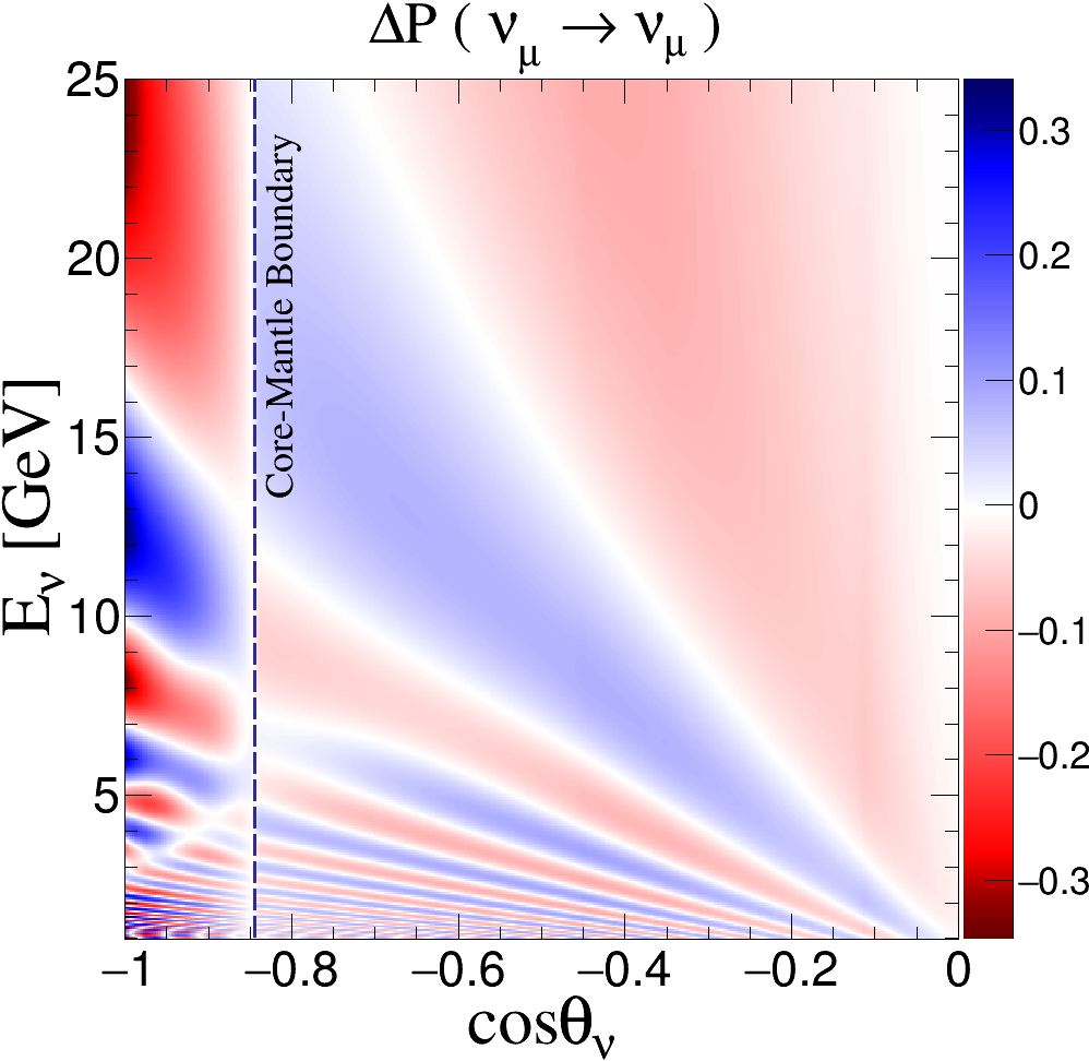
To illustrate this point, we first consider Earth as a uniform solid sphere of average mass density $\rho^{Earth}_{avg}\approx 5.5\,{\rm g/cm^{3}}$, which would give the corresponding value $\varepsilon_{\mu\tau}=0.0475$ for ${\text{a}}_{\mu\tau}=10^{-23}$ GeV, using Eq. (6). In Fig. 4, we show the difference $\Delta P$ between the probabilities predicted by these two scenarios, where we use three-flavor neutrino oscillation in the presence of matter effect considering the PREM profile of Earth. It is observed that for neutrinos that travel only through the mantle, i.e. for $\cos\theta_{\nu}\gtrsim-0.85$, we get $|\Delta P|\lesssim 0.1$. However, this difference grows for neutrinos passing through the core, reaching values as high as $|\Delta P|\approx 0.34$. Due to the significant $|\Delta P|$, the atmospheric neutrino data would be able to distinguish between the LV and NSI scenarios.

In this section, we explore the extent to which the LV vs. NSI discrimination is possible at the proposed 50 kt ICAL detector at INO. This detector would be sensitive to multi-GeV atmospheric $\nu_{\mu}$ and $\bar{\nu}_{\mu}$. It would detect muons in the energy range of 1 – 25 GeV with the energy resolution of 10 – 15% and zenith angle resolution of $<1^{\circ}$ for all but the almost-horizontal muons [110]. It would also measure the energy of hadron showers produced during atmospheric $\nu_{\mu}$ interaction events with a resolution of 35%–70% [111]. The magnetic field of 1.5 Tesla would give ICAL the unique capability of muon charge identification (CID), which in turn, would enable it to identify $\nu_{\mu}$ and $\bar{\nu}_{\mu}$ events separately with the CID efficiency of 98 – 99%, for muons beyond a few GeV to 50 GeV [110]. We simulate the events at the ICAL detector by using the NUANCE neutrino event generator [112] with the atmospheric neutrino flux from Ref. [113] to calculate the number of unoscillated events generated via the charged-current interactions. We incorporate the probabilities using the reweighting algorithm [114, 115]. We take into account the detector properties in the form of reconstruction efficiency, CID efficiency, and resolutions of muon energy, muon zenith angle and hadron energy, using the ICAL migration matrices [110, 111].

After an exposure of 1000 kt$\cdot$yr, about 8800 $\mu^{-}$ and 4000 $\mu^{+}$ reconstructed events are expected at ICAL. We use the reconstructed values of muon energy and zenith angle ($E_{\mu}^{\rm rec}$ and $\cos\theta_{\mu}^{\rm rec}$), along with hadron energy (${E^{\prime}}_{\rm had}^{\rm rec}$), as observables [116]. The analysis is carried out using fine bins in $\cos\theta_{\mu}^{\rm rec}$ for core-passing neutrinos [117]. The data is simulated using nonzero ${\text{a}}_{\mu\tau}^{\rm true}$, while the fit is attempted using nonzero $\varepsilon_{\mu\tau}^{\rm test}$. Using the frequentist approach, the median sensitivity of the detector to distinguish between LV and NSI scenarios, quantified by

is calculated with the Poissonian $\chi^{2}$ [118, 119] (see A for more details). We restrict the values of ${\text{a}}_{\mu\tau}$ and $\varepsilon_{\mu\tau}$ to be real. The five systematic uncertainties included are: 20% error in flux normalization, 10% error in cross section, 5% energy dependent tilt error in flux, 5% uncertainty on the zenith angle dependence of the flux, and 5% overall systematics for both $\nu_{\mu}$ and $\bar{\nu}_{\mu}$ events [120, 121, 114, 115, 116]. The oscillation parameters values given earlier in this study are taken to be fixed, since by the time 1000 kt$\cdot$yr data is available, the oscillation parameters would have been measured quite precisely. In Fig. 5, we show the best-fit values of $\varepsilon_{\mu\tau}^{\rm test}$ obtained for a range of ${\text{a}}_{\mu\tau}^{\rm true}$ values, and the $\Delta\chi^{2}$ at which the hypothesis of NSI can be rejected. The figure clearly brings out the advantage that CID provides: it enables the discrimination at the level of $\Delta\chi^{2}\approx 4$ for $|{\text{a}}_{\mu\tau}|\geq 0.5\times 10^{-23}$ GeV.

In Fig. 6, we quantify the extent to which an NSI interpretation would mimic, or fail to mimic, an actual LV scenario. We scan over a range of $\varepsilon_{\mu\tau}^{\rm test}$ for each value of ${\text{a}}_{\mu\tau}^{\rm true}$, and calculate the $\Delta\chi^{2}$ values. These values, in turn, indicate the confidence level (1 d.o.f.) at which the $\varepsilon_{\mu\tau}^{\rm test}$ would mimic a given value of ${\text{a}}_{\mu\tau}^{\rm true}$. The results in Fig. 6 can be interpreted as follows:

• 1.

  The points P1 and P2 lie on the line $\varepsilon_{\mu\tau}^{\rm test}$ = 0, i.e., the line which compares the SM against the LV scenarios. For these points, $\Delta\chi^{2}=3.84$. Thus, the points on this line to the left of P1 and the right of P2 indicate the values of ${\text{a}}_{\mu\tau}^{\rm true}$ for which the SM would be disfavored to more than 95% confidence level.

• 2.

  The points P3 and P4 lie on the line ${\text{a}}_{\mu\tau}^{\rm true}$ = 0, i.e., when there is no LV. For these points, $\Delta\chi^{2}=3.84$. Thus, in the no-BSM scenario, the NSI parameter $\varepsilon_{\mu\tau}^{\rm test}$ would be resticted to the segment P3–P4 at 95% confidence level.

• 3.

  The green-dashed diagonal line approximately passes through the best-fit values of $\varepsilon_{\mu\tau}^{\rm test}$. This line corresponds to eq. (6) with an average mass density of $\rho^{Earth}_{avg}\approx 5.5\,{\rm g/cm^{3}}$.

• 4.

  The points P5 and P6 on the diagonal line represent the values of ${\text{a}}_{\mu\tau}^{\rm true}$ beyond which any $\varepsilon_{\mu\tau}^{\rm test}$ would be ruled out to more than 95% confidence level.

• 5.

  The current experimental bounds on these BSM parameters from the IceCube experiment are $|{\text{a}}_{\mu\tau}|\leq 0.2\times 10^{-23}$ GeV [45] and $-\,0.0123\leq\varepsilon_{\mu\tau}\leq 0.0093$ [94] at 90% C.L., considering these new physics scenarios one-at-a-time. The shaded regions depict these allowed ranges.

As can be inferred from the figure, 1000 kt$\cdot$yr of ICAL data can distinguish between LV and NSI scenarios with up to 95% C.L. for $|{\text{a}}_{\mu\tau}^{\rm true}|\leq 0.5\times 10^{-23}$ GeV. In the scenarios with $|{\text{a}}_{\mu\tau}^{\rm true}|>0.2\times 10^{-23}$ GeV, these data can distinguish between LV and NSI to more than 68% confidence level. Higher exposure and the combination with data from other atmospheric neutrino experiments would enhance this sensitivity.

Future high-precision neutrino experiments may reveal the presence of new physics scenarios beyond oscillations. However, it is not enough to identify the presence of BSM physics; it is essential to identify its source and nature. In this work, we have pointed out for the first time that a long-baseline neutrino oscillation experiment cannot distinguish between the two popular BSM scenarios of LV and NSI. We have argued that the key to resolving this degeneracy is the observation of neutrinos passing through the core of Earth, and hence atmospheric neutrino experiments are critical for this purpose. We demonstrate that the ICAL experiment, that has excellent energy and directional resolutions for muons and can identify the muon charge, may be able to distinguish between these two scenarios. Using the detailed and rigorous simulation tools developed by the INO collaboration, we further estimate the sensitivity of the proposed ICAL detector for discriminating between the LV and NSI scenarios with 1000 kt$\cdot$yr exposure.

The analysis performed in this work can also be adapted for the currently running atmospheric neutrino experiments like Super-K, IceCube, DeepCore, ORCA, some of which also have sensitivity to electron events. The high-precision atmospheric neutrino data expected from the upcoming experiments like Hyper-K, DUNE and P-ONE will undoubtedly improve the prospects of the discrimination between LV and NSI scenarios.

We thank the members of the INO-ICAL collaboration for their valuable comments and constructive inputs. We sincerely thank A. Raychaudhuri and S. Uma Sankar for their careful reading of the manuscript and for providing useful suggestions. We thank V. A. Kosteleck$\acute{\rm y}$, P. Denton, and S. Palomares-Ruiz for their valuable comments. We acknowledge the support from the Department of Atomic Energy (DAE), Govt. of India, under the Project Identification Numbers RTI4002 and RIO 4001. S.K.A. is supported by the Young Scientist Project [INSA/SP/YSP/144/2017/1578] from the Indian National Science Academy (INSA). S.K.A. acknowledges the financial support from the Swarnajayanti Fellowship Research Grant (No. DST/SJF/PSA- 05/2019-20) provided by the Department of Science and Technology (DST), Govt. of India, and the Research Grant (File no. SB/SJF/2020-21/21) provided by the Science and Engineering Research Board (SERB) under the Swarnajayanti Fellowship by the DST, Govt. of India. S.K.A would like to thank the United States-India Educational Foundation for providing the financial support through the Fulbright-Nehru Academic and Professional Excellence Fellowship (Award No. 2710/F-N APE/2021). The numerical simulations are performed using the high-performance computing facilities CCHPC-19 and Sim01 at the Tata Institute of Fundamental Research (TIFR), Mumbai, India.

References

- Zyla et al. [2020] P. Zyla, et al. (Particle Data Group), Review of Particle Physics, PTEP 2020 (2020) 083C01. doi:10.1093/ptep/ptaa104, and 2021 update.
- Fukuda et al. [1999] Y. Fukuda, et al. (Super-Kamiokande), Constraints on neutrino oscillation parameters from the measurement of day night solar neutrino fluxes at Super-Kamiokande, Phys. Rev. Lett. 82 (1999) 1810–1814. doi:10.1103/PhysRevLett.82.1810. arXiv:hep-ex/9812009.
- Fukuda et al. [2001] S. Fukuda, et al. (Super-Kamiokande), Constraints on neutrino oscillations using 1258 days of Super-Kamiokande solar neutrino data, Phys. Rev. Lett. 86 (2001) 5656–5660. doi:10.1103/PhysRevLett.86.5656. arXiv:hep-ex/0103033.
- Ahmad et al. [2001] Q. R. Ahmad, et al. (SNO), Measurement of the rate of interactions produced by 8B solar neutrinos at the Sudbury Neutrino Observatory, Phys. Rev. Lett. 87 (2001) 071301. doi:10.1103/PhysRevLett.87.071301. arXiv:nucl-ex/0106015.
- Fukuda et al. [2002] S. Fukuda, et al. (Super-Kamiokande), Determination of solar neutrino oscillation parameters using 1496 days of Super-Kamiokande I data, Phys. Lett. B 539 (2002) 179–187. doi:10.1016/S0370-2693(02)02090-7. arXiv:hep-ex/0205075.
- Hosaka et al. [2006] J. Hosaka, et al. (Super-Kamiokande), Solar neutrino measurements in super-Kamiokande-I, Phys. Rev. D 73 (2006) 112001. doi:10.1103/PhysRevD.73.112001. arXiv:hep-ex/0508053.
- Cravens et al. [2008] J. P. Cravens, et al. (Super-Kamiokande), Solar neutrino measurements in Super-Kamiokande-II, Phys. Rev. D 78 (2008) 032002. doi:10.1103/PhysRevD.78.032002. arXiv:0803.4312.
- Abe et al. [2011] K. Abe, et al. (Super-Kamiokande), Solar neutrino results in Super-Kamiokande-III, Phys. Rev. D 83 (2011) 052010. doi:10.1103/PhysRevD.83.052010. arXiv:1010.0118.
- Aharmim et al. [2013] B. Aharmim, et al. (SNO), Combined Analysis of all Three Phases of Solar Neutrino Data from the Sudbury Neutrino Observatory, Phys. Rev. C 88 (2013) 025501. doi:10.1103/PhysRevC.88.025501. arXiv:1109.0763.
- Achar et al. [1965] C. V. Achar, et al., Detection of muons produced by cosmic ray neutrinos deep underground, Phys. Lett. 18 (1965) 196–199. doi:10.1016/0031-9163(65)90712-2.
- Fukuda et al. [1998] Y. Fukuda, et al. (Super-Kamiokande), Evidence for oscillation of atmospheric neutrinos, Phys. Rev. Lett. 81 (1998) 1562. doi:10.1103/PhysRevLett.81.1562. arXiv:hep-ex/9807003.
- Ashie et al. [2004] Y. Ashie, et al. (Super-Kamiokande), Evidence for an oscillatory signature in atmospheric neutrino oscillation, Phys. Rev. Lett. 93 (2004) 101801. doi:10.1103/PhysRevLett.93.101801. arXiv:hep-ex/0404034.
- Aartsen et al. [2015] M. G. Aartsen, et al. (IceCube), Determining neutrino oscillation parameters from atmospheric muon neutrino disappearance with three years of IceCube DeepCore data, Phys. Rev. D 91 (2015) 072004. doi:10.1103/PhysRevD.91.072004. arXiv:1410.7227.
- Abe et al. [2018] K. Abe, et al. (Super-Kamiokande), Atmospheric neutrino oscillation analysis with external constraints in Super-Kamiokande I-IV, Phys. Rev. D 97 (2018) 072001. doi:10.1103/PhysRevD.97.072001. arXiv:1710.09126.
- Eguchi et al. [2003] K. Eguchi, et al. (KamLAND), First results from KamLAND: Evidence for reactor anti-neutrino disappearance, Phys. Rev. Lett. 90 (2003) 021802. doi:10.1103/PhysRevLett.90.021802. arXiv:hep-ex/0212021.
- Araki et al. [2005] T. Araki, et al. (KamLAND Collaboration), Measurement of neutrino oscillation with KamLAND: Evidence of spectral distortion, Phys.Rev.Lett. 94 (2005) 081801. doi:10.1103/PhysRevLett.94.081801. arXiv:hep-ex/0406035.
- An et al. [2012] F. P. An, et al. (Daya Bay), Observation of electron-antineutrino disappearance at Daya Bay, Phys. Rev. Lett. 108 (2012) 171803. doi:10.1103/PhysRevLett.108.171803. arXiv:1203.1669.
- Ahn et al. [2012] J. K. Ahn, et al. (RENO), Observation of Reactor Electron Antineutrino Disappearance in the RENO Experiment, Phys. Rev. Lett. 108 (2012) 191802. doi:10.1103/PhysRevLett.108.191802. arXiv:1204.0626.
- Gando et al. [2013] A. Gando, et al. (KamLAND), Reactor On-Off Antineutrino Measurement with KamLAND, Phys. Rev. D 88 (2013) 033001. doi:10.1103/PhysRevD.88.033001. arXiv:1303.4667.
- Bak et al. [2018] G. Bak, et al. (RENO), Measurement of Reactor Antineutrino Oscillation Amplitude and Frequency at RENO, Phys. Rev. Lett. 121 (2018) 201801. doi:10.1103/PhysRevLett.121.201801. arXiv:1806.00248.
- Adey et al. [2018] D. Adey, et al. (Daya Bay), Measurement of the Electron Antineutrino Oscillation with 1958 Days of Operation at Daya Bay, Phys. Rev. Lett. 121 (2018) 241805. doi:10.1103/PhysRevLett.121.241805. arXiv:1809.02261.
- de Kerret et al. [2020] H. de Kerret, et al. (Double Chooz), Double Chooz measurement via total neutron capture detection, Nature Phys. 16 (2020) 558–564. doi:10.1038/s41567-020-0831-y. arXiv:1901.09445.
- Aliu et al. [2005] E. Aliu, et al. (K2K), Evidence for muon neutrino oscillation in an accelerator-based experiment, Phys. Rev. Lett. 94 (2005) 081802. doi:10.1103/PhysRevLett.94.081802. arXiv:hep-ex/0411038.
- Adamson et al. [2008] P. Adamson, et al. (MINOS), Measurement of Neutrino Oscillations with the MINOS Detectors in the NuMI Beam, Phys.Rev.Lett. 101 (2008) 131802. doi:10.1103/PhysRevLett.101.131802. arXiv:0806.2237.
- Adamson et al. [2013a] P. Adamson, et al. (MINOS), Electron neutrino and antineutrino appearance in the full MINOS data sample, Phys. Rev. Lett. 110 (2013a) 171801. doi:10.1103/PhysRevLett.110.171801. arXiv:1301.4581.
- Adamson et al. [2013b] P. Adamson, et al. (MINOS), Measurement of Neutrino and Antineutrino Oscillations Using Beam and Atmospheric Data in MINOS, Phys. Rev. Lett. 110 (2013b) 251801. doi:10.1103/PhysRevLett.110.251801. arXiv:1304.6335.
- Abe et al. [2020] K. Abe, et al. (T2K), Constraint on the matter–antimatter symmetry-violating phase in neutrino oscillations, Nature 580 (2020) 339–344. doi:10.1038/s41586-020-2177-0. arXiv:1910.03887, [Erratum: Nature 583, E16 (2020)].
- Acero et al. [2019] M. A. Acero, et al. (NOvA), First Measurement of Neutrino Oscillation Parameters using Neutrinos and Antineutrinos by NOvA, Phys. Rev. Lett. 123 (2019) 151803. doi:10.1103/PhysRevLett.123.151803. arXiv:1906.04907.
- Argüelles et al. [2020] C. A. Argüelles, et al., New opportunities at the next-generation neutrino experiments I: BSM neutrino physics and dark matter, Rept. Prog. Phys. 83 (2020) 124201. doi:10.1088/1361-6633/ab9d12. arXiv:1907.08311.
- Colladay and Kostelecky [1997] D. Colladay, V. A. Kostelecky, CPT violation and the standard model, Phys. Rev. D 55 (1997) 6760–6774. doi:10.1103/PhysRevD.55.6760. arXiv:hep-ph/9703464.
- Auerbach et al. [2005] L. B. Auerbach, et al. (LSND), Tests of Lorentz violation in anti-nu(mu) — anti-nu(e) oscillations, Phys. Rev. D 72 (2005) 076004. doi:10.1103/PhysRevD.72.076004. arXiv:hep-ex/0506067.
- Adamson et al. [2008] P. Adamson, et al. (MINOS), Testing Lorentz Invariance and CPT Conservation with NuMI Neutrinos in the MINOS Near Detector, Phys. Rev. Lett. 101 (2008) 151601. doi:10.1103/PhysRevLett.101.151601. arXiv:0806.4945.
- Adamson et al. [2010] P. Adamson, et al. (MINOS), A Search for Lorentz Invariance and CPT Violation with the MINOS Far Detector, Phys. Rev. Lett. 105 (2010) 151601. doi:10.1103/PhysRevLett.105.151601. arXiv:1007.2791.
- Abbasi et al. [2010] R. Abbasi, et al. (IceCube), Search for a Lorentz-violating sidereal signal with atmospheric neutrinos in IceCube, Phys. Rev. D 82 (2010) 112003. doi:10.1103/PhysRevD.82.112003. arXiv:1010.4096.
- Aguilar-Arevalo et al. [2013] A. A. Aguilar-Arevalo, et al. (MiniBooNE), Test of Lorentz and CPT violation with Short Baseline Neutrino Oscillation Excesses, Phys. Lett. B 718 (2013) 1303–1308. doi:10.1016/j.physletb.2012.12.020. arXiv:1109.3480.
- Kostelecký and Russell [2011] V. A. Kostelecký, N. Russell, Data tables for lorentz and violation, Rev. Mod. Phys. 83 (2011) 11–31. URL: https://link.aps.org/doi/10.1103/RevModPhys.83.11. doi:10.1103/RevModPhys.83.11.
- Adamson et al. [2012] P. Adamson, et al. (MINOS), Search for Lorentz invariance and CPT violation with muon antineutrinos in the MINOS Near Detector, Phys. Rev. D 85 (2012) 031101. doi:10.1103/PhysRevD.85.031101. arXiv:1201.2631.
- Abe et al. [2012] Y. Abe, et al. (Double Chooz), First Test of Lorentz Violation with a Reactor-based Antineutrino Experiment, Phys. Rev. D 86 (2012) 112009. doi:10.1103/PhysRevD.86.112009. arXiv:1209.5810.
- Rebel and Mufson [2013] B. Rebel, S. Mufson, The Search for Neutrino-Antineutrino Mixing Resulting from Lorentz Invariance Violation using neutrino interactions in MINOS, Astropart. Phys. 48 (2013) 78–81. doi:10.1016/j.astropartphys.2013.07.006. arXiv:1301.4684.
- Díaz et al. [2013] J. S. Díaz, T. Katori, J. Spitz, J. M. Conrad, Search for neutrino-antineutrino oscillations with a reactor experiment, Phys. Lett. B 727 (2013) 412–416. doi:10.1016/j.physletb.2013.10.058. arXiv:1307.5789.
- Diaz and Schwetz [2016] J. S. Diaz, T. Schwetz, Limits on CPT violation from solar neutrinos, Phys. Rev. D 93 (2016) 093004. doi:10.1103/PhysRevD.93.093004. arXiv:1603.04468.
- Abe et al. [2015] K. Abe, et al. (Super-Kamiokande), Test of Lorentz invariance with atmospheric neutrinos, Phys. Rev. D 91 (2015) 052003. doi:10.1103/PhysRevD.91.052003. arXiv:1410.4267.
- Abe et al. [2017] K. Abe, et al. (T2K), Search for Lorentz and CPT violation using sidereal time dependence of neutrino flavor transitions over a short baseline, Phys. Rev. D 95 (2017) 111101. doi:10.1103/PhysRevD.95.111101. arXiv:1703.01361.
- Adey et al. [2018] D. Adey, et al. (Daya Bay), Search for a time-varying electron antineutrino signal at Daya Bay, Phys. Rev. D 98 (2018) 092013. doi:10.1103/PhysRevD.98.092013. arXiv:1809.04660.
- Aartsen et al. [2018] M. G. Aartsen, et al. (IceCube), Neutrino Interferometry for High-Precision Tests of Lorentz Symmetry with IceCube, Nature Phys. 14 (2018) 961–966. doi:10.1038/s41567-018-0172-2. arXiv:1709.03434.
- Sahoo et al. [2022] S. Sahoo, A. Kumar, S. K. Agarwalla, Probing Lorentz Invariance Violation with atmospheric neutrinos at INO-ICAL, JHEP 03 (2022) 050. doi:10.1007/JHEP03(2022)050. arXiv:2110.13207.
- Wolfenstein [1978] L. Wolfenstein, Neutrino oscillations in matter, Phys. Rev. D 17 (1978) 2369–2374. URL: https://link.aps.org/doi/10.1103/PhysRevD.17.2369. doi:10.1103/PhysRevD.17.2369.
- Ohlsson [2013] T. Ohlsson, Status of non-standard neutrino interactions, Rept. Prog. Phys. 76 (2013) 044201. doi:10.1088/0034-4885/76/4/044201. arXiv:1209.2710.
- Fornengo et al. [2002] N. Fornengo, M. Maltoni, R. Tomas, J. W. F. Valle, Probing neutrino nonstandard interactions with atmospheric neutrino data, Phys. Rev. D 65 (2002) 013010. doi:10.1103/PhysRevD.65.013010. arXiv:hep-ph/0108043.
- Kopp et al. [2010] J. Kopp, P. A. N. Machado, S. J. Parke, Interpretation of MINOS Data in Terms of Non-Standard Neutrino Interactions, Phys. Rev. D 82 (2010) 113002. doi:10.1103/PhysRevD.82.113002. arXiv:1009.0014.
- Mitsuka et al. [2011] G. Mitsuka, et al. (Super-Kamiokande), Study of Non-Standard Neutrino Interactions with Atmospheric Neutrino Data in Super-Kamiokande I and II, Phys. Rev. D 84 (2011) 113008. doi:10.1103/PhysRevD.84.113008. arXiv:1109.1889.
- Choubey et al. [2015] S. Choubey, A. Ghosh, T. Ohlsson, D. Tiwari, Neutrino Physics with Non-Standard Interactions at INO, JHEP 12 (2015) 126. doi:10.1007/JHEP12(2015)126. arXiv:1507.02211.
- Salvado et al. [2017] J. Salvado, O. Mena, S. Palomares-Ruiz, N. Rius, Non-standard interactions with high-energy atmospheric neutrinos at IceCube, JHEP 01 (2017) 141. doi:10.1007/JHEP01(2017)141. arXiv:1609.03450.
- Aartsen et al. [2018] M. G. Aartsen, et al. (IceCube), Search for Nonstandard Neutrino Interactions with IceCube DeepCore, Phys. Rev. D 97 (2018) 072009. doi:10.1103/PhysRevD.97.072009. arXiv:1709.07079.
- Farzan and Tortola [2018] Y. Farzan, M. Tortola, Neutrino oscillations and Non-Standard Interactions, Front.in Phys. 6 (2018) 10. doi:10.3389/fphy.2018.00010. arXiv:1710.09360.
- Khatun et al. [2020] A. Khatun, S. S. Chatterjee, T. Thakore, S. K. Agarwalla, Enhancing sensitivity to non-standard neutrino interactions at INO combining muon and hadron information, Eur. Phys. J. C 80 (2020) 533. doi:10.1140/epjc/s10052-020-8097-1. arXiv:1907.02027.
- Kumar et al. [2021] A. Kumar, A. Khatun, S. K. Agarwalla, A. Dighe, A New Approach to Probe Non-Standard Interactions in Atmospheric Neutrino Experiments, JHEP 04 (2021) 159. doi:10.1007/JHEP04(2021)159. arXiv:2101.02607.
- Hernández Rey et al. [2021] J. J. Hernández Rey, N. R. Khan Chowdhury, J. Manczak, S. Navas, J. D. Zornoza (ANTARES, KM3NeT), Search for neutrino non-standard interactions with ANTARES and KM3NeT-ORCA, in: 9th Very Large Volume Neutrino Telescopes Workshop 2021, 2021. arXiv:2107.14296.
- Abbasi et al. [2021] R. Abbasi, et al. ((IceCube Collaboration)*, IceCube), All-flavor constraints on nonstandard neutrino interactions and generalized matter potential with three years of IceCube DeepCore data, Phys. Rev. D 104 (2021) 072006. doi:10.1103/PhysRevD.104.072006. arXiv:2106.07755.
- Albert et al. [2021] A. Albert, et al. (ANTARES), Search for non-standard neutrino interactions with 10 years of ANTARES data (2021). arXiv:2112.14517.
- Denton and Pestes [2021] P. B. Denton, R. Pestes, Neutrino oscillations through the Earth’s core, Phys. Rev. D 104 (2021) 113007. doi:10.1103/PhysRevD.104.113007. arXiv:2110.01148.
- Ahmed et al. [2017] S. Ahmed, et al. (ICAL), Physics Potential of the ICAL detector at the India-based Neutrino Observatory (INO), Pramana 88 (2017) 79. doi:10.1007/s12043-017-1373-4. arXiv:1505.07380.
- Polyakov [1987] A. M. Polyakov, Gauge Fields and Strings, volume 3 of Contemporary concepts in physics, Harwood Academic Publishers, 1987.
- Kostelecky and Samuel [1989a] V. A. Kostelecky, S. Samuel, Spontaneous Breaking of Lorentz Symmetry in String Theory, Phys. Rev. D 39 (1989a) 683. doi:10.1103/PhysRevD.39.683.
- Kostelecky and Samuel [1989b] V. A. Kostelecky, S. Samuel, Phenomenological Gravitational Constraints on Strings and Higher Dimensional Theories, Phys. Rev. Lett. 63 (1989b) 224. doi:10.1103/PhysRevLett.63.224.
- Kostelecký and Samuel [1991] V. A. Kostelecký, S. Samuel, Photon and graviton masses in string theories, Phys. Rev. Lett. 66 (1991) 1811–1814. URL: https://link.aps.org/doi/10.1103/PhysRevLett.66.1811. doi:10.1103/PhysRevLett.66.1811.
- Kostelecky and Potting [1991] V. A. Kostelecky, R. Potting, CPT and strings, Nucl. Phys. B 359 (1991) 545–570. doi:10.1016/0550-3213(91)90071-5.
- Kostelecky and Potting [1996] V. A. Kostelecky, R. Potting, Expectation values, Lorentz invariance, and CPT in the open bosonic string, Phys. Lett. B 381 (1996) 89–96. doi:10.1016/0370-2693(96)00589-8. arXiv:hep-th/9605088.
- Kostelecky et al. [2000] V. A. Kostelecky, M. Perry, R. Potting, Off-shell structure of the string sigma model, Phys. Rev. Lett. 84 (2000) 4541–4544. doi:10.1103/PhysRevLett.84.4541. arXiv:hep-th/9912243.
- Kostelecky and Potting [2001] V. A. Kostelecky, R. Potting, Analytical construction of a nonperturbative vacuum for the open bosonic string, Phys. Rev. D 63 (2001) 046007. doi:10.1103/PhysRevD.63.046007. arXiv:hep-th/0008252.
- Gambini and Pullin [1999] R. Gambini, J. Pullin, Nonstandard optics from quantum space-time, Phys. Rev. D 59 (1999) 124021. doi:10.1103/PhysRevD.59.124021. arXiv:gr-qc/9809038.
- Alfaro et al. [2002] J. Alfaro, H. A. Morales-Tecotl, L. F. Urrutia, Quantum gravity and spin 1/2 particles effective dynamics, Phys. Rev. D 66 (2002) 124006. doi:10.1103/PhysRevD.66.124006. arXiv:hep-th/0208192.
- Sudarsky et al. [2002] D. Sudarsky, L. Urrutia, H. Vucetich, New observational bounds to quantum gravity signals, Phys. Rev. Lett. 89 (2002) 231301. doi:10.1103/PhysRevLett.89.231301. arXiv:gr-qc/0204027.
- Amelino-Camelia [2002] G. Amelino-Camelia, Quantum gravity phenomenology: Status and prospects, Mod. Phys. Lett. A 17 (2002) 899–922. doi:10.1142/S0217732302007612. arXiv:gr-qc/0204051.
- Ng [2003] Y. J. Ng, Selected topics in Planck scale physics, Mod. Phys. Lett. A 18 (2003) 1073–1098. doi:10.1142/S0217732303010934. arXiv:gr-qc/0305019.
- Kostelecky and Mewes [2012] A. Kostelecky, M. Mewes, Neutrinos with Lorentz-violating operators of arbitrary dimension, Phys. Rev. D 85 (2012) 096005. doi:10.1103/PhysRevD.85.096005. arXiv:1112.6395.
- Barenboim et al. [2019] G. Barenboim, M. Masud, C. A. Ternes, M. Tórtola, Exploring the intrinsic Lorentz-violating parameters at DUNE, Phys. Lett. B 788 (2019) 308–315. doi:10.1016/j.physletb.2018.11.040. arXiv:1805.11094.
- Kostelecky and Mewes [2004] V. A. Kostelecky, M. Mewes, Lorentz and CPT violation in neutrinos, Phys. Rev. D 69 (2004) 016005. doi:10.1103/PhysRevD.69.016005. arXiv:hep-ph/0309025.
- Greenberg [2002] O. W. Greenberg, CPT violation implies violation of Lorentz invariance, Phys. Rev. Lett. 89 (2002) 231602. doi:10.1103/PhysRevLett.89.231602. arXiv:hep-ph/0201258.
- Appelquist and Carazzone [1975] T. Appelquist, J. Carazzone, Infrared Singularities and Massive Fields, Phys. Rev. D 11 (1975) 2856. doi:10.1103/PhysRevD.11.2856.
- Colladay and Kostelecky [1998] D. Colladay, V. A. Kostelecky, Lorentz violating extension of the standard model, Phys. Rev. D 58 (1998) 116002. doi:10.1103/PhysRevD.58.116002. arXiv:hep-ph/9809521.
- Kostelecky and Lehnert [2001] V. A. Kostelecky, R. Lehnert, Stability, causality, and Lorentz and CPT violation, Phys. Rev. D 63 (2001) 065008. doi:10.1103/PhysRevD.63.065008. arXiv:hep-th/0012060.
- Kostelecky [2004] V. A. Kostelecky, Gravity, Lorentz violation, and the standard model, Phys. Rev. D 69 (2004) 105009. doi:10.1103/PhysRevD.69.105009. arXiv:hep-th/0312310.
- Bluhm [2006] R. Bluhm, Overview of the SME: Implications and phenomenology of Lorentz violation, Lect. Notes Phys. 702 (2006) 191–226. doi:10.1007/3-540-34523-X_8. arXiv:hep-ph/0506054.
- Jacobson and Ohlsson [2004] M. Jacobson, T. Ohlsson, Extrinsic CPT violation in neutrino oscillations in matter, Phys. Rev. D 69 (2004) 013003. doi:10.1103/PhysRevD.69.013003. arXiv:hep-ph/0305064.
- Ohlsson and Zhou [2015] T. Ohlsson, S. Zhou, Extrinsic and Intrinsic CPT Asymmetries in Neutrino Oscillations, Nucl. Phys. B 893 (2015) 482–500. doi:10.1016/j.nuclphysb.2015.02.015. arXiv:1408.4722.
- Kopp et al. [2008] J. Kopp, M. Lindner, T. Ota, J. Sato, Non-standard neutrino interactions in reactor and superbeam experiments, Phys. Rev. D 77 (2008) 013007. doi:10.1103/PhysRevD.77.013007. arXiv:0708.0152.
- Kumar et al. [2021] A. Kumar, A. Khatun, S. K. Agarwalla, A. Dighe, From oscillation dip to oscillation valley in atmospheric neutrino experiments, Eur. Phys. J. C 81 (2021) 190. doi:10.1140/epjc/s10052-021-08946-8. arXiv:2006.14529.
- NuF [2020] Nufit 5.0, 2020. URL: http://www.nu-fit.org.
- Esteban et al. [2020] I. Esteban, M. C. Gonzalez-Garcia, M. Maltoni, T. Schwetz, A. Zhou, The fate of hints: updated global analysis of three-flavor neutrino oscillations, JHEP 09 (2020) 178. doi:10.1007/JHEP09(2020)178. arXiv:2007.14792.
- de Salas et al. [2021] P. F. de Salas, D. V. Forero, S. Gariazzo, P. Martínez-Miravé, O. Mena, C. A. Ternes, M. Tórtola, J. W. F. Valle, 2020 global reassessment of the neutrino oscillation picture, JHEP 02 (2021) 071. doi:10.1007/JHEP02(2021)071. arXiv:2006.11237.
- Dziewonski and Anderson [1981] A. Dziewonski, D. Anderson, Preliminary Reference Earth Model, Phys.Earth Planet.Interiors 25 (1981) 297–356. doi:10.1016/0031-9201(81)90046-7.
- Weinberg [1979] S. Weinberg, Baryon and Lepton Nonconserving Processes, Phys. Rev. Lett. 43 (1979) 1566–1570. doi:10.1103/PhysRevLett.43.1566.
- Abbasi et al. [2022] R. Abbasi, et al. (IceCube), Strong Constraints on Neutrino Nonstandard Interactions from TeV-Scale Disappearance at IceCube, Phys. Rev. Lett. 129 (2022) 011804. doi:10.1103/PhysRevLett.129.011804. arXiv:2201.03566.
- Diaz [2015] J. S. Diaz, Correspondence between nonstandard interactions and CPT violation in neutrino oscillations (2015). arXiv:1506.01936.
- Agarwalla and Masud [2020] S. K. Agarwalla, M. Masud, Can Lorentz invariance violation affect the sensitivity of deep underground neutrino experiment?, Eur. Phys. J. C 80 (2020) 716. doi:10.1140/epjc/s10052-020-8303-1. arXiv:1912.13306.
- Gandhi et al. [2006] R. Gandhi, P. Ghoshal, S. Goswami, P. Mehta, S. U. Sankar, Earth matter effects at very long baselines and the neutrino mass hierarchy, Phys. Rev. D 73 (2006) 053001. doi:10.1103/PhysRevD.73.053001. arXiv:hep-ph/0411252.
- Agarwalla [2008] S. K. Agarwalla, Some Aspects of Neutrino Mixing and Oscillations, Ph.D. thesis, Calcutta U., 2008. arXiv:0908.4267.
- Roe [2017] B. Roe, Matter density versus distance for the neutrino beam from Fermilab to Lead, South Dakota, and comparison of oscillations with variable and constant density, Phys. Rev. D 95 (2017) 113004. doi:10.1103/PhysRevD.95.113004. arXiv:1707.02322.
- Abi et al. [2021] B. Abi, et al. (DUNE), Experiment Simulation Configurations Approximating DUNE TDR (2021). arXiv:2103.04797.
- Mikheev and Smirnov [1985] S. P. Mikheev, A. Y. Smirnov, Resonance enhancement of oscillations in matter and solar neutrino spectroscopy, Sov. J. Nucl. Phys. 42 (1985) 913. [Yad.Fiz.42:1441-1448,1985].
- Mikheev and Smirnov [1986] S. Mikheev, A. Y. Smirnov, Resonant amplification of neutrino oscillations in matter and solar neutrino spectroscopy, Nuovo Cim. C9 (1986) 17. doi:10.1007/BF02508049.
- Petcov [1998] S. Petcov, Diffractive - like (or parametric resonance - like?) enhancement of the earth (day - night) effect for solar neutrinos crossing the earth core, Phys. Lett. B 434 (1998) 321. doi:10.1016/S0370-2693(98)00742-4. arXiv:hep-ph/9805262.
- Chizhov et al. [1998] M. Chizhov, M. Maris, S. T. Petcov, On the oscillation length resonance in the transitions of solar and atmospheric neutrinos crossing the earth core (1998). arXiv:hep-ph/9810501.
- Petcov [1999] S. T. Petcov, New enhancement mechanism of the transitions in the earth of the solar and atmospheric neutrinos crossing the earth core, Nucl. Phys. B Proc. Suppl. 77 (1999) 93–97. doi:10.1016/S0920-5632(99)00403-X. arXiv:hep-ph/9809587.
- Chizhov and Petcov [1999] M. Chizhov, S. Petcov, New conditions for a total neutrino conversion in a medium, Phys.Rev.Lett. 83 (1999) 1096–1099. doi:10.1103/PhysRevLett.83.1096. arXiv:hep-ph/9903399.
- Chizhov and Petcov [2001] M. V. Chizhov, S. T. Petcov, Enhancing mechanisms of neutrino transitions in a medium of nonperiodic constant density layers and in the earth, Phys. Rev. D 63 (2001) 073003. doi:10.1103/PhysRevD.63.073003. arXiv:hep-ph/9903424.
- Akhmedov [1999] E. K. Akhmedov, Parametric resonance of neutrino oscillations and passage of solar and atmospheric neutrinos through the earth, Nucl. Phys. B538 (1999) 25. doi:10.1016/S0550-3213(98)00723-8. arXiv:hep-ph/9805272.
- Akhmedov et al. [1999] E. K. Akhmedov, A. Dighe, P. Lipari, A. Smirnov, Atmospheric neutrinos at Super-Kamiokande and parametric resonance in neutrino oscillations, Nucl. Phys. B542 (1999) 3. doi:10.1016/S0550-3213(98)00825-6. arXiv:hep-ph/9808270.
- Chatterjee et al. [2014] A. Chatterjee, K. Meghna, K. Rawat, T. Thakore, V. Bhatnagar, et al., A Simulations Study of the Muon Response of the Iron Calorimeter Detector at the India-based Neutrino Observatory, JINST 9 (2014) P07001. doi:10.1088/1748-0221/9/07/P07001. arXiv:1405.7243.
- Devi et al. [2013] M. M. Devi, A. Ghosh, D. Kaur, L. S. Mohan, S. Choubey, et al., Hadron energy response of the Iron Calorimeter detector at the India-based Neutrino Observatory, JINST 8 (2013) P11003. doi:10.1088/1748-0221/8/11/P11003. arXiv:1304.5115.
- Casper [2002] D. Casper, The Nuance neutrino physics simulation, and the future, Nucl. Phys. Proc. Suppl. 112 (2002) 161. doi:10.1016/S0920-5632(02)01756-5. arXiv:hep-ph/0208030.
- Honda et al. [2015] M. Honda, M. Sajjad Athar, T. Kajita, K. Kasahara, S. Midorikawa, Atmospheric neutrino flux calculation using the NRLMSISE-00 atmospheric model, Phys. Rev. D 92 (2015) 023004. doi:10.1103/PhysRevD.92.023004. arXiv:1502.03916.
- Ghosh et al. [2013] A. Ghosh, T. Thakore, S. Choubey, Determining the Neutrino Mass Hierarchy with INO, T2K, NOvA and Reactor Experiments, JHEP 1304 (2013) 009. doi:10.1007/JHEP04(2013)009. arXiv:1212.1305.
- Thakore et al. [2013] T. Thakore, A. Ghosh, S. Choubey, A. Dighe, The Reach of INO for Atmospheric Neutrino Oscillation Parameters, JHEP 1305 (2013) 058. doi:10.1007/JHEP05(2013)058. arXiv:1303.2534.
- Devi et al. [2014] M. M. Devi, T. Thakore, S. K. Agarwalla, A. Dighe, Enhancing sensitivity to neutrino parameters at INO combining muon and hadron information, JHEP 10 (2014) 189. doi:10.1007/JHEP10(2014)189. arXiv:1406.3689.
- Upadhyay et al. [2022] A. K. Upadhyay, A. Kumar, S. K. Agarwalla, A. Dighe, Locating the Core-Mantle Boundary using Oscillations of Atmospheric Neutrinos (2022). arXiv:2211.08688.
- Baker and Cousins [1984] S. Baker, R. D. Cousins, Clarification of the Use of Chi Square and Likelihood Functions in Fits to Histograms, Nucl. Instrum. Meth. 221 (1984) 437–442. doi:10.1016/0167-5087(84)90016-4.
- Blennow et al. [2014] M. Blennow, P. Coloma, P. Huber, T. Schwetz, Quantifying the sensitivity of oscillation experiments to the neutrino mass ordering, JHEP 1403 (2014) 028. doi:10.1007/JHEP03(2014)028. arXiv:1311.1822.
- Kameda [2002] J. Kameda, Detailed studies of neutrino oscillations with atmospheric neutrinos of wide energy range from 100 MeV to 1000 GeV in Super-Kamiokande, Ph.D. thesis, Tokyo U., 2002.
- Gonzalez-Garcia and Maltoni [2004a] M. C. Gonzalez-Garcia, M. Maltoni, Atmospheric neutrino oscillations and new physics, Phys. Rev. D 70 (2004a) 033010. doi:10.1103/PhysRevD.70.033010. arXiv:hep-ph/0404085.
- Gonzalez-Garcia and Maltoni [2004b] M. C. Gonzalez-Garcia, M. Maltoni, Atmospheric neutrino oscillations and new physics, Phys. Rev. D70 (2004b) 033010. doi:10.1103/PhysRevD.70.033010. arXiv:hep-ph/0404085.
- Huber et al. [2002] P. Huber, M. Lindner, W. Winter, Superbeams versus neutrino factories, Nucl. Phys. B645 (2002) 3–48. doi:10.1016/S0550-3213(02)00825-8. arXiv:hep-ph/0204352.
- Fogli et al. [2002] G. L. Fogli, E. Lisi, A. Marrone, D. Montanino, A. Palazzo, Getting the most from the statistical analysis of solar neutrino oscillations, Phys. Rev. D 66 (2002) 053010. doi:10.1103/PhysRevD.66.053010. arXiv:hep-ph/0206162.