Augmented Transition Path Theory for Sequences of Events
Abstract
Transition path theory provides a statistical description of the dynamics of a reaction in terms of local spatial quantities. In its original formulation, it is limited to reactions that consist of trajectories flowing from a reactant set to a product set . We extend the basic concepts and principles of transition path theory to reactions in which trajectories exhibit a specified sequence of events and illustrate the utility of this generalization on examples.
I Introduction
Many reactions studied today proceed through competing pathways. Understanding such reactions relies on being able to assess the relative importance of the competing pathways and how they contribute to overall rates. When the pathways are well separated, they can be treated independently, often by traditional theories that assume a well-defined activated complex (transition state) and a simple form for the underlying (free) energy landscape governing the dynamics Hänggi, Talkner, and Borkovec 1990; Peters 2017. However, when the (observed) dynamics are stochastic, the pathways of reactions often overlap in configuration space. Approaches that treat competing pathways in a unified fashion are thus needed.
To this end, here, we build on transition path theory (TPT) E and Vanden-Eijnden 2006; Vanden-Eijnden 2006; E and Vanden-Eijnden 2010; Metzner, Schütte, and Vanden-Eijnden 2009; Metzner, Schütte, and Vanden-Eijnden 2006. The core idea of transition path theory is that the statistics of the ensemble of reactive trajectories can be related to quantities that are local in space: probability currents of reactive trajectories (henceforth, reactive currents) and committors. These quantities enable TPT to go beyond traditional theories by providing information about mechanisms. Reactive currents quantify flows in phase space. Committors, which are probabilities of reaching one metastable state before another, by definition characterize the progress of stochastic reactions Du et al. 1998.
In its traditional formulation, TPT focuses on transitions between two metastable states. In the present paper, we extend TPT to compute statistics for sequences of events, and we show how this significantly expands its applicability. Our work builds on but goes beyond previous studies. It is closely related to history-augmented Markov state models, in which states are labeled based on the last metastable state visited Suárez, Adelman, and Zuckerman 2016. Separating the ensemble of reactive trajectories using these labels enables rates to be computed from the flux into a metastable state Vanden-Eijnden and Venturoli 2009; Dickson, Warmflash, and Dinner 2009, as well as reactive currents and committors from the underlying trajectories Vani, Weare, and Dinner 2022. Our approach generalizes the labeling strategy to sequences of arbitrary numbers of states and allows specification of not just past events but also future ones.
Our work also has connections to that of Koltai and co-workers, who extended TPT to allow trajectories to leave and enter the region connecting the metastable states to analyze trajectory segments from satellite data for drifters in the ocean Miron et al. 2021. Specifically, they redefined committors to exclude trajectories that were not wholly within this region and noted that this approach could be used to exclude trajectories that pass through selected states. They also considered computing statistics for trajectories beginning and ending in specific portions of metastable states. Both of these developments allow statistics to be computed for subsets of reactive trajectories based on the states that they visit.
We present our work as follows. First, in Sections II.1 and II.2, we review how TPT expresses path statistics in terms of spatially and temporally local quantities using committors. In Section II.3, we present a motivating example in which this is not possible within the existing framework, but it can be made possible by augmenting the stochastic process with labels that account for sequences of events. This is the key idea of the paper. While this idea is straightforward, formulating the theory in full generality requires some technical development, and readers may wish to skim Sections II.4 to IV initially, focusing on the brief summaries in the first paragraphs of Sections II.4 and IV. In Section II.4, we discuss conditions of consistency and Markovianity that must be satisfied for TPT to apply to the augmented process. We also generalize committors and integrals based on them. In Section III, we review the most commonly computed TPT statistics and show how they can be computed in our augmented TPT framework. In Section IV, we introduce a procedure for constructing the augmented process from pairs of successive time points rather than full trajectory segments, and we show how processes can be composed to construct more complex ones. We summarize the operational procedure in Section V. Then, in Section VI, we illustrate our approach on two systems with multiple pathways and intermediates. In Section VII, possible extensions and numerical strategies for treating more complicated systems are discussed. In Appendix A, we provide a method for calculating augmented TPT statistics using a finite difference scheme. Code implementing this method is available at github.com/dinner-group/atpt.
II Framework
In this section, we review TPT to show how it casts statistics for reactive trajectories in terms of local quantities. Then we present an example that cannot be treated within the traditional TPT framework and show how it can be treated by introducing an augmented process. The essential idea is that the augmented process accounts for the order of events. The challenge in implementing this idea is that, for a finite-length trajectory segment, we generally do not know the events that occur before and after it.
For clarity, we present our results in terms of a discrete-time Markov process with time step , but our results generalize to continuous-time processes in the limit . We denote the time interval by and a trajectory segment on this time interval by . For conciseness, we denote an infinite trajectory by .
II.1 Ensemble of Reactive Trajectories
In both traditional and augmented TPT, statistics are computed over the ensemble of reactive trajectories. In this section, we define this ensemble and integrals over it. Here, we focus on traditional TPT, but the framework generalizes to augmented TPT immediately once we define the augmented process in Section II.4.
Traditional TPT considers a reaction from a set to a set via trajectories that cross a region . In anticipation of our augmented framework, we allow as in ref. Miron et al. 2021. We consider a trajectory to be reactive if its first time point is in the reactant set , its last time point is in the product set , and all intervening time points are in the region . Mathematically, we implement this definition through the indicator function
| (1) |
where
| (2) |
and is the -fold Cartesian product.
Given (1), we define the integral over the ensemble of reactive trajectories to be
| (3) |
where is the integral of over the distribution of infinite trajectories , which we denote using the superscript . When is a stationary ergodic process and is the expectation over the distribution of infinite trajectories, as in traditional TPT, we can compute from a single infinite trajectory and so can be omitted; however, this is not necessarily true for time-dependent processes, as in ref. Helfmann et al. 2020, or for augmented processes, as in this work. As is a Markov process, we can compute this integral by sampling configurations from the distribution of states at time and propagating until time . The prefactor ensures that gives consistent results across different trajectory lengths . We can then calculate expectations over the ensemble of reactive trajectories as
| (4) |
where the normalization factor is the expected number of reactive trajectories which start (or end) per unit time. The integral thus yields statistics that can be used to characterize and compare reaction pathways.
II.2 Transition Path Theory
In general, the ensemble of reactive trajectories can only be meaningfully interpreted through its statistics. Although these statistics can be computed directly from the ensemble of reactive trajectories, TPT enables them to be computed from other data as well by expressing them in terms of spatially and temporally local quantities.
TPT specifically considers functions that can be written as
| (5) |
where is a function of successive time points and . In this case, substituting (5) into (3) and exchanging the order of the sums yields
| (6) | ||||
| (7) |
where from (6) to (7) we have taken the limit and performed a time average over , which we denote by the superscript . That is,
| (8) |
We can then factor
| (9) |
where
| (10) | ||||
| (11) |
are the last exit time from and the first entrance time to , respectively. Equation (9) results from the identities
| (12) | ||||
| (13) |
We arrive at (13) by observing that only one term in the sum can be nonzero: because and are disjoint, can be nonzero only when is the first time that . Similar logic applies for (12).
Consequently, for a Markov process, (7) can be expressed in terms of only local quantities:
| (14) | ||||
| (15) |
where we have defined the backward and forward committors respectively as
| (16) | ||||
| (17) |
The backward committor is the probability that last came from rather than , and the forward committor is the probability that will go to before .
The main result of this section is (15). The advantage of (15) over (3) is that the former involves only statistics that are local in space and time. This aids in the interpretation of these statistics, and it enables their estimation from short trajectories , thus eliminating the need for trajectories that actually cross from to .
II.3 A Motivating Reaction
To motivate our augmented framework, we consider a reaction with an intermediate state and compute statistics only for reactive trajectories that proceed through the intermediate. The function that selects trajectories of interest is
| (18) |
where , and the sum allows for any and satisfying . The sum searches for times and , which are the first and last times that the trajectory is in . Because determining and requires a search over the entire trajectory , we cannot factor as in (9).
Now suppose that, for each reactive trajectory segment in the infinite trajectory , we have a process with
| (19) |
An example reactive trajectory labeled with is shown in Figure 1. We can apply TPT on the augmented process because we can write (18) in the form of (1) as
| (20) |
where .
This approach suggests a general strategy. We identify events—in this case, the first time and last time that is in —and define a process which labels these events. Then, we define reactive trajectories on the augmented state space using (1). So long as satisfies the assumptions behind TPT, we can express statistics using local quantities in the same manner as in (15). In Section II.4, we discuss conditions for this to be the case, allowing for the possibility that an infinite trajectory has multiple labelings (e.g., to account for multiple finite reactive segments).
II.4 Augmented Transition Path Theory
In this section, we introduce a function for constructing an ensemble of trajectories augmented with labels from the distribution of trajectories . We first consider the case of infinite length trajectories and then the case of finite length trajectories , to which one is limited in practice. We discuss two conditions that must hold for our framework. First, must be consistent with . Second, must be Markovian. Later, in Section IV, we detail a specific construction of from which requires examining only successive pairs of time points and .
We now present our augmented framework. We replace with the augmented process , where augments with information about past and future events. Often, a single is associated with each infinite trajectory because the latter contains full information about the past and future of any . However, cases arise in which multiple can be associated with a given infinite trajectory . For example, in the motivating reaction above, we define a for each reactive trajectory segment in (i.e., we consider multiple and ). It is thus necessary to consider a distribution of , and we compute integrals over the distribution of infinite trajectories as
| (21) |
where is the distribution of (and thus ) for a given infinite trajectory .
This immediately yields analogues of (15), (16), and (17):
| (22) | ||||
| (23) | ||||
| (24) |
where sets , , and are now defined on the augmented state space, and and are now on the augmented process.
However, we cannot yet evaluate these integrals and expectations because and thus each time point depends on the infinite trajectory . Instead, we must convert integrals over to integrals over using
| (25) |
where the weight of (and thus ) given the trajectory segment is
| (26) |
When a single is associated with each infinite trajectory , is the probability of given and so ; this is not true in the general case. Equation (26) is the first requirement of our augmented framework: we must be able to convert expectations involving , which depend on the infinite trajectory , to those involving , which depend only on the finite trajectory .
Using (25), we can then write (22), (23), and (24) as
| (27) | ||||
| (28) | ||||
| (29) | ||||
| (30) | ||||
| (31) |
For and , we excluded from the variables over which we integrate because we conditioned on it. We note that when has no dependence on [i.e., = ] and there is a one-to-one correspondence between and [i.e., ], we can recover the traditional TPT committors as
| (32) | ||||
| (33) |
In traditional TPT, must be a Markov process so that, from (14) to (15), we could take expectations of and to obtain committors and . For the augmented process to be similarly treatable, we also require it to be a Markov process. This requirement may be surprising because can depend on the future of . This can be understood by observing that, for the augmented process, the probability distribution of depends on both and . For example, for in (24), the distribution of conditioned on is not the same as that of conditioned on alone, since specifies that must undergo certain events in the future.
Since and are Markov processes, we can factor the path probabilities and of the original and augmented processes:
| (34) | ||||
| (35) | ||||
| (36) | ||||
| (37) |
As above, the superscripts indicate distributions of infinite trajectories. Thus, for example,
| (38) |
is the probability of observing with all possible semi-infinite segments and before and after , respectively; is the probability of a specific infinite trajectory . The probability distribution of is
| (39) |
with . Therefore, from (26),
| (40) | ||||
| (41) | ||||
| (42) |
To compute , we divide (37) by (35) and then apply (42):
| (43) |
This factorization is the second requirement of our augmented framework: we must be able to construct , which depends on the infinite trajectory , from , which can only depend on pairs of successive time points .
III Reactive Statistics
In this section, we discuss TPT statistics that provide information about mechanisms. These include committors, the reactive flux, the reactive density, the reactive current, and expectations over reactive trajectories that they enable computing. We present expressions for augmented TPT in the form of (22), which can be evaluated using (27). The corresponding expressions for traditional TPT can be obtained by replacing with . The statistics are normalized so that different reactions that are specified through different but calculated from the same distribution of infinite trajectories are directly comparable.
We note that augmented TPT is useful even for reactions which can be described using traditional TPT [i.e., ]. The augmented process allows reaction mechanisms to be resolved in more detail, since committors and other statistics can be calculated on points which depend on both past and future behaviors of trajectories. Furthermore, the addition of past and future information enables the calculation of statistics with no longer restricted to the form in (5).
Several of the statistics that we discuss yield quantities on points in a collective variable (CV) space , which we indicate using the subscript . We express these statistics on a CV space rather than the state space of because, for complex systems, it is often the case that the full state space contains variables that are irrelevant to understanding the reaction. This is particularly true for the augmented state space, which must contain the information required to select reactive trajectories using (1) and compute statistics using (5), both of which rely on to obtain past or future information. Nevertheless, the theory holds for the choice .
III.1 Reactive Flux
The reactive flux is the expected number of reactive trajectories which start (or end) per unit time. We can express the reactive flux in the form of (22) by choosing so that when is reactive. Such choices of include and , which are nonzero only when is the first or last step of the reactive trajectory, respectively. Consequently, we can compute the reactive flux using
| (44) | ||||
| (45) |
where we have applied the identities and . Equation (44) counts the number of trajectories that exit in the time interval and then react; (45) is the analogue for trajectories entering .
The reactive flux is of interest not only in its own right but also for calculating expectations over reactive trajectories:
| (46) |
For example, the duration of a trajectory can be expressed in the form of (5) with , and so the expected duration of a reactive trajectory is
| (47) |
III.2 Reactive Density
The reactive density is the distribution of configurations which belong to reactive trajectories. For a point in the CV space , the reactive density is the probability that and is part of a reactive trajectory. Equivalently, it is the expected fraction of time an infinite trajectory spends reactive at . It can be expressed in the form of (22) as
| (48) |
where is the Dirac delta function. When computing the expectation, selects the points with . The term corresponds to assuming that half of the time of each step is spent in and half of the time is spent in .
In turn, the reactive density can be used to evaluate (22) when is a path-independent function on the CV space:
| (49) |
For instance, the expected fraction of time an infinite trajectory spends reactive can be obtained by setting , so that
| (50) |
where we have assumed the distribution of trajectories to be a probability distribution, so that .
We note that when the CV space is contained in the CV space , i.e., we can write for some , we can calculate by projecting onto :
| (51) |
We can do the same for functions defined on the CV space . We calculate , the expected value of at a point in the CV space , conditioned on trajectories passing through that point being reactive, as
| (52) |
We emphasize that can use to obtain information from the past and future of , and so (52) is significantly more powerful than its traditional TPT counterpart. For instance, we can calculate the conditional mean first passage time, the expected time it takes for to hit given that is part of a reactive trajectory, using (52) as discussed further in Section III.5, whereas in traditional TPT we would need to employ a Feynman–Kac formula (e.g., see ref. Finkel et al. 2021).
III.3 Reactive Current
The reactive current through a point in the CV space is the net flow of reactive trajectories within through . It can be expressed in the form of (22) as
| (53) |
Conceptually, for each pair of successive time points that is part of a reactive trajectory, we compute the numerical derivative and then split it equally between and . In fact, in the limit , when is differentiable, equation (53) becomes
| (54) |
which is the time derivative of integrated over the distribution of reactive trajectories with .
It can be useful to compute the reactive current along the gradient of a function ,
| (55) |
In the limit , for differentiable , equation (55) is which we can derive by observing that the finite differences in (53) and (55) are and in this limit, respectively, and by the chain rule .
Like the reactive density, we can calculate and by projecting and onto :
| (56) | ||||
| (57) |
where .
III.4 Committors
The committors and are defined on the state space of , which makes them useful for calculating other statistics but can make them hard to interpret. To address this issue, we can treat the committors as reaction coordinates, and project them onto a CV space as and . These quantities have a physical interpretation. For instance, is the probability that a trajectory starting at a point that is drawn from configurations with in the ensemble of reactive trajectories, will enter when it first leaves . We note that, unlike most other reactive statistics, and with are not independent of the choice of , even when the same ensemble of reactive trajectories is selected because the likelihood that a trajectory contributes positively to the committor and the likelihood that it is reactive are correlated.
III.5 Conditional Mean First and Last Passage Times
The first passage time to the product is the time it takes for a trajectory starting at time to reach the product , at time . It can be expressed as
| (58) |
where . This increments by for each time step backward in time when , and sets when . The conditional mean first passage time, , is the expected first passage time to the product for a point that is part of a reactive trajectory. This statistic, and higher moments of the first passage time distribution, are useful for real-time forecasting, e.g., of weather Finkel et al. 2021. To compute the conditional mean first passage time, we take the conditional expectation of (58) with respect to the reactive density using (52), i.e.,
| (59) |
where . We can also calculate more general statistics on the distribution of the first passage time. For instance, the conditional variance of the first passage time to the product is . Likewise, the last passage time from the reactant is the time it takes for a trajectory ending at time to come from the reactant , at time , conditioned on being part of a reactive trajectory, and can be expressed as
| (60) |
where . The conditional mean last passage time from the reactant is then
| (61) |
where . These statistics can be projected onto points on a CV space as and .
IV Construction of the Augmented Process
In this section, we describe a particularly useful way to define the augmented process. Namely, we decompose into a product over functions of successive time points, . We show that so defined satisfies the required properties (26) and (43) by construction. We then demonstrate the construction of complex augmented processes from simpler ones by composition. Finally, we show how this machinery applies to the motivating reaction.
IV.1 Decomposition of
To apply our augmented framework, we need to construct the augmented process and in turn the distribution of infinite trajectories such that satisfies (26) and (43). One way to do so is to define , calculate from using (26), and then verify that (43) holds. In this section, we present an alternative approach. We specify the augmented process through a function of pairs of successive time points, , and then use it to calculate . This procedure satisfies (26) and (43) by construction.
We start by using the pair structure of (43) to factor
| (62) |
It follows immediately that
| (63) |
where
| (64) |
This cleanly separates terms which depend on the past and future from those which depend on the trajectory segment .
IV.2 Building Augmented Processes by Composition
The factorization in (62) has a number of advantages over (43). One is that it facilitates deriving useful expressions for treating multiple augmented processes. If we have of the form
| (69) |
where labels different augmented processes, we can factor both sides by (62) to obtain
| (70) |
which involves only successive time points. Each of the terms defines a process using information from the original process and other processes , which we denote as . We can use this to combine multiple augmented processes which may be defined independently or hierarchically.
For example, consider the augmented process , where is used to define pathways and is defined using . To compute statistics on the first and last passage times, we can augment this process with the augmented processes in (58) and (60) by defining
| (71) | ||||
| (72) |
The combined process is then specified by
| (73) | ||||
This example furthermore shows how (62) allows forward-in-time and backward-in-time augmented processes to be treated in a unified manner and combined, which is not straightforward with (43).
IV.3 Augmented Process for the Motivating Reaction
We can also use (70) to construct augmented processes by combining simpler augmented processes. Here, we detail a possible construction of the augmented process (19) as a composite of three augmented processes. First, we define an augmented process that selects all reactive trajectories regardless of pathway:
| (74) |
For a reactive trajectory from to , splits the infinite trajectory into three parts: time points before the reaction (), time points during the reaction (), and time points after the reaction (). We list the possible transitions of this augmented process in Figure 2(a). The nodes are sets in which may belong; an arrow from one set to another indicates that may transition to when is in the first set and is in the second set. For instance, the fourth term in (74) corresponds to the arrow from to .
Next, we employ additional augmented processes to find the first and last times and that the trajectory is in . Using (74), we define the processes
| (75) | ||||
| (76) |
During the reaction (i.e., ), for times and for times . We can write (75) and (76) as
| (77) | ||||
| (78) |
We can then combine (74), (77), and (78) using (70):
| (79) |
where , and to match (19), we have merged , , and into
| (80) |
We list the possible transitions of this augmented process in Figure 2(b).
In Figure 2(c), we illustrate the determination of from for the trajectory in Figure 1. For each time point , we list the possible values of from (79). We then stitch together trajectories by connecting successive time-point pairs and following the arrows in Figure 2(b). The black elements in Figure 2(c) indicate step pairs in trajectories that satisfy , and the gray elements indicate step pairs that satisfy but do not belong to any that satisfies .
There is one associated with each reactive trajectory segment in . The diagonal path in Figure 2(c) represents one such reactive trajectory segment and can be selected using augmented TPT. The horizontal paths are collections of augmented processes corresponding to times before each future reaction () and after each past reaction ().
V Algorithm
In this section, we summarize the operational aspects of the method. For the numerical examples that we consider in the present paper, we evaluate integrals of the form in (3) using a finite difference approximation, which we detail in Appendix A; more complex systems can be treated by extending the approach in refs. Thiede et al. 2019; Strahan et al. 2021, which we leave for future work. In terms of the finite difference approximation, the algorithm for evaluating these statistics is as follows:
- 1.
Define , , and for the statistic of interest.
- 2.
- 3.
- 4.
Compute and . To this end, we express the committors as solutions to boundary value problems. For ,
(83) (84) (85) (86) For , and . Above, (83) and (85) result from applying the identities (12) and (13) to the definitions (16) and (17), and (84) and (86) follow in turn from (29) and (31). We solve (84) and (86) using (108) and (109).
- 5.
VI Numerical Examples
In this section, we demonstrate our augmented framework on simple examples that make the limitations of traditional TPT apparent. The examples we consider employ overdamped Langevin dynamics on a potential and satisfy the Fokker–Planck equation
| (87) |
We calculate all statistics using a quadrature scheme adapted from ref. Thiede et al. 2019, which we detail in Appendix A.
VI.1 Reaction through an Intermediate
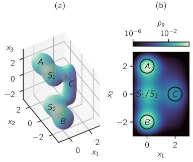

In our first example, we demonstrate the use of augmented TPT to resolve individual reaction steps. We consider a reaction through an intermediate with the three-dimensional potential
| (88) | ||||
where . We visualize the isosurface and the probability density on the CV space in Figure 3.
Our reaction of interest is described by the indicator function
| (89) |
where we have defined the reactant , product , and intermediate to be
| (90) | ||||
and . This reaction represents, for instance, a catalyzed reaction where a substrate internal coordinate (represented by ) and the interaction of the substrate with the catalyst (represented by ) can be observed while the status of the reaction (represented by ) cannot. The observable variables form the CV space , and the sets , , and are defined on this CV space.
There are two pathways in this reaction: uncatalyzed and catalyzed. In the uncatalyzed pathway, the system transitions from the reactant to , then crosses directly to before entering the product . In the catalyzed pathway, instead of directly crossing from to , the system transitions from into the intermediate and then to .
We select trajectories that react through each pathway by applying augmented TPT to the reaction. We define an augmented process for each of the pathways by including only the terms from (79) that are involved in that pathway. For the uncatalyzed pathway, we remove all reactive trajectories that visit the intermediate by removing all terms that contain from (79), yielding
| (91) |
and then select reactive trajectories using
| (92) |
For the catalyzed pathway, we retain only reactive trajectories that pass through the intermediate by removing all terms that contain as well as the direct transition from to , which does not pass through . This yields the augmented process
| (93) |
We then select reactive trajectories using
| (94) |
where . We show the possible transitions of (91) in Figure 4(a) and (93) in Figure 4(b).
Our goal is to visualize the mechanism of the reaction in the CV space and quantify the relative rates of the two pathways. To this end, we examine four reactive statistics: the reactive density , the reactive current , the forward committor , and the conditional mean first passage time to the product .
We plot the reactive statistics from traditional TPT in Figure 5(a). The reactive density reveals that reactive trajectories spend much of their time around and , which is consistent with the presence of intermediates / and . The reactive current (vector field) suggests that the reaction is dominated by the uncatalyzed pathway, although a significant fraction does react through the catalyzed pathway. The forward committor changes rapidly around , suggesting the presence of a bottleneck, corresponding to direct crossing from to . It is almost uniform around , suggesting the presence of the intermediate . The conditional mean first passage time can be interpreted in the same way as the forward committor; however, it allows us to visualize the order in which states are visited more clearly. The region below has a higher value of than the region around , which suggests that reactive trajectories usually visit the former before the latter. Together, these reactive statistics suggest a cohesive picture. The reaction is dominated by the uncatalyzed pathway, which has a bottleneck around . Reactive trajectories may leave this pathway before the bottleneck into the catalyzed pathway, which has an intermediate , and return after the bottleneck (i.e., they appear to circumvent /).
Some of the results from traditional TPT are misleading. For example, traditional TPT suggests that the uncatalyzed pathway is dominant, yet the total reactive flux from to is , while the reactive flux for trajectories that visit is , i.e., of trajectories go through the intermediate. This results from the restriction of the observed coordinates to ; in the full state space , traditional TPT is capable of correctly resolving the two pathways. However, we note that even given , traditional TPT cannot calculate dynamical statistics for the ensemble of trajectories that react through a particular pathway. Augmented TPT provides a solution to the overlap issue and enables the calculation of reactive statistics for individual steps of each pathway.
We first analyze the uncatalyzed pathway, which was wrongly suggested by traditional TPT to be the dominant pathway. Reactive statistics for this pathway are shown in Figure 5(b). As we would expect, the reactive density shows that reactive trajectories spend much of their time around /, and the reactive current suggests that reactive trajectories flow directly from to / to , without any notable deviation to the vicinity of . On the uncatalyzed pathway, the forward committor changes rapidly around due to the transition from to . Off the uncatalyzed pathway, the forward committor has a higher value closer to and a lower value closer to . This is surprising and results from slight differences in the reactive density at different values of . The conditional mean first passage time rapidly decreases near /, suggesting the same single bottleneck.
We now analyze the catalyzed pathway through the intermediate , which dominates the rate. We select trajectories that react through this pathway using (94). Augmented TPT enables us to split the pathway into individual steps, and so resolve the structure of each reaction step. The first step () starts when the reactive trajectory leaves the reactant and ends when it first enters the intermediate . The second step () starts at the first time the reactive trajectory enters , and ends at the last time the reactive trajectory leaves . The third step () starts when the reactive trajectory last leaves the intermediate and ends when it enters the product . As we now explain, separating the catalyzed pathway into these steps leads to reactive statistics that lead to a different interpretation than those from traditional TPT.
In the first step, the reactive density and reactive current clearly show that most reactive trajectories flow through an intermediate near , in this case , rather than a more direct path from to , as suggested by the reactive current from traditional TPT. Likewise, in the last step, they show that most reactive trajectories flow through an intermediate near , in this case . The absence of any significant reactive current in the second step, along with the high reactive density near , suggests that reactive trajectories predominantly remain in during this step, with a few trajectories transitioning back and forth to /, where there is a lower value of reactive density. The reactive current from traditional TPT is misleading because the flows from to and from to cancel each other, since and overlap in the CV space.
The forward committor on the catalyzed pathway is uniformly low in the first step and uniformly high in the third step. This suggests that the main bottleneck occurs in the second step, where around . The abrupt changes between steps suggest that the dynamics of the variables not captured within the CV space are influential in determining whether the reaction occurs. For the second step, we note that the low value of below and high value above reflect the full three-dimensional potential (Figure 3(a)). In traditional TPT, the high value of in the first step and the low value in the third step cancel, giving rise to the apparent rapid change near .
In the first step, decreases from to , suggesting the presence of a bottleneck between intermediates to . The same holds for the second step, suggesting that if the system crosses back to an intermediate near , it needs to overcome the same bottleneck to return to . In the third step, decreases from to , marking the transition from to . We note that this decrease occurs at a slightly lower value than in the uncatalyzed pathway. This separation of the two bottlenecks lies in contrast with from traditional TPT, where the superposition of the two bottlenecks creates an apparent bottleneck near , which conflates the dynamics of the catalyzed and uncatalyzed pathways.
Overall, we see that the statistics from traditional TPT qualitatively resemble a superposition of those for the uncatalyzed pathway and those associated with the second step of the catalyzed pathway, in which the system is mainly localized at . The important contributions from the first and third steps of the catalyzed pathway mask each other in traditional TPT.
VI.2 Reaction with Multiple Pathways
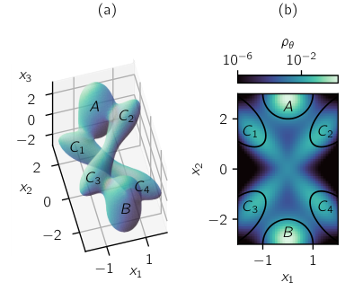

For our second example, we demonstrate the use of augmented TPT to separate pathways which overlap in the CV space. We consider overdamped Langevin dynamics on the three-dimensional potential
| (95) | ||||
where . As previously, these dynamics satisfy the Fokker–Planck equation in (87). The isosurface for this potential is shown in Figure 6(a), and the probability distribution on the coordinates, which we use as CVs, is shown in Figure 6(b). We define the reactant , product , and intermediates , , , and to be
| (96) | ||||
We also define the sets and . The reaction of interest is specified through the indicator function
| (97) |
We use the intermediates to define pathways. This is advantageous because it is not possible to divide the space into regions corresponding to different pathways owing to overlap. We define four pathways: major pathways I and II, and minor pathways III and IV. We define pathway I to first hit intermediate after leaving and last hit intermediate before hitting . We likewise define pathway II with , pathway III with , and pathway IV with .
To define means of selecting these pathways, we label a trajectory before the reaction with and after the reaction with . When the reaction is in process, we label times before the reactive trajectory first enters with , after the reactive trajectory last exits with , and between those times with . Then, we select pathways using
| (98) |
where . This choice of corresponds to
| (99) |
The first five terms of (99) denote the sets in which may be for each of the labels , and the remaining six terms describe the permitted transitions between the labels. We represent (99) visually in Figure 7. For instance, the seventh term, , corresponds to the single timestep transition from to and associates this with a change in the label from to .
We determine the reactive flux associated with each pathway and compare it with the total reactive flux. For the reaction specified by (97), the total reactive flux is . Each of the major pathways has a reactive flux of , which is of the total reactive flux. Each of the minor pathways has a reactive flux of , which is of the total reactive flux. These four pathways thus give rise to of the total reactive flux, and so are representative of the majority of reactive trajectories. The remaining 5% results from trajectories that do not conform to these pathways (e.g., ones that pass through only a single intermediate).
In Figure 8, we plot four reactive statistics: the reactive density , the reactive current , the conditional mean last passage time from the reactant , and the conditional mean first passage time to the product .
Reactive statistics from traditional TPT are shown in Figure 8(a). From the reactive density , we observe that reactive trajectories spend most of their time in the X-shaped region that connects the intermediates. The reactive current suggests that the majority of the reactive trajectories flow from the reactant to either or , then to either or via , and lastly to the product . Importantly, even if we consider the full state space , we cannot determine the relative weights of these four possible pathways, because the pathways are composed of segments that belong to multiple pathways (e.g., the first half of pathway III overlaps with pathway I and the second half of pathway III overlaps with pathway II) and the transitions through along pathways III and IV occur in opposite directions. Other quantities calculated using traditional TPT have the same issue. Both and are unable to distinguish between the pathways and only indicate the presence of a bottleneck between and .
In Figure 8(b), we visualize the reactive statistics for the major pathways. As pathway I and pathway II are mirror images of one another, we discuss only pathway I. The reactive current clearly shows that the system transitions directly between on-pathway intermediates, from to to to . The reactive density corroborates this picture, with relatively little density in and compared to and . We observe that and are highest near and , suggesting that these configurations are dynamically disconnected from the main flow of the reactive trajectories. The transition from to is accompanied by an abrupt increase in and an abrupt decrease in , which shows that a transition bottleneck is traversed. We note that the sharp increase in from to and the sharp decrease in from to imply the presence of bottlenecks between each of these pairs of states.
The minor pathways in Figure 8(c) result from trajectories that switch between the major pathways. Since the two minor pathways are mirror images of each other, we discuss only pathway III, which involves a switch from pathway I to pathway II. In contrast with the major pathways, the reactive density indicates that the system is likely to visit off-pathway intermediates and on its way from to . The conditional mean last passage time from the reactant is nearly identical to that of pathway I, with higher values near and and lower values near and . However, the conditional mean first passage time to the product is nearly identical to that of pathway II. In conjunction with , the slight increase in from to suggests that these intermediates readily interconvert, and similarly for the slight increase in from to . The larger change in and between and implies a bottleneck between and . This bottleneck is significant because the transition from to must occur for this pathway. As with the major pathways, there are also bottlenecks between and , and and .
VII Discussion
In this paper, we introduced an augmented process that labels sequences of events. This process enabled us to write statistics that depend on knowledge of past and future events in terms of quantities that are local in time and in turn to extend the TPT framework. We demonstrated how this framework can be used to separate statistics of competing pathways in reactions with intermediates to reveal features of mechanisms that are not apparent from traditional TPT analyses. Our framework can also be used to treat new classes of reactions that are not amenable to TPT analyses. For instance, reactions with the same reactant and product states, such as cycles of oscillators and excitable systems, can be handled using augmented TPT but not traditional TPT.
Our framework generalizes a previous extension of TPT Miron et al. 2021 and history augmented approaches for computing rates Suárez, Adelman, and Zuckerman 2016; Vanden-Eijnden and Venturoli 2009; Dickson, Warmflash, and Dinner 2009 and reactive statistics Vani, Weare, and Dinner 2022. The augmented process that we introduce is distinct from that in ref. Helfmann et al. 2020, in which the state space is expanded to include a time variable to treat time-dependent processes, including transient relaxations and systems with periodically varying dynamics. As a result, the two approaches can be combined to treat sequences of events of finite-time processes.
Our focus here was on establishing the conceptual framework for augmented TPT, and the examples that we showed were sufficiently simple that the Fokker–Planck equations defining their dynamics could be numerically integrated in the variables by quadrature. The dynamics of models with larger numbers of variables must instead be sampled through simulations that generate stochastic realizations of trajectories (i.e., the dynamics of the variables are numerically integrated in time). Because, like traditional TPT, the framework casts statistics in terms of quantities that are local in time, we can extend methods that compute reactive statistics from short trajectories Thiede et al. 2019; Strahan et al. 2021; Vani, Weare, and Dinner 2022. Such efforts are underway.
Acknowledgments
We acknowledge Adam Antoszewski, Spencer Guo, John Strahan, and Bodhi Vani for useful discussions. We thank the Research Computing Center at the University of Chicago for computational resources. This work was supported by National Institutes of Health award R35 GM136381 and National Science Foundation award DMS-2054306.
Appendix A Finite Difference Scheme
For a time-reversible drift-diffusion process
| (100) |
with stationary distribution , the infinitesimal generator can be used to compute expectations forward-in-time as
| (101) |
To evaluate expectations by quadrature, we adapt the finite difference scheme from ref. Thiede et al. 2019, which we reproduce here. We approximate (100) as a discrete time Markov jump process with time step on a grid with uniform spacing . For a small change in the direction of the th coordinate with magnitude , we substitute and then make the approximation
| (102) | ||||
Alternatively, we can write
| (103) | ||||
| (104) |
where represents the approximation of on the grid. Above, the first equality follows from the definition of conditional expectation, and the second assumes that all transitions within time are to neighboring grid points.
References
References
- Hänggi, Talkner, and Borkovec (1990) P. Hänggi, P. Talkner, and M. Borkovec, “Reaction-rate theory: fifty years after Kramers,” Rev. Mod. Phys. 62, 251–341 (1990).
- Peters (2017) B. Peters, Reaction Rate Theory and Rare Events (Elsevier, 2017).
- E and Vanden-Eijnden (2006) W. E and E. Vanden-Eijnden, “Towards a theory of transition paths,” J. Stat. Phys. 123, 503–523 (2006).
- Vanden-Eijnden (2006) E. Vanden-Eijnden, “Transition path theory,” in Computer Simulations in Condensed Matter Systems: From Materials to Chemical Biology Volume 1, Lecture Notes in Physics, edited by M. Ferrario, G. Ciccotti, and K. Binder (Springer, Berlin, Heidelberg, 2006) pp. 453–493.
- E and Vanden-Eijnden (2010) W. E and E. Vanden-Eijnden, “Transition-path theory and path-finding algorithms for the study of rare events,” Annu. Rev. Phys. Chem. 61, 391–420 (2010).
- Metzner, Schütte, and Vanden-Eijnden (2009) P. Metzner, C. Schütte, and E. Vanden-Eijnden, “Transition path theory for markov jump processes,” Multiscale Model. Simul. 7, 1192–1219 (2009).
- Metzner, Schütte, and Vanden-Eijnden (2006) P. Metzner, C. Schütte, and E. Vanden-Eijnden, “Illustration of transition path theory on a collection of simple examples,” J. Chem. Phys. 125, 084110 (2006).
- Du et al. (1998) R. Du, V. S. Pande, A. Y. Grosberg, T. Tanaka, and E. S. Shakhnovich, “On the transition coordinate for protein folding,” J. Chem. Phys. 108, 334–350 (1998).
- Suárez, Adelman, and Zuckerman (2016) E. Suárez, J. L. Adelman, and D. M. Zuckerman, “Accurate estimation of protein folding and unfolding times: beyond Markov state models,” J. Chem. Theory Comput. 12, 3473–3481 (2016).
- Vanden-Eijnden and Venturoli (2009) E. Vanden-Eijnden and M. Venturoli, “Exact rate calculations by trajectory parallelization and tilting,” J. Chem. Phys. 131, 044120 (2009).
- Dickson, Warmflash, and Dinner (2009) A. Dickson, A. Warmflash, and A. R. Dinner, “Separating forward and backward pathways in nonequilibrium umbrella sampling,” J. Chem. Phys. 131, 154104 (2009).
- Vani, Weare, and Dinner (2022) B. P. Vani, J. Weare, and A. R. Dinner, “Computing transition path theory quantities with trajectory stratification,” J. Chem. Phys. 157, 034106 (2022).
- Miron et al. (2021) P. Miron, F. J. Beron-Vera, L. Helfmann, and P. Koltai, “Transition paths of marine debris and the stability of the garbage patches,” Chaos 31, 033101 (2021).
- Helfmann et al. (2020) L. Helfmann, E. Ribera Borrell, C. Schütte, and P. Koltai, “Extending transition path theory: periodically driven and finite-time dynamics,” J. Nonlinear Sci. 30, 3321–3366 (2020).
- Finkel et al. (2021) J. Finkel, R. J. Webber, E. P. Gerber, D. S. Abbot, and J. Weare, “Learning forecasts of rare stratospheric transitions from short simulations,” Monthly Weather Review 149, 3647–3669 (2021).
- Thiede et al. (2019) E. H. Thiede, D. Giannakis, A. R. Dinner, and J. Weare, “Galerkin approximation of dynamical quantities using trajectory data,” J. Chem. Phys. 150, 244111 (2019).
- Strahan et al. (2021) J. Strahan, A. Antoszewski, C. Lorpaiboon, B. P. Vani, J. Weare, and A. R. Dinner, “Long-time-scale predictions from short-trajectory data: a benchmark analysis of the trp-cage miniprotein,” J. Chem. Theory Comput. 17, 2948–2963 (2021).