Multi-fidelity uncertainty quantification of particle deposition in turbulent pipe flowJournal: Journal of Aerosol Science

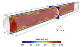
The problem under consideration consists of a cylindrical pipe with diameter $D=20$ mm (see Fig. 2). The length of the pipe is $L=10D$ to ensure domain independent results. The pipe is periodic in the streamwise ($x$) direction. The fluid is taken to be air with kinetic viscosity $\nu=1.5\times 10^{-5}$ and bulk velocity $U_{b}=4.0$ m/s, corresponding to a Reynolds number based on the friction velocity of $\rm{Re}_{\tau}=180$ and a Reynolds number based on the bulk velocity $\rm{Re}=5333$. Monodisperse spherical particles of three different diameters $d_{p}=1.6$ $\upmu$m, $5$ $\upmu$m and $16$ $\upmu$m and density $\rho_{p}=2650$ kg/m³ are considered. The simulations consist of $N=10^{6}$ particles to ensure a statistically significant sample size, corresponding to an average number density $n_{p}=1.6\times 10^{10}$ m^-3. Particles are randomly distributed within the domain and reach a statistically stationary state where the particle mass flux at the wall is constant in the radial direction. Particle inertia is characterized by a non-dimensional particle response time $\tau_{p}^{+}=\tau_{p}/\tau_{f}$, where $\tau_{p}=\rho_{p}d_{p}^{2}/(18\rho\nu)$ is the particle response time and $\tau_{f}=\nu/u_{*}^{2}$ is the frictional time scale. The three particle sizes considered correspond to $\tau_{p}^{+}=0.1,1,{\rm and\ }10$.

To investigate the effect of charge on particle dynamics and deposition, each particle is assigned a unique value $q_{p}$ that is proportional to the maximum possible charge $q_{\rm max}$ according to $q_{p}=\xi q_{\rm max}$, with $0\leq\xi\leq 0.1$. The maximum charge is given by [97]

In this study, we consider $\xi=0$ (no charge) and $\xi=0.1$, representative of typical values for charge measured in dustry turbulent pipe flows [98, 99, 100]. The Hamaker constant, $A$, is varied between $10^{-20}\,$J for weakly cohesive particles (e.g., silica) to $10^{-18}\,$J for strongly cohesive materials such as metal oxides [101]. Similarly, a non-dimensional parameter $\zeta=A/A_{0}$ is introduced with $A_{0}=10^{-18}\,$J. We consider $0\leq\zeta\leq 1$.

The deposition rate is typically characterized using the non-dimensional deposition velocity [28, 102, 103, 40, 104, 39], given by

where $J_{w}$ is the particle mass flux to the wall per unit area, $\rho_{pm}$ is the mean particle bulk density in the pipe and $u_{*}=\sqrt{\tau_{w}/\rho}$ is the friction velocity with $\tau_{w}$ the wall shear stress. Throughout the rest of this paper, $\zeta$ and $\xi$ are taken as input parameters that introduce parametric uncertainty to the system, and $V_{\rm dep}^{+}$ is the system output or QoI. Thus, we will perform UQ and GSA targeting the QoI $V_{\rm dep}^{+}$.

Before performing UQ and GSA, we first analyze the order of magnitude in van der Waals and electrostatic forces in wall-bounded systems with different particle loadings. The magnitude of the van der Waals force between two particles $i$ and $j$ of the same size is given by

where $\delta_{ij}$ is the distance between the particle surfaces, and $A$ is the Hamaker constant. Due to its short range nature, it is assumed that the force saturates at a minimum separation, $\delta_{\text{min}}=1\times 10^{-9}$ m and is cut off at $\delta_{\text{max}}=d_{p}/4$. The magnitude of the electrostatic force is given by Coulomb’s law according to

where $q_{p}^{(i)}$ and $q_{p}^{(j)}$ are the charges belonging to particles $i$ and $j$, respectively, and $\epsilon_{0}=8.854\times 10^{-12}$ $\text{F}\cdot\text{m}^{-1}$ is the vacuum permittivity. Details on the numerical discretization of these forces can be found in A.

Figure 3a shows the particle acceleration due to these two forces ($\xi=0.1$ and $\zeta=1$) as a function of particle separation distance via a direct evaluation of Eqs. (3) and (4). The van der Waals force is seen to be the dominant mode of deposition at short separation ($\delta_{12}<\mathcal{O}(10^{-6}\,{\rm m})$), but is surpassed by electrostatic forces at longer range. The influence of the van der Waals force decays with increasing particle size, whereas the electrostatic force results in higher particle acceleration for larger particles at long distances.

From Fig. 3a, the average particle acceleration can be estimated for a given number density $n_{p}$. By assuming a random distribution of particles, the average distance between particles $\delta_{12}=n_{p}^{-1/3}$. Let $F_{12}(\delta_{12})$ denote the force between two particles given by Eqs. (3) and (4) as a function of separation distance. The domain-averaged particle-particle force is therefore $\overline{F}_{12}=F_{12}(1/{n_{p}}^{1/3})$. The particle-wall force $F_{\rm wall}(\delta_{12})=2F_{12}(\delta_{12})$ for van der Waals interactions and $F_{\rm wall}(\delta_{12})=F_{12}(2\,\delta_{12})$ for electrostatic interactions, where image charging is assumed by placing an image particle of opposite charge mirrored at the same distance across the wall. The domain-averaged particle-wall force is estimated by integrating the force in the radial direction

where $r_{\rm cutoff}=\delta_{\min}$ for van der Waals and $r_{\rm cutoff}=d_{p}/2$ for electrostatics to avoid singularity. The accelerations due to estimated forces are compared in Fig. 3b. It can be seen that domain-averaged particle-particle contributions increase with $n_{p}$ while particle-wall contributions are insensitive to the particle loading. As a result, the relative importance of these four different forces strongly depends on $n_{p}$. For instance, the particle-particle electrostatic force surpasses particle-wall image charging when $n_{p}\gtrsim\mathcal{O}(10^{11})$. Due to the short-range nature of van der Waals interactions, however, the particle-wall contribution is always greater than the inter-particle van der Waals attraction. For the system considered herein ($n_{p}=1.6\times 10^{10}$), the relative importance is ranked as particle-wall electrostatics, particle-particle electrostatics, particle-wall van der Waals, and particle-particle van der Waals, which is orders of magnitudes smaller than the former three.

The non-dimensional deposition velocity predicted by the one-dimensional Eulerian model of Guha 2008 is shown in Fig 4. For the range of parameters considered, the electrostatic force is seen to have a larger effect on the deposition rate than the van der Waals force across all particles sizes, which is consistent with the direct evaluation of Eqs. (3) and (4) reported in Fig. 3b. In addition, the electrostatic force exhibits the largest enhancement in deposition for mid-sized particles (diffusion-impaction regime), for which the charge amount is significant and at the same time particles are most responsive to the turbulent eddies. Van der Waals interactions, on the other hand, primarily affect the deposition rate of small particles (turbulent diffusion regime).

In this work, two model fidelities are considered to facilitate UQ and GSA in the later sections. The high-fidelity model is taken to be a direct numerical simulation (DNS) of the fully-developed turbulent pipe flow presented in § 2.1. The one-dimensional Eulerian model proposed by Guha 2008 is used for the low-fidelity model. Details of each model are described in A and B. In this section, the relative importance of cohesive forces on particle deposition is quantified, and a comparison is made between the high- and low-fidelity models. Multi-fidelity UQ is then presented in the following section.

The efficacy of MFMC for UQ of particle deposition depends on how strongly the two models correlate (as long as the low-fidelity prediction varies in a correlated manner to its high-fidelity counterpart—not necessarily needing to be accurate—then it could be made into a good predictor to the high-fidelity behavior). To illustrate the correlation between the models and also to gain an initial physical intuition for the problem, in this section we evaluate a set of high-fidelity (DNS) and low-fidelity (Eulerian one-dimensional model) simulations systematically in the parameter space ($\xi$ and $\zeta$). In particular, we endow uniform uncertainty distributions for both $\xi$ and $\zeta$ across their allowable ranges ($\xi\in[0,0.1]$, $\zeta\in[0,1]$), representing a scenario where all values within their ranges are equally likely to occur. The uniform distribution appeals to the principle of maximum entropy [105] that makes the fewest assumption in distribution formation when upper and lower bounds are given. 100 simulations are then performed for both models by uniformly probing the parameter space shown in Fig. 5. We emphasize that this is not part of the MFMC or MC sampling, but rather a “brute-force” illustration using a tensorized sweep of the entire parameter space, which is achievable here because the parameter space is only two-dimensional.

Three particle sizes ($\tau_{p}^{+}=0.1,1,{\rm and\ }10$) are considered, corresponding to each deposition regime. The deposition rates obtained using DNS are measured from the rates at which the number of deposited particles $N_{\rm dep}$ increases in time. As shown in Figs. 6a–6c, $N_{\rm dep}$ grows linearly in time after a short initial transient ($t/\tau_{f}<10$), beyond which the deposition rate can be uniquely determined. The van der Waals interaction is seen to have comparable effects on the deposition rate to the electrostatic force for small particles ($\tau_{p}^{+}=0.1$), resulting in a wide spread of the deposition curves. However, as the electrostatic contribution quickly surpasses the van der Waals for larger particles, the variation in van der Waals strength ($\zeta$) exhibits little effect on the deposition except when $\xi\approx 0$.

The computed deposition rate in terms of non-dimensional deposition velocity $V_{\rm dep}^{+}$ is compared with the one-dimensional Eulerian model predictions in Figs. 6d–6f. The one-dimensional model is seen to under-predict $V_{\rm dep}^{+}$ for all three particle sizes, especially for mid-size particles for which clustering due to turbulence is expected to be most significant. Recall that the one-dimensional model only accounts for particle-wall interactions and the particle distribution is assumed to be only a function of wall distance. Thus, spatial inhomogeneities due to preferential concentration and low-speed streak regions along the wall are neglected. These inhomogeneities amplify particle-particle interactions and collision rates, which may potentially contribute to particle deposition. Nevertheless, the general trends of $V_{\rm dep}^{+}$ predicted by the one-dimensional model and three-dimensional DNS are in reasonable agreement. The high correlation between the two models suggests that MFMC UQ, presented in the following section, will likely provide substantial benefits.

The high-fidelity model (DNS) is denoted as

where $\bm{x}\in\mathcal{X}$ is the input and $y=f^{(1)}(\bm{x})\in\mathcal{Y}$ is the output. Here, the input parameters $\xi\in[0,\,0.1]$ and $\zeta\in[0,\,1]$ together form a random vector $\bm{X}$ associated with a probability distribution, which in this case is the uniform distribution discussed earlier. The output $Y=V_{\rm dep}^{+}=f^{(1)}(\bm{X})$ is therefore a random variable whose distribution is induced by the distribution of $\bm{X}$. Our goal is to characterize the distribution of $f^{(1)}(\bm{X})$, or more precisely, find the pushforward probability measure for $\bm{X}$ through the mapping $f^{(1)}$.

Typically, we are interested in expectations of various functions with respect to this distribution (e.g., $\mathbb{E}[h(Y)]$), which can be estimated using MC. For clarity, we present MC below in terms of the expected value $\mathbb{E}[Y]$ (i.e. the mean), but the results are valid for general expectations with $h(Y)$ as well. The MC estimator for

is

where $\bm{x}_{j}$ are independent and identically distributed (i.i.d.) samples of $\bm{X}$. The MC estimator is unbiased ($\mathbb{E}\left[\overline{y}_{m}\right]=S$), and so its mean-squared error (MSE) also equals to the estimator variance

Under the reasonable assumption that the computational cost of each high-fidelity model run is approximately the same, the total computational cost of the MC estimator $\overline{y}_{m}$ is then

where $w$ is the unit cost of each high-fidelity evaluation. Depending on the variance of the output variable ($\operatorname{Var}[f^{(1)}(\bm{X})]$), a large number of high-fidelity model evaluations ($m$) may be necessary to obtain an MC estimate with an acceptable MSE. If the high-fidelity model is expensive to evaluate, then MC estimation can become intractable.

MFMC makes use of low-fidelity models, in addition to the high-fidelity model, with the aim to minimize the MC estimator MSE by optimizing the number of evaluations for each model under a given total computational budget. Suppose we have $k$ models sorted in descending fidelity $f^{(1)},\ldots,f^{(k)}$ ($f^{(1)}$ is still our targeted high-fidelity model), each evaluated $m_{k}$ times ($0<m_{1}\leq m_{2}\leq\cdots\leq m_{k}$), then their individual MC estimators are defined by

The MFMC estimator for the highest fidelity model is formed using the control variates technique, through a linear combination of these MC estimators:

MFMC seeks the set of coefficients $\alpha_{i}$ and number of evaluations $m_{i}$ that minimizes $\operatorname{Var}[\hat{S}]$ subject to the total cost constraint

where $w_{i}$ is the unit cost of model $f^{(i)}$ and $p$ is the given total computational budget. The optimization procedure requires the correlation coefficients between each low-fidelity model to the targeted high-fidelity model, given by

An analytical solution [84] to this optimization problem yields, for $i=2,\ldots,k$:

where $m_{1}^{*}=p/(\bm{w}^{T}\bm{r}^{*})$ and $\sigma_{i}=\sqrt{\operatorname{Var}\left[f^{(i)}(\bm{X})\right]}$ is the standard deviation of model $f^{(i)}(\bm{X})$. A mild condition on the model costs is required for this analytical solution to exist:

for $i=2,\ldots,k$ with $\rho_{1,k+1}=1$. We will show in § 4.1 that Eq. (18) can be easily satisfied for our purposes.

Variance-based GSA provides a quantitative measure of how uncertainty from each model input contributes to the overall uncertainty in the model output QoI, through the Sobol’ indices. The two most commonly used Sobol’ indices are the main-effect index and total-effect index. The main-effect index measures variance contribution solely due to the $j$-th input:

where $Y$ is the output QoI and $\bm{X}_{\sim j}$ denotes the set of all input variables except the $\bm{X}_{j}$ component. The total-effect index measures variance contributions from all terms that involve the $j$-th parameter, including higher-order interaction effects among multiple inputs that involve the $j$-th parameter:

Thus, the difference between $s_{j}$ and $s_{j}^{t}$ offers a sense about the presence of interaction effects without explicitly computing them.

While these Sobol’ indices can be estimated with single-fidelity MC sampling [91, 92, 93, 94], Qian et al. 2018 has recently proposed a MFMC estimator similar to the form of Eq. (12). The MFMC estimate of the Sobol’ indices are $s_{j}=\hat{V}_{j,\mathrm{mf}}/{{\rm Var}(Y)}$ and $s_{j}^{t}=\hat{T}_{j,\mathrm{mf}}/{{\rm Var}(Y)}$, where

and

We further adopt an unbiased MC estimator for $\hat{V}_{j,m_{i}}^{(i)}$ and $\hat{T}_{j,m_{i}}^{(i)}$ proposed by Owen 2013:

and

where $\mbox{\boldmath{$z$}}_{i}^{(j)}=(\mbox{\boldmath{$x$}}_{i}^{\prime}(1),\dots,\mbox{\boldmath{$x$}}_{i}^{\prime}(j-1)),\mbox{\boldmath{$x$}}_{i}(j),\mbox{\boldmath{$x$}}_{i}^{\prime}(j+1),\dots,\mbox{\boldmath{$x$}}_{i}^{\prime}(d))$ with $d$ being the number of input parameters, $\hat{E}$, $\hat{E}^{\prime}$ and $\hat{V}$, $\hat{V}^{\prime}$ are the sample means and variances estimated using two sets of $m_{i}$ independent realizations of input $\bm{X}$ respectively ($\bm{x}_{1},\ldots,\bm{x}_{m_{i}}$ and $\bm{x}^{\prime}_{1},\ldots,\bm{x}^{\prime}_{m_{i}}$). Furthermore, Qian et al. 2018 demonstrated that the same optimization procedures (Eqs. (15)–(17)), namely same $\alpha_{i}$ and $m_{i}$ for $i=2,\dots,k$, can be used for the MFMC estimates of the Sobol’ indices without sacrificing the performance of the algorithm.

Prior to preforming the actual uncertainty quantification, it is important to ensure the MFMC precondition (Eq. (18)) is met and the MFMC estimator is superior to the classic MC estimator for the two models considered in this study. To assess the performance of an estimator, the MSE introduced in Eq. (9) is typically used and estimated using samples:

where $S_{i}=f^{(i)}(\mbox{\boldmath{$x$}})$ and $\hat{S}$ is the estimator prediction. In the case of two models, Peherstorfer et al. 2016 derived an analytical estimate of the variance reduction achieved by the MFMC estimator compared to the classic MC estimator given as

where $\gamma$ is the variance reduction ratio, $\hat{S}_{\rm mf}$ denotes the MFMC estimator.

Figure 7 shows the contour plot of $\gamma$ for $\rho_{12}\in[0,1]$ and $w_{2}/w_{1}\in[10^{-5},10^{-1}]$. The multi-fidelity approach fails when $\gamma>1$ or the precondition (Eq. (18)) is not met. However, this only occurs for extreme cases, either highly uncorrelated models (e.g., $\rho_{12}<0.3$) or expensive low-order models (e.g., $w_{2}/w_{1}>10^{-2}$). The values in Table 2 yield $\gamma=0.028,0.014,$ and 0.135 for $\tau_{p}^{+}=0.1,1,$ and 10 respectively, confirming that the MFMC estimator will significantly improve MSE using these two models.

Using the prior estimates of the model statistics provided in Table 2, the effective budget $p_{\rm eff}$ is then distributed among our two models of consideration. Table 3 summarizes the number of evaluations, $m_{k}$, and the control variate coefficients $\alpha_{k}$ assigned by the MFMC approach for $p=36$ and $72$. The same set of $m_{k}$ and $\alpha_{k}$ is then used to estimate the mean, variance, and sensitivity indices. As expected, more evaluations are performed for the one-dimensional model when it is more correlated with the DNS predictions (e.g., $\tau_{p}^{+}=1$), and a higher coefficient $\alpha_{k}$ is required when the one-dimensional model under-predicts $\sigma_{k}$ (e.g., $\tau_{p}^{+}=1$ and $10$). The classic MC method using only high-fidelity (DNS) and only low-fidelity (one-dimensional Eulerian) models are also included for subsequent comparisons.

Figure 8 quantifies the uncertainty in mean and standard deviation of $V_{\rm dep}^{+}$ predicted by MC estimators (using only DNS or one-dimensional models) and MFMC with the same budget $p=72$. Statistics of 100 estimate replicates are shown as box plots in which the central mark indicates the median, and the bottom and top edges of the box mark the 25-th and 75-th percentiles, respectively. The whiskers extend to the lower and upper bounds of the dataset. The MFMC estimators admit notably lower variance in both the predicted mean and standard deviation compared to the high-fidelity MC estimators. Although the variance predicted by low-fidelity MC estimator is the smallest due to a larger number of evaluations, it suffers inevitable bias due to its modeling error (with respect to the high-fidelity model) and therefore deviates from the “true” solutions, which are taken from well-converged MC estimates using $p=50000$ by randomly sampling from the 100 pre-computed DNS cases.

The distribution of mean and standard deviation estimates from 100 replicates of MFMC and MC estimators are shown in Fig. 9 for $p=72$ and $\tau_{p}^{+}=0.1$ as an example. The variations in both mean and standard deviation are significantly reduced using MFMC as indicated by the narrower distributions. The distributions are not noticeably skewed which makes the standard deviation a sufficient statistical metric. Similar reduction in estimator variations is observed for other particle sizes and computational budgets considered in Fig. 8. Note that the MFMC estimators remain unbiased even though the low-fidelity model produces entirely different expected values compared to the high-fidelity model.

Figure 10 presents the estimated global sensitivity of $V_{\rm dep}^{+}$ using MC with only DNS (high-fidelity model) and MFMC. Data statistics of 100 estimate replicates are shown as box plots. Similar to the mean and standard deviation, the MFMC estimators admit smaller variance in the predicted Sobol’ indices compared to the classic MC estimators, allowing definitive ranking of input parameters (i.e., $\zeta$ and $\xi$) with $p=36$ while MC barely achieves this at $p=72$. For instance, the variation in MFMC’s $s_{m}^{1}$ with $p=36$ is smaller than MC’s $s_{m}^{1}$ obtained with a higher budget $p=72$ across all three particle sizes.

To more quantitatively assess the benefit of MFMC, estimated MSE is plotted in Fig. 11 for the MFMC estimator, MC estimator with only DNS, and MC estimator with only one-dimensional model. MSE is computed via Eq. (25) with $\hat{S}$ taken from a well-converged estimates using $p=50,000$ by randomly sampling from 100 DNS data. The MFMC estimator with $p=36$ achieves the same level of MSE compared to the classic MC estimator using only DNS data with $p=288$, which translates to at least 8 times speedup. Such cost saving is seen for estimation of all three quantities: mean, standard deviation, and Sobol’ index of $V_{\rm dep}^{+}$. Note that although using the low-fidelity model alone to estimate sensitivities exhibit small variation when the budget is small, it converges to a wrong solution as shown in Fig. 11b and 11c due to the bias from its modeling error. The bias in one-dimensional model prediction is also seen in Fig. 11a where the error in predicted mean of $V_{\rm dep}^{+}$ is orders of magnitudes larger than MFMC.

Finally, the predicted statistics of $V_{\rm dep}^{+}$ using MFMC with $p=288$ are tabulated in Table 4. Regarding uncertainty, the deposition rate of middle-sized particles ($\tau_{p}^{+}=1$ or $d_{p}=5\,\upmu$m) exhibits the largest standard deviation given the same variations in electrical charge and Hamaker constant, which is primarily due to these particles being most responsive to the turbulent eddies. Regarding sensitivity, van der Waals force has almost negligible effect on the deposition rates ($s_{m}^{1}\approx 0$) for $\tau_{p}^{+}=1$ and 10, but plays a bigger role for the smallest particles ($\tau_{p}^{+}=1$ or $d_{p}=1.6\,\upmu$m).

The demonstration thus far has been focusing on particle deposition under an all-stick assumption. However, both cohesion strength and temperature are known to affect the rebound mechanism of particles. To capture these effects, a physics-based model for temperature-dependent particle rebound is used [6], which incorporates material property sensitivity including yield stress $\sigma_{y}$ and normal coefficient of restitution ${\rm CoR}_{n}$ to temperature $T$ and normal impact velocity $V_{n1}$ observed in experiments. The model derives ${\rm CoR}_{n}$ based on energy conservation, which is given as

where $\sigma_{y}(T)=200-0.225(T-1000)$ MPa, $\gamma_{c}=A/(24\pi\delta_{c}^{2})$ is the cohesion potential energy with $\delta_{c}=0.165\,$nm, $A_{\rm cont}$ is the contact area between particle and wall, $E=70$ GPa is the Young’s modulus of particle. Similar to $\xi$ and $\zeta$, another input parameter $\theta=0.225(T-1000)/200\in[0,\,1]$ is introduced such that the $\sigma_{y}$ varies from 0 to $\sigma_{y}^{0}=200$ MPa, the particle yield stress under typical conditions.

Figure 12 shows how ${\rm CoR}_{n}$ depends on $\zeta$ and $\theta$ as a function of normal impact velocity $V_{n1}$ using the rebound model of Bons et al. 2017. It is observed that with increasing cohesion strength $\zeta$ or temperature $\theta$, ${\rm CoR}_{n}$ decreases for all impact velocities, indicative of more deposition. Here ${\rm CoR}_{n}=0$ represents that the particle is deposited and all-stick condition applies.

Using MFMC together with the deposition model of Bons et al. 2017, we can eliminate the all-stick constraint. However, since particle rebound is not accounted in the definition of $V_{\rm dep}^{+}$, a new QoI known as capture efficiency (CE) is introduced instead. CE is defined as the rate of deposited mass $\dot{m}_{\rm dep}$ over the total mass flow rate $\dot{m}_{\rm tot}$ given by

where $V_{\rm dep}^{+}|_{\rm stick}$ is the nondimensional deposition velocity of particles that do not rebound (${\rm CoR}_{n}=0$), the equality is achieved only when all-stick condition holds. CE incorporates the effect of particle rebound and is readily measurable in experiments [6, 31].

The main-effect Sobol’ indices of deposition, quantified by $V_{\rm dep}^{+}$ and ${\rm CE}$, due to variations in $\xi$, $\zeta$, and $\theta$ is shown in Fig. 13. It can be seen that after including the rebound physics, small particles become even more sensitive to van der Waals since adhesion reduces ${\rm CoR}_{n}$ and therefore prevents particles from rebound. In addition, large particles are more sensitive to temperature namely due to the decreased yield stress. This is because large particles impact the wall with higher impact velocities, which results in more plastic deformation especially at high temperatures. Nevertheless, the deposition process is still most sensitive to the variation in electrostatics. Finally, we note that although the scope of this paper is limited to particle deposition as a function of three input parameters, the same MFMC framework can be applied to study other multiphase flow problems and additional input parameters can be introduced at affordable computational costs.

References

- Begat et al. [2004] P. Begat, D. A. V. Morton, J. N. Staniforth, R. Price, The cohesive-adhesive balances in dry powder inhaler formulations II: influence on fine particle delivery characteristics, Pharmaceutical Research 21 (2004) 1826–1833.
- Yang et al. [2013] J. Yang, C.-Y. Wu, M. Adams, Dem analysis of particle adhesion during powder mixing for dry powder inhaler formulation development, Granular Matter 15 (2013) 417–426.
- Yang et al. [2015] J. Yang, C.-Y. Wu, M. Adams, Numerical modelling of agglomeration and deagglomeration in dry powder inhalers: a review, Current Pharmaceutical Design 21 (2015) 5915–5922.
- Batcho et al. [1987] P. F. Batcho, J. C. Moller, C. Padova, M. G. Dunn, Interpretation of gas turbine response due to dust ingestion, Journal of Engineering for Gas Turbines and Power 109 (1987) 344–352.
- Dunn et al. [1996] M. G. Dunn, A. J. Baran, J. Miatech, Operation of gas turbine engines in volcanic ash clouds, Journal of Engineering for Gas Turbines and Power 118 (1996) 724–731.
- Bons et al. [2017] J. P. Bons, R. Prenter, S. Whitaker, A simple physics-based model for particle rebound and deposition in turbomachinery, Journal of Turbomachinery 139 (2017) 081009.
- Sacco et al. [2018] C. Sacco, C. Bowen, R. Lundgreen, J. Bons, E. Ruggiero, J. Allen, J. Bailey, Dynamic similarity in turbine deposition testing and the role of pressure, Journal of Engineering for Gas Turbines and Power 140 (2018) 102605.
- Mikami et al. [1998] T. Mikami, H. Kamiya, M. Horio, Numerical simulation of cohesive powder behavior in a fluidized bed, Chemical Engineering Science 53 (1998) 1927–1940.
- van der Hoef et al. [2008] M. A. van der Hoef, M. van Sint Annaland, N. G. Deen, J. Kuipers, Numerical simulation of dense gas-solid fluidized beds: a multiscale modeling strategy, Annual Review of Fluid Mechanics 40 (2008) 47–70.
- Mahecha-Botero et al. [2009] A. Mahecha-Botero, J. R. Grace, S. Elnashaie, C. J. Lim, Advances in modeling of fluidized-bed catalytic reactors: a comprehensive review, Chemical Engineering Communications 196 (2009) 1375–1405.
- Pan et al. [2016] H. Pan, X.-Z. Chen, X.-F. Liang, L.-T. Zhu, Z.-H. Luo, CFD simulations of gas–liquid–solid flow in fluidized bed reactors—a review, Powder Technology 299 (2016) 235–258.
- Lai and Nazaroff [2000] A. C. Lai, W. W. Nazaroff, Modeling indoor particle deposition from turbulent flow onto smooth surfaces, Journal of Aerosol Science 31 (2000) 463–476.
- Lai [2002] A. Lai, Particle deposition indoors: a review, Indoor Air 12 (2002) 211–214.
- Geldart [1973] D. Geldart, Types of gas fluidization, Powder Technology 7 (1973) 285–292.
- Liu and Agarwal [1974] B. Y. Liu, J. K. Agarwal, Experimental observation of aerosol deposition in turbulent flow, Journal of Aerosol Science 5 (1974) 145–155.
- Friedlander and Johnstone [1957] S. Friedlander, H. Johnstone, Deposition of suspended particles from turbulent gas streams, Industrial & Engineering Chemistry 49 (1957) 1151–1156.
- Schwendiman and Postma [1962] L. Schwendiman, A. Postma, Turbulent deposition in sampling lines, Rapport technique Tech. Inf. Div. TID-7628, USAEC 118 (1962).
- Wells and Chamberlain [1967] A. Wells, A. Chamberlain, Transport of small particles to vertical surfaces, British Journal of Applied Physics 18 (1967) 1793.
- Sehmel [1968] G. A. Sehmel, Aerosol Deposition from Turbulent Airstreams in Vertical Conduits., Technical Report, Battelle-Northwest, Richland, Wash. Pacific Northwest Lab., 1968.
- Young and Leeming [1997] J. Young, A. Leeming, A theory of particle deposition in turbulent pipe flow, Journal of Fluid Mechanics 340 (1997) 129–159.
- Davies [1966] C. Davies, Deposition of aerosols from turbulent flow through pipes, Proceedings of the Royal Society of London. Series A. Mathematical and Physical Sciences 289 (1966) 235–246.
- Beal [1970] S. K. Beal, Deposition of particles in turbulent flow on channel or pipe walls, Nuclear Science and Engineering 40 (1970) 1–11.
- Wood [1981] N. Wood, A simple method for the calculation of turbulent deposition to smooth and rough surfaces, Journal of Aerosol Science 12 (1981) 275–290.
- Papavergos and Hedley [1984] P. Papavergos, A. Hedley, Particle deposition behaviour from turbulent flows, Chemical Engineering Research & Design 62 (1984) 275–295.
- Ounis et al. [1993] H. Ounis, G. Ahmadi, J. B. McLaughlin, Brownian particle deposition in a directly simulated turbulent channel flow, Physics of Fluids A: Fluid Dynamics 5 (1993) 1427–1432.
- Brooke et al. [1994] J. W. Brooke, T. Hanratty, J. McLaughlin, Free-flight mixing and deposition of aerosols, Physics of Fluids 6 (1994) 3404–3415.
- Wang and Squires [1996] Q. Wang, K. D. Squires, Large eddy simulation of particle-laden turbulent channel flow, Physics of Fluids 8 (1996) 1207–1223.
- Kallio and Reeks [1989] G. Kallio, M. Reeks, A numerical simulation of particle deposition in turbulent boundary layers, International Journal of Multiphase Flow 15 (1989) 433–446.
- Gosman and Loannides [1983] A. Gosman, E. Loannides, Aspects of computer simulation of liquid-fueled combustors, Journal of Energy 7 (1983) 482–490.
- Dehbi [2008] A. Dehbi, Turbulent particle dispersion in arbitrary wall-bounded geometries: A coupled CFD-Langevin-equation based approach, International Journal of Multiphase Flow 34 (2008) 819–828.
- Gnanaselvam et al. [2021] P. Gnanaselvam, C. H. Lo, J. Han, J. P. Bons, Turbulent dispersion and deposition of micron-sized particles in a turbulent pipe flow at high temperatures, in: AIAA Scitech 2021 Forum, 2021, p. 0850.
- Johansen [1991] S. Johansen, The deposition of particles on vertical walls, International Journal of Multiphase Flow 17 (1991) 355–376.
- Guha [1997] A. Guha, A unified Eulerian theory of turbulent deposition to smooth and rough surfaces, Journal of Aerosol Science 28 (1997) 1517–1537.
- Guha [2008] A. Guha, Transport and deposition of particles in turbulent and laminar flow, Annual Review of Fluid Mechanics 40 (2008) 311–341.
- Di Renzo and Urzay [2018] M. Di Renzo, J. Urzay, Aerodynamic generation of electric fields in turbulence laden with charged inertial particles, Nature Communications 9 (2018) 1676.
- Di Renzo et al. [2019] M. Di Renzo, P. Johnson, M. Bassenne, L. Villafañe, J. Urzay, Mitigation of turbophoresis in particle-laden turbulent channel flows by using incident electric fields, Physical Review Fluids 4 (2019) 124303.
- Karnik and Shrimpton [2012] A. U. Karnik, J. S. Shrimpton, Mitigation of preferential concentration of small inertial particles in stationary isotropic turbulence using electrical and gravitational body forces, Physics of Fluids 24 (2012) 073301.
- van Haarlem et al. [1998] B. van Haarlem, B. J. Boersma, F. T. Nieuwstadt, Direct numerical simulation of particle deposition onto a free-slip and no-slip surface, Physics of Fluids 10 (1998) 2608–2620.
- Zonta et al. [2013] F. Zonta, C. Marchioli, A. Soldati, Particle and droplet deposition in turbulent swirled pipe flow, International Journal of Multiphase Flow 56 (2013) 172–183.
- Marchioli et al. [2003] C. Marchioli, A. Giusti, M. V. Salvetti, A. Soldati, Direct numerical simulation of particle wall transfer and deposition in upward turbulent pipe flow, International Journal of Multiphase Flow 29 (2003) 1017–1038.
- Tsou [1995] P. Tsou, Silica aerogel captures cosmic dust intact, Journal of Non-Crystalline Solids 186 (1995) 415–427.
- Valmacco et al. [2016] V. Valmacco, M. Elzbieciak-Wodka, C. Besnard, P. Maroni, G. Trefalt, M. Borkovec, Dispersion forces acting between silica particles across water: Influence of nanoscale roughness, Nanoscale Horizons 1 (2016) 325–330.
- Kunkel [1950] W. B. Kunkel, The static electrification of dust particles on dispersion into a cloud, Journal of Applied Physics 21 (1950) 820–832.
- Bergström [1997] L. Bergström, Hamaker constants of inorganic materials, Advances in Colloid and Interface Science 70 (1997) 125–169.
- Exner et al. [2015] J. Exner, M. Hahn, M. Schubert, D. Hanft, P. Fuierer, R. Moos, Powder requirements for aerosol deposition of alumina films, Advanced Powder Technology 26 (2015) 1143–1151.
- Díaz Téllez [2013] J. P. Díaz Téllez, Adhesion enhancement of a biomimetic dry adhesive by means of an increase to the Hamaker constant via nanocomposite formation, Ph.D. thesis, Applied Sciences: School of Engineering Science, 2013.
- Forsyth et al. [1998] B. Forsyth, B. Y. Liu, F. J. Romay, Particle charge distribution measurement for commonly generated laboratory aerosols, Aerosol Science and Technology 28 (1998) 489–501.
- Faure et al. [2011] B. Faure, G. Salazar-Alvarez, L. Bergström, Hamaker constants of iron oxide nanoparticles, Langmuir 27 (2011) 8659–8664.
- Crosby et al. [2007] J. M. Crosby, S. Lewis, J. P. Bons, W. Ai, T. H. Fletcher, Effects of particle size, gas temperature and metal temperature on high pressure turbine deposition in land based gas turbines from various synfuels, in: ASME Turbo Expo 2007: Power for Land, Sea, and Air, American Society of Mechanical Engineers Digital Collection, 2007, pp. 1365–1376.
- Galbreath et al. [1999] K. C. Galbreath, D. L. Toman, C. J. Zygarlicke, Reducing power production costs by utilizing petroleum coke, Technical Report, University of North Dakota (US), 1999.
- Tabakoff et al. [1991] W. Tabakoff, A. Hamed, M. Metwally, Effect of particle size distribution on particle dynamics and blade erosion in axial flow turbines, Journal of Engineering for Gas Turbines and Power 113 (1991) 607–615.
- Ontiveros-Ortega et al. [2016] A. Ontiveros-Ortega, J. A. Moleon, I. Plaza, C. Guillén, Effect of interfacial properties on mechanical stability of ash deposit, Journal of Rock Mechanics and Geotechnical Engineering 8 (2016) 187–197.
- Gilbert et al. [1991] J. S. Gilbert, S. J. Lane, R. S. J. Sparks, T. Koyaguchi, Charge measurements on particle fallout from a volcanic plume, Nature 349 (1991) 598.
- Crowe [2019] E. Crowe, Effects of Dust Composition on Particle Deposition in an Internal Effusion Cooling Geometry, Ph.D. thesis, The Ohio State University, 2019.
- Singh and Tafti [2013] S. Singh, D. Tafti, Predicting the coefficient of restitution for particle wall collisions in gas turbine components, in: ASME Turbo Expo 2013: Turbine Technical Conference and Exposition, volume 55232, American Society of Mechanical Engineers Digital Collection, 2013, p. V06BT37A041.
- Li et al. [2015] S. Li, J. Xie, M. Dong, L. Bai, Rebound characteristics for the impact of sio2 particle onto a flat surface at different temperatures, Powder Technology 284 (2015) 418–428.
- Dong et al. [2013] M. Dong, S. Li, J. Xie, J. Han, Experimental studies on the normal impact of fly ash particles with planar surfaces, Energies 6 (2013) 3245–3262.
- Tsai et al. [1991] C.-J. Tsai, D. Y. Pui, B. Y. Liu, Elastic flattening and particle adhesion, Aerosol Science and Technology 15 (1991) 239–255.
- Bojdo and Filippone [2019] N. Bojdo, A. Filippone, A simple model to assess the role of dust composition and size on deposition in rotorcraft engines, Aerospace 6 (2019) 44.
- Koper et al. [2020] A. Koper, K. Prałat, J. Ciemnicka, K. Buczkowska, Influence of the calcination temperature of synthetic gypsum on the particle size distribution and setting time of modified building materials, Energies 13 (2020) 5759.
- Goudarzy et al. [2016] M. Goudarzy, M. M. Rahman, D. König, T. Schanz, Influence of non-plastic fines content on maximum shear modulus of granular materials, Soils and Foundations 56 (2016) 973–983.
- Tanaka et al. [2002] I. Tanaka, M. Koishi, K. Shinohara, A study on the process for formation of spherical cement through an examination of the changes of powder properties and electrical charges of the cement and its constituent materials during surface modification, Cement and Concrete Research 32 (2002) 57–64.
- Lefevre and Jolivet [2009] G. Lefevre, A. Jolivet, Calculation of hamaker constants applied to the deposition of metallic oxide particles at high temperature, in: Proceedings of International Conference on Heat Exchanger Fouling and Cleaning, volume 8, 2009, pp. 120–24.
- Yao et al. [2016] J. Yao, H. Han, Y. Hou, E. Gong, W. Yin, A method of calculating the interaction energy between particles in minerals flotation, Mathematical Problems in Engineering 2016 (2016).
- Resurreccion et al. [2011] A. C. Resurreccion, P. Moldrup, M. Tuller, T. Ferré, K. Kawamoto, T. Komatsu, L. W. De Jonge, Relationship between specific surface area and the dry end of the water retention curve for soils with varying clay and organic carbon contents, Water Resources Research 47 (2011).
- Sandeep et al. [2021] C. S. Sandeep, K. Senetakis, D. Cheung, C. E. Choi, Y. Wang, M. Coop, C. W. W. Ng, Experimental study on the coefficient of restitution of grain against block interfaces for natural and engineered materials, Canadian Geotechnical Journal 58 (2021) 35–48.
- Reagle et al. [2013] C. J. Reagle, J. M. Delimont, W. F. Ng, S. V. Ekkad, V. Rajendran, Measuring the coefficient of restitution of high speed microparticle impacts using a PTV and CFD hybrid technique, Measurement Science and Technology 24 (2013) 105303.
- Moutinho et al. [2017] H. R. Moutinho, C.-S. Jiang, B. To, C. Perkins, M. Muller, M. M. Al-Jassim, L. Simpson, Investigation of adhesion forces between dust particles and solar glass, in: 2017 IEEE 44th Photovoltaic Specialist Conference (PVSC), IEEE, 2017, pp. 2280–2284.
- Vowinckel et al. [2019] B. Vowinckel, J. Withers, P. Luzzatto-Fegiz, E. Meiburg, Settling of cohesive sediment: particle-resolved simulations, Journal of Fluid Mechanics 858 (2019) 5–44.
- Ho and Sommerfeld [2002] C. A. Ho, M. Sommerfeld, Modelling of micro-particle agglomeration in turbulent flows, Chemical Engineering Science 57 (2002) 3073–3084.
- Lick et al. [2004] W. Lick, L. Jin, J. Gailani, Initiation of movement of quartz particles, Journal of Hydraulic Engineering 130 (2004) 755–761.
- Breuer and Almohammed [2015] M. Breuer, N. Almohammed, Modeling and simulation of particle agglomeration in turbulent flows using a hard-sphere model with deterministic collision detection and enhanced structure models, International Journal of Multiphase Flow 73 (2015) 171–206.
- Lu and Shaw [2015] J. Lu, R. A. Shaw, Charged particle dynamics in turbulence: Theory and direct numerical simulations, Physics of Fluids 27 (2015) 065111.
- Lu et al. [2010] J. Lu, H. Nordsiek, E. W. Saw, R. A. Shaw, Clustering of charged inertial particles in turbulence, Physical Review Letters 104 (2010) 184505.
- Hartley et al. [1985] P. A. Hartley, G. D. Parfitt, L. B. Pollack, The role of the van der Waals force in the agglomeration of powders containing submicron particles, Powder Technology 42 (1985) 35–46.
- Oliver and Moser [2011] T. A. Oliver, R. D. Moser, Bayesian uncertainty quantification applied to rans turbulence models, in: Journal of Physics: Conference Series, volume 318, IOP Publishing, 2011, p. 042032.
- Turnquist and Owkes [2019] B. Turnquist, M. Owkes, multiUQ: An intrusive uncertainty quantification tool for gas-liquid multiphase flows, Journal of Computational Physics 399 (2019) 108951.
- Bravo et al. [2021] L. G. Bravo, M. Murugan, A. Ghoshal, S. Su, R. Koneru, N. Jain, P. Khare, A. Flatau, Uncertainty quantification in large eddy simulations of cmas attack and deposition in gas turbine engines, in: AIAA Scitech 2021 Forum, 2021, p. 0766.
- Nili et al. [2021] S. Nili, C. Park, N. H. Kim, R. T. Haftka, S. Balachandar, Prioritizing possible force models error in multiphase flow using global sensitivity analysis, AIAA Journal (2021) 1–11.
- Klemmer and Mueller [2021] K. S. Klemmer, M. E. Mueller, Implied models approach for turbulence model form physics-based uncertainty quantification, Physical Review Fluids 6 (2021) 044606.
- Robert and Casella [2004] C. P. Robert, G. Casella, Monte Carlo Statistical Methods, Springer New York, New York, NY, 2004. doi:10.1007/978-1-4757-4145-2.
- Papadopoulos and Yeung [2001] C. E. Papadopoulos, H. Yeung, Uncertainty estimation and monte carlo simulation method, Flow Measurement and Instrumentation 12 (2001) 291–298.
- Bijl et al. [2013] H. Bijl, D. Lucor, S. Mishra, C. Schwab, Uncertainty quantification in computational fluid dynamics, volume 92, Springer Science & Business Media, 2013.
- Peherstorfer et al. [2016] B. Peherstorfer, K. Willcox, M. Gunzburger, Optimal model management for multifidelity monte carlo estimation, SIAM Journal on Scientific Computing 38 (2016) A3163–A3194.
- Peherstorfer et al. [2018] B. Peherstorfer, K. Willcox, M. Gunzburger, Survey of multifidelity methods in uncertainty propagation, inference, and optimization, Siam Review 60 (2018) 550–591.
- Eldred et al. [2017] M. S. Eldred, L. W. T. Ng, M. F. Barone, S. P. Domino, Multifidelity Uncertainty Quantification Using Spectral Stochastic Discrepancy Models, in: Handbook of Uncertainty Quantification, Springer International Publishing, Cham, 2017, pp. 991–1036.
- Qian et al. [2018] E. Qian, B. Peherstorfer, D. O’Malley, V. V. Vesselinov, K. Willcox, Multifidelity monte carlo estimation of variance and sensitivity indices, SIAM/ASA Journal on Uncertainty Quantification 6 (2018) 683–706.
- Jofre et al. [2020] L. Jofre, M. Papadakis, P. Roy, A. Aiken, G. Iaccarino, Multifidelity modeling of irradiated particle-laden turbulence subject to uncertainty, International Journal for Uncertainty Quantification 10 (2020).
- Sobol [2001] I. Sobol, Global sensitivity indices for nonlinear mathematical models and their Monte Carlo estimates, Mathematics and Computers in Simulation 55 (2001) 271–280. doi:10.1016/S0378-4754(00)00270-6.
- Saltelli et al. [2008] A. Saltelli, M. Ratto, T. Andres, F. Campolongo, J. Cariboni, D. Gatelli, M. Saisana, S. Tarantola, Global Sensitivity Analysis: The Primer, John Wiley & Sons, Ltd, Chichester, United Kingdom, 2008.
- Sobol [1990] I. M. Sobol, On sensitivity estimation for nonlinear mathematical models, Matematicheskoe Modelirovanie 2 (1990) 112–118.
- Jansen [1999] M. J. W. Jansen, Analysis of variance designs for model output, Computer Physics Communications 117 (1999) 35–43. doi:10.1016/S0010-4655(98)00154-4.
- Saltelli et al. [1999] A. Saltelli, S. Tarantola, K. P.-S. Chan, A Quantitative Model-Independent Method for Global Sensitivity Analysis of Model Output, Technometrics 41 (1999) 39–56. doi:10.1080/00401706.1999.10485594.
- Saltelli [2002] A. Saltelli, Making best use of model evaluations to compute sensitivity indices, Computer Physics Communications 145 (2002) 280–297. doi:10.1016/S0010-4655(02)00280-1.
- Yao and Capecelatro [2021] Y. Yao, J. Capecelatro, An accurate particle-mesh method for simulating charged particles in wall-bounded flows, Powder Technology 387 (2021) 239–250.
- Lo et al. [2022] C. Lo, J. Bons, Y. Yao, J. Capecelatro, Assessment of stochastic models for predicting particle transport and deposition in turbulent pipe flows, Journal of Aerosol Science (2022) 105954.
- Howard and Hesketh [1977] E. Howard, P. Hesketh, Fine particles in gaseous media, Ann Arbor Science Publishers Inc., Michigan, USA (1977).
- Matsusaka et al. [2002] S. Matsusaka, H. Umemoto, M. Nishitani, H. Masuda, Electrostatic charge distribution of particles in gas–solids pipe flow, Journal of Electrostatics 55 (2002) 81–96.
- Matsusaka and Masuda [2006] S. Matsusaka, H. Masuda, Simultaneous measurement of mass flow rate and charge-to-mass ratio of particles in gas–solids pipe flow, Chemical Engineering Science 61 (2006) 2254–2261.
- Rodrigues et al. [2006] M. Rodrigues, W. Marra Jr, R. Almeida, J. Coury, Measurement of the electrostatic charge in airborne particles: Ii-particle charge distribution of different aerosols, Brazilian Journal of Chemical Engineering 23 (2006) 125–133.
- Marshall and Li [2014] J. S. Marshall, S. Li, Adhesive particle flow, Cambridge University Press, 2014.
- Uijttewaal and Oliemans [1996] W. Uijttewaal, R. Oliemans, Particle dispersion and deposition in direct numerical and large eddy simulations of vertical pipe flows, Physics of Fluids 8 (1996) 2590–2604.
- Matida et al. [2000] E. A. Matida, K. Nishino, K. Torii, Statistical simulation of particle deposition on the wall from turbulent dispersed pipe flow, International Journal of Heat and Fluid Flow 21 (2000) 389–402.
- Phares and Sharma [2006] D. J. Phares, G. Sharma, A dns study of aerosol deposition in a turbulent square duct flow, Aerosol Science and Technology 40 (2006) 1016–1024.
- Jaynes [1957] E. T. Jaynes, Information Theory and Statistical Mechanics, Physical Review 106 (1957) 620–630. doi:10.1103/PhysRev.106.620.
- Owen [2013] A. B. Owen, Variance components and generalized sobol’indices, SIAM/ASA Journal on Uncertainty Quantification 1 (2013) 19–41.
- Pepiot and Desjardins [2010] P. Pepiot, O. Desjardins, Direct numerical simulation of dense particle-laden flows using a conservative immersed boundary technique, in: Proceedings of the Summer Program, Citeseer, 2010, p. 323.
- Meyer et al. [2010] M. Meyer, A. Devesa, S. Hickel, X. Hu, N. A. Adams, A conservative immersed interface method for large-eddy simulation of incompressible flows, Journal of Computational Physics 229 (2010) 6300–6317.
- Capecelatro and Desjardins [2013] J. Capecelatro, O. Desjardins, Eulerian-Lagrangian modeling of turbulent liquid-solid slurries in horizontal pipes, International Journal of Multiphase Flow (2013).
- Desjardins et al. [2008] O. Desjardins, G. Blanquart, G. Balarac, H. Pitsch, High order conservative finite difference scheme for variable density low Mach number turbulent flows, Journal of Computational Physics 227 (2008) 7125–7159.
- Pierce [2001] C. D. Pierce, Progress-variable approach for large-eddy simulation of turbulent combustion, Ph.D. thesis, Citeseer, 2001.
- Falgout and Yang [2002] R. D. Falgout, U. M. Yang, hypre: A library of high performance preconditioners, in: International Conference on Computational Science, Springer, 2002, pp. 632–641.
- Van der Vorst [2003] H. A. Van der Vorst, Iterative Krylov methods for large linear systems, volume 13, Cambridge University Press, 2003.
- Clift et al. [2005] R. Clift, J. R. Grace, M. E. Weber, Bubbles, drops, and particles, Courier Corporation, 2005.
- Capecelatro and Desjardins [2013] J. Capecelatro, O. Desjardins, An Euler–Lagrange strategy for simulating particle-laden flows, Journal of Computational Physics 238 (2013) 1–31.
- Cundall and Strack [1979] P. A. Cundall, O. D. L. Strack, A discrete numerical model for granular assemblies, Geotechnique 29 (1979) 47–65.
- Gu et al. [2016] Y. Gu, A. Ozel, S. Sundaresan, A modified cohesion model for CFD–DEM simulations of fluidization, Powder technology 296 (2016) 17–28.
- Derjaguin et al. [1975] B. V. Derjaguin, V. M. Muller, Y. P. Toporov, Effect of contact deformations on the adhesion of particles, Journal of Colloid and Interface Science 53 (1975) 314–326.
- Johnson et al. [1971] K. L. Johnson, K. Kendall, A. D. Roberts, Surface energy and the contact of elastic solids, Proceedings of the Royal Society of London. A. Mathematical and Physical Sciences 324 (1971) 301–313.
- Johnson and Greenwood [1997] K. L. Johnson, J. A. Greenwood, An adhesion map for the contact of elastic spheres, Journal of Colloid and Interface Science 192 (1997) 326–333.
- Hockney and Eastwood [1988] R. W. Hockney, J. W. Eastwood, Computer simulation using particles, CRC Press, 1988.
- Press et al. [1992] W. H. Press, S. A. Teukolsky, W. T. Vetterling, B. P. Flannery, Numerical recipies in C, Cambridge University Press, 1992.
- Yao and Capecelatro [2018] Y. Yao, J. Capecelatro, Competition between drag and Coulomb interactions in turbulent particle-laden flows using a coupled-fluid–Ewald-summation based approach, Physical Review Fluids 3 (2018) 034301.