Soft Integrals and Soft Anomalous Dimensions at N³LO and BeyondPreprint: BONN-TH-2022-09, SLAC-PUB-17677

For different scattering processes we define the following phase space measures:

1. 1.

   Production:

   $$\mathrm{d}\Phi_{h+m}=(2\pi)^{d}\delta^{d}\left(p_{1}+p_{2}+p_{h}+\sum_{i=3}^{m+2}p_{i}\right)\frac{\mathrm{d}^{d}p_{h}}{(2\pi)^{d}}(2\pi)\delta_{+}(p_{h}^{2}-m_{h}^{2})\prod_{i=3}^{m+2}\frac{\mathrm{d}^{d}p_{i}}{(2\pi)^{d}}(2\pi)\delta_{+}(p_{i}^{2}).$$

   (6)

2. 2.

   DIS:

   $$\mathrm{d}\Phi_{1+m}=(2\pi)^{d}\delta^{d}\left(p_{1}+p_{h}+\sum_{i=2}^{m+2}p_{i}\right)\prod_{i=2}^{m+2}\frac{\mathrm{d}^{d}p_{i}}{(2\pi)^{d}}(2\pi)\delta_{+}(p_{i}^{2}).$$

   (7)

3. 3.

   $e^{+}e^{-}$ Annihilation:

   $$\mathrm{d}\Phi_{2+m}=(2\pi)^{d}\delta^{d}\left(p_{h}+\sum_{i=1}^{m+2}p_{i}\right)\prod_{i=1}^{m+2}\frac{\mathrm{d}^{d}p_{i}}{(2\pi)^{d}}(2\pi)\delta_{+}(p_{i}^{2}).$$

   (8)

We work in dimensional regularization and denote the space time dimension by $d=4-2\epsilon$, where $\epsilon$ is the dimensional regulator. Introducing the momentum $k$ and using the variables we defined in eq. (2), we parametrise the phase space measures as follows:

1. 1.

   Production:

   	$\displaystyle\mathrm{d}\Phi_{h+m}$	$\displaystyle=$	$\displaystyle\frac{(sw_{1}w_{2})^{1-\epsilon}}{4(2\pi)^{3-2\epsilon}}(1-x)^{-\epsilon}\mathrm{d}\Phi_{m}(k)\,\mathrm{d}x\,\mathrm{d}w_{1}\,\mathrm{d}w_{2}\,\mathrm{d}\Omega_{2-2\epsilon}$		(9)
   		$\displaystyle\times$	$\displaystyle\delta\left(\frac{m_{h}^{2}}{s}-(1-w_{1}-w_{2}+w_{1}w_{2}x)\right)\theta(x(1-x))\theta(w_{1})\theta(w_{2}).$

2. 2.

   DIS:

   	$\displaystyle\mathrm{d}\Phi_{1+m}$	$\displaystyle=$	$\displaystyle\frac{(p_{h}^{2}w_{1}w_{2})^{1-\epsilon}}{4(2\pi)^{3-2\epsilon}}(1-w_{1})^{-3+2\epsilon}(1-x)^{-\epsilon}\left(1-w_{1}-w_{2}+w_{1}w_{2}x\right)^{-1+\epsilon}$		(10)
   		$\displaystyle\times$	$\displaystyle\mathrm{d}\Phi_{m}(k)\,\mathrm{d}x\,\mathrm{d}w_{1}\,\mathrm{d}w_{2}\,\mathrm{d}\Omega_{2-2\epsilon}\,\theta(x(1-x))\theta(-w_{1})\theta(w_{2})\theta(-p_{h}^{2}).$

3. 3.

   $e^{+}e^{-}$ Annihilation:

   	$\displaystyle\mathrm{d}\Phi_{2+m}$	$\displaystyle=$	$\displaystyle\frac{\pi^{4-2\epsilon}(p_{h}^{2})^{1-\epsilon}(p_{h}^{2}w_{1}w_{2})^{1-\epsilon}(1-x)^{-\epsilon}}{(1-2\epsilon)\Gamma(1-2\epsilon)}(1-w_{1}-w_{2}+w_{1}w_{2}x)^{3\epsilon-4}$
   		$\displaystyle\times$	$\displaystyle\theta(x(1-x))\theta(-w_{1})\theta(-w_{2})\mathrm{d}w_{1}\,\mathrm{d}w_{2}\,\mathrm{d}x\,\mathrm{d}\Phi_{m}(k),$

with

$$\mathrm{d}\Phi_{m}(k)=(2\pi)^{d}\delta^{d}\left(k-\sum_{i=3}^{m+3}p_{i}\right)\prod_{i=3}^{m+3}\frac{\mathrm{d}^{d}p_{i}}{(2\pi)^{d}}(2\pi)\delta_{+}(p_{i}^{2}).$$

(12)

In the soft limit, where all final state partons associated with the momenta $p_{3},\ldots,p_{m+2}$ become low energetic, we find

$$w_{1}\to 0,\hskip 28.45274ptw_{2}\to 0.$$

(13)

In this limit, the differential phase space measures become proportional to each other.

	$\displaystyle\lim_{w_{1,2}\to 0}\frac{\mathrm{d}\Phi_{h+m}}{\mathrm{d}w_{1}\mathrm{d}w_{2}\mathrm{d}x}$	$\displaystyle=$	$\displaystyle\frac{\mathrm{d}\Phi_{h+m}^{\text{soft}}}{\mathrm{d}w_{1}\mathrm{d}w_{2}\mathrm{d}x}=\frac{(p_{h}^{2}w_{1}w_{2})^{1-\epsilon}}{4(2\pi)^{3-2\epsilon}}(1-x)^{-\epsilon}\mathrm{d}\Phi_{m}(k)\,\mathrm{d}\Omega_{2-2\epsilon},$
	$\displaystyle\lim_{w_{1,2}\to 0}\frac{\mathrm{d}\Phi_{1+m}}{\mathrm{d}w_{1}\mathrm{d}w_{2}\mathrm{d}x}$	$\displaystyle=$	$\displaystyle\lim_{w_{1,2}\to 0}\frac{\mathrm{d}\Phi_{h+m}}{\mathrm{d}w_{1}\mathrm{d}w_{2}\mathrm{d}x},$
	$\displaystyle\lim_{w_{1,2}\to 0}\frac{\mathrm{d}\Phi_{2+m}}{\mathrm{d}w_{1}\mathrm{d}w_{2}\mathrm{d}x}$	$\displaystyle=$	$\displaystyle\frac{(4\pi)^{\epsilon-2}(p_{h}^{2})^{1-\epsilon}\Gamma(1-\epsilon)}{(1-2\epsilon)\Gamma(1-2\epsilon)}\lim_{w_{1,2}\to 0}\frac{\mathrm{d}\Phi_{h+m}}{\mathrm{d}w_{1}\mathrm{d}w_{2}\mathrm{d}x}.$		(14)

Above, we implicitly set Kronecker delta constraints of external variables to unity.

We define a differential soft Feynman integral including $L$ loops and $m$ soft final state particles by

$$I^{\text{D}}(s,w_{1},w_{2},x)=c_{L+m}\int\frac{\mathrm{d}\Phi_{h+m}^{\text{soft}}}{\mathrm{d}w_{1}\mathrm{d}w_{2}\mathrm{d}x}\prod_{i=0}^{L}\frac{\mathrm{d}^{d}p_{2+m+i}}{(2\pi)^{d}}\mathcal{I}^{\text{D}}(p_{h},p_{1},\dots,p_{2+L+m},\epsilon).$$

(15)

We define the constant

$$c_{L}=(4\pi)^{-L\epsilon}e^{L\epsilon\gamma_{E}}.$$

(16)

The integrand $\mathcal{I}^{\text{D}}$ is a ratio of polynomials in Lorentz invariant scalar products of the external momenta and loop momenta as well as the dimensional regulator. The superscript label ‘D’ indicates that we refer to this integrals as differential soft integrals. In contrast, we define inclusive soft integrals with superscript ‘I’ as

$$\begin{split}I^{\text{I}}(s,\bar{z})&\,=c_{L+m}\int\mathrm{d}\Phi_{h+m}^{\text{soft}}\,\prod_{i=0}^{L}\frac{\mathrm{d}^{d}p_{2+m+i}}{(2\pi)^{d}}\,\mathcal{I}^{\text{I}}(p_{h},p_{1},\dots,p_{2+L+m},\epsilon)\\ &\,=\int_{0}^{1}\mathrm{d}x\int_{0}^{\infty}\mathrm{d}w_{1}\,\mathrm{d}w_{2}\,\delta(\bar{z}-w_{1}-w_{2})\,I^{\text{D}}(s,w_{1},w_{2},x).\end{split}$$

(17)

For example, the inclusive soft phase space volume is given by

	$\displaystyle\int\mathrm{d}\Phi_{h+m}^{\text{soft}}$	$\displaystyle=$	$\displaystyle\int_{0}^{1}\mathrm{d}x\int_{0}^{\infty}\mathrm{d}w_{1}\,\mathrm{d}w_{2}\,\delta(\bar{z}-w_{1}-w_{2})\lim_{w_{1,2}\to 0}\frac{\mathrm{d}\Phi_{h+m}}{\mathrm{d}w_{1}\mathrm{d}w_{2}\mathrm{d}x}$		(18)
		$\displaystyle=$	$\displaystyle\frac{(4\pi)^{1-2\epsilon m}e^{\gamma_{E}\epsilon m}(p_{h}^{2})^{-1+m-m\epsilon}\bar{z}^{-1+2m(1-\epsilon)}\Gamma(1-\epsilon)^{m}}{2\Gamma(2m(1-\epsilon))}.$

Properly chosen integrands of soft integrals are characterized by a rescaling symmetry.

	$\displaystyle\mathcal{I}^{\text{D}}(p_{h},\lambda p_{1},p_{2},\dots,p_{2+L+m},\epsilon)$	$\displaystyle=$	$\displaystyle\lambda^{\alpha_{1}}\mathcal{I}^{\text{D}}(p_{h},p_{1},p_{2},\dots,p_{2+L+m},\epsilon),$
	$\displaystyle\mathcal{I}^{\text{D}}(p_{h},p_{1},\lambda p_{2},\dots,p_{2+L+m},\epsilon)$	$\displaystyle=$	$\displaystyle\lambda^{\alpha_{2}}\mathcal{I}^{\text{D}}(p_{h},p_{1},p_{2},\dots,p_{2+L+m},\epsilon),$		(19)

for integer exponents $\alpha_{1}$ and $\alpha_{2}$ that can be determined easily from the specific integrands. This is most easily illustrated looking at an example. For the following integrand of a phase space integral with two additional partons in the final state, we find the exponents $\alpha_{1}=\alpha_{2}=-1$:

$$\mathcal{I}^{\text{D}}_{\text{example}}(p_{h},p_{1},p_{2},p_{3},p_{4},\epsilon)=\frac{1}{(2p_{1}p_{3})(2p_{2}p_{4})}.$$

(20)

From the fact $s$ is the only Lorentz invariant variable in our set of variables of eq. (2), we conclude that any differential soft integral takes the form

$$I^{\text{D}}(s,w_{1},w_{2},x)=s^{\Lambda-(m+L)\epsilon}w_{1}^{\delta_{1}-(m+L)\epsilon}w_{2}^{\delta_{2}-(m+L)\epsilon}f(x,\epsilon).$$

(21)

Above, the integer mass dimension $\Lambda$ and the integer exponents $\delta_{1}$ and $\delta_{2}$ can be determined from the integrand using the rescaling symmetry in conjunction with the dependence of the loop and phase space measure on the variable $s$, $w_{1}$ and $w_{2}$. The integers $m$ and $L$ are the number of final state partons that were integrated out and the number of loops. The variable $x$ is invariant under a rescaling of the momenta $p_{1}$ and $p_{2}$, and consequently our soft differential integrals have a non-trivial functional dependence on $x$ in the form of a function $f(x,\epsilon)$. Inclusive soft master integrals then take the form

$$I^{\text{I}}(s,\bar{z})=s^{\Lambda-(m+L)\epsilon}\bar{z}^{\delta_{1}+\delta_{2}+1-2(m+L)\epsilon}\tilde{f}(\epsilon),$$

(22)

where $\bar{z}$ is introduced via eq. (17) and $\tilde{f}(\epsilon)$ is a function of the dimensional regulator.

Having identified the structure of differential soft integrals, we can now discuss what happens when crossing from production to DIS or $e^{+}e^{-}$ kinematics. First, we note that the variable $x$ is by definition (eq. (2)) invariant under crossing the partons with momenta $p_{1}$ or $p_{2}$ from initial to final state or vice versa. We can collect the dependence of soft integrals on the remaining variables $s$, $w_{1}$ and $w_{2}$ using eq. (21) into one prefactor.

$$I^{\text{D}}\sim\left(sw_{1}w_{2}\right)^{-(m+L)\epsilon}=\left(\frac{(2p_{1}k)(2p_{2}k)}{(2p_{1}p_{2})}\right)^{-(m+L)\epsilon}.$$

(23)

From the above equation we easily see that this factor is also invariant under crossing $p_{1}$ or $p_{2}$ from the initial to the final state or vice versa. Consequently, differential soft integrals are identical for production, DIS or $e^{+}e^{-}$ scattering kinematics, up to an overall sign that can be determined from the integer powers $\Lambda$, $\delta_{1}$ and $\delta_{2}$.

Soft Feynman integrals can be related to each other via the framework of reverse unitarity Anastasiou2002; Anastasiou2003; Anastasiou:2002qz; Anastasiou:2003yy; Anastasiou2004a and IBP identities Tkachov1981; Chetyrkin1981; Laporta:2001dd. We construct a basis of master integrals for soft integrals involving a certain number of loop and phase space integrals. We then use methods developed in refs. Lee:2016bib; Henn:2020lye to construct a basis of so-called canonical master integrals. We construct such a basis for both differential and inclusive soft integrals. We use differential equations Kotikov:1990kg; Kotikov:1991hm; Kotikov:1991pm; Gehrmann:1999as; Henn:2013pwa for differential soft master integrals to compute the functional dependence of these integrals on the variable $x$. Next, we use eq. (17) to relate the differential and inclusive soft master integrals to each other. Since in many cases the inclusive soft master integrals can be evaluated directly, without first computing their differential analogues, we can express the boundary conditions required for the solution of the differential equations for the differential soft master integrals in terms of the inclusive soft master integrals. This relation between inclusive and differential master integrals also constrains some of the inclusive master integrals. We elaborate on this below in section 3.2.3 using an example. Additional consistency conditions that can be determined from the system of differential equations and from relations of the differential soft master integrals to systems of differential equations appearing in the computation of ref. Ebert:2020yqt; Ebert:2020unb, and this gives additional constraints on the inclusive soft master integrals. Ultimately, we determine the remaining inclusive soft master integrals using direct integration techniques developed in refs. Anastasiou:2013srw; Anastasiou:2015yha. We express the inclusive soft master integrals as a Laurent series in the differential regulator with rational numbers and the multiple $\zeta$ values as coefficients (and they depend on $p_{h}^{2}$ and $\bar{z}$ as shown in eq. (22)). The resulting differential master integrals depend on the variables $p_{h}^{2}$, $w_{1}$ and $w_{2}$, as illustrated in eq. (21), and the function $f(x)$ is given by a Laurent series in the dimensional regulator and harmonic polylogarithms Remiddi:1999ew with argument $x$ and multiple $\zeta$ values as coefficients. As we choose canonical integrals as our basis integrals, the master integrals have uniform transcendental weight. In particular, we compute in this article all soft master integrals up to transcendental weight eight, or equivalently up to $\mathcal{O}(\epsilon^{8})$ in the Laurent expansion.

As an example, we discuss explicitly in this section the soft master integrals for pure phase space integrals with two partons in the final state that are integrated out (RR). The corresponding inclusive soft master integrals were presented already to all orders in the dimensional regulator in ref. Anastasiou:2012kq.

One of the main results of this article is the computation of differential and inclusive soft master integrals through transcendental weight eight for RRV and RRR scattering configurations. To determine these integrals, we follow the steps outlined above, and we present our results in terms of computer readable files together with the arXiv submission of this article. In particular, we compute 24 differential and 14 inclusive RRV soft master integrals.

	$\displaystyle I_{i}^{\text{D-RRV}}$	$\displaystyle=$	$\displaystyle c_{3}\int\frac{\mathrm{d}\Phi_{h+2}^{\text{soft}}}{\mathrm{d}w_{1}\mathrm{d}w_{2}\mathrm{d}x}\int\frac{\mathrm{d}^{d}p_{6}}{(2\pi)^{d}}\,\mathcal{I}_{i}^{\text{D-RRV}},$		(35)
	$\displaystyle I_{i}^{\text{I-RRV}}$	$\displaystyle=$	$\displaystyle c_{3}\int\mathrm{d}\Phi_{h+2}^{\text{soft}}\int\frac{\mathrm{d}^{d}p_{6}}{(2\pi)^{d}}\,\mathcal{I}_{i}^{\text{I-RRV}}.$		(36)

Furthermore, we compute 61 differential and 13 inclusive soft RRR master integrals.

	$\displaystyle I_{i}^{\text{D-RRR}}$	$\displaystyle=$	$\displaystyle c_{3}\int\frac{\mathrm{d}\Phi_{h+3}^{\text{soft}}}{\mathrm{d}w_{1}\mathrm{d}w_{2}\mathrm{d}x}\,\mathcal{I}_{i}^{\text{D-RRR}},$		(37)
	$\displaystyle I_{i}^{\text{I-RRR}}$	$\displaystyle=$	$\displaystyle c_{3}\int\mathrm{d}\Phi_{h+3}^{\text{soft}}\,\mathcal{I}_{i}^{\text{I-RRR}}.$		(38)

Many of our integrals were computed already through transcendental weight six for the purpose of refs. Anastasiou:2013srw; Anastasiou:2015yha; Dulat:2017prg; Ebert:2020yqt; Ebert:2020unb, and we find agreement with these past results. In order to ensure the correctness of our soft integrals, we furthermore explicitly derive numerical results for them through all calculated orders in $\epsilon$ using Mellin-Barnes (MB) techniques. Indeed, the properties of the integrands under rescaling in eq. (19) implies that for RRR we can easily integrate out the energies of the soft particles in terms of $\Gamma$ functions. The remaining angular integrals can be perform in closed form as a MB integral Somogyi:2011ir. Following this strategy, we can easily obtain an MB representation for all RRR soft integrals Anastasiou:2013srw, which can be evaluated numerically as a Laurent series in the dimensional regulator using standard techniques Czakon:2005rk; Smirnov:2009up. For the RRV integrals, we cannot immediately perform the integration over the energies in terms of $\Gamma$ functions, because they are entangled with the loop integration. We can, however, easily introduce additional MB integrations for the (soft regions of the) one-loop integrals involved Anastasiou:2015yha, and and then evaluate numerically the MB representations for the combined phase space and loop integrations.

The inclusive cross section for the production of a colorless final state factorizes in the limit where the hadronic center-of-mass energy becomes similar to the invariant mass of the colorless system, i.e., $\tau\to 1$. This was realized in refs. Sterman:1986aj; Catani:2003zt; Catani:1989ne; Catani:1990rp for QCD and derived in the language of soft-collinear effective theory (SCET) Bauer:2000ew; Bauer:2000yr; Bauer:2001ct; Bauer:2001yt; Bauer:2002nz in refs. Ahrens:2009cxz; Ahrens:2008qu; Ahrens:2010rs. Mathematically, we may write eq. (39) in this limit as²² 2 For simplicity, we set here $C_{B}=1$ as it can easily be absorbed in the hard function.

$$\sigma_{B}=\hat{\sigma}_{0}^{B}\sum_{ij}H_{ij}^{B}f_{i}^{\text{th}}(\tau)\otimes_{\tau}S_{\text{thr.}}^{r}(\tau)\otimes_{\tau}f_{j}^{\text{th}}(\tau)+\mathcal{O}(1-\tau).$$

(46)

Above, the product $\otimes_{\tau}$ is defined in the appendix in eq. (80) and $r=R_{ij}$ denotes the color representation of the initial state partons. The hard function $H_{ij}^{B}(\mu^{2})$ is the squared Wilson coefficient of the leading power hard scattering operator that couples the color singlet to the partons $i$ and $j$. It is related to the form factor of such an operator.

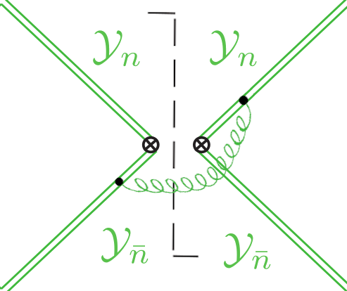
We can define the soft function as a squared matrix element of soft Wilson lines Korchemsky:1993uz; Belitsky:1998tc involving a measurement over a complete set of soft states $\ket{X_{s}}$,

$$S_{\text{thr.}}^{r}(z)=\frac{1}{C_{r}}\sum_{X_{s}}{\rm tr}\bra{0}Y^{\dagger\,r}_{\bar{n}}(0)Y^{r}_{n}(0)\delta(\hat{E}^{2}-{Q^{2}(1-z)})\ket{X_{s}}\bra{X_{s}}Y^{\dagger\,r}_{n}(0)Y^{r}_{\bar{n}}(0)\ket{0}\,,$$

(47)

where the operator $\hat{E}$ picks up the total energy of the real emissions, the Wilson lines are taken in the representation $r$ of the scattering partons and along their light-like direction $n,{\bar{n}}$ and $C_{r}$ is the quadratic Casimir of the gauge group for the representation $r$. Note that for the rest of this section, we will drop the label $r$ for the representation, but the following discussion straightforwardly applies to both the case of adjoint and fundamental representation. Explicitly the Wilson lines take the form

$$Y_{n}(x)=\mathbf{P}\exp{\left[ig\int_{-\infty}^{0}\mathrm{d}t\,n\cdot A_{s}(x+tn)\right]}\,.$$

(48)

The contributions to $S_{\text{thr.}}^{r}(z)$ can be represented, order by order in perturbation theory, in terms of cut diagrams and can be calculated in terms of eikonal Feynman rules, see for example figure 2.

The quantities in eq (46) are bare quantities that are individually ultraviolet and infrared divergent, and the divergences manifest themselves as poles in the dimensional regulator $\epsilon$. We implement the renormalisation of the strong coupling constant via the operator ${\bf Z}_{\alpha_{S}}$ (see appendix A), which expresses the bare strong coupling constant in terms of its renormalised counterpart. We absorb infrared singularities of the hard function into $Z_{H}(\mu^{2})$. The threshold PDFs $f^{\text{th}}_{i}(\tau)$ absorb collinear initial state singularities via a standard mass factorization counter term (see appendix B for details).

	$\displaystyle H_{ij}^{B}(\mu^{2})$	$\displaystyle=$	$\displaystyle Z_{H}(\mu^{2}){\bf Z}_{\alpha_{S}}H_{ij}^{B},$
	$\displaystyle f^{\text{th}}_{i}(\tau,\mu^{2})$	$\displaystyle=$	$\displaystyle\Gamma^{r}(\tau)\otimes_{\tau}f_{i}^{\text{th}}(\tau),$
	$\displaystyle S_{\text{thr.}}^{r}(\tau,\mu^{2})$	$\displaystyle=$	$\displaystyle Z_{H}(\mu^{2})^{-1}\Gamma^{r}(\tau)^{-1}\otimes_{\tau}{\bf{Z}}_{\alpha_{S}}S_{\text{thr,}}^{r}(\tau)\otimes_{\tau}\Gamma^{r}(\tau)^{-1}.$		(49)

Note, that we indicate renormalized and finite objects by explicitly indicating their dependence on the scale $\mu^{2}$.

In the context of SCET, the divergences appearing in the bare soft function can be interpreted as UV divergences in the effective theory. Therefore, we can absorbe these divergences in an $\overline{\mathrm{MS}}$ counterterm $Z_{S}(z,\mu^{2})$ for this operator and obtain a renormalized soft function. Extracting from eq. (5.1) we find

	$\displaystyle S_{\rm{thr.}}^{r}(z,\mu^{2})$	$\displaystyle=$	$\displaystyle Z_{S}(z,\mu^{2})\otimes_{z}{\bf Z}_{\alpha_{S}}S_{\rm{thr.}}^{r}(z),$
	$\displaystyle Z_{S}(z,\mu^{2})\$	$\displaystyle=$	$\displaystyle Z_{H}(\mu^{2})^{-1}\Gamma^{r}(z)^{-1}\otimes_{z}\Gamma^{r}(z)^{-1}.$		(50)

The hard function obeys the renormalisation group equation (RGE)

	$\displaystyle\mu^{2}\frac{\mathrm{d}}{\mathrm{d}\mu^{2}}H_{ij}^{B}(\mu^{2})$	$\displaystyle=$	$\displaystyle\gamma_{H}^{r}(\alpha_{S}(\mu^{2}),\mu^{2})H_{ij}^{B}(\mu^{2}),$
	$\displaystyle\gamma_{H}^{r}(\alpha_{S}(\mu^{2}),\mu^{2})$	$\displaystyle=$	$\displaystyle\Gamma_{\rm cusp}^{r}(\alpha_{S}(\mu))\ln\frac{Q^{2}}{\mu^{2}}+\frac{1}{2}\gamma_{H}(\alpha_{S}(\mu^{2})).$		(51)

Above $\Gamma_{\text{cusp}}^{r}(\alpha_{S}(\mu^{2}))$ is the cusp anomalous dimension Korchemsky:1993uz. Furthermore, we distinguish $\gamma_{H}^{r}(\alpha_{S}(\mu^{2}))$, the non-cusp part of the anomalous dimension, from the entire anomalous dimension $\gamma_{H}^{r}(\alpha_{S}(\mu^{2}),\mu^{2})$ by the number of arguments. The renormalisation group equation for the threshold PDFs is given by the DGLAP evolution equation Altarelli:1977zs; Dokshitzer:1977sg; Gribov:1972ri in the limit of $z\to 1$. Explicitly, the anomalous dimension of the threshold PDFs is the limit of $z\to 1$ of the Altarelli-Parisi splitting functions:

	$\displaystyle\gamma_{f}^{\text{fundamental}}(z,\alpha_{S}(\mu^{2}))$	$\displaystyle=\lim_{z\to 1}P_{qq}(z,\alpha_{S}(\mu^{2})),$
	$\displaystyle\gamma_{f}^{\text{adjoint}}(z,\alpha_{S}(\mu^{2}))$	$\displaystyle=\lim_{z\to 1}P_{gg}(z,\alpha_{S}(\mu^{2})).$			(52)

With this we find

	$\displaystyle\mu^{2}\frac{\mathrm{d}}{\mathrm{d}\mu^{2}}f^{\text{th}}_{i}(z,\mu^{2})$	$\displaystyle=$	$\displaystyle\gamma_{f}^{r}(z,\alpha_{S}(\mu^{2}))\otimes_{z}f^{\text{th}}_{i}(z,\mu^{2}),$
	$\displaystyle\gamma_{f}^{r}(z,\alpha_{S}(\mu^{2}))$	$\displaystyle=$	$\displaystyle\Gamma_{\text{cusp}}^{r}(\alpha_{S}(\mu^{2}))\left[\frac{1}{1-z}\right]_{+}+\frac{1}{2}\gamma_{f}^{r}(\alpha_{S}(\mu^{2}))\delta(1-z).$		(53)

Above, the plus distribution is defined via its action on a test function as

$$\int_{0}^{1}dz\left[\frac{1}{1-z}\right]_{+}\phi(z)=\int_{0}^{1}dz\left(\frac{1}{1-z}\right)(\phi(z)-\phi(1)).$$

(54)

References

- (1) C. Anastasiou, C. Duhr, F. Dulat, F. Herzog and B. Mistlberger, Higgs Boson Gluon-Fusion Production in QCD at Three Loops, Phys. Rev. Lett. 114 (2015) 212001 [1503.06056].
- (2) C. Duhr, F. Dulat and B. Mistlberger, Higgs Boson Production in Bottom-Quark Fusion to Third Order in the Strong Coupling, Phys. Rev. Lett. 125 (2020) 051804 [1904.09990].
- (3) C. Duhr, F. Dulat and B. Mistlberger, Charged current Drell-Yan production at N3LO, JHEP 11 (2020) 143 [2007.13313].
- (4) C. Duhr, F. Dulat and B. Mistlberger, The Drell-Yan cross section to third order in the strong coupling constant, Phys. Rev. Lett. 125 (2020) 172001 [2001.07717].
- (5) F. Dulat, B. Mistlberger and A. Pelloni, Precision predictions at N3LO for the Higgs boson rapidity distribution at the LHC, Phys. Rev. D99 (2019) 034004 [1810.09462].
- (6) B. Mistlberger, Higgs boson production at hadron colliders at N3LO in QCD, JHEP 05 (2018) 028 [1802.00833].
- (7) C. Duhr and B. Mistlberger, Lepton-pair production at hadron colliders at N3LO in QCD, 2111.10379.
- (8) F. Herzog, B. Ruijl, T. Ueda, J. Vermaseren and A. Vogt, On Higgs decays to hadrons and the R-ratio at N4LO, JHEP 08 (2017) 113 [1707.01044].
- (9) P. Baikov, K. Chetyrkin, J. Kuhn and J. Rittinger, Complete QCD Corrections to Hadronic -Decays, Phys. Rev. Lett. 108 (2012) 222003 [1201.5804].
- (10) M. A. Ebert, B. Mistlberger and G. Vita, The Energy-Energy Correlation in the back-to-back limit at N3LO and N3LL′, 2012.07859.
- (11) L. J. Dixon, M.-X. Luo, V. Shtabovenko, T.-Z. Yang and H. X. Zhu, Analytical Computation of Energy-Energy Correlation at Next-to-Leading Order in QCD, Phys. Rev. Lett. 120 (2018) 102001 [1801.03219].
- (12) L. J. Dixon, I. Moult and H. X. Zhu, Collinear limit of the energy-energy correlator, Phys. Rev. D100 (2019) 014009 [1905.01310].
- (13) J. Ablinger, A. Behring, J. Blümlein, A. De Freitas, A. von Manteuffel and C. Schneider, The 3-loop pure singlet heavy flavor contributions to the structure function and the anomalous dimension, Nucl. Phys. B 890 (2014) 48 [1409.1135].
- (14) J. Ablinger, A. Behring, J. Blümlein, A. De Freitas, A. von Manteuffel and C. Schneider, The three-loop splitting functions and , Nucl. Phys. B922 (2017) 1 [1705.01508].
- (15) J. Blümlein, P. Marquard, C. Schneider and K. Schönwald, The three-loop unpolarized and polarized non-singlet anomalous dimensions from off shell operator matrix elements, Nucl. Phys. B 971 (2021) 115542 [2107.06267].
- (16) S. Moch, J. A. M. Vermaseren and A. Vogt, The Three loop splitting functions in QCD: The Nonsinglet case, Nucl. Phys. B688 (2004) 101 [hep-ph/0403192].
- (17) A. Vogt, S. Moch and J. A. M. Vermaseren, The Three-loop splitting functions in QCD: The Singlet case, Nucl. Phys. B691 (2004) 129 [hep-ph/0404111].
- (18) J. M. Henn, G. P. Korchemsky and B. Mistlberger, The full four-loop cusp anomalous dimension in super Yang-Mills and QCD, JHEP 04 (2020) 018 [1911.10174].
- (19) A. von Manteuffel, E. Panzer and R. M. Schabinger, Cusp and collinear anomalous dimensions in four-loop QCD from form factors, Phys. Rev. Lett. 124 (2020) 162001 [2002.04617].
- (20) O. Almelid, C. Duhr, E. Gardi, A. McLeod and C. D. White, Bootstrapping the QCD soft anomalous dimension, JHEP 09 (2017) 073 [1706.10162].
- (21) O. Almelid, C. Duhr and E. Gardi, Three-loop corrections to the soft anomalous dimension in multileg scattering, Phys. Rev. Lett. 117 (2016) 172002 [1507.00047].
- (22) C. Anastasiou, S. Buehler, C. Duhr and F. Herzog, NNLO phase space master integrals for two-to-one inclusive cross sections in dimensional regularization, JHEP 11 (2012) 062 [1208.3130].
- (23) C. Anastasiou, C. Duhr, F. Dulat and B. Mistlberger, Soft triple-real radiation for Higgs production at N3LO, JHEP 07 (2013) 003 [1302.4379].
- (24) C. Anastasiou, C. Duhr, F. Dulat, E. Furlan, F. Herzog and B. Mistlberger, Soft expansion of double-real-virtual corrections to Higgs production at N3LO, JHEP 08 (2015) 051 [1505.04110].
- (25) C. Anastasiou, C. Duhr, F. Dulat, E. Furlan, T. Gehrmann, F. Herzog et al., Higgs Boson Gluon Fusion Production Beyond Threshold in N QCD, JHEP 03 (2015) 091 [1411.3584].
- (26) C. Anastasiou and K. Melnikov, Higgs boson production at hadron colliders in NNLO QCD, Nuclear Physics B 646 (2002) 220 [0207004].
- (27) C. Anastasiou and K. Melnikov, Pseudoscalar Higgs boson production at hadron colliders in next-to-next-to-leading order QCD, Physical Review D 67 (2003) 037501.
- (28) C. Anastasiou, L. Dixon and K. Melnikov, NLO Higgs boson rapidity distributions at hadron colliders, Nuclear Physics B - Proceedings Supplements 116 (2003) 193.
- (29) C. Anastasiou, L. Dixon, K. Melnikov and F. Petriello, Dilepton Rapidity Distribution in the Drell-Yan Process at Next-to-Next-to-Leading Order in QCD, Physical Review Letters 91 (2003) 182002.
- (30) C. Anastasiou, L. Dixon, K. Melnikov and F. Petriello, High-precision QCD at hadron colliders: Electroweak gauge boson rapidity distributions at next-to-next-to leading order, Physical Review D 69 (2004) 094008.
- (31) C. Anastasiou, C. Duhr, F. Dulat, E. Furlan, T. Gehrmann, F. Herzog et al., Higgs boson gluonfusion production at threshold in N3LO QCD, Phys. Lett. B737 (2014) 325 [1403.4616].
- (32) C. Anastasiou, C. Duhr, F. Dulat, F. Herzog and B. Mistlberger, Real-virtual contributions to the inclusive Higgs cross-section at , JHEP 12 (2013) 088 [1311.1425].
- (33) A. Kotikov, Differential equations method: New technique for massive Feynman diagrams calculation, Phys. Lett. B 254 (1991) 158.
- (34) A. Kotikov, Differential equations method: The Calculation of vertex type Feynman diagrams, Phys. Lett. B 259 (1991) 314.
- (35) A. Kotikov, Differential equation method: The Calculation of N point Feynman diagrams, Phys. Lett. B 267 (1991) 123.
- (36) T. Gehrmann and E. Remiddi, Differential equations for two loop four point functions, Nucl. Phys. B580 (2000) 485 [hep-ph/9912329].
- (37) J. M. Henn, Multiloop integrals in dimensional regularization made simple, Phys. Rev. Lett. 110 (2013) 251601 [1304.1806].
- (38) C. Duhr, F. Dulat, V. Hirschi and B. Mistlberger, Higgs production in bottom quark fusion: matching the 4- and 5-flavour schemes to third order in the strong coupling, JHEP 08 (2020) 017 [2004.04752].
- (39) F. Dulat, S. Lionetti, B. Mistlberger, A. Pelloni and C. Specchia, Higgs-differential cross section at NNLO in dimensional regularisation, JHEP 07 (2017) 017 [1704.08220].
- (40) F. Dulat, B. Mistlberger and A. Pelloni, Differential Higgs production at N3LO beyond threshold, JHEP 01 (2018) 145 [1710.03016].
- (41) M. A. Ebert, B. Mistlberger and G. Vita, Collinear expansion for color singlet cross sections, JHEP 09 (2020) 181 [2006.03055].
- (42) M. A. Ebert, B. Mistlberger and G. Vita, Transverse momentum dependent PDFs at N3LO, JHEP 09 (2020) 146 [2006.05329].
- (43) M. A. Ebert, B. Mistlberger and G. Vita, -jettiness beam functions at N3LO, JHEP 09 (2020) 143 [2006.03056].
- (44) M. A. Ebert, B. Mistlberger and G. Vita, TMD fragmentation functions at N3LO, JHEP 07 (2021) 121 [2012.07853].
- (45) F. Dulat and B. Mistlberger, Real-Virtual-Virtual contributions to the inclusive Higgs cross section at N3LO, 1411.3586.
- (46) C. Duhr and T. Gehrmann, The two-loop soft current in dimensional regularization, Phys. Lett. B727 (2013) 452 [1309.4393].
- (47) C. Duhr, T. Gehrmann and M. Jaquier, Two-loop splitting amplitudes and the single-real contribution to inclusive Higgs production at N3LO, JHEP 02 (2015) 077 [1411.3587].
- (48) G. F. Sterman, Summation of Large Corrections to Short Distance Hadronic Cross-Sections, Nucl. Phys. B 281 (1987) 310.
- (49) S. Catani, D. de Florian, M. Grazzini and P. Nason, Soft gluon resummation for Higgs boson production at hadron colliders, JHEP 07 (2003) 028 [hep-ph/0306211].
- (50) S. Catani and L. Trentadue, Resummation of the QCD Perturbative Series for Hard Processes, Nucl. Phys. B 327 (1989) 323.
- (51) S. Catani and L. Trentadue, Comment on QCD exponentiation at large x, Nucl. Phys. B 353 (1991) 183.
- (52) V. Ahrens, T. Becher, M. Neubert and L. L. Yang, Renormalization-Group Improved Prediction for Higgs Production at Hadron Colliders, Eur. Phys. J. C 62 (2009) 333 [0809.4283].
- (53) V. Ahrens, T. Becher, M. Neubert and L. L. Yang, Origin of the Large Perturbative Corrections to Higgs Production at Hadron Colliders, Phys. Rev. D 79 (2009) 033013 [0808.3008].
- (54) V. Ahrens, T. Becher, M. Neubert and L. L. Yang, Updated Predictions for Higgs Production at the Tevatron and the LHC, Phys. Lett. B 698 (2011) 271 [1008.3162].
- (55) G. Das, S. Moch and A. Vogt, Approximate four-loop QCD corrections to the Higgs-boson production cross section, Phys. Lett. B 807 (2020) 135546 [2004.00563].
- (56) A. Vogt, F. Herzog, S. Moch, B. Ruijl, T. Ueda and J. A. M. Vermaseren, Anomalous dimensions and splitting functions beyond the next-to-next-to-leading order, PoS LL2018 (2018) 050 [1808.08981].
- (57) S. Moch, B. Ruijl, T. Ueda, J. A. M. Vermaseren and A. Vogt, Four-Loop Non-Singlet Splitting Functions in the Planar Limit and Beyond, JHEP 10 (2017) 041 [1707.08315].
- (58) S. Moch, B. Ruijl, T. Ueda, J. A. M. Vermaseren and A. Vogt, Low moments of the four-loop splitting functions in QCD, Phys. Lett. B 825 (2022) 136853 [2111.15561].
- (59) S. Moch, B. Ruijl, T. Ueda, J. A. M. Vermaseren and A. Vogt, On quartic colour factors in splitting functions and the gluon cusp anomalous dimension, Phys. Lett. B 782 (2018) 627 [1805.09638].
- (60) G. Das, S.-O. Moch and A. Vogt, Soft corrections to inclusive deep-inelastic scattering at four loops and beyond, JHEP 03 (2020) 116 [1912.12920].
- (61) M. Beneke and V. A. Smirnov, Asymptotic expansion of Feynman integrals near threshold, Nucl. Phys. B522 (1998) 321 [hep-ph/9711391].
- (62) F. Tkachov, A theorem on analytical calculability of 4-loop renormalization group functions, Physics Letters B 100 (1981) 65.
- (63) K. Chetyrkin and F. Tkachov, Integration by parts: The algorithm to calculate -functions in 4 loops, Nuclear Physics B 192 (1981) 159.
- (64) S. Laporta, High precision calculation of multiloop Feynman integrals by difference equations, Int. J. Mod. Phys. A15 (2000) 5087 [hep-ph/0102033].
- (65) R. N. Lee, Multiloop calculations with differential equations in -form, EPJ Web Conf. 125 (2016) 05020.
- (66) J. Henn, B. Mistlberger, V. A. Smirnov and P. Wasser, Constructing d-log integrands and computing master integrals for three-loop four-particle scattering, JHEP 04 (2020) 167 [2002.09492].
- (67) E. Remiddi and J. A. M. Vermaseren, Harmonic polylogarithms, Int. J. Mod. Phys. A15 (2000) 725 [hep-ph/9905237].
- (68) T. Huber and D. Maitre, HypExp: A Mathematica package for expanding hypergeometric functions around integer-valued parameters, Comput. Phys. Commun. 175 (2006) 122 [hep-ph/0507094].
- (69) G. Somogyi, Angular integrals in d dimensions, J. Math. Phys. 52 (2011) 083501 [1101.3557].
- (70) M. Czakon, Automatized analytic continuation of Mellin-Barnes integrals, Comput. Phys. Commun. 175 (2006) 559 [hep-ph/0511200].
- (71) A. V. Smirnov and V. A. Smirnov, On the Resolution of Singularities of Multiple Mellin-Barnes Integrals, Eur. Phys. J. C 62 (2009) 445 [0901.0386].
- (72) K. G. Chetyrkin, B. A. Kniehl and M. Steinhauser, Decoupling relations to and their connection to low-energy theorems, Nucl. Phys. B510 (1998) 61 [hep-ph/9708255].
- (73) Y. Schroder and M. Steinhauser, Four-loop decoupling relations for the strong coupling, JHEP 01 (2006) 051 [hep-ph/0512058].
- (74) K. Chetyrkin, J. Kühn and C. Sturm, QCD decoupling at four loops, Nuclear Physics B 744 (2006) 121.
- (75) M. Kramer, E. Laenen and M. Spira, Soft gluon radiation in Higgs boson production at the LHC, Nucl. Phys. B511 (1998) 523 [hep-ph/9611272].
- (76) T. Inami, T. Kubota and Y. Okada, Effective Gauge Theory and the Effect of Heavy Quarks, Zeitschrift für Physik C 18 (1983) 69.
- (77) M. Shifman, A. Vainshtein and V. Zakharov, Remarks on Higgs-boson interactions with nucleons, Physics Letters B 78 (1978) 443.
- (78) V. P. Spiridonov and K. G. Chetyrkin, Nonleading mass corrections and renormalization of the operators m psi-bar psi and g**2(mu nu), Sov. J. Nucl. Phys. 47 (1988) 522.
- (79) F. Wilczek, Decays of Heavy Vector Mesons into Higgs Particles, Physical Review Letters 39 (1977) 1304.
- (80) T. Gehrmann, T. Huber and D. Maitre, Two-loop quark and gluon form-factors in dimensional regularisation, Phys. Lett. B 622 (2005) 295 [hep-ph/0507061].
- (81) P. A. Baikov, K. G. Chetyrkin, A. V. Smirnov, V. A. Smirnov and M. Steinhauser, Quark and gluon form factors to three loops, Phys. Rev. Lett. 102 (2009) 212002 [0902.3519].
- (82) T. Gehrmann, E. W. N. Glover, T. Huber, N. Ikizlerli and C. Studerus, Calculation of the quark and gluon form factors to three loops in QCD, JHEP 06 (2010) 094 [1004.3653].
- (83) T. Gehrmann, E. W. N. Glover, T. Huber, N. Ikizlerli and C. Studerus, The quark and gluon form factors to three loops in QCD through to O(eps2), JHEP 11 (2010) 102 [1010.4478].
- (84) B. Agarwal, A. von Manteuffel, E. Panzer and R. M. Schabinger, Four-loop collinear anomalous dimensions in QCD and N=4 super Yang-Mills, Phys. Lett. B 820 (2021) 136503 [2102.09725].
- (85) R. N. Lee, A. von Manteuffel, R. M. Schabinger, A. V. Smirnov, V. A. Smirnov and M. Steinhauser, Fermionic corrections to quark and gluon form factors in four-loop QCD, Phys. Rev. D 104 (2021) 074008 [2105.11504].
- (86) R. N. Lee, A. von Manteuffel, R. M. Schabinger, A. V. Smirnov, V. A. Smirnov and M. Steinhauser, Quark and gluon form factors in four-loop QCD, 2202.04660.
- (87) Y. Li, A. von Manteuffel, R. M. Schabinger and H. X. Zhu, Soft-virtual corrections to Higgs production at N3LO, Phys. Rev. D91 (2015) 036008 [1412.2771].
- (88) T. Ahmed, M. Mahakhud, N. Rana and V. Ravindran, Drell-Yan Production at Threshold to Third Order in QCD, Phys. Rev. Lett. 113 (2014) 112002 [1404.0366].
- (89) S. Catani and M. Grazzini, The soft gluon current at one loop order, Nucl. Phys. B 591 (2000) 435 [hep-ph/0007142].
- (90) Y. Li and H. X. Zhu, Single soft gluon emission at two loops, JHEP 11 (2013) 080 [1309.4391].
- (91) L. J. Dixon, E. Herrmann, K. Yan and H. X. Zhu, Soft gluon emission at two loops in full color, JHEP 05 (2020) 135 [1912.09370].
- (92) C. W. Bauer, S. Fleming and M. E. Luke, Summing Sudakov logarithms in in effective field theory, Phys. Rev. D63 (2000) 014006 [hep-ph/0005275].
- (93) C. W. Bauer, S. Fleming, D. Pirjol and I. W. Stewart, An Effective field theory for collinear and soft gluons: Heavy to light decays, Phys. Rev. D63 (2001) 114020 [hep-ph/0011336].
- (94) C. W. Bauer and I. W. Stewart, Invariant operators in collinear effective theory, Phys. Lett. B516 (2001) 134 [hep-ph/0107001].
- (95) C. W. Bauer, D. Pirjol and I. W. Stewart, Soft collinear factorization in effective field theory, Phys. Rev. D65 (2002) 054022 [hep-ph/0109045].
- (96) C. W. Bauer, S. Fleming, D. Pirjol, I. Z. Rothstein and I. W. Stewart, Hard scattering factorization from effective field theory, Phys. Rev. D66 (2002) 014017 [hep-ph/0202088].
- (97) G. P. Korchemsky and G. Marchesini, Resummation of large infrared corrections using Wilson loops, Phys. Lett. B 313 (1993) 433.
- (98) A. V. Belitsky, Two loop renormalization of Wilson loop for Drell-Yan production, Phys. Lett. B 442 (1998) 307 [hep-ph/9808389].
- (99) G. Altarelli and G. Parisi, Asymptotic Freedom in Parton Language, Nucl. Phys. B126 (1977) 298.
- (100) Y. L. Dokshitzer, Calculation of the Structure Functions for Deep Inelastic Scattering and e+ e- Annihilation by Perturbation Theory in Quantum Chromodynamics., Sov. Phys. JETP 46 (1977) 641.
- (101) V. N. Gribov and L. N. Lipatov, Deep inelastic e p scattering in perturbation theory, Sov. J. Nucl. Phys. 15 (1972) 438.
- (102) P. A. Baikov, K. G. Chetyrkin and J. H. Kühn, Five-Loop Running of the QCD coupling constant, Phys. Rev. Lett. 118 (2017) 082002 [1606.08659].
- (103) F. Herzog, B. Ruijl, T. Ueda, J. A. M. Vermaseren and A. Vogt, The five-loop beta function of Yang-Mills theory with fermions, JHEP 02 (2017) 090 [1701.01404].
- (104) T. van Ritbergen, J. A. M. Vermaseren and S. A. Larin, The Four loop beta function in quantum chromodynamics, Phys. Lett. B400 (1997) 379 [hep-ph/9701390].
- (105) M. Czakon, The Four-loop QCD beta-function and anomalous dimensions, Nucl. Phys. B710 (2005) 485 [hep-ph/0411261].
- (106) O. V. Tarasov, A. A. Vladimirov and A. Yu. Zharkov, The Gell-Mann-Low Function of QCD in the Three Loop Approximation, Phys. Lett. 93B (1980) 429.
- (107) S. A. Larin and J. A. M. Vermaseren, The Three loop QCD Beta function and anomalous dimensions, Phys. Lett. B303 (1993) 334 [hep-ph/9302208].
- (108) S. Moch, J. A. M. Vermaseren and A. Vogt, On 5 in higher-order QCD calculations and the NNLO evolution of the polarized valence distribution, Phys. Lett. B 748 (2015) 432 [1506.04517].
- (109) S. Moch, J. A. M. Vermaseren and A. Vogt, The Three-Loop Splitting Functions in QCD: The Helicity-Dependent Case, Nucl. Phys. B 889 (2014) 351 [1409.5131].
- (110) I. W. Stewart, F. J. Tackmann and W. J. Waalewijn, N-Jettiness: An Inclusive Event Shape to Veto Jets, Phys. Rev. Lett. 105 (2010) 092002 [1004.2489].
- (111) I. W. Stewart, F. J. Tackmann and W. J. Waalewijn, The Quark Beam Function at NNLL, JHEP 09 (2010) 005 [1002.2213].
- (112) T. Becher, M. Neubert and B. D. Pecjak, Factorization and Momentum-Space Resummation in Deep-Inelastic Scattering, JHEP 01 (2007) 076 [hep-ph/0607228].
- (113) T. Becher and M. D. Schwartz, A precise determination of from LEP thrust data using effective field theory, JHEP 07 (2008) 034 [0803.0342].
- (114) R. Abbate, M. Fickinger, A. H. Hoang, V. Mateu and I. W. Stewart, Thrust at N3LL with Power Corrections and a Precision Global Fit for , Phys. Rev. D83 (2011) 074021 [1006.3080].
- (115) R. Abbate, M. Fickinger, A. H. Hoang, V. Mateu and I. W. Stewart, Precision Thrust Cumulant Moments at LL, Phys. Rev. D 86 (2012) 094002 [1204.5746].
- (116) G. Lustermans, J. K. L. Michel and F. J. Tackmann, Generalized Threshold Factorization with Full Collinear Dynamics, 1908.00985.