Linear Runlength-Limited Subcodes of Reed-Muller Codes and Coding Schemes for Input-Constrained BMS Channels

The physical limitations of hardware used in most data recording and communication systems cause some sequences to be more prone to error than others. Constrained coding is a method of alleviating this problem, by encoding arbitrary user data sequences into sequences that respect a constraint (see, for example, [1] or [2]). In this work, we investigate the sizes of linear subcodes of well-known families of codes, all of whose codewords obey a certain hard constraint. In particular, we work with the binary Reed-Muller (RM) family of codes and obtain upper bounds on the sizes of linear subcodes that obey a runlength-limited (RLL) constraint.

The specific hard constraint of interest to us is the $(d,\infty)$-RLL constraint, which admits only binary sequences with at least $d$ $0$s between every pair of successive $1$s. Figure 2 shows a state transition graph that represents the constraint. This constraint is a special case of the $(d,k)$-RLL constraint, which admits only binary sequences with at least $d$ and at most $k$ $0$s between successive $1$s.

One of the motivations for studying this problem is the design of explicit coding schemes that achieve good rates over input-constrained discrete memoryless channels (DMCs). Figure 2 shows a generic binary memoryless symmetric (BMS) channel with input constraints. Input-constrained DMCs in general fall under the broad class of discrete finite-state channels (DFSCs, or FSCs).

While explicit codes achieving the capacities or whose rates are very close to the capacities of unconstrained DMCs have been derived in works such as [3, 4, 5, 6, 7], the problem of designing coding schemes for input-constrained DMCs has not received much attention in the literature. Moreover, unlike the case of the unconstrained DMC, whose capacity is characterized by Shannon’s single-letter, computable formula, $C_{\text{DMC}}=\sup_{P(x)}I(X;Y)$, the explicit computation of the capacity of an FSC is a much more difficult problem to tackle.

With the recent result of Reeves and Pfister [8] that Reed-Muller (RM) codes achieve the capacity of the unconstrained BMS channel under bit-MAP decoding, there opens the possibility of using such algebraic codes over input-constrained BMS channels as well. Suppose that $C$ is the capacity of the unconstrained channel. The authors in [9] showed a simple linear coding scheme, using subcodes of RM codes, with rates of $C\cdot{2^{-\left\lceil\log_{2}(d+1)\right\rceil}}$, being achievable over $(d,\infty)$-RLL input-constrained BMS channels. In this paper, we prove that any linear RM subcode that respects the $(d,\infty)$-RLL constraint, must have a rate of at most $\frac{C}{d+1}$, in the limit as the blocklength goes to infinity. In doing so, we show that one cannot do better, asymptotically, than the simple coding scheme in [9], if one requires that the subcodes be linear. We also consider the rates achieved using linear $(d,\infty)$-RLL subcodes of permuted RM codes, and show that for codes of large enough blocklength, almost all permutations must respect an upper bound of $\frac{C}{d+1}+\delta$, for $\delta$ being as small as is required.

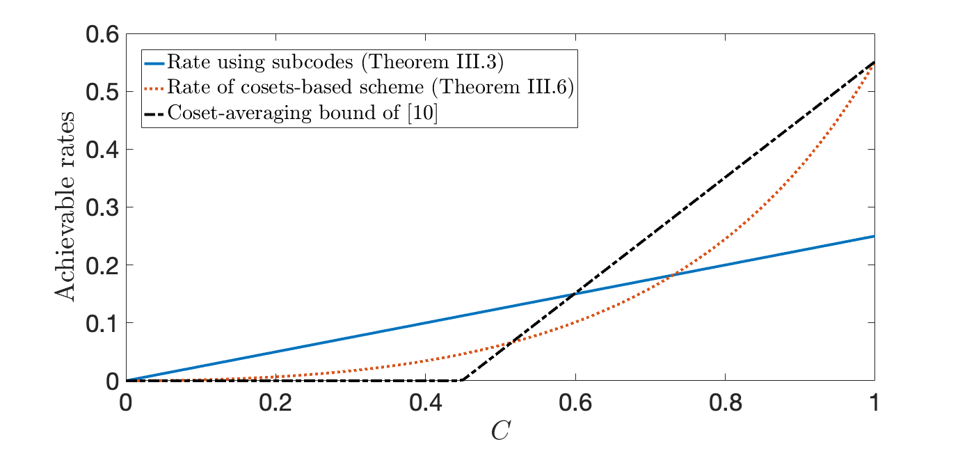
As an improvement over the rates achievable using linear $(d,\infty)$-RLL subcodes of RM codes, we propose a new coding scheme that uses cosets of RM codes. The rate achieved by this scheme is $\frac{C_{0}\cdot C^{2}\cdot 2^{-\left\lceil\log_{2}(d+1)\right\rceil}}{C^{2}\cdot 2^{-\left\lceil\log_{2}(d+1)\right\rceil}+1-C+\epsilon}$, where $C_{0}$ is the noiseless capacity of the input constraint, and $\epsilon>0$ can be taken to be as small as is required. For example, when $d=1$, the rates achieved using this cosets-based scheme are better than those achieved by any scheme that uses linear $(1,\infty)$-RLL subcodes of RM codes, when $C\gtrapprox 0.7613$. Moreover, as the capacity of the channel approaches $1$, i.e., as the channel noise approaches $0$, the rate achieved by our cosets-based scheme approaches a value arbitrarily close to $C_{0}$, which is the largest rate achievable, at zero noise, given the constraint.

Our results supplement the analysis in [10], on rates achievable by $(d,k)$-RLL subcodes of cosets of a linear block code. Specifically, Corollary 1 of [10] provides an existence result on cosets of capacity-achieving (over the unconstrained BMS channel) codes, whose constrained subcodes have rate at least $C_{0}+C-1$. The coding scheme in this paper achieves rates close to the lower bound in [10], for values of $C$ close to $1$. We note that using linear $(d,\infty)$-RLL subcodes of RM codes as in [9], we can achieve larger rates as compared to the rate lower bound in [10], when the capacity $C$ is low, i.e., when $C<(1-C_{0})\cdot\left(1-{2^{-\left\lceil\log_{2}(d+1)\right\rceil}}\right)^{-1}$.

The remainder of the paper is organized as follows: Section II introduces the notation and provides the necessary background. Section III states our main results. Section IV discusses upper bounds on the rate achievable over the BMS channel, using linear $(d,\infty)$-RLL subcodes. In Section V, the question of upper bounds on rates achievable using linear $(d,\infty)$-RLL subcodes, under coordinate orderings different from the standard lexicographic ordering, is taken up. Section VI then discusses a construction that uses cosets of RM codes to achieve good rates. Finally, Section VII contains concluding remarks and a discussion on possible future work.

Before we state our upper bound on the rates of linear RLL subcodes of RM codes, we recall the result of Reeves and Pfister in [8], which provides context to our using RM codes over input-constrained BMS channels. For a given $R\in(0,1)$, consider any sequence of RM codes $\{\mathcal{C}_{m}(R)=\text{RM}(m,r_{m})\}_{m\geq 1}$, under the lexicographic ordering of coordinates, with $R_{m}$ being the rate of $\mathcal{C}_{m}(R)$, such that $R_{m}\to R$ as $m\to\infty$. The following theorem then holds true:

Hence, the families of codes described above are $(0,\infty)$-capacity-achieving, under bit-MAP decoding.

We now discuss a theorem that provides upper bounds on the largest rate achievable, using linear subcodes of RM codes, over a $(d,\infty)$-RLL input-constrained BMS channel. Fix any sequence of codes $\{{\mathcal{C}}_{m}(R)=\text{RM}(m,r_{m})\}_{m\geq 1}$, which achieves a rate $R$ over the unconstrained BMS channel. Let $\overline{\mathcal{C}}_{d}^{(m)}$ denote the largest linear subcode of ${\mathcal{C}}_{m}(R)$, all of whose codewords respect the $(d,\infty)$-RLL constraint. We then define

to be the largest rate achieved by linear $(d,\infty)$-RLL subcodes of $\{{C}_{m}(R)\}$, assuming that the ordering of the coordinates of the code is according to the lexicographic ordering. Then,

Hence, from Theorem III.1, the largest rate achievable over a $(d,\infty)$-RLL input-constrained BMS channel, under bit-MAP decoding, using linear $(d,\infty)$-RLL subcodes of RM codes, is bounded above by $\frac{C}{d+1}$, where $C$ is the capacity of the unconstrained BMS channel. Theorem III.2 is proved in Section IV. Now, consider the sequence of RM codes $\{\hat{\mathcal{C}}_{m}(R)=\text{RM}(m,v_{m})\}_{m\geq 1}$, with

where $Q(\cdot)$ is the complementary cumulative distribution function (c.c.d.f.) of the standard normal distribution.

Now, for a fixed $d\geq 1$, let $z:=\left\lceil\log_{2}(d+1)\right\rceil$. Consider the subcode $\mathcal{C}_{m}^{(d,\infty)}(R)$, of the code $\mathcal{C}_{m}(R)$, defined as:

Note that $\mathcal{C}_{m}^{(d,\infty)}(R)$ is a linear subcode of $\mathcal{C}_{m}(R)$. The following theorem from [9] then holds:

Thus, Theorem III.2 shows that the sequence of linear subcodes $\{{\mathcal{C}}_{m}^{(d,\infty)}(R)\}_{m\geq 1}$, in equation (III), is rate-optimal whenever $d+1$ is a power of $2$, in that it achieves the rate upper bound of $R/(d+1)$. We remark here that the problem of identifying linear codes that are subsets of the set of $(d,\infty)$-RLL sequences of a fixed length, has been studied [13]. The results therein show that the largest linear code within $S_{(d,\infty)}^{(m)}$ has rate no larger than $\frac{1}{d+1}$, as $m\to\infty$. However, such a result offers no insight into rates achievable over BMS channels.

We then consider situations where the coordinates of the RM codes follow orderings different from the standard lexicographic ordering. First, we study upper bounds on the rates of linear $(d,\infty)$-RLL subcodes of RM codes, ordered according to a Gray ordering (see Section V for a description of a Gray ordering). For a fixed $R\in(0,C)$, let $\{{\mathcal{C}}_{m}^{\text{G}}(R)\}_{m\geq 1}$ be any sequence of RM codes under a Gray ordering, such that rate$(\mathcal{C}_{m}^{\text{G}}(R))\xrightarrow{m\to\infty}R$. Further, for every $m$, let $\overline{\mathcal{C}}_{d,\text{G}}^{(m)}$ be the largest linear subcode of ${\mathcal{C}}_{m}^{\text{G}}(R)$. We also define

to be the largest rate achieved by linear $(d,\infty)$-RLL subcodes of $\{\mathcal{C}_{m}^{\text{G}}(R)\}_{m\geq 1}$. We obtain the following result:

The proof of Theorem III.4 is provided in Section V.

Now, we consider arbitrary orderings of coordinates, defined by the sequence of permutations $(\pi_{m})_{m\geq 1}$, with $\pi_{m}:[0:2^{m}-1]\to[0:2^{m}-1]$. As with the Gray ordering, we define the sequence of $\pi$-ordered RM codes $\{\mathcal{C}_{m}^{\pi}(R)\}_{m\geq 1}$, with

We also define $\overline{\mathcal{C}}_{d,\pi}^{(m)}$ be the largest linear $(d,\infty)$-RLL subcode of $\mathcal{C}_{m}^{\pi}(R)$. The theorem below is then shown to hold:

Section V contains the proof of Theorem III.5.

Next, we turn our attention to the design of non-linear $(d,\infty)$-RLL codes, whose rates improve on those in Theorem III.3. Our next theorem, stated below informally, uses cosets of RM codes, for this purpose. We denote by $C_{0}^{(d)}$, the noiseless capacity of the $(d,\infty)$-RLL constraint, and by $C$, the capacity of the unconstrained BMS channel.

It can be checked that the rates achieved using Theorem III.6 are better than those achieved using Theorem III.3 (and in fact, better than those achieved using any sequence of linear $(d,\infty)$-RLL subcodes of RM codes), for low noise regimes of the BMS channel. For example, when $d=1$, the rates achieved using the codes in Theorem III.6 are better than those achieved using linear subcodes, for certain values of $C\gtrapprox 0.7613$. Figures 4 and 5 show comparisons between the lower bounds (achievable rates) in Theorems III.3 and III.6, with the coset-averaging bound of [10], for $d=1$ and $d=2$, respectively. While [10] provides existence results on rates achieved using cosets of RM codes, with the rates calculated therein being better than those in Theorem III.6 in the low noise regimes of the BMS channel, our construction is more explicit. A discussion on the construction leading to Theorem III.6 is taken up in Section VI.

We end this section with a remark. Note that the all-ones codeword $\mathbf{1}$ belongs to any RM code. Since any codeword $\mathbf{c}$ that respects the $(0,1)$-RLL constraint can be written as $\mathbf{c}=\mathbf{1}+\mathbf{\hat{c}}$, where $\mathbf{\hat{c}}$ respects the $(1,\infty)$-RLL constraint, the lower bound of Theorem III.3 and the upper bound of Theorem III.2 hold for the rates of $(0,1)$-RLL subcodes as well.

In this section, we derive upper bounds on the rates achieved by linear $(d,\infty)$-RLL subcodes of any sequence of RM codes of rate $R$. We fix a sequence of codes $\{{\mathcal{C}_{m}(R)}=\text{RM}(m,r_{m})\}$ that achieves a rate $R$ over the unconstrained BMS channel.

We first state and prove a fairly general proposition on the rates of linear $(d,\infty)$-RLL subcodes of linear codes. Recall that for a linear code $\mathcal{C}$ over $\mathbb{F}_{2}$, of blocklength $N$ and dimension $K$, an information set is a collection of $K$ coordinates in which all possible $K$-tuples over $\mathbb{F}_{2}$ can appear. Equivalently, if $G$ is any generator matrix for $\mathcal{C}$, an information set is a set of $K$ column indices such that $G$ restricted to those columns is a full-rank matrix.

In order to obtain an upper bound, as in Theorem III.2, on the rate of linear $(d,\infty)$-RLL subcodes of the sequence of codes $\{{\mathcal{C}_{m}(R)}\}_{m\geq 1}$, we shall first identify an information set $\mathcal{I}_{m,r_{m}}$ of ${\mathcal{C}_{m}(R)}=\text{RM}(m,r_{m})$. We then compute the number of disjoint $(d+1)$-tuples of consecutive coordinates in $\mathcal{I}_{m,r_{m}}$, and apply Proposition IV.1 to get an upper bound on the dimension of the linear constrained subcodes.

We introduce some notation for ease of reading: given a matrix $M_{p\times q}$, we use the notation $M[\mathcal{U},\mathcal{V}]$ to denote the submatrix of $M$ consisting of the rows in the set $\mathcal{U}\subseteq[p]$ and the columns in the set $\mathcal{V}\subseteq[q]$. We also recall the definition of the generator matrix $G_{\text{Lex}}(m,r)$, of RM$(m,r)$, and the indexing of columns of the matrix, from Section II-B. We also interchangeably index the coordinates of a codeword of RM$(m,r)$ by integers $i\in[0,2^{m}-1]$, and by $m$-tuples of binary symbols. Further, the notation $\mathbf{e}_{\mathbf{b}}^{(2^{m})}$ denotes the standard basis vector with a $1$ in the coordinate indexed by $\mathbf{b}=(b_{1},\ldots,b_{m})$, in the lexicographic order. The superscript ‘$(2^{m})$’ will be dropped when clear from the context.

Now, given the code RM$(m,r)$, consider the binary linear code (a subspace of $\mathbb{F}_{2}^{2^{m}}$), $\tilde{\mathcal{C}}({m,r})$, spanned by the codewords in the set

It can be checked that the vectors in $\mathcal{B}_{m,r}$ are also linearly independent, and, hence, $\mathcal{B}_{m,r}$ forms a basis for $\tilde{\mathcal{C}}({m,r})$, with dim$\left(\tilde{\mathcal{C}}({m,r})\right)={m\choose\geq r+1}$. Moreover, the codewords in $\tilde{\mathcal{C}}({m,r})$ are linearly independent from codewords in RM$(m,r)$, by definition.

The following lemma identifies an alternative basis for $\tilde{\mathcal{C}}({m,r})$, which will prove useful in our analysis, later on.

Now that we have identified an information set $\mathcal{I}_{m,r_{m}}$ of $\mathcal{C}_{m}(R)=$ RM$(m,r_{m})$, we need only calculate the number of disjoint $(d+1)$-tuples of consecutive coordinates in $\mathcal{I}_{m,r_{m}}$. We introduce the notation B$(i)$ to denote the length-$m$ binary representation of $i$, for $0\leq i\leq 2^{m}-1$. We also define a “run” of coordinates belonging to a set $\mathcal{A}\in\{0,1\}^{m}$, to be a contiguous collection of coordinates, $\left(i,i+1,\ldots,i+\ell\right)$, such that $\mathbf{B}(j)\in\mathcal{A}$, for all $i\leq j\leq i+\ell$, and $\mathbf{B}(i-1),\mathbf{B}(i+\ell+1)\notin\mathcal{A}$, where $i\in[0:2^{m}-1-\ell]$. Further, the length of such a run of coordinates is exactly $\ell$.

We shall first compute the number of runs of consecutive coordinates, in the lexicographic ordering, which belong to the information set $\mathcal{I}_{m,r_{m}}$. Formally, if we define

to be the set of right end-point coordinates of runs that belong to $\mathcal{I}_{m,r_{m}}$, then the required number of runs is $\left\lvert\Gamma_{m,r_{m}}\right\rvert$.

With the ingredients in place, we are now in a position to prove Theorem III.2.

References

- [1] B. H. Marcus, R. M. Roth, and P. H. Siegel, “An introduction to coding for constrained systems,” Lecture notes, 2001.
- [2] K. A. S. Immink, P. H. Siegel, and J. K. Wolf, “Codes for digital recorders,” IEEE Transactions on Information Theory, vol. 44, no. 6, pp. 2260–2299, Oct. 1998.
- [3] E. Arikan, “Channel polarization: A method for constructing capacity-achieving codes for symmetric binary-input memoryless channels,” IEEE Transactions on Information Theory, vol. 55, no. 7, pp. 3051–3073, 2009.
- [4] S. Kudekar, S. Kumar, M. Mondelli, H. D. Pfister, E. Şaşoǧlu, and R. L. Urbanke, “Reed–Muller codes achieve capacity on erasure channels,” IEEE Transactions on Information Theory, vol. 63, no. 7, pp. 4298–4316, 2017.
- [5] M. Luby, M. Mitzenmacher, M. Shokrollahi, and D. Spielman, “Efficient erasure correcting codes,” IEEE Transactions on Information Theory, vol. 47, no. 2, pp. 569–584, 2001.
- [6] T. Richardson, M. Shokrollahi, and R. Urbanke, “Design of capacity-approaching irregular low-density parity-check codes,” IEEE Transactions on Information Theory, vol. 47, no. 2, pp. 619–637, 2001.
- [7] S. Kudekar, T. Richardson, and R. L. Urbanke, “Spatially coupled ensembles universally achieve capacity under belief propagation,” IEEE Transactions on Information Theory, vol. 59, no. 12, pp. 7761–7813, 2013.
- [8] G. Reeves and H. D. Pfister, “Reed-Muller codes achieve capacity on BMS channels,” arXiv e-prints, p. arXiv:2110.14631, Oct. 2021.
- [9] V. A. Rameshwar and N. Kashyap, “On the performance of Reed-Muller codes over -RLL input-constrained BMS channels,” arXiv e-prints, p. arXiv:2201.02035, Jan. 2022.
- [10] A. Patapoutian and P. Kumar, “The subcode of a linear block code,” IEEE Transactions on Information Theory, vol. 38, no. 4, pp. 1375–1382, 1992.
- [11] F. MacWilliams and N. Sloane, The Theory of Error-Correcting Codes, 2nd ed. North-holland Publishing Company, 1978.
- [12] E. Abbe, A. Shpilka, and M. Ye, “Reed–Muller codes: Theory and algorithms,” IEEE Transactions on Information Theory, vol. 67, no. 6, pp. 3251–3277, 2021.
- [13] G. Lechner, I. Land, and A. Grant, “Linear and non-linear run length limited codes,” IEEE Communications Letters, vol. 19, no. 7, pp. 1085–1088, Jul. 2015.
- [14] J. Spencer, Asymptopia. American Mathematical Society, 2014.
- [15] R. Diestel, Graph Theory, 5th ed. Springer Publishing Company, Incorporated, 2017.
- [16] S. Kudekar, S. Kumar, M. Mondelli, H. D. Pfister, and R. Urbanke, “Comparing the bit-MAP and block-MAP decoding thresholds of Reed-Muller codes on BMS channels,” in 2016 IEEE International Symposium on Information Theory (ISIT), 2016, pp. 1755–1759.
- [17] E. Abbe, A. Shpilka, and A. Wigderson, “Reed–muller codes for random erasures and errors,” IEEE Transactions on Information Theory, vol. 61, no. 10, pp. 5229–5252, 2015.
- [18] R. Adler, D. Coppersmith, and M. Hassner, “Algorithms for sliding block codes - an application of symbolic dynamics to information theory,” IEEE Transactions on Information Theory, vol. 29, no. 1, pp. 5–22, 1983.
- [19] J. Honda and H. Yamamoto, “Polar coding without alphabet extension for asymmetric models,” IEEE Transactions on Information Theory, vol. 59, no. 12, pp. 7829–7838, 2013.