FRC-TOuNN: Topology Optimization of Continuous Fiber Reinforced Composites using Neural Network
Abstract
In this paper, we present a topology optimization (TO) framework to simultaneously optimize the matrix topology and fiber distribution of functionally graded continuous fiber-reinforced composites (FRC). Current approaches in density-based TO for FRC use the underlying finite element mesh both for analysis and design representation. This poses several limitations while enforcing sub-element fiber spacing and generating high-resolution continuous fibers. In contrast, we propose a mesh-independent representation based on a neural network (NN) both to capture the matrix topology and fiber distribution. The implicit NN-based representation enables geometric and material queries at a higher resolution than a mesh discretization. This leads to the accurate extraction of functionally-graded continuous fibers. Further, by integrating the finite element simulations into the NN computational framework, we can leverage automatic differentiation for end-to-end automated sensitivity analysis, i.e., we no longer need to manually derive cumbersome sensitivity expressions. We demonstrate the effectiveness and computational efficiency of the proposed method through several numerical examples involving various objective functions. We also show that the optimized continuous fiber reinforced composites can be directly fabricated at high resolution using additive manufacturing.
Keywords Topology Optimization Fiber Composites Neural Network Automatic Differentiation
1 Introduction
Fiber reinforced composites (FRCs) are comprised of a base matrix (example: polymers) with fiber inclusions (example: glass) (25). They exhibit a high stiffness-to-weight ratio and are deployed extensively in the automotive, robotics, medical, aeronautical, and aerospace industries (21). With the advent of additive manufacturing (AM) (83), applications of FRCs have increased significantly (39; 51).
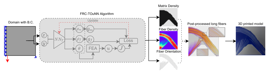
FRCs can be designed using long (i.e., continuous) fibers or short fibers; the former is preferred in mission-critical applications due to their superior material properties, dimensional stability, and robustness in fiber orientation and bonding (74; 29). However, for long-fiber FRCs to be effective, the base matrix topology, the fiber-density (spacing between individual fibers), and the fiber-orientation must be optimized simultaneously (Figure 1) (53; 54; 55).
Topology optimization (TO) is a computational design tool widely used during the early stages of design to automatically generate high-performance lightweight parts. Various TO methods have been proposed for optimizing FRCs, based on different design parameters and formulations (20; 35; 36). The most popular approach is based on Solid Isotropic Material with Penalization (SIMP) (63), where a fictitious pseudo-density field is defined over the underlying discretization is used for design representation, analysis, and optimization. Although in most practical cases, involving isotropic materials, we want every element to be either solid or void to ensure manufacturability, the pseudo-density at an element is allowed to take intermediate values () during the optimization to ensure differentiability. It is well-established that an intermediate density value at a given point in the design ( i.e., macro-scale) exhibits the homogenized properties of a microstructure at a lower scale (3). For instance, the effective elastic modulus for an element with intermediate density and penalization factor is approximated as , where is the elastic modulus of the base material. In other words, instead of modeling the geometric features at a lower scale with elastic modulus , we use the homogenized value at the macro-scale to simplify the formulation and improve computational efficiency.
On the other hand, FRC structures are inherently multi-scale and the mesh-dependent representation of the matrix-topology and fiber layout can pose several limitations in the physical realization and manufacturing of the optimized part. To maintain computational efficiency, analysis and optimization are performed using homogenized properties defined by the “rule of mixture”. For instance, given the volume fraction of fibers and elastic moduli for fibers and matrix , we have:
| (1) |
To realize the fiber inclusions at a lower scale, the design representation must be able to accommodate sub-element geometric and material queries. However, a discretized representation of FRC structures, where the fiber orientations are associated with each finite element, is not suitable for extracting high-resolution continuous fibers while enforcing sub-element fiber spacing — to quote (20) “…element-wise fiber orientation is not amenable for manufacturing or 3D printing …”.
In this paper, we rely on a mesh-independent neural-network (NN) representation of the matrix-topology, fiber-density, and fiber-orientation. The implicit NN-based representation enables geometric and material queries at a higher resolution than the background mesh, which leads to accurate extraction of functionally-graded continuous fibers. Further, by integrating the physical simulations into the NN computational framework, we leverage automatic differentiation (AD) to provide end-to-end automated sensitivity analysis by extending the method presented in (15; 11) to continuous fiber reinforced composites. In other words, we eliminate the need to manually derive the sensitivity expressions and only need to define a loss function capturing the objective and constraints. This permits rapid exploration of material models and design objectives, especially for applications involving dynamic and nonlinear physics.
Figure 2 provides an overview of the proposed method, where the spatial coordinates from the Euclidean space are mapped to the frequency space. Thus, the design is implicitly represented by a fully-connected feedforward NN with its output layer comprising three neurons corresponding to the matrix-topology, fiber-density, and fiber-orientation. As the finite element analysis (FEA) is performed within an NN framework (e.g., PyTorch), we leverage AD to compute the sensitivities and update the NN weights (e.g., Adam optimizer). Once the NN is trained, i.e., once the optimization is complete, a high-resolution FRC can be extracted and fabricated, for instance, using additive manufacturing (AM).
2 Literature Review
2.1 FRC Optimization Methods
While analytical methods have been developed for optimizing FRCs (5; 17; 40), the most popular method for optimizing FRCs is through topology optimization (TO). Current TO methods include density based (3; 4; 64; 65), level-set (77), topological sensitivity (71; 43; 42), and evolutionary methods (61). Among these, the density based methods are the most popular.
Optimizing the matrix-topology using TO is fairly straightforward and is not discussed here (4). Instead, we consider TO methods for optimizing the fiber-density and fiber-orientation. These methods can be classified as (a) continuous fiber angle optimization (CFAO), (b) discrete material optimization (DMO), or (c) free material optimization (FMO). In CFAO, the orientation of the fiber in each element is treated as a continuous design variable (38; 80). For instance the simultaneous optimization of AM build orientation, topology and fiber orientation was reported (14), while the simultaneous optimization of the topology and oriented material microstructure was reported in (81). A common characteristics of these methods was that matrix at an element was either void, or present with oriented fibers. Recently, (36) proposed a full-scale method for simultaneous design of matrix topology and fiber orientation; however, the spacing was fixed. In contrast to these two-phase approaches (i.e., void and anisotropic material), a three-phase approach was proposed in (35) wherein fiber concentration was considered along with material fraction as design variables. A topological derivative based method was proposed in (20) with binary-valued fiber concentration at each point. In contrast to CFAO, DMO methods (69) restrict the orientation to predetermined discrete values. While DMO approaches are often simpler with better convergence, they may result in discontinuous fibers. Finally, in FMO, the individual components of the elasticity tensor are treated as design variables, leading to theoretically optimal designs, but may lack a physical interpretation (36).
2.2 FRC Post-Processing Methods
Once an optimal FRC is computed, a post-processing step is required to determine the fiber paths or layout. A commonly used approach is the streamline methodology where fiber paths are obtained from the streamlines of the optimized fiber angle field (31). However, this does not guarantee uniform fiber distribution, and thus could lead to sub-optimal overlaps or gaps in the structure. Another common approach used in level set methods is to use parallel offsets of the contours to generate the fibers (66). This, however, reduces the design freedom by requiring the fibers to orient along the contours of the structure and may lead to sub-optimal results. Recently, continuous fiber generation based on the stripe patterns algorithm proposed by (33) was used in (8) that allowed for the generation of continuous fibers, considering both orientation and concentration, without optimizing the distribution of the underlying matrix.
2.3 Application of Neural-Network in TO
Since the proposed method relies on NN for optimization, we review relevant literature. Applications of NN in TO can be classified under two categories: (a) accelerating TO through NN (b) directly using NN to compute topologies.
Under the former category, (84) proposed accelerating TO by predicting gradients via online training of a NN; (1) proposed training a convolutional NN with a large database of optimized topologies and their corresponding loads to speed up topology prediction under novel loading scenario. Similar strategies were proposed in (67) and (75). (47) proposed using a generative adversarial network to train a generator to predict topologies conditioned under different loading scenarios. (37) employed NN to recognize and replace evolving features, thereby reducing number of TO iterations. (78) and (76) trained autoencoders with data pertinent to homogenized microstructures. The encoders were then employed in a TO framework, thereby eliminating the need to perform homogenization during the optimization loop.
In contrast to training NNs with data, one can use them directly to capture the topology as implicit function of the spatial coordinates, by recognizing that NNs are nothing but functions capable of capturing complex signals. One approach is based on continuous coordinate networks whose representational capacity is limited by the network rather than the grid size. They have been recently employed for physics simulations (58), modeling 3D shapes (28), view synthesis (41), semantic labeling (34), texture synthesis (49) etc. Recently, coordinate NNs have been used for isotropic TO (10), (30). The current work extends this work for the optimization of FRCs.
2.4 Contributions and Outline
The proposed method can be classified as a CFAO method based on a neural-network representation to capture the matrix-topology, the fiber-orientation, and fiber-density. We summarize and contrast the capabilities of the proposed method against previous work in Table 2.
| Reference | Matrix Topology | Fiber Density | Fiber Orientation |
|---|---|---|---|
| (20), (14), (68), (9) | |||
| (35), (50) | |||
| (36), (70), (55) | |||
| Proposed |
The main contributions of this paper are:
- •
Introducing an implicit NN-based representation for FRCs that enables realization of continuous fibers at a high resolution.
- •
Expressing all computations including FEA in an end-to-end automatic differentiable framework for automated sensitivity analysis.
- •
Proposing a density-based TO approach by simultaneously optimizing all three design variables, while also reducing the number of design variables.
- •
Presenting a new post-processing method for extraction of continuous long fibers at a high resolution.
In Section 4, we describe the proposed optimization method and subsequent post-processing stage for continuous fiber extraction. In Section 5 we demonstrate the validity, robustness, and efficiency of the framework. Finally, research challenges, opportunities and conclusions are summarized in Section 6.
3 Literature Review
3.1 Topology Optimization of FRCs
As mentioned earlier, While analytical methods have been developed for optimizing FRCs (5; 17; 40), the most popular method for optimizing FRCs is through TO. Current TO methods include density-based (3), (4), (64; 65), level-set (77), topological sensitivity (71), (43) and evolutionary methods (61). Among these, the density-based methods are the most popular.
Optimizing the matrix topology using TO is fairly straightforward and is not discussed here(4). Instead, we consider TO methods for optimizing the fiber-density and fiber-orientation. These methods can be classified as (a) continuous fiber angle optimization (CFAO), (b) discrete material optimization (DMO), and (c) free material optimization (FMO).
In CFAO, the orientation of the fiber in each element is treated as a continuous design variable (38), (80). For instance, the simultaneous optimization of AM build orientation, topology and fiber orientation was reported (14). The simultaneous optimization of the topology and oriented material microstructure was reported in (81). A key factor was the models considered the matrix to be fully embedded with fibers. In other words, the topology either consisted of matrix fully embedded with oriented fibers or void. Recently, (36) proposed a full-scale method capable of simultaneous design for the topology, fiber path, and its morphology. However, the spacing was fixed throughout the design. In contrast to these two-phase approaches (i.e., void and anisotropic material), a three-phase approach was proposed in (35) wherein fiber concentration was considered along with material fraction in a given design space. A topological derivative based method was proposed in (20) with binary-valued fiber concentration at each point.
In contrast, DMO (69) restrict the orientation to predetermined discrete values. While DMO approaches are often simpler with better convergence, they may result in discontinuous fibers. However, a DMO model was used which limits the practicality of the design as discussed.
Finally, in FMO, the individual components of the elasticity tensor are treated as design variables, leading to theoretically optimal designs, but may lack a physical interpretation (36).
Once an optimal topology is computed with fiber orientations, a post-processing step is utilized to determine the fiber paths or layout. A commonly used approach is the streamline methodology where fiber paths are obtained from the streamlines of the optimized fiber angle field (31). However, this does not guarantee uniform fiber distribution and thus could lead to sub-optimal overlaps or gaps in the compiled structure. Another common approach with level set based topology optimization is to use the parallel offsets of the contours of the optimized structure to orient the fibers (66). This, however, reduces the design freedom by requiring the fibers to orient along the contours of the structure and may lead to sub-optimal results. Recently, continuous fiber compilation based on the stripe patterns algorithm proposed by (33) was used in (8) that allowed for the compilation of continuous fibers with consideration to orientation and concentration.
3.2 Neural-Network based TO
Since this paper exploits neural-networks (NNs) to carry out TO, we briefly review prior work in this discipline. Applications of NN in TO can be classified under three categories: (a) accelerating TO through NN, (b) TO via NN-generated input-topology maps, and (c) directly using NN to compute topologies. The first category includes the work of (1), (67), (75). Proposed methods under the second category include the works of (47), (82), (37), (22). Here, the generated topologies aren’t guaranteed to be valid. The third approach rely on the fact that NNs are but implicit functions capable of capturing complex topologies (30; 10).
3.3 Paper Contributions
The proposed method can be classified as a CFAO method. However, instead of assigning design variables to each element, we use a neural-network (NN) to capture the matrix topology, the fiber-orientation and fiber-density. The advantages of the proposed framework are: a) NN representation is smooth and differentiable over the domain, b) Expressing all computations in an end-end allows for automated sensitivity analysis c) one can extract continuous long fibers after optimization, d) the number of design variables is relatively small, and e) using a gradient based optimization, the three design variables can be simultaneously optimized.
4 Proposed Method
In this section, we discuss the proposed NN-based TO framework to optimize functionally graded FRC structures (FRC-TOuNN). Figure 3 illustrates the difference between the typical SIMP approach and the proposed method.
In a typical single-material SIMP (Figure 3(a)), the design is represented by the pseudo-density values at discrete finite elements . The same discretization is used for FEA to evaluate the field variable () and correspondingly the performance objective function (J) and other constraints (g). Given the analytical expressions for gradients with respect to the pseudo-density design variables, the elemental sensitivity values are computed. Then, by relying on the standard SIMP penalization technique (6), the density values are updated using gradient-based methods (e.g., optimality criteria (7) or method of moving asymptotes (72)).
This coupling of representations for analysis and design can pose limitations in the fidelity and accuracy of design features across different scales. Further, deriving the analytical expressions for sensitivity formulation can be tedious and challenging. The proposed FRC-TOuNN approach decouples the representation for design (NN weights) from that of FEA (discrete elements), which enables geometric queries at high resolution (e.g., fiber orientation) while leveraging the efficiency of FEA. In other words, the design variables (here comprising of matrix density, fiber density, and fiber orientation) are captured externally using a NN’s activation functions and weights and is independent of the underlying mesh. Thus, by relying on an appropriate material model (Section 4.4) and a loss function reflecting the objectives and constraints problem, the design is optimized using the NN’s built-in optimizer as depicted in Figure 3(b).
4.1 Design Variables
We will assume that a design domain with loads and restraints (boundary conditions) has been prescribed (for example, see Figure 1). The objective here is to simultaneously optimize the (matrix) topology, fiber density, and fiber orientation to minimize an objective while satisfying volume constraints on the matrix and fiber. To achieve this, we introduce three spatially varying variables: matrix density, , fiber density, , and orientation, . These are collectively represented as . The matrix density, , controls the overall topology, i.e., implies the matrix is absent, while implies the matrix is present. Intermediate densities will be discouraged through penalization as discussed later on. The fiber density, , controls the concentration fibers; intermediate values of the fiber density are permitted. While we theoretically allow for the presence of fibers even if the base matrix is absent, this will not occur in practice due to an imposed volume control on the fiber volume. Finally, the fiber orientation, , allows for continuously varying orientations of fibers.
4.2 Optimization Problem
To pose a valid FRC optimization problem, we impose two-volume constraints. First, we impose a desired matrix volume fraction via . This controls the overall topology of the design. Next, we control the fraction of this matrix that must be filled with fibers via . Consequently, one can pose the optimization problem as:
| (2a) | ||||||
| subject to | (2b) | |||||
| (2c) | ||||||
| (2d) | ||||||
| (2e) | ||||||
where is the design objective (compliance), and is the area of an element. Observe that with , the amount of fiber never exceeds the amount of base matrix. Further, under the optimal scenario, we expect the fiber density at a location to go to zero when the matrix density at that location goes to zero. No additional constraint is required/imposed.
4.3 Neural Network Representation
Typically, the design variables in FRC optimization are captured via an underlying mesh. However, in this work, for reasons stated earlier, the variables are represented via a fully connected feed-forward NN (27) (), The NN architecture is as follows (see Figure 4):
- 1.
Input Layer: The input to the NN are points within the domain.
- 2.
Fourier Embedding: The sampled points from the Euclidean input domain are first passed through a frequency space. As detailed in (73), (57) implicit coordinate-based NN’s perform poorly in capturing finer features. Following along (13), we incorporate a Fourier projection layer that acts as an approximate length scale filter. In addition, the projection helps in faster and stable convergence of the optimizer.
- 3.
Hidden Layers: The hidden layers consist of a series of Swish (, (59)) activated dense layers. To sufficiently demarcate the representation of the densities from the orientation, we introduce a fork in the hidden layers. In particular, we present two common layers, the outer layer interfacing with the Fourier projection layer. Further, the deeper common layer acts as an interface to two sub-layers with no interconnection among themselves. These two sub-layers individually connect to the densities and orientation outputs respectively.
- 4.
Output Layer: The output layer consists of three neurons corresponding to . The output layer is activated via a Sigmoid function to ensure the outputs are in the range . Further, the orientation is transformed as .
Thus the three design variables are now spatially varying and are controlled by the weights and bias of the NN. The weights and bias, denoted by the , now become the primary design variables, i.e., and so on. The strategy, therefore, is to optimize the matrix and fiber via the NN weights . Re-expressing the optimization problem in Equation 3 with the NN weights as design variables, we have,
| (3a) | ||||||
| subject to | (3b) | |||||
| (3c) | ||||||
| (3d) | ||||||
| (3e) | ||||||
4.4 Material Model
We now discuss the underlying material model. The matrix is characterized by its elastic modulus and Poisson’s ratio ; this yields the matrix elasticity tensor (16). The fiber is characterized by the elastic modulus along two axis , , Poisson’s ratio and shear modulus (assumed to be independent of Young’s modulus); this yields the fiber elasticity tensor (16), when the fiber is oriented along the -axis. Now given an arbitrary orientation , the fiber elasticity tensor is transformed as follows:
| (4) |
where and are the transformation matrices:
| (5) |
where and (the reader is referred to (16) for details). Note that the angle , and therefore, the transformation matrices are spatially varying, but the dependency on has been suppressed for readability. Finally, given a matrix density, , and a fiber density, , the effective elasticity tensor at any point can be expressed as:
| (6) |
As mentioned earlier, the matrix density, , is penalized using the SIMP penalty parameter to drive the design towards a topology. On the other hand, the fiber density, , is allowed to take intermediate values.
4.5 Finite Element Analysis
We will use conventional finite element analysis (FEA) as part of the optimization engine. Here, we use a structured quadrilateral mesh due to its simplicity (see Figure 3(b)).
One can now evaluate the element stiffness matrix as
| (7) |
where is the gradient of the shape matrix, and is the elasticity tensor evaluated at the center of the element. Since the elasticity tensor varies spatially, the element stiffness matrix must be computed for each element, and for each step of the optimization process. This can be computationally very expensive. We, therefore, exploit the concept of template stiffness matrices to reduce the computational effort.
Let
| (8) |
One can therefore express the stiffness matrix as follows
| (9) | ||||
where,
| (10) |
and
| (11) |
Observe that matrices need to be computed only once at the start of the optimization. Then, during optimization, the element stiffness matrices are computed efficiently via Equation 9, followed by the assembly of the global stiffness matrix . During each step of the optimization problem, we solve the structural problem
| (12) |
where is the imposed load, and is the displacement field.
4.6 Loss Function
NNs are designed to minimize an unconstrained function. We therefore convert the constrained optimization problem in Equation 3 to an unconstrained loss function via a simple penalty formulation (48):
| (13) |
where is the initial compliance, used here for scaling, and , are the penalty parameters. While they can vary independently, we treat them to be the same, i.e., in our experiments; please see Section 5 for additional details. The equality constraint Equation 3b is satisfied when solving for the displacement during FEA (Section 4.5) while box constraints of Equation 3e are satisfied automatically by the output of the NN (Section 4.3). The optimization scheme is illustrated in Figure 3(b).
4.7 Sensitivity Analysis
A critical ingredient for the update schemes during optimization is the sensitivity, i.e., derivative, of the loss function (Equation 13) with respect to the weights of the NN. Typically the sensitivity analysis is carried out manually. This can be laborious and error-prone, especially for non-trivial objectives. Here, by expressing all our computations including the FEA in PyTorch (52), we rely on the automatic differentiation (AD) capabilities of NNs to completely automate this step (15). AD performs a systematic derivation of the sensitivity using the chain-rule. We express the broader derivative terms in Equation 14. The forward and sensitivity computations are schematically depicted in Figure 5.
| (14) | ||||
4.8 Post Processing
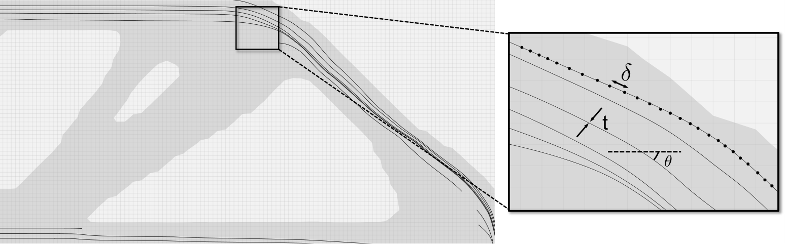
In this section, we address how one may interpret the output from the neural network post optimization to obtain continuous fiber tracks, where each track is represented by a set of ordered points. The global NN-representation allows us to query the relevant quantities at any location in the domain, i.e., . We assume that the fiber thickness () and step size () are specified. In the post processing algorithm below, we generate fibers and continuously update the fiber density to match the desired fiber-density as described below.
- 1.
is initialized to zero for all elements.
- 2.
We start at any non-void element where is less than the desired . If no such element exists, the post-processing algorithm stops.
- 3.
A fiber path is initiated at this element and is appended to a list; the quantity is updated for that element j (as the volume fraction of fiber within the element).
- 4.
Using the orientation and step-size at that element we take a step (in both directions, in two passes) to the next element.
- 5.
If: (a) the next element exists, and (b) is less than , we continue to along the path, else we terminate this fiber-path and continue to step-2.
For instance Figure 6 illustrates a few fibers extracted using the proposed post processing algorithm. Note that if the fiber thickness is much smaller than the element size, and if the desired fiber density is high, then multiple fibers can pass through an element.
4.9 Optimization Algorithm
The complete algorithm of the proposed framework is summarized in Algorithm 1, and schematically depicted in Figure 3(b).
5 Numerical Experiments
In this section, we conduct several experiments to illustrate the proposed framework. The implementation is in Python and uses the PyTorch library (52). The default parameters in the experiments are summarized in Table 3. Through the experiments, we investigate the following.
- 1.
Validation: We benchmark results obtained via our method against published results (20).
- 2.
Convergence Study: Typical convergence plots of the objective and volume constraints are reported and explained.
- 3.
Pareto Designs: Trade-off in performance when optimizing for varying volume fractions of the fiber and matrix is reported.
- 4.
Computational Cost: The cost to solve the optimization problem as a function of the number of elements used in FEA is studied. The cost division between the various components of the framework is summarized.
- 5.
Compliant Mechanism: By expressing our computations in an end-to-end differentiable form, we gain the ability to experiment with various objectives easily. We showcase this by designing compliant mechanisms.
- 6.
Multi-material: Fibrous composite structures often comprise regions made of different materials. We combine the present formulation with (12) to obtain structures with multi-material fibrous composites.
| Parameter | Description and default value |
|---|---|
| , | Isotropic matrix Young’s Modulus , Poisson’s ratio |
| , ,, |
Orthotropic fiber inclusion material constants.
, ,, |
| , | Allowed matrix volume fraction and fiber fraction |
| Number of frequencies in projection space = 150 | |
| and to allow wide range of length scales. | |
| , | Penalty method constraint with (, ) |
| SIMP penalty updated every iteration () | |
| lr | Adam Optimizer learning rate 0.01 |
| nelx, nely | Number of FEA mesh elements of (60, 30) along and respectively |
| h | Size of element along |
| Convergence criteria requiring a change in norm of the weights to be less than |
5.1 Validation
For validation, first, we replicate the FRC problem posed in (55) where only the fiber orientation of a beam loaded uniformly on its top edge (Figure 7) is to be optimized. We set . We compare the results obtained (Figure 7(c)) with the reported topologies in (55) (Figure 7(b)). We observe that the reported orientations are comparable. Figure 7(d) shows the post-processing result with continuous fibers and Figure 7(e) the 3D printed part. We note that the prints presented in this work are purely representative and additional manufacturing constraints may need to be imposed to render the parts manufacturable by current fiber printers.


As a second validation experiment, we consider the results presented in (20). where the matrix was not optimized, and the fiber is present or absent within the matrix, i.e., the concentration is either 1 or 0. The allowable fiber fraction was varied keeping and we compare the results with the proposed method and report the compliance and obtained topologies in Figure 8. We observe that the material gradation as obtained by the variable spacing/concentration of the fibers results in better designs with lower compliance values. The result obtained for was post processed to obtain long continuous fibers (with a representative fiber thickness of 0.1mm) as illustrated in Figure 9(a). For illustration thick fibers (1mm) were generated and printed using an UltiMaker 3 printer.


5.2 Convergence
In this example, we illustrate the typical convergence of the proposed algorithm using the symmetric half of the Michell structure Figure 10 with and . The compliance and the volume constraints of the matrix and fiber along with the matrix and fiber layout are illustrated at various instances in Figure 11. We observed a stable convergence using the simple penalty formulation.

5.3 Pareto Designs
An important consideration during the design stage is exploring the Pareto-front to make judicious engineering decisions. Towards this goal, we once again consider the problem in Figure 10 and explore the compliance and topology for varying values of and in Figure 12. As expected, we observe increasing compliance as we lower the allowed volume fractions.

5.4 Manufacturing Considerations
While one may obtain continuous fibers using the proposed algorithm, additional constraints may often be required to render the obtained designs manufacturable. For instance, the heavy clustering of fibers at the lower left in Figure 9(c) may not be actually manufacturable by continuous fiber printers. Further, the fibers may come infused/cladded with polymer matrix, making it possible to produce designs with only constant fiber density. Finally, there could be lower bounds on the fiber density owing to manufacturing limitations. Here we showcase how one may overcome these difficulties by imposing lower and upper bounds on the fiber density. In particular, the fiber density from the NN can further be transformed as , where and are the lower and upper bounds on the fiber density respectively. Figure 13 showcases the fiber densities with such imposed constraints. While we have outlined a few manufacturing constraints, other constraints may be imperative such as constraining the curvature of the fiber path, accessibility of the domain (44; 45; 46), distinction of shell and infill (79) substructures remain to be explored.


5.5 Computational Cost
We briefly summarize the computational costs with varying number of finite elements; all other parameters were kept constant at default values. We quantify the time taken for various operations in the optimization loop (1): namely, forward propagation (Algorithm 1.10), stiffness matrix assembly (Algorithm 1.11, Algorithm 1.12), sparse FEA solve (Algorithm 1.13 - Algorithm 1.17), backward propagation (Algorithm 1.18), and Adam optimizer (Algorithm 1.19). The computations are on a desktop machine with an Intel® Core™i7-7820X CPU with 8 processors running at 4.5 GHz, 32 GB of host memory, and an NVIDIA® GeForce® GTX 1080 GPU with 2,560 CUDA cores and 8 GB of device memory. The result summed over 200 iterations is summarized in Table 4. The time taken for individual operations on the CPU and GPU is illustrated in Figure 14(a) and Figure 14(b) respectively. We observe that the computational cost is dominated by backward-propagation. Note that the back-propagation is through the entire computation chain Figure 5. This includes one more solve of the FE system for the adjoint sensitivities as well as backprop through the NN. For a comparison of time taken by baseline TOuNN and mesh-based SIMP (64), we refer the readers to (10).
| #Elems | CPU Time (sec) | GPU Time (sec) |
|---|---|---|
| 200 | 2.695 | 1.701 |
| 800 | 10.092 | 4.779 |
| 1800 | 25.548 | 12.65 |
| 3200 | 52.848 | 28.943 |
| 5000 | 96.251 | 58.326 |
| 7200 | 168.898 | 115.881 |
5.6 Compliant Mechanism
While TO allows us to derive designs in an automated fashion for specified requirements, a key factor during the design stages is experimenting with the optimization objectives and constraints themselves. Current trends involve error-prone derivation and laborious implementation of the objectives and their sensitivities. In this work, by expressing our computations completely using an end-to-end differentiable framework. To illustrate, we consider the optimization of compliant mechanisms. Here, given input force , we are interested in maximizing the output displacement at stipulated nodes. By using automatic differentiation, one may simply change the objective in Equation 2a to Equation 15, without any other intervention
| (15) |
The setup and the design obtained with and is illustrated in Figure 15(a) and Figure 15(b) respectively.


5.7 Multi-Material Fibrous Composites
FRCs comprising for different materials are also of practical interest (24). Towards this, we extend our formulation to allow for multiple materials. In particular, we suppose one of the base matrix () to be fiber composites and others being a homogeneous matrix. Supposing there be different allowable matrix (and with being void), our topological description can be expressed as . Accordingly, the NN is modified to accommodate the new topological description (See Figure 16). Observe that only the output layer is modified to accommodate for the new description. The matrix output neurons are activated by a Softmax function to ensure physical validity of the densities via the partition of unity (Equation 16)
| (16) |
| (17) |
The effective Elasticity tensor at a point (Equation 4) can then be modified as:
| (18) | ||||
The modified optimization problem is expressed in Equation 19. We suppose the constituent materials to have a mass density . We then constrain the net mass of the system Equation 19c and the fiber volume fraction Equation 19d. For a detailed treatment of the multi-material formulation, we refer the readers to (12)
| (19a) | ||||||
| subject to | (19b) | |||||
| (19c) | ||||||
| (19d) | ||||||
| Material | Color Code | ||
|---|---|---|---|
| 1 | Black (matrix) | 0.6 | 0.4 |
| 2 | Blue | 4 | 1 |
| 3 | Gray (void) | 1e-9 | 1e-9 |
As an example, we consider the optimization of the tip-cantilever beam. We suppose that the domain can accommodate the materials in Table 5. The base matrix 1 may be impregnated with a fiber with , , and . With a net allowed mass of and fiber volume fraction , we obtain the optimized topology as shown in Figure 17.


6 Conclusion
The main contribution of this paper is a novel neural-network based topology optimization framework for optimizing continuous fiber reinforced composites. Representing the matrix density, fiber density and orientation implicitly via a NN, we showcased that one could extract long continuous fibers with sub-fiber spacing that reflects the fiber density. The method was validated by comparing it against published research, and characterized through several problems in 2D. The obtained designs were exported and printed on an Ultimaker 3 printer. Further, implementing an end-to-end differentiable framework allowed for faster experimentation. This was demonstrated by applying our framework to the design of compliance minimized design, design of compliant mechanism and multi-material FRCs. The extension of the proposed method to 3D to accommodate volumetric profiles (23), multi-axis prints (19) or build orientation (14) remains to be explored. Structurally validating the obtained results remains to be seen in the future (60). While long continuous fibers were obtained, no explicit measure constraining the length, continuity or curvature was imposed. Enforcing such constraints could be of practical importance (62). We observed that back-propagation consumes a large portion of the computational cost. Exploring techniques reducing this cost would be critical for wider adoption of the proposed method. While we used a direct sparse solver for FE simulation, large scale analysis would inevitably require iterative solver. Either integrating such solvers in automatic differentiation framework or online learning of FE solutions (18) and data-driven FE approaches (56) (2) remains to be explored. Future work will also focus on an improved post-processing algorithm.
Compliance with ethical standards
The authors declare that they have no conflict of interest.
References
- Banga et al. [2018a] Saurabh Banga, Harsh Gehani, Sanket Bhilare, Sagar Patel, and Levent Kara. 3D Topology Optimization using Convolutional Neural Networks. arXiv preprint arXiv:1808.07440, aug 2018a. URL http://arxiv.org/abs/1808.07440.
- Banga et al. [2018b] Saurabh Banga, Harsh Gehani, Sanket Bhilare, Sagar Patel, and Levent Kara. 3d topology optimization using convolutional neural networks. arXiv preprint arXiv:1808.07440, 2018b.
- Bendsoe and Sigmund [2003] M P Bendsoe and Ole. Sigmund. Topology optimization: theory, methods, and applications. Springer Berlin Heidelberg, 2 edition, 2003. ISBN 978-3-662-05086-6. doi:10.1063/1.3278595.
- Bendsoe et al. [2008] M. P. Bendsoe, J. M. Guedes, R. B. Haber, P. Pedersen, and J. E. Taylor. An Analytical Model to Predict Optimal Material Properties in the Context of Optimal Structural Design. Journal of Applied Mechanics, 61(4):930, dec 2008. ISSN 00218936. doi:10.1115/1.2901581. URL http://appliedmechanics.asmedigitalcollection.asme.org/article.aspx?articleid=1411416.
- Bendsoe et al. [1994] Martin P Bendsoe, JM Guedes, Robert B Haber, P Pedersen, and JE Taylor. An analytical model to predict optimal material properties in the context of optimal structural design. 1994.
- Bendsoe and Sigmund [2013] Martin Philip Bendsoe and Ole Sigmund. Topology optimization: theory, methods, and applications. Springer Science & Business Media, 2013.
- Berke and Khot [1987] L Berke and NS Khot. Structural optimization using optimality criteria. In Computer aided optimal design: structural and mechanical systems, pages 271–311. Springer, 1987.
- Boddeti et al. [2020] Narasimha Boddeti, Yunlong Tang, Kurt Maute, David W Rosen, and Martin L Dunn. Optimal design and manufacture of variable stiffness laminated continuous fiber reinforced composites. Scientific reports, 10(1):1–15, 2020.
- Brampton et al. [2015] Christopher J Brampton, K Chauncey Wu, and H Alicia Kim. New optimization method for steered fiber composites using the level set method. Structural and Multidisciplinary Optimization, 52(3):493–505, 2015.
- Chandrasekhar and Suresh [2020] Aaditya Chandrasekhar and Krishnan Suresh. TOuNN: Topology optimization using neural networks. Structural and Multidisciplinary Optimization, November 2020. doi:10.1007/s00158-020-02748-4.
- Chandrasekhar and Suresh [2021a] Aaditya Chandrasekhar and Krishnan Suresh. Multi-material topology optimization using neural networks. Computer-Aided Design, 136:103017, 2021a.
- Chandrasekhar and Suresh [2021b] Aaditya Chandrasekhar and Krishnan Suresh. Multi-material topology optimization using neural networks. Computer-Aided Design, 136:103017, 2021b.
- Chandrasekhar and Suresh [2022] Aaditya Chandrasekhar and Krishnan Suresh. Approximate length scale filter in topology optimization using fourier enhanced neural networks. Computer-Aided Design, page 103277, 2022.
- Chandrasekhar et al. [2020] Aaditya Chandrasekhar, Tej Kumar, and Krishnan Suresh. Build optimization of fiber-reinforced additively manufactured components. Structural and Multidisciplinary Optimization, 61(1):77–90, jan 2020. ISSN 16151488. doi:10.1007/s00158-019-02346-z. URL https://link.springer.com/article/10.1007/s00158-019-02346-z.
- Chandrasekhar et al. [2021] Aaditya Chandrasekhar, Saketh Sridhara, and Krishnan Suresh. Auto: a framework for automatic differentiation in topology optimization. Structural and Multidisciplinary Optimization, 64(6):4355–4365, 2021.
- Chawla [2012] Krishan K Chawla. Composite materials: science and engineering. Springer Science & Business Media, 2012.
- Cheng et al. [1994] HC Cheng, N Kikuchi, and ZD Ma. An improved approach for determining the optimal orientation of orthotropic material. Structural optimization, 8(2):101–112, 1994.
- Chi et al. [2021] Heng Chi, Yuyu Zhang, Tsz Ling Elaine Tang, Lucia Mirabella, Livio Dalloro, Le Song, and Glaucio H Paulino. Universal machine learning for topology optimization. Computer Methods in Applied Mechanics and Engineering, 375:112739, 2021.
- Dai et al. [2018] Chengkai Dai, Charlie CL Wang, Chenming Wu, Sylvain Lefebvre, Guoxin Fang, and Yong-Jin Liu. Support-free volume printing by multi-axis motion. ACM Transactions on Graphics (TOG), 37(4):1–14, 2018.
- Desai et al. [2021] Akshay Desai, Mihir Mogra, Saketh Sridhara, Kiran Kumar, Gundavarapu Sesha, and GK Ananthasuresh. Topological-derivative-based design of stiff fiber-reinforced structures with optimally oriented continuous fibers. Structural and Multidisciplinary Optimization, 63(2):703–720, 2021.
- Domm [2020] Matthias Domm. Printing of three-dimensional polymer composite structures with continuous fiber reinforcement. In Klaus Friedrich, Rolf Walter, Constantinos Soutis, Suresh G. Advani, and Ing. Habil. Bodo Fiedler, editors, Structure and Properties of Additive Manufactured Polymer Components, Woodhead Publishing Series in Composites Science and Engineering, pages 333–358. Woodhead Publishing, 2020. ISBN 978-0-12-819535-2. doi:https://doi.org/10.1016/B978-0-12-819535-2.00011-9. URL https://www.sciencedirect.com/science/article/pii/B9780128195352000119.
- Elingaard et al. [2021] Martin O Elingaard, Niels Aage, J Andreas Bærentzen, and Ole Sigmund. De-homogenization using convolutional neural networks. arXiv preprint arXiv:2105.04232, 2021.
- Ezair et al. [2018] Ben Ezair, Saul Fuhrmann, and Gershon Elber. Volumetric covering print-paths for additive manufacturing of 3D models. CAD Computer Aided Design, 100:1–13, 2018. ISSN 00104485. doi:10.1016/j.cad.2018.02.006. URL https://doi.org/10.1016/j.cad.2018.02.006.
- Galińska and Galiński [2020] Anna Galińska and Cezary Galiński. Mechanical joining of fibre reinforced polymer composites to metals—a review. part ii: riveting, clinching, non-adhesive form-locked joints, pin and loop joining. Polymers, 12(8):1681, 2020.
- Gandhi et al. [2020] Umesh Gandhi, Sebastian Goris, Tim A Osswald, and Yu-Yang Song. Discontinuous fiber-reinforced composites: fundamentals and applications. Carl Hanser Verlag GmbH Co KG, 2020.
- Glorot and Bengio [2010] Xavier Glorot and Yoshua Bengio. Understanding the difficulty of training deep feedforward neural networks. In Proceedings of the thirteenth international conference on artificial intelligence and statistics, pages 249–256, 2010.
- Goodfellow et al. [2016] Ian Goodfellow, Yoshua Bengio, and Aaron Courville. Deep Learning. MIT Press, 2016.
- Gropp et al. [2020] Amos Gropp, Lior Yariv, Niv Haim, Matan Atzmon, and Yaron Lipman. Implicit geometric regularization for learning shapes. arXiv preprint arXiv:2002.10099, 2020.
- Hine et al. [2002] Peter J Hine, Hans Rudolf Lusti, and Andrei A Gusev. Numerical simulation of the effects of volume fraction, aspect ratio and fibre length distribution on the elastic and thermoelastic properties of short fibre composites. Composites science and technology, 62(10-11):1445–1453, 2002.
- Hoyer et al. [2019] Stephan Hoyer, Jascha Sohl-Dickstein, and Sam Greydanus. Neural reparameterization improves structural optimization. arXiv preprint arXiv:1909.04240, 2019. URL https://arxiv.org/abs/1909.04240.
- Khani et al. [2015] A Khani, MM Abdalla, and Z Gürdal. Optimum tailoring of fibre-steered longitudinally stiffened cylinders. Composite Structures, 122:343–351, 2015.
- Kingma and Ba [2015] Diederik P. Kingma and Jimmy Lei Ba. Adam: A method for stochastic optimization. In 3rd International Conference on Learning Representations, ICLR 2015 - Conference Track Proceedings. International Conference on Learning Representations, ICLR, dec 2015.
- Knöppel et al. [2015] Felix Knöppel, Keenan Crane, Ulrich Pinkall, and Peter Schröder. Stripe patterns on surfaces. ACM Transactions on Graphics (TOG), 34(4):1–11, 2015.
- Kohli et al. [2020] Amit Pal Singh Kohli, Vincent Sitzmann, and Gordon Wetzstein. Semantic implicit neural scene representations with semi-supervised training. In 2020 International Conference on 3D Vision (3DV), pages 423–433. IEEE, 2020.
- Lee et al. [2018] Jaewook Lee, Dongjin Kim, Tsuyoshi Nomura, Ercan M Dede, and Jeonghoon Yoo. Topology optimization for continuous and discrete orientation design of functionally graded fiber-reinforced composite structures. Composite Structures, 201:217–233, 2018.
- Li et al. [2021] Hang Li, Liang Gao, Hao Li, Xiaopeng Li, and Haifeng Tong. Full-scale topology optimization for fiber-reinforced structures with continuous fiber paths. Computer Methods in Applied Mechanics and Engineering, 377:113668, 2021.
- Lin et al. [2018] Qiyin Lin, Jun Hong, Zheng Liu, Baotong Li, and Jihong Wang. Investigation into the topology optimization for conductive heat transfer based on deep learning approach. International Communications in Heat and Mass Transfer, 97:103–109, oct 2018. ISSN 07351933. doi:10.1016/j.icheatmasstransfer.2018.07.001.
- Lindgaard and Lund [2011] Esben Lindgaard and Erik Lund. Optimization formulations for the maximum nonlinear buckling load of composite structures. Structural and Multidisciplinary Optimization, 43(5):631–646, 2011.
- Liu et al. [2018] Jikai Liu, Andrew T Gaynor, Shikui Chen, Zhan Kang, Krishnan Suresh, Akihiro Takezawa, Lei Li, Junji Kato, Jinyuan Tang, Charlie CL Wang, et al. Current and future trends in topology optimization for additive manufacturing. Structural and Multidisciplinary Optimization, pages 1–27, 2018.
- Luo and Gea [1998] JH Luo and HC Gea. Optimal orientation of orthotropic materials using an energy based method. Structural optimization, 15(3-4):230–236, 1998.
- Mildenhall et al. [2020] Ben Mildenhall, Pratul P Srinivasan, Matthew Tancik, Jonathan T Barron, Ravi Ramamoorthi, and Ren Ng. Nerf: Representing scenes as neural radiance fields for view synthesis. arXiv preprint arXiv:2003.08934, 2020.
- Mirzendehdel and Suresh [2016] Amir M Mirzendehdel and Krishnan Suresh. Support structure constrained topology optimization for additive manufacturing. Computer-Aided Design, 81:1–13, 2016.
- Mirzendehdel et al. [2018] Amir M. Mirzendehdel, Behzad Rankouhi, and Krishnan Suresh. Strength-based topology optimization for anisotropic parts. Additive Manufacturing, 19:104–113, jan 2018. ISSN 22148604. doi:10.1016/j.addma.2017.11.007. URL https://www.sciencedirect.com/science/article/pii/S2214860416303475.
- Mirzendehdel et al. [2019] Amir M Mirzendehdel, Morad Behandish, and Saigopal Nelaturi. Exploring feasible design spaces for heterogeneous constraints. Computer-Aided Design, 115:323–347, 2019.
- Mirzendehdel et al. [2020] Amir M. Mirzendehdel, Morad Behandish, and Saigopal Nelaturi. Topology optimization with accessibility constraint for multi-axis machining. CAD Computer Aided Design, 122:102825, may 2020. ISSN 00104485. doi:10.1016/j.cad.2020.102825.
- Mirzendehdel et al. [2022] Amir M Mirzendehdel, Morad Behandish, and Saigopal Nelaturi. Topology optimization for manufacturing with accessible support structures. Computer-Aided Design, 142:103117, 2022.
- Nie et al. [2020] Zhenguo Nie, Tong Lin, Haoliang Jiang, and Levent Burak Kara. TopologyGAN: Topology Optimization Using Generative Adversarial Networks Based on Physical Fields Over the Initial Domain. arXiv preprint arXiv:2003.04685, mar 2020. URL http://arxiv.org/abs/2003.04685.
- Nocedal and Wright [2006] Jorge Nocedal and Stephen Wright. Numerical optimization. Springer Science & Business Media, 2006.
- Oechsle et al. [2019] Michael Oechsle, Lars Mescheder, Michael Niemeyer, Thilo Strauss, and Andreas Geiger. Texture fields: Learning texture representations in function space. In Proceedings of the IEEE/CVF International Conference on Computer Vision, pages 4531–4540, 2019.
- Papapetrou et al. [2020] Vasileios S Papapetrou, Chitrang Patel, and Ali Y Tamijani. Stiffness-based optimization framework for the topology and fiber paths of continuous fiber composites. Composites Part B: Engineering, 183:107681, 2020.
- Parandoush and Lin [2017] Pedram Parandoush and Dong Lin. A review on additive manufacturing of polymer-fiber composites. Composite Structures, 182:36–53, 2017.
- Paszke et al. [2019] Adam Paszke, Sam Gross, Francisco Massa, Adam Lerer, James Bradbury, Gregory Chanan, Trevor Killeen, Zeming Lin, Natalia Gimelshein, Luca Antiga, Alban Desmaison, Andreas Kopf, Edward Yang, Zachary DeVito, Martin Raison, Alykhan Tejani, Sasank Chilamkurthy, Benoit Steiner, Lu Fang, Junjie Bai, and Soumith Chintala. Pytorch: An imperative style, high-performance deep learning library. In Advances in Neural Information Processing Systems 32, pages 8024–8035. Curran Associates, Inc., 2019.
- Pedersen [1989] Pauli Pedersen. On optimal orientation of orthotropic materials. Structural optimization, 1(2):101–106, 1989.
- Pedersen [1990] Pauli Pedersen. Bounds on elastic energy in solids of orthotropic materials. Structural optimization, 2(1):55–63, 1990.
- Pedersen [1991] Pauli Pedersen. On thickness and orientational design with orthotropic materials. Structural Optimization, 3(2):69–78, 1991.
- Rade et al. [2021] Jaydeep Rade, Aditya Balu, Ethan Herron, Jay Pathak, Rishikesh Ranade, Soumik Sarkar, and Adarsh Krishnamurthy. Algorithmically-consistent deep learning frameworks for structural topology optimization. Engineering Applications of Artificial Intelligence, 106:104483, 2021.
- Rahaman et al. [2019] Nasim Rahaman, Aristide Baratin, Devansh Arpit, Felix Draxlcr, Min Lin, Fred A. Hamprecht, Yoshua Bengio, and Aaron Courville. On the spectral bias of neural networks. In 36th International Conference on Machine Learning, ICML 2019, volume 2019-June, pages 9230–9239, jun 2019. ISBN 9781510886988. URL http://arxiv.org/abs/1806.08734.
- Raissi et al. [2019] M. Raissi, P. Perdikaris, and G. E. Karniadakis. Physics-informed neural networks: A deep learning framework for solving forward and inverse problems involving nonlinear partial differential equations. Journal of Computational Physics, 378:686–707, feb 2019. ISSN 10902716. doi:10.1016/j.jcp.2018.10.045.
- Ramachandran et al. [2017] Prajit Ramachandran, Barret Zoph, and Quoc V Le. Searching for activation functions. arXiv preprint arXiv:1710.05941, 2017.
- Rankouhi et al. [2016] Behzad Rankouhi, Sina Javadpour, Fereidoon Delfanian, and Todd Letcher. Failure analysis and mechanical characterization of 3d printed abs with respect to layer thickness and orientation. Journal of Failure Analysis and Prevention, 16(3):467–481, 2016.
- Rozvany [2009] George IN Rozvany. A critical review of established methods of structural topology optimization. Structural and multidisciplinary optimization, 37(3):217–237, 2009.
- Shafighfard et al. [2019] Torkan Shafighfard, Eralp Demir, and Mehmet Yildiz. Design of fiber-reinforced variable-stiffness composites for different open-hole geometries with fiber continuity and curvature constraints. Composite Structures, 226:111280, 2019.
- Sigmund [1997] Ole Sigmund. On the design of compliant mechanisms using topology optimization. Journal of Structural Mechanics, 25(4):493–524, 1997.
- Sigmund [2001] Ole Sigmund. A 99 line topology optimization code written in matlab. Structural and multidisciplinary optimization, 21(2):120–127, 2001.
- Sigmund and Maute [2013] Ole Sigmund and Kurt Maute. Topology optimization approaches. Structural and Multidisciplinary Optimization, 48(6):1031–1055, 2013.
- Sivapuram et al. [2016] Raghavendra Sivapuram, Peter D. Dunning, and H. Alicia Kim. Simultaneous material and structural optimization by multiscale topology optimization. Structural and Multidisciplinary Optimization, 54(5):1267–1281, Nov 2016. ISSN 1615-147X. doi:10.1007/s00158-016-1519-x. URL http://link.springer.com/10.1007/s00158-016-1519-x.
- Sosnovik and Oseledets [2019] Ivan Sosnovik and Ivan Oseledets. Neural networks for topology optimization. Russian Journal of Numerical Analysis and Mathematical Modelling, 34(4):215–223, aug 2019. ISSN 15693988. doi:10.1515/rnam-2019-0018.
- Stegmann and Lund [2005a] J. Stegmann and E. Lund. Discrete material optimization of general composite shell structures. International Journal for Numerical Methods in Engineering, 62(14):2009–2027, Feb 2005a. ISSN 00295981. doi:10.1002/nme.1259. URL http://doi.wiley.com/10.1002/nme.1259.
- Stegmann and Lund [2005b] Jan Stegmann and Erik Lund. Discrete material optimization of general composite shell structures. International Journal for Numerical Methods in Engineering, 62(14):2009–2027, 2005b.
- Steuben et al. [2016] John C. Steuben, Athanasios P. Iliopoulos, and John G. Michopoulos. Implicit slicing for functionally tailored additive manufacturing. Computer-Aided Design, 77:107–119, aug 2016. ISSN 00104485. doi:10.1016/j.cad.2016.04.003. URL http://linkinghub.elsevier.com/retrieve/pii/S001044851630015X.
- Suresh [2013] Krishnan Suresh. Efficient generation of large-scale pareto-optimal topologies. Structural and Multidisciplinary Optimization, 47(1):49–61, jan 2013. ISSN 1615147X. doi:10.1007/s00158-012-0807-3. URL http://link.springer.com/10.1007/s00158-012-0807-3.
- Svanberg [1987] Krister Svanberg. The method of moving asymptotes—a new method for structural optimization. International journal for numerical methods in engineering, 24(2):359–373, 1987.
- Tancik et al. [2020] Matthew Tancik, Pratul P Srinivasan, Ben Mildenhall, Sara Fridovich-Keil, Nithin Raghavan, Utkarsh Singhal, Ravi Ramamoorthi, Jonathan T Barron, and Ren Ng. Fourier features let networks learn high frequency functions in low dimensional domains. arXiv preprint arXiv:2006.10739, 2020.
- Thomason [2002] JL Thomason. The influence of fibre length and concentration on the properties of glass fibre reinforced polypropylene: 5. injection moulded long and short fibre pp. Composites Part A: Applied Science and Manufacturing, 33(12):1641–1652, 2002.
- Ulu et al. [2016] Erva Ulu, Rusheng Zhang, and Levent Burak Kara. A data-driven investigation and estimation of optimal topologies under variable loading configurations. Computer Methods in Biomechanics and Biomedical Engineering: Imaging & Visualization, 4(2):61–72, 2016.
- Wang et al. [2020] Liwei Wang, Yu-Chin Chan, Faez Ahmed, Zhao Liu, Ping Zhu, and Wei Chen. Deep generative modeling for mechanistic-based learning and design of metamaterial systems. Computer Methods in Applied Mechanics and Engineering, 372:113377, 2020.
- Wang et al. [2003] Michael Yu Wang, Xiaoming Wang, and Dongming Guo. A level set method for structural topology optimization. Computer Methods in Applied Mechanics and Engineering, 192(1-2):227–246, jan 2003. ISSN 00457825. doi:10.1016/S0045-7825(02)00559-5. URL https://www.sciencedirect.com/science/article/pii/S0045782502005595.
- White et al. [2019] Daniel A White, William J Arrighi, Jun Kudo, and Seth E Watts. Multiscale topology optimization using neural network surrogate models. Computer Methods in Applied Mechanics and Engineering, 346:1118–1135, 2019.
- Wu et al. [2017] Jun Wu, Anders Clausen, and Ole Sigmund. Minimum compliance topology optimization of shell–infill composites for additive manufacturing. Computer Methods in Applied Mechanics and Engineering, 326:358–375, Nov 2017. ISSN 00457825. doi:10.1016/j.cma.2017.08.018. URL https://www.sciencedirect.com/science/article/pii/S0045782517305984.
- Xia and Shi [2017] Qi Xia and Tielin Shi. Optimization of composite structures with continuous spatial variation of fiber angle through shepard interpolation. Composite Structures, 182:273–282, 2017.
- Yan et al. [2019] Xiaolei Yan, Qiwang Xu, Dengfeng Huang, Yong Zhong, and Xiaodong Huang. Concurrent topology design of structures and materials with optimal material orientation. Composite Structures, 220:473–480, 2019.
- Yu et al. [2019] Yonggyun Yu, Taeil Hur, Jaeho Jung, and In Gwun Jang. Deep learning for determining a near-optimal topological design without any iteration. Structural and Multidisciplinary Optimization, 59(3):787–799, mar 2019. ISSN 16151488. doi:10.1007/s00158-018-2101-5.
- Zhang et al. [2017] Pu Zhang, Jikai Liu, and Albert C. To. Role of anisotropic properties on topology optimization of additive manufactured load bearing structures. Scripta Materialia, 135:148–152, Jul 2017. ISSN 13596462. doi:10.1016/j.scriptamat.2016.10.021. URL http://linkinghub.elsevier.com/retrieve/pii/S1359646216305164.
- Zhang et al. [2021] Yuyu Zhang, Heng Chi, Binghong Chen, Tsz Ling Elaine Tang, Lucia Mirabella, Le Song, and Glaucio H Paulino. Speeding up computational morphogenesis with online neural synthetic gradients. In 2021 International Joint Conference on Neural Networks (IJCNN), pages 1–8. IEEE, 2021.