Matings of cubic polynomials with a fixed critical point. Part II: $\alpha$-symmetry of limbs

For all $F_{a}\in\mathcal{H}_{0}$, the Julia set of $F_{a}$ is the simple closed curve $\partial U_{a}$ and $-a\in U_{a}$. Now suppose $F=F_{a}\in\mathcal{C}(\mathcal{S}_{1})\setminus\mathcal{H}_{0}$. Then, by Böttcher’s theorem, there exists a conformal isomorphism $\text{B\"{o}t}=\text{B\"{o}t}_{a}\colon U_{a}\to\mathbb{D}$ which satisfies

By a theorem of Roesch [16] (see also [8, 17]), $\partial U_{a}$ is a simple closed curve. Hence by Carathéodory’s Theorem, there exists a homeomorphic extension of Böt to the boundary $\partial U_{a}$. By abuse of notation, we will also use Böt for this homeomorphism from $\overline{U}_{a}$ to $\overline{\mathbb{D}}$. Thus for each point $z\in\partial U_{a}$, there exists a unique $t\in\mathbb{T}$ such that $z=\text{B\"{o}t}(e^{2\pi it})$. For brevity we will write $\beta(t)$ instead of $\text{B\"{o}t}(e^{2\pi it})$ and call $t$ the internal angle of $z$. The following theorem then describes the structure of the (filled) Julia set of a map in $\mathcal{C}(\mathcal{S}_{1})\setminus\mathcal{H}_{0}$.

We call $K_{t}$ a (dynamical) limb for the map $F$; the point $\beta(t)$ where $K_{t}$ meets $U_{a}$ is called the root point of the limb $K_{t}$. The set $K_{t_{0}}$ is called the critical limb of $F_{a}$.

Suppose a polynomial $F$ has a connected filled Julia set $K(F)$. By Böttcher’s theorem, there exists a conformal isomorphism $\text{B\"{o}t}_{F}\colon\widehat{\mathbb{C}}\setminus\overline{\mathbb{D}}\to\widehat{\mathbb{C}}\setminus K(F)$ which conjugates the map $z\mapsto z^{d}$ on $\widehat{\mathbb{C}}\setminus\overline{\mathbb{D}}$ to the map $F$ on $\widehat{\mathbb{C}}\setminus K(F)$. Furthermore, there is a unique choice of $\text{B\"{o}t}_{F}$ which is tangent to the identity at infinity.

We will often use the notation $R_{a}(t)$ instead of $R_{F_{a}}(t)$ for a polynomial $F_{a}\in\mathcal{S}_{1}$. If the choice of polynomial is clear, we sometimes drop the subscript altogether. By Carathéodory’s theorem, the filled Julia set $K(F)$ (or equivalently, the Julia set $J(F)$) of $F$ is locally connected if and only if $\text{B\"{o}t}_{F}$ extends continuously to the unit circle. The induced semiconjugacy $\gamma_{F}\colon\mathbb{R}/\mathbb{Z}\to J(F)$ is called the Carathéodory loop. The point $\gamma_{F}(t)\in J(F)$ is called the landing point of the ray $R_{F}(t)$ and a point $z$ of the Julia set is called biaccessible if it is the landing point of (at least) two external rays. That is, there exists $s\neq t$ such that $z=\gamma_{F}(s)=\gamma_{F}(t)$.

We will also need the notion of limbs in the parameter space. For a map $F_{a}\in\mathcal{H}_{0}$, then similarly to the above, there exists a unique conformal isomorphism Böt on a neighbourhood of $a$ conjugating $F_{a}$ to the map $w\mapsto w^{2}$. By Lemma 3.6 in [14], Böt can be analytically continued to a well-defined holomorphic function on a neighbourhood of the free critical point $-a$. We may then define a holomorphic function $\phi\colon\mathcal{H}_{0}\to\mathbb{D}$ by $\phi(a)=\text{B\"{o}t}_{a}(-a)$. This map $\phi$ then extends to a continuous map $\phi\colon\mathcal{C}(\mathcal{S}_{1})\to\overline{\mathbb{D}}$ such that if $F\in\mathcal{C}(\mathcal{S}_{1})\setminus\mathcal{H}_{0}$ then $\phi(F)=e^{2\pi it_{0}}$, where $t_{0}\in[0,1)$ is the internal argument of the critical limb of $F$.

Let $t_{0}\in(0,1)$. We define the (parameter) limb $\mathcal{L}_{t_{0}}^{+}$ to be the set

and analogously

We will show that one can distinguish $\mathcal{L}_{t_{0}}^{+}$ from $\mathcal{L}_{t_{0}}^{-}$ by dynamical means in Lemma 3.1. For $t_{0}=0$ we define $\mathcal{L}_{0}^{+}=\{F_{a}\in\mathcal{C}(\mathcal{S}_{1})\mid\phi(F)=e^{2\pi i0}\text{ and }\mathrm{Im}(a)<0\}$ and $\mathcal{L}_{0}^{-}=\{F_{a}\in\mathcal{C}(\mathcal{S}_{1})\mid\phi(F)=e^{2\pi i0}\text{ and }\mathrm{Im}(a)>0\}$. Note that by the $180^{\circ}$ rotational symmetry of $\mathcal{S}_{1}$, we have $F_{a}\in\mathcal{L}_{t_{0}}^{+}$ if and only if $F_{-a}\in\mathcal{L}_{t_{0}}^{-}$. The root point of a limb $\mathcal{L}_{t_{0}}^{\pm}$ is defined to be the unique point of $\mathcal{L}_{t_{0}}^{\pm}\cap\partial\mathcal{H}_{0}$.

In much of this paper, we will have to deal with the special case $t_{0}=0$ separately from other periodic internal arguments. Fortunately, most of the time the case for $t_{0}=0$ can be proved by inspection. When such a consideration is made, it will be clearly indicated.

We will also need the notion of parameter rays in the complement of the connectedness locus. They are closely related to the concept of external rays, as the following definition shows.

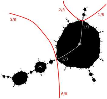
If $\theta$ is $m_{3}$-periodic, then the rays $\mathcal{R}(\theta-1/3)$ and $\mathcal{R}(\theta+1/3)$ land on a parabolic map. In this case the angles $\theta-1/3$ and $\theta+1/3$ are called co-periodic. The following properties of parameter limbs come from [14] (Compare also [4] for a more in-depth discussion). See Figure 1 for some examples of parameter limbs.

The above result implies the following.

In the case where $t_{0}$ is strictly preperiodic under $m_{2}$, the limb $\mathcal{L}_{t_{0}}^{\pm}$ consists of a single function $F_{a}\in\partial\mathcal{H}_{0}$, which is the landing point of exactly one parameter ray. Furthermore, it follows from Theorem 2.4 that for this map $F_{a}$, the root $\beta(t_{0})$ of the critical limb is the free critical point, and so the biaccessible points on $\partial U_{a}$ are $\beta(t_{0})$ and its preimages. In particular, $F_{a}$ has no biaccessible periodic points.

Let $f$ and $g$ be monic degree $d$ polynomials. We define

the complex plane compactified with the circle of directions at infinity. We then continuously extend the two polynomials to the circle at infinity by defining

Label this extended dynamical plane of $f$ (respectively $g$) by $\text{\textcopyright}_{f}$ (respectively $\text{\textcopyright}_{g}$). We create a topological $2$-sphere $\Sigma_{f,g}$ by gluing the two extended planes together along the circle at infinity:

where $\sim$ is the relation which identifies the point $\infty\cdot e^{2\pi it}\in\text{\textcopyright}_{f}$ with the point $\infty\cdot e^{-2\pi it}\in\text{\textcopyright}_{g}$. The formal mating is then defined to be the branched covering $f\uplus g\colon\Sigma_{f,g}\to\Sigma_{f,g}$ such that

A related concept to the formal mating is the topological mating. Let $f$ and $g$ be two monic degree $d$ polynomials with locally connected Julia set. First, construct the space $\Sigma_{f,g}$ as above, and define the ray-equivalence relation $\approx$ as follows. We denote by $\sim_{f}$ the smallest equivalence relation on $\text{\textcopyright}_{f}$ such that $x\sim_{f}y$ if and only if $x,y\in\overline{R}_{f}(t)$ for some $t$; the equivalence relation $\sim_{g}$ is defined analogously. Now $\approx$ is the smallest equivalence relation on $\Sigma_{f,g}$ which is generated by $\sim_{f}$ on $\text{\textcopyright}_{f}$ and $\sim_{g}$ on $\text{\textcopyright}_{g}$. The class $[x]$ of a point $x\in\Sigma_{f,g}$ will be called a ray-equivalence class.

Evidently, there is a surjection $K(f)\sqcup K(g)\to\Sigma_{f,g}/\approx$ given by the composition

Furthermore, since $x\approx y$ implies $(f\uplus g)(x)\approx(f\uplus g)(y)$, we can uniquely define the topological mating as the map $f\perp\!\!\!\perp g$ so that

commutes. Under favourable conditions, the topological space $\Sigma_{f,g}/\approx$ is a topological 2-sphere, in which case we say that $f$ and $g$ are topologically mateable. In fact, this occurs if and only if the equivalence relation $\approx$ is of Moore-type (see [12]). That is, $\approx$ is a non-trivial closed relation such that each equivalence class is closed and no equivalence class separates the sphere $\Sigma_{f,g}$.

Let $F\colon\Sigma\to\Sigma$ be an orientation-preserving branched self-covering of a topological $2$-sphere. We denote by $\Omega_{F}$ the critical set of $F$ and define

to be the postcritical set of $F$. We say that $F$ is postcritically finite if $|P_{F}|<\infty$. We call $F\colon\Sigma\to\Sigma$ a Thurston map if it is a postcritically finite orientation-preserving branched self-covering of a topological $2$-sphere.

If there exists an equivalence as above, we say that $F$ and $\widehat{F}$ are equivalent. Note that in particular, a postcritically finite rational map $R\colon\widehat{\mathbb{C}}\to\widehat{\mathbb{C}}$ on the Riemann sphere is a Thurston map. Hence it is natural to ask when a general Thurston map is equivalent to a rational map. In particular, since the formal mating of two postcritically finite polynomials is itself a Thurston map, we can ask if a given formal mating is equivalent to a rational map. This requires the notion of a Thurston obstruction, which we define below.

The importance of the above is due to the following rigidity theorem. A proof can be found in [6] or [11].

An $F$-stable multicurve with $\lambda(\Gamma)\geq 1$ is called a (Thurston) obstruction. The condition that $F$ has a hyperbolic orbifold is a purely combinatorial one; this condition can be checked by inspecting the dynamics on the union of the critical and postcritical sets of $F$. We remark that since the maps in this article have two fixed critical points, the respective orbifolds are guaranteed to be hyperbolic. For further details, see [6]. Following [20], we will say that a Thurston obstruction $\Gamma$ is irreducible if the associated matrix $F_{\Gamma}$ is irreducible. The following result from [20] (see also [21]) shows that it suffices to search for irreducible obstructions instead of Thurston obstructions.

In this paper, we will mainly be concerned with a special kind of obstruction: Levy cycles.

Note that a Levy cycle is an example of an irreducible obstruction. There is a close relationship between Levy cycles and periodic cycles of ray cycles, as given in the following theorem of Tan.

We remark that the converse of the corollary is not true: it is possible that two critical values belong to the same ray class but the mating is not obstructed, see Example 4.7. The following theorem from [18] indicates that all obstructions to matings of pairs of postcritically finite polynomials in $\mathcal{S}_{1}$ are topological.

Theorem 2.16 does not hold for general cubic polynomials: in [20], the authors constructed a mating of two postcritically finite cubic polynomials which was obstructed, but this obstruction was not a Levy cycle. Both the polynomials had critical points of period $3$.

Theorem 2.16 allows us to immediately prove the following.

We now discuss a technique due to Shishikura [19] (and also [20]) which allows us to modify a branched covering with removable Levy cycles so that it is no longer obstructed. This allows us to deal with cases where two polynomials are topologically mateable, but the formal mating has a Thurston obstruction.

Let $F$ be a Thurston map. We need to set up a partial ordering on the (possibly empty) set $\mathfrak{R}(F)$ of isotopy classes of removable Levy cycles for $F$. First, recall from Definition 2.13 that if $\Lambda$ is a removable Levy cycle, then the set $\Sigma\setminus\Lambda$ consists of $n$ disks $D_{1},\dotsc,D_{n}$ and an additional component $C$, such that for each $j$, the preimage $F^{-1}(D_{j})$ has a component $D_{j}^{\prime}$ isotopic to $D_{j-1}$ and the map $F\colon D_{j}^{\prime}\to D_{j}$ is a homeomorphism. Also, by definition, for each $k$, all components of $F^{-k}(D_{1})$ are disks. Define $\mathcal{D}(\Lambda)=\bigcup_{j=1}^{n}D_{j}$.

We now construct our partial order on $\mathfrak{R}(F)$. For two elements $\lambda_{1},\lambda_{2}\in\mathfrak{R}$, we say $\lambda_{1}<\lambda_{2}$ if there exists representatives $\Lambda_{1}$ and $\Lambda_{2}$ of $\lambda_{1}$ and $\lambda_{2}$ respectively such that $\mathcal{D}(\Lambda_{1})\subset\mathcal{D}(\Lambda_{2})$. Define $\mathfrak{R}^{\prime}$ to be the set of $\lambda\in\mathfrak{R}$ which are maximal under the partial order and such that for any Levy cycle $\Gamma$, the geometric intersection number $\lambda\cdot\Gamma=0$ (see e.g [7, p. 28] for the definition of geometric intersection number). In the case of matings, we have the following.

The above result allows us to define (essential) mateability of two polynomials $f$ and $g$ in $\mathcal{S}_{1}$. This adapts the definition of mateability given in [20] (Compare [19], where this was called the degenerate mating), which uses the notion of being weakly equivalent to a rational map. One can think of this weak equivalence as being obtained by shrinking (simultaneously) all removable Levy cycles of the branched covering $F=f\uplus g$ to points. If the original two polynomials were topologically mateable, then this new branched covering will no longer have any Levy cycles.

Since the matings of postcritically finite polynomials in $\mathcal{S}_{1}$ have hyperbolic orbifolds, the above definition is equivalent to the topological mating of $f$ and $g$ being Thurston equivalent to a rational map.

References

- [1] Krzysztof Barański. From Newton’s method to exotic basins. I. The parameter space. Fund. Math., 158(3):249–288, 1998.
- [2] Alexander Blokh, James M. Malaugh, John C. Mayer, Lex G. Oversteegen, and Daniel K. Parris. Rotational subsets of the circle under . Topology Appl., 153(10):1540–1570, 2006.
- [3] Araceli Bonifant, Xavier Buff, and John Milnor. Antipode preserving cubic maps: the fjord theorem. Proc. Lond. Math. Soc. (3), 116(3):670–728, 2018.
- [4] Araceli Bonifant and John Milnor. Cubic polynomial maps with periodic critical orbit, Part III: Tessellations. In preparation, 2022.
- [5] Bryan Boyd and Suzanne Boyd. Dynamics Explorer. Computer Software. https://sourceforge.net/projects/detool/.
- [6] Adrien Douady and John H. Hubbard. A proof of Thurston’s topological characterization of rational functions. Acta. Math., 171:263–297, 1993.
- [7] Benson Farb and Dan Margalit. A primer on mapping class groups, volume 49 of Princeton Mathematical Series. Princeton University Press, Princeton, NJ, 2012.
- [8] John Darroch Faught. Local connectivity in a family of cubic polynomials. PhD thesis, Cornell University, Ithaca, NY, 1992.
- [9] F. R. Gantmacher. The theory of matrices. Vol. 1. AMS Chelsea Publishing, Providence, RI, 1998.
- [10] Lisa R. Goldberg. Fixed points of polynomial maps. I. Rotation subsets of the circles. Ann. Sci. École Norm. Sup. (4), 25(6):679–685, 1992.
- [11] John Hamal Hubbard. Teichmüller theory and applications to geometry, topology, and dynamics. Vol. 2. Matrix Editions, Ithaca, NY, 2016. Surface homeomorphisms and rational functions.
- [12] Daniel Meyer and Carsten L. Petersen. On the notions of mating. Ann. Fac. Sci. Toulouse Math. (6), 21(5):839–876, 2012.
- [13] John W. Milnor. Dynamics in One Complex Variable. Princeton University Press, 3rd edition, 2006.
- [14] John W. Milnor. Cubic polynomial maps with periodic critical orbit. I. In Complex dynamics, pages 333–411. A K Peters, Wellesley, MA, 2009.
- [15] Carsten L. Petersen and Saeed Zakeri. On combinatorial types of periodic orbits of the map . Adv. Math., 361, 2020.
- [16] Pascale Roesch. Puzzles de Yoccoz pour les applications à allure rationnelle. Enseign. Math. (2), 45(1-2):133–168, 1999.
- [17] Pascale Roesch. Hyperbolic components of polynomials with a fixed critical point of maximal order. Ann. Sci. École Norm. Sup. (4), 40(6):901–949, 2007.
- [18] Thomas Sharland. Matings of cubic polynomials with a fixed critical point, Part I: Thurston obstructions. Conform. Geom. Dyn., 23:205–220, 2019.
- [19] Mitsuhiro Shishikura. On a theorem of M. Rees for matings of polynomials. In The Mandelbrot set, theme and variations, volume 274 of London Math. Soc. Lecture Note Ser., pages 289–305. Cambridge Univ. Press, Cambridge, 2000.
- [20] Mitsuhiro Shishikura and Tan Lei. A family of cubic rational maps and matings of cubic polynomials. Experimental Math., 9:29–53, 2000.
- [21] Tan Lei. Matings of quadratic polynomials. Ergodic Th. Dyn. Sys., 12:589–620, 1992.
- [22] Saeed Zakeri. Rotation sets and complex dynamics, volume 2214 of Lecture Notes in Mathematics. Springer, 2018.