\CTEXsetup

[format=]section

Multi-mode Tensor Train Factorization with Spatial-spectral Regularization for Remote Sensing Images Recovery

Gaohang Yu¹¹ 1 Department of Mathematics, Hangzhou Dianzi University, 310018, China. E-mail: maghyu@hdu.edu.cn Shaochun Wan¹¹footnotemark: 1 Liqun Qi²² 2 Department of Applied Mathematics, The Hong Kong Polytechnic University, Hung Hom, Kowloon, Hong Kong. E-mail: liqun.qi@polyu.edu.hk Yanwei Xu³³ 3 Huawei Theory Research Lab, Hong Kong, China. E-mail: xuyanwei1@huawei.com

Abstract: Tensor train (TT) factorization and corresponding TT rank, which can well express the low-rankness and mode correlations of higher-order tensors, have attracted much attention in recent years. However, TT factorization based methods are generally not sufficient to characterize low-rankness along each mode of third-order tensor. Inspired by this, we generalize the tensor train factorization to the mode-k tensor train factorization and introduce a corresponding multi-mode tensor train (MTT) rank. Then, we proposed a novel low-MTT-rank tensor completion model via multi-mode TT factorization and spatial-spectral smoothness regularization. To tackle the proposed model, we develop an efficient proximal alternating minimization (PAM) algorithm. Extensive numerical experiment results on visual data demonstrate that the proposed MTTD3R method outperforms compared methods in terms of visual and quantitative measures.
Key words: Multi-mode tensor train factorization; tensor completion; remote sensing images recovery

1 Introduction

With the rapid development of information technology, realistic data, such as remote sensing image, color image and video, tend to have high dimensions and complex structures. Tensor, as a high-dimensional generalization of vector and matrix, can better characterize the complex essential structures of higher-order data. Besides, higher-order tensors have extensive applications in many fields, such as multispectral image (MSI) recovery [1], hyperspectral image (HSI) restoration [2, 3, 4], image/video inpainting [4, 5, 6, 7, 8], and signal reconstruction [9].

Due to unacceptable cost of collecting complete data or loss of information during transmission, many real-world higher-order tensor data may contain missing entries. Therefore, tensor completion, which estimates the values of missing tensor entries, becomes one of the most important problems in tensor analysis and processing. Fortunately, many multi-dimensional tensors, such as color images and hyperspectral images (HSIs), are intrinsically or approximately low-rank and contain wealthy spatial-spectral information. As an extension of low-rank matrix completion (LRMC) [10], low-rank tensor completion (LRTC) utilizes the low-rank prior to express the relationship between the observed and missing entries, and can be mathematically written as:

	$\displaystyle\mathop{\min}\limits_{\mathcal{C}}$	$\displaystyle\mbox{rank}(\mathcal{C}),$		(1.1)
	$\displaystyle\mbox{s.t.}$	$\displaystyle{\displaystyle\mathcal{P}_{\Omega}}({\cal C}-{\cal M})=0,$		(1.1)

where $\mathcal{C}$ is the underlying tensor, $\mathcal{M}$ is the observed tensor, $\Omega$ is the index set for available entries, and $\mathcal{P}_{\Omega}(\cdot)$ is the projection operator that keeps the entries of $\mathcal{C}$ in $\Omega$ and zeros out others.

J. Liu et al. [5] generalized matrix trace norm to tensor case and proposed a tensor completion model based on the defined tensor trace norm:

	$\displaystyle\min_{\mathcal{X}}$	$\displaystyle\sum_{n=1}^{N}\alpha_{n}\\|C_{(n)}\\|_{\ast},$		(1.2)
	$\displaystyle\mbox{s.t.}$	$\displaystyle\mathcal{P}_{\Omega}(\mathcal{C})=\mathcal{P}_{\Omega}(\mathcal{M}).$		(1.2)

where $\alpha_{n}\geq 0$ and satisfies $\sum\nolimits_{n=1}^{N}\alpha_{n}=1$ , $C_{(n)}$ is the mode- $n$ unfolding matrix of $\mathcal{C}$ . Besides, three algorithms (SiLRTC, FaLRTC, HaLRTC) are developed to solve model (1.2). Then, N. Liu [11] et al. utilized the tensor trace norm as a convex surrogate for rank and proposed a low-rank tensor approximation (LRTA) model for hyperspectral and multispectral (HS-MS) fusion.

However, all these trace norm minimization methods involve the singular value decomposition (SVD) of $C_{(n)}$ and thus suffer from high computational cost. To tackle this issue, Xu et al. [4] utilized the matrix factorization method to preserve the low-rank structure of each mode matricization for efficiently handling large scale unfolding matrices:

	$\displaystyle\mathop{\min}\limits_{X,Y,\mathcal{C}}$	$\displaystyle\sum\limits_{n=1}^{N}{\dfrac{\alpha_{n}}{2}{{\left\\|{{X_{n}}{Y_{n}}-{C_{(n)}}}\right\\|}_{F}^{2}}},$		(1.3)
	$\displaystyle\mbox{s.t.}$	$\displaystyle{\displaystyle\mathcal{P}_{\Omega}}({\cal C}-{\cal M})=0,$		(1.3)

where $X=(X_{1},\ldots,X_{N})$ , $Y=(Y_{1},\ldots,Y_{N})$ , $\alpha_{n}$ are constants satisfying $\alpha_{n}\geq 0$ and $\sum\limits_{n=1}^{N}\alpha_{n}=1$ . The method, which is named as low-rank tensor completion by parallel matrix factorization (TMac), has shown better performance than FaLRTC. Many real-world data exhibits piecewise smooth prior, however, Xu et al. only consider the low-rank prior. Due to the ability of total variation (TV) to preserve edges[12], Ji et al. [13] considered to introduce it into the tensor completion problem (1.3).

	$\displaystyle\mathop{\min}\limits_{\mathcal{C},A,X}$	$\displaystyle\sum\limits_{n=1}^{N}{\dfrac{\alpha_{n}}{2}{{\left\\|{C_{(n)}-A_{n}X_{n}}\right\\|}_{F}^{2}}}+\mu\mbox{TV}(X_{3}),$		(1.4)
	$\displaystyle\mbox{s.t.}$	$\displaystyle{\displaystyle\mathcal{P}_{\Omega}}({\cal C}-{\cal M})=0,$		(1.4)

where $\mu$ is the regularization parameter, $A=(A_{1},\ldots,A_{N})$ , $X=(X_{1},\ldots,X_{N})$ , and $\mbox{TV}(X_{3})$ is the total variation of $X_{3}$ .

As pointed out by [14, 15], directly unfolding a tensor would destroy the original multi-way structure of the data, leading to vital information loss and degraded performance. Recently, on the basis of tensor-tensor product (t-product) and tensor singular value decomposition (t-SVD) [15, 16], Kilmer et al. [14] introduced the definitions of tensor multi-rank and tubal rank. Afterward, Semerci et al. [17] developed a new tensor nuclear norm (TNN) to better preserve the inherent low-rank structure of tensor. Then, Zhang et al. [7] proposed a TNN-based low-rank tensor completion model and applied it to video inpainting. It’s worth noting that TNN-based methods still involve computing t-SVD and thus time-consuming. Zhou et al. [6] proposed a low-tubal-rank tensor factorization model (TCTF) to avoid computing t-SVD, which factorizes the target tensor into the t-product of two smaller tensors:

	$\displaystyle\mathop{\min}\limits_{{\cal X},{\cal Y},{\cal C}}$	$\displaystyle\frac{1}{2}\left\\|{{\cal X}*{\cal Y}-{\cal C}}\right\\|_{F}^{2}$		(1.5)
	$\displaystyle\mbox{s.t.}$	$\displaystyle\cal{{\displaystyle P}_{\Omega}}({\cal C}-{\cal M})=0.$		(1.5)

In our recent work, we showed that the TCTF method lacks characterization of mode correlations. As pointed in [18, 19], tensor train (TT) factorization is especially suitable for high- dimensional tensors and can better characterize the global mode correlations. Thus, we proposed a streaming tensor completion method TTD2R on the basis of tensor train factorization and spatial-temporal constraint:

	$\displaystyle\mathop{\min}\limits_{{\cal C},{\cal X},{\cal Y},{\cal Z}}$	$\displaystyle\dfrac{1}{2}\left\\|{\cal C}-\llbracket{\cal X};{\cal Y};{\cal Z}\rrbracket\right\\|_{F}^{2}+\dfrac{\alpha_{1}}{2}\left\\|\mathcal{D}_{h}(\mathcal{C})\right\\|_{F}^{2}+\dfrac{\alpha_{2}}{2}\left\\|\mathcal{D}_{v}(\mathcal{C})\right\\|_{F}^{2},$		(1.6)
	$\displaystyle\mbox{s.t.}$	$\displaystyle P_{\Omega}(\mathcal{C})=P_{\Omega}(\mathcal{M}),$		(1.6)

where $\llbracket{\cal X};{\cal Y};{\cal Z}\rrbracket$ denotes TT factorization of $\mathcal{C}\in\mathbb{R}^{I_{1}\times I_{2}\times I_{3}}$ , $\mathcal{X},\mathcal{Y},\mathcal{Z}$ are TT cores, $\alpha_{1}$ and $\alpha_{2}$ are smoothness regularization parameters, $\mathcal{D}_{h}(\cdot)$ and $\mathcal{D}_{v}(\cdot)$ are first-order difference operators. TTD2R method outperforms other compared methods on color images inpainting and traffic data recovery, but it’s still not sufficient to express tensor data with low-rank property and smoothness along each mode.

In this paper, we define the mode-k tensor train factorization and MTT rank, which can more flexibly and accurately characterize low-rankness of HSIs, MSIs and gray videos. After that, we propose a novel low-rank tensor completion model for visual data recovery, which integrates MTT factorization with spatial-spectral smoothness.

The outline of this paper is as follows. Section 2 summarizes some notations, designs the mode-k tensor train factorization, and defines the multi-mode tensor train rank. Section 3 proposes a MTT factorization based third-order tensor completion model with spatial-spectral smoothness regularization terms, then a theoretically and numerically convergent PAM-based algorithm is developed to solve the problem. Section 5 evaluates the performance of the proposed method on color images, gray videos, MSIs, and remote sensing HSIs. Section 6 concludes this article.

2 Preliminaries

2.1 Notations

We denote vectors as bold lowercase letters (e.g., $\boldsymbol{a}$ ), matrices as uppercase letters (e.g., A), and tensors as calligraphic letters (e.g., $\mathcal{A}$ ). For a three-way tensor $\mathcal{A}\in\mathbb{R}^{I_{1}\times I_{2}\times I_{3}}$ , following the MATLAB notation, we denote its ( $i,j,s$ )th element as $\mathcal{A}(i,j,s)$ , its ( $i,j$ )th mode-1, mode-2, and mode-3 fibers as $\mathcal{A}(:,i,j)$ , $\mathcal{A}(i,:,j)$ , and $\mathcal{A}(i,j,:)$ , respectively. For the sake of clarity, we use $A_{1}^{(i)}\in\mathbb{R}^{I_{3}\times I_{2}}$ , $A_{2}^{(i)}\in\mathbb{R}^{I_{1}\times I_{3}}$ , and $A_{3}^{(i)}\in\mathbb{R}^{I_{2}\times I_{1}}$ to denote the $i$ th mode-1 (horizontal), mode-2 (lateral), and mode-3 (frontal) slices of $\mathcal{A}$ , respectively. The Frobenius norm of $\mathcal{A}$ is defined as $\|\mathcal{A}\|_{F}\coloneqq\sqrt{\sum_{i,j,s}|\mathcal{A}(i,j,s)|^{2}}$ . The $\ell_{1}$ norm of $\mathcal{A}$ is defined as $\|\mathcal{A}\|_{1}\coloneqq\sum_{i,j,s}|\mathcal{A}(i,j,s)|$ . Denote the mode- $k$ matricization of $\mathcal{A}$ as $A_{(k)}$ .

2.2 Multi-mode Tensor Train Factorization and Corresponding Ranks

Definition 2.1

(Tensor Mode- $k$ Permutation, refer to the definition in [3]): Given a three-way tensor $\mathcal{A}\in\mathbb{R}^{I_{1}\times I_{2}\times I_{3}}$ . The mode- $k$ permutation of $\mathcal{A}$ , denoted by $\vec{\mathcal{A}}^{k}$ , is defined as the tensor whose $i$ th mode- $2$ slice is the $i$ th mode- $k$ slice of $\mathcal{A}$ ., i.e., $\mathcal{A}(i,j,s)=\vec{\mathcal{A}}^{1}(s,i,j)=\vec{\mathcal{A}}^{2}(i,j,s)=\vec{\mathcal{A}}^{3}(j,s,i)$ . We define the corresponding operation as $\vec{\mathcal{A}}^{k}\coloneqq\text{permute}(\mathcal{A},k)$ and its inverse operation as $\mathcal{A}\coloneqq\text{ipermute}(\vec{\mathcal{A}}^{k},k)$ .

Refer to caption — Figure 1: Illustration of the mode- $k$ permutation for an $I_{1}\times I_{2}\times I_{3}$ tensor.

Figure 1 shows the mode- $k$ permutation of an $I_{1}\times I_{2}\times I_{3}$ tensor. With the above definitions, we design the mode- $k$ tensor train factorization of a third-order tensor.

Definition 2.2

(Mode- $k$ Tensor Train Factorization): The mode- $1$ tensor train (TT) factorization of $\mathcal{A}\in\mathbb{R}^{I_{1}\times I_{2}\times I_{3}}$ is defined as

\mathcal{A}(i_{1},i_{2},i_{3})=\mathcal{X}_{1}^{(i_{3})}\mathcal{Y}_{1}^{(i_{1})}\mathcal{Z}_{1}^{(i_{2})}

where $\mathcal{X}_{1}\in\mathbb{R}^{I_{3}\times r_{1}^{1}\times 1}$ , $\mathcal{Y}_{1}\in\mathbb{R}^{I_{1}\times r_{2}^{1}\times r_{1}^{1}}$ , $\mathcal{Z}_{1}\in\mathbb{R}^{I_{2}\times 1\times r_{2}^{1}}$ , $(r_{1}^{1},r_{2}^{1})\coloneqq(\mbox{rank}(A_{(3)}),\mbox{rank}(A_{(2)}))$ is the mode- $1$ TT rank of $\mathcal{A}$ . Denote the mode-1 TT factorization by $\mathcal{A}=\llbracket\mathcal{X}_{1};\mathcal{Y}_{1};\mathcal{Z}_{1}\rrbracket_{1}$ for brevity.

The mode- $2$ TT factorization of $\mathcal{A}\in\mathbb{R}^{I_{1}\times I_{2}\times I_{3}}$ is defined as

\mathcal{A}(i_{1},i_{2},i_{3})=\mathcal{X}_{2}^{(i_{1})}\mathcal{Y}_{2}^{(i_{2})}\mathcal{Z}_{2}^{(i_{3})}

where $\mathcal{X}_{2}\in\mathbb{R}^{1\times I_{1}\times r_{1}^{2}}$ , $\mathcal{Y}_{2}\in\mathbb{R}^{r_{1}^{2}\times I_{2}\times r_{2}^{2}}$ , $\mathcal{Z}_{2}\in\mathbb{R}^{r_{2}^{2}\times I_{3}\times 1}$ , $(r_{1}^{2},r_{2}^{2})\coloneqq(\mbox{rank}(A_{(1)}),\mbox{rank}(A_{(3)}))$ is the mode- $2$ TT rank of $\mathcal{A}$ . Denote it by $\mathcal{A}=\llbracket\mathcal{X}_{2};\mathcal{Y}_{2};\mathcal{Z}_{2}\rrbracket_{2}$ .

The mode- $3$ TT factorization of $\mathcal{A}\in\mathbb{R}^{I_{1}\times I_{2}\times I_{3}}$ is defined as

\mathcal{A}(i_{1},i_{2},i_{3})=\mathcal{X}_{3}^{(i_{2})}\mathcal{Y}_{3}^{(i_{3})}\mathcal{Z}_{3}^{(i_{1})}

where $\mathcal{X}_{3}\in\mathbb{R}^{r_{1}^{3}\times 1\times I_{2}}$ , $\mathcal{Y}_{3}\in\mathbb{R}^{r_{2}^{3}\times r_{1}^{3}\times I_{3}}$ , $\mathcal{Z}_{3}\in\mathbb{R}^{1\times r_{2}^{3}\times I_{1}}$ , $(r_{1}^{3},r_{2}^{3})\coloneqq(\mbox{rank}(A_{(2)}),\mbox{rank}(A_{(1)}))$ is the mode- $3$ TT rank of $\mathcal{A}$ . Denote it by $\mathcal{A}=\llbracket\mathcal{X}_{3};\mathcal{Y}_{3};\mathcal{Z}_{3}\rrbracket_{3}$ .

Actually, from above definitions, it’s easy to prove that $\mathcal{A}=\llbracket\mathcal{X}_{k};\mathcal{Y}_{k};\mathcal{Z}_{k}\rrbracket_{k}$ if and only if $\vec{\mathcal{A}}^{k}=\llbracket\vec{\mathcal{X}_{k}}^{k};\vec{\mathcal{Y}_{k}}^{k};\vec{\mathcal{Z}_{k}}^{k}\rrbracket_{2}$ . That is, the mode- $k$ TT ranks of $\mathcal{A}$ is equal to the mode-2 TT ranks of $\vec{\mathcal{A}}^{k}$ .

Definition 2.3

(Multi-mode Tensor Train Rank) The multi-mode tensor train (MTT) rank of a third-order tensor $\mathcal{A}\in\mathbb{R}^{I_{1}\times I_{2}\times I_{3}}$ , denoted as $\rm{rank}_{\rm{MTT}}(\mathcal{A})$ , is defined as a vector, whose $k$ th element is the mode- $k$ TT rank.

3 Tensor completion combining multi-mode tensor train factorization and spatial-spectral regularization

We establish the following low-rank tensor completion model by minimizing the MTT rank $\mbox{rank}_{\mbox{MTT}}(\cdot)$ of underlying tensor:

	$\displaystyle\min_{\mathcal{A}\in\mathbb{R}^{I_{1}\times I_{2}\times I_{3}}}$	$\displaystyle{\rm\displaystyle rank}_{MTT}(\mathcal{A})$		(3.1)
	$\displaystyle\mbox{s.t.}$	$\displaystyle P_{\Omega}(\mathcal{A})=P_{\Omega}(\mathcal{M})$		(3.1)

where $\mathcal{A}\in\mathbb{R}^{I_{1}\times I_{2}\times I_{3}}$ is the tensor to be filled; $\mathcal{M}$ is a normalized observed tensor such that $0\leq\mathcal{M}\leq 1$ .

In this paper, we utilize multi-mode tensor train factorization to flexibly characterize low-rankness along each mode of third-order tensor:

	$\displaystyle\mathop{\min}\limits_{{\cal A},{\cal X}_{u},{\cal Y}_{u},{\cal Z}_{u}}$	$\displaystyle\sum_{u=1}^{3}\frac{\alpha_{u}}{2}\left\\|{{\cal A}-\llbracket{\cal X}_{u};{\cal Y}_{u};{\cal Z}_{u}}\rrbracket_{u}\right\\|_{F}^{2},$		(3.2)
	$\displaystyle\mbox{s.t.}$	$\displaystyle P_{\Omega}(\mathcal{A})=P_{\Omega}(\mathcal{M}),$		(3.2)

where $\mathcal{X}_{u}$ , $\mathcal{Y}_{u}$ , $\mathcal{Z}_{u}$ are cores of the mode- $u$ TT factorization of $\mathcal{A}$ .

The low-MTT-rank constraint in (3.2) can be interpreted as a global feature, as it concerns the construction of the whole tensor. However, the low-rankness itself is generally not sufficient to recover the underlying data. As another significant prior, spatial-spectral smoothness appears in many real-world multi-dimensional data. To get better completion performance, we incorporate spatial-spectral regularization into (3.2) and obtain the improved version:

	$\displaystyle\mathop{\min}\limits_{{\cal A},{\cal X}_{u},{\cal Y}_{u},{\cal Z}_{u}}$	$\displaystyle\sum_{u=1}^{3}\frac{\alpha_{u}}{2}\left\\|{{\cal A}-\llbracket{\cal X}_{u};{\cal Y}_{u};{\cal Z}_{u}}\rrbracket_{u}\right\\|_{F}^{2}+\frac{\mu}{2}\\|\mathcal{D}_{w}(\mathcal{A})\\|_{F}^{2},$		(3.3)
	$\displaystyle\mbox{s.t.}$	$\displaystyle P_{\Omega}(\mathcal{A})=P_{\Omega}(\mathcal{M}),$		(3.3)

where $\mathcal{D}_{w}(\cdot)=\left[w_{1}\times\mathcal{D}_{h}(\cdot);w_{2}\times\mathcal{D}_{v}(\cdot);w_{3}\times\mathcal{D}_{t}(\cdot)\right]$ is the so-called weighted three-dimensional difference operator [20, 21] and $\mathcal{D}_{h}(\cdot)$ , $\mathcal{D}_{v}(\cdot)$ , $\mathcal{D}_{t}(\cdot)$ are the first-order difference operators with respect to three different directions of the tensor cube.

\mathcal{D}_{h}(\mathcal{A}(i,j,s))=\begin{cases}\mathcal{A}(i+1,j,s)-\mathcal{A}(i,j,s)&\mbox{if $i\neq I_{1}$}\\ \mathcal{A}(1,j,s)-\mathcal{A}(i,j,s)&\mbox{if $i=I_{1}$}\end{cases}

\mathcal{D}_{v}(\mathcal{A}(i,j,s))=\begin{cases}\mathcal{A}(i,j+1,s)-\mathcal{A}(i,j,s)&\mbox{if $i\neq I_{2}$}\\ \mathcal{A}(i,1,s)-\mathcal{A}(i,j,s)&\mbox{if $i=I_{2}$}\end{cases}

\mathcal{D}_{t}(\mathcal{A}(i,j,s))=\begin{cases}\mathcal{A}(i,j,s+1)-\mathcal{A}(i,j,s)&\mbox{if $i\neq I_{3}$}\\ \mathcal{A}(i,j,1)-\mathcal{A}(i,j,s)&\mbox{if $i=I_{3}$}\end{cases}

Moreover, problem (3.3) can be rewritten as

\mathop{\min}\limits_{{\cal A},{\cal X}_{u},{\cal Y}_{u},{\cal Z}_{u}}\quad f(\mathcal{X}_{u},\mathcal{Y}_{u},\mathcal{Z}_{u},\mathcal{A})

(3.4)

where

f(\mathcal{X}_{u},\mathcal{Y}_{u},\mathcal{Z}_{u},\mathcal{A})=f_{1}(\mathcal{X}_{1},\mathcal{Y}_{1},\mathcal{Z}_{1},\mathcal{A})+f_{2}(\mathcal{X}_{2},\mathcal{Y}_{2},\mathcal{Z}_{2},\mathcal{A})+f_{3}(\mathcal{X}_{3},\mathcal{Y}_{3},\mathcal{Z}_{3},\mathcal{A})+g(\mathcal{A})+\delta_{S}(\mathcal{A}),

f_{1}(\mathcal{X}_{1},\mathcal{Y}_{1},\mathcal{Z}_{1},\mathcal{A})=\frac{\alpha_{1}}{2}\left\|{{\cal A}-\llbracket{\cal X}_{1};{\cal Y}_{1};{\cal Z}_{1}}\rrbracket_{1}\right\|_{F}^{2},

f_{2}(\mathcal{X}_{2},\mathcal{Y}_{2},\mathcal{Z}_{2},\mathcal{A})=\frac{\alpha_{2}}{2}\left\|{{\cal A}-\llbracket{\cal X}_{2};{\cal Y}_{2};{\cal Z}_{2}}\rrbracket_{2}\right\|_{F}^{2},

f_{3}(\mathcal{X}_{3},\mathcal{Y}_{3},\mathcal{Z}_{3},\mathcal{A})=\frac{\alpha_{3}}{2}\left\|{{\cal A}-\llbracket{\cal X}_{3};{\cal Y}_{3};{\cal Z}_{3}}\rrbracket_{3}\right\|_{F}^{2},

g(\mathcal{A})=\frac{\mu}{2}\|\mathcal{D}_{w}(\mathcal{A})\|_{F}^{2},

S=\left\{\mathcal{W}\in\mathbb{R}^{I_{1}\times I_{2}\times I_{3}}\big|\mathcal{W}(i,j,k)=\mathcal{M}(i,j,k)\ \mbox{for}\ (i,j,k)\in\Omega;\ \mbox{while}\ \mathcal{W}(i,j,k)\in\left[0,1\right]\ \mbox{for}\ (i,j,k)\notin\Omega\right\},

\delta_{S}\left(\mathcal{A}\right)=\left\{\begin{array}[]{ll}0,&\mathcal{A}\in S;\\ +\infty,&\mathcal{A}\notin S.\end{array}\right.

4 Algorithm for solving (3.4)

4.1 Algorithm description

Model (3.4) is a multivariate optimization problem. Alternate Minimization(AM) algorithm is usually used to solve multivariate optimization problems due to its simplicity and efficiency. To improve the theoretical convergence and numerical stability of the AM algorithm, proximal terms are suggested to add in subproblems generated by AM algorithm[22, 23], which is called the Proximal Alternate Minimization (PAM) algorithm.

Given the initial point $(\mathcal{X}_{u,k},\mathcal{Y}_{u,k},\mathcal{Z}_{u,k},\mathcal{A}_{k})$ of the problem (3.4), the PAM iteration is defined as follows:

\mathcal{X}_{u,k+1}=\mathop{\arg\min}\limits_{\mathcal{X}_{u}}\ f_{u}({\cal X}_{u},{\cal Y}_{u,k},{\cal Z}_{u,k},{\cal A}_{k})+\frac{\rho}{2}\|\mathcal{X}_{u}-\mathcal{X}_{u,k}\|_{F}^{2},\ u\in\Xi(3),

(4.1)

\mathcal{Y}_{u,k+1}=\mathop{\arg\min}\limits_{\mathcal{Y}_{u}}\ f_{u}({\cal X}_{u,k+1},{\cal Y}_{u},{\cal Z}_{u,k},{\cal A}_{k})+\frac{\rho}{2}\|\mathcal{Y}_{u}-\mathcal{Y}_{u,k}\|_{F}^{2},\ u\in\Xi(3),

(4.2)

\mathcal{Z}_{u,k+1}=\mathop{\arg\min}\limits_{\mathcal{Z}_{u}}\ f_{u}({\cal X}_{u,k+1},{\cal Y}_{u,k+1},{\cal Z}_{u},{\cal A}_{k})+\frac{\rho}{2}\|\mathcal{Z}_{u}-\mathcal{Z}_{u,k}\|_{F}^{2},\ u\in\Xi(3),

(4.3)

\mathcal{A}_{k+1}=\mathop{\arg\min}\limits_{\mathcal{A}}\ f(\boldsymbol{x}_{k+1},\boldsymbol{y}_{k+1},\boldsymbol{z}_{k+1},{\cal A})+\frac{\rho}{2}\|\mathcal{A}-\mathcal{A}_{k}\|_{F}^{2},

(4.4)

where $\boldsymbol{x}_{k+1}=({\cal X}_{1,k+1};{\cal X}_{2,k+1};{\cal X}_{3,k+1})$ , $\boldsymbol{y}_{k+1}=({\cal Y}_{1,k+1};{\cal Y}_{2,k+1};{\cal Y}_{3,k+1})$ , $\boldsymbol{z}_{k+1}=({\cal Z}_{1,k+1};{\cal Z}_{2,k+1};{\cal Z}_{3,k+1})$ , $\rho>0$ is the given parameter.

It is obvious that (4.1)-(4.4) are all strongly convex optimization problems, whose existence and uniqueness are guaranteed. In Subsection 4.2, efficient methods will be introduced to solve (4.1)-(4.4).

4.2 Algorithm Implementation

In this section, we will concentrate on solving subproblems (4.1)-(4.4) arising from the PAM algorithm.

Firstly, it is easy to check that (4.1) and (4.3) have an unique closed-form solution respectively as follows:

{X}_{u,k+1}=\bigg[\rho I+\alpha_{u}\sum_{i=1}^{I_{u}}(Y_{u,k}^{(i)}Z_{u,k})(Y_{u,k}^{(i)}Z_{u,k})^{T}\bigg]{\bigg[\rho X_{u,k}+\alpha_{u}\sum_{i=1}^{I_{u}}{A_{u,k+1}^{(i)}(Y_{u,k}^{(i)}Z_{u,k})^{T}}\bigg]^{\dagger}},u\in\Xi(3),

(4.5)

{Z}_{u,k+1}=\bigg[\rho I+\alpha_{u}\sum_{i=1}^{I_{u}}(X_{u,k+1}Y_{u,k+1}^{(i)})^{T}(X_{u,k+1}Y_{u,k+1}^{(i)})\bigg]^{\dagger}{\bigg[\rho Z_{u,k}+\alpha_{u}\sum_{i=1}^{I_{u}}{(X_{u,k+1}Y_{u,k}^{(i)})^{T}}A_{u,k+1}^{(i)}\bigg]},u\in\Xi(3),

(4.6)

It’s clear that (4.2) and (4.4) are both strictly convex optimization problems with strongly convex objective function, which possess global and unique minimizers.

(4.2) is equivalent to the following unconstrained problem

Y_{u,k+1}^{(i)}=\mathop{\arg\min}\limits_{Y_{u}^{(i)}}\dfrac{1}{2}\|A_{u,k+1}^{(i)}-X_{u,k+1}Y_{u}^{(i)}Z_{u,k}\|_{F}^{2}+\frac{\rho}{2}\left\|Y_{u}^{(i)}-Y_{u,k}^{(i)}\right\|_{F}^{2},i\in\Xi(I_{u})

(4.7)

Treating $Y_{u}^{(i)}$ as variable of the objective function in the above problem, it’s then easy to check that the unique solution of the above problem is actually the solution of the following matrix equation

\alpha_{u}X_{u,k+1}^{T}X_{u,k+1}Y_{u}^{(i)}Z_{u,k}Z_{u,k}^{T}+\rho Y_{u}^{(i)}=\Gamma^{(i)}

(4.8)

where $\Gamma^{(i)}=\alpha_{u}X_{u,k+1}^{T}A_{u,k+1}^{(i)}Z_{u,k}^{T}+\rho Y_{u,k}^{(i)}$ . Notice that $X_{u,k+1}^{T}X_{u,k+1}$ and $Z_{u,k}Z_{u,k}^{T}$ are symmetric matrices, then there exist orthogonal matrices $Q_{1}$ and $Q_{2}$ , such that $X_{u,k+1}^{T}X_{u,k+1}=Q_{1}\Lambda_{1}Q_{1}^{T}$ and $Z_{u,k}Z_{u,k}^{T}=Q_{2}\Lambda_{2}Q_{2}^{T}$ , where $\Lambda_{1}$ and $\Lambda_{2}$ are diagonal matrices whose diagonal elements are eigenvalues of $X_{u,k+1}^{T}X_{u,k+1}$ and $Z_{u,k}Z_{u,k}^{T}$ , respectively. Multiplying $Q_{1}^{T}$ from the left and multiplying $Q_{2}$ from the right on both sides of (4.8), we can get

\alpha_{u}\Lambda_{1}\hat{Y}_{u}^{(i)}\Lambda_{2}+\rho\hat{Y}_{u}^{(i)}=\hat{\Gamma}^{(i)}

(4.9)

where $\hat{Y}_{u}^{(i)}=Q_{1}^{T}Y_{u}^{(i)}Q_{2}$ , $\hat{\Gamma}^{(i)}=Q_{1}^{T}\Gamma^{(i)}Q_{2}$ . Since $\Lambda_{1}$ and $\Lambda_{2}$ are both diagonal matrices, $\hat{Y}_{u}^{(i)}$ can be fast solved by

\hat{Y}_{u}^{(i)}(m,n)=\dfrac{\hat{\Gamma}^{(i)}(m,n)}{\rho+\alpha_{u}\Lambda_{1}(m)\Lambda_{2}(n)}.

(4.10)

Hense, $Y_{u,k+1}^{(i)}$ in (4.7) can be solved by

Y_{u}^{(i)}=Q_{1}\hat{Y}_{u}^{(i)}Q_{2}^{T}.

(4.11)

Note that

\begin{split}&\quad\sum_{u=1}^{3}\alpha_{u}\|{\cal A}-\llbracket{\cal X}_{u};{\cal Y}_{u};{\cal Z}_{u}\rrbracket_{u}\|_{F}^{2}\\ &=\sum_{u=1}^{3}\alpha_{u}\left\langle{\cal A}-\llbracket{\cal X}_{u};{\cal Y}_{u};{\cal Z}_{u}\rrbracket_{u},{\cal A}-\llbracket{\cal X}_{u};{\cal Y}_{u};{\cal Z}_{u}\rrbracket_{u}\right\rangle\\ &=\sum_{u=1}^{3}\alpha_{u}\left\langle\mathcal{A},\mathcal{A}\right\rangle-2\sum_{u=1}^{3}\alpha_{u}\left\langle\mathcal{A},\llbracket{\cal X}_{u};{\cal Y}_{u};{\cal Z}_{u}\rrbracket_{u}\right\rangle+\sum_{u=1}^{3}\alpha_{u}\left\langle\llbracket{\cal X}_{u};{\cal Y}_{u};{\cal Z}_{u}\rrbracket_{u},\llbracket{\cal X}_{u};{\cal Y}_{u};{\cal Z}_{u}\rrbracket_{u}\right\rangle\\ &=\left\langle\mathcal{A},\mathcal{A}\right\rangle-2\left\langle\mathcal{A},\sum_{u=1}^{3}\alpha_{u}\llbracket{\cal X}_{u};{\cal Y}_{u};{\cal Z}_{u}\rrbracket_{u}\right\rangle+\sum_{u=1}^{3}\alpha_{u}\|\llbracket{\cal X}_{u};{\cal Y}_{u};{\cal Z}_{u}\rrbracket_{u}\|_{F}^{2}\\ &=\left\langle\mathcal{A}-\sum_{u=1}^{3}\alpha_{u}\llbracket{\cal X}_{u};{\cal Y}_{u};{\cal Z}_{u}\rrbracket_{u},\mathcal{A}-\sum_{u=1}^{3}\alpha_{u}\llbracket{\cal X}_{u};{\cal Y}_{u};{\cal Z}_{u}\rrbracket_{u}\right\rangle+\sum_{u=1}^{3}\alpha_{u}\|\llbracket{\cal X}_{u};{\cal Y}_{u};{\cal Z}_{u}\rrbracket_{u}\|_{F}^{2}-\|\sum_{u=1}^{3}\alpha_{u}\llbracket{\cal X}_{u};{\cal Y}_{u};{\cal Z}_{u}\rrbracket_{u}\|_{F}^{2}\\ &=\|\mathcal{A}-\sum_{u=1}^{3}\alpha_{u}\llbracket{\cal X}_{u};{\cal Y}_{u};{\cal Z}_{u}\rrbracket_{u}\|_{F}^{2}+\sum_{u=1}^{3}\alpha_{u}\|\llbracket{\cal X}_{u};{\cal Y}_{u};{\cal Z}_{u}\rrbracket_{u}\|_{F}^{2}-\|\sum_{u=1}^{3}\alpha_{u}\llbracket{\cal X}_{u};{\cal Y}_{u};{\cal Z}_{u}\rrbracket_{u}\|_{F}^{2},\end{split}

(4.4) can be rewritten as

\mathcal{A}_{k+1}=\mathop{\arg\min}\limits_{\mathcal{A}}\frac{1}{2}\|\mathcal{A}-\sum_{u=1}^{3}\alpha_{u}\llbracket{\cal X}_{u,k};{\cal Y}_{u,k};{\cal Z}_{u,k}\rrbracket_{u}\|_{F}^{2}+\frac{\mu}{2}\|\mathcal{D}_{w}(\mathcal{A})\|_{F}^{2}+\frac{\rho}{2}\|\mathcal{A}-\mathcal{A}_{k}\|_{F}^{2}.

(4.12)

It can be solved by the following linear system:

\left[(1+\rho)I+\mu\mathcal{D}_{w}^{*}\mathcal{D}_{w}\right]\mathcal{A}=\sum_{u=1}^{3}\alpha_{u}\llbracket{\cal X}_{u,k};{\cal Y}_{u,k};{\cal Z}_{u,k}\rrbracket_{u}+\rho\mathcal{A}_{k},

(4.13)

where $\mathcal{D}_{w}^{*}$ denotes the adjoint operator of $\mathcal{D}_{w}$ . Finally, by the 3D Fourier transform (fftn) and its inverse transform (ifftn), we can obtained the closed-form solution

\tilde{\mathcal{A}}_{k+1}=\mbox{ifftn}\left(\dfrac{\mbox{fftn}(\sum_{u=1}^{3}\alpha_{u}\llbracket{\cal X}_{u,k};{\cal Y}_{u,k};{\cal Z}_{u,k}\rrbracket_{u}+\rho\mathcal{A}_{k})}{(1+\rho)\textbf{1}+\mu(\left|\mbox{fftn}(\mathcal{D}_{h})\right|^{2}+\left|\mbox{fftn}(\mathcal{D}_{v})\right|^{2}+\left|\mbox{fftn}(\mathcal{D}_{t})\right|^{2})}\right).

Therefore, $\mathcal{A}_{k+1}$ can be solved by

\mathcal{A}_{k+1}(i,j,s)=\left\{\begin{array}[]{ll}\min\{1,\max\{\tilde{\mathcal{A}}_{k+1}(i,j,s),0\}\},&(i,j,s)\notin\Omega,\\ \mathcal{M}(i,j,s),&(i,j,s)\in\Omega.\end{array}\right.

(4.14)

Algorithm 1 presents the PAM algorithm for solving (3.4).

Algorithm 1 The MTTD3R algorithm to solve (3.4)

Input: The observed data

\mathcal{M}\in\mathbb{R}^{I_{1}\times I_{2}\times I_{3}}

, index set

\Omega

Parameters: The initialized MTT ranks

(r_{1}^{u},r_{2}^{u})

\alpha_{u}

w

\mu\geq 0

\rho=5e-5

Initialize: Construct

{\cal X}_{u,0}

\mathcal{Y}_{u,0}

{\cal Z}_{u,0}

using TT-SVD[24] of

\vec{\mathcal{M}}^{u}

\epsilon=1e-6

, iteration N=500.

while

k\leq N

and not converged do

(1) Fix

{\cal X}_{u,k}

\mathcal{Y}_{u,k}

{\cal Z}_{u,k}

u\in\Xi(3)

to update

{\cal A}_{k+1}

via (4.14).

(2) Fix

{\cal A}_{k+1}

{\cal Y}_{u,k}

and

\mathcal{Z}_{u,k}

to update

{\cal X}_{u,k+1}

via (4.5).

(3) For every

n\in\Xi(I_{u})

, fix

{\cal A}_{k}^{(n)}

\mathcal{X}_{u,k+1}

and

\mathcal{Z}_{u,k}

to update

{\cal Y}_{u,k+1}^{(n)}

via (4.7).

(4) Fix

\mathcal{A}_{k+1}

\mathcal{X}_{u,k+1}

\mathcal{Y}_{u,k+1}

to update

{\cal Z}_{u,k+1}

via (4.6).

(5) Check the stopping criterion:

\frac{\|\mathcal{A}^{k+1}-\mathcal{A}^{k}\|_{F}^{2}}{\|\mathcal{A}^{k+1}\|_{F}^{2}}\leq\epsilon

end while

Output : Recovered tensor

\mathcal{A}^{k+1}

4.3 Convergence analysis

In this section, we will prove the global convergence of Algorithm 1. For convenience, we rewrite the objective function (3.4) as

f(\boldsymbol{x},\boldsymbol{y},\boldsymbol{z},\mathcal{A})=h(\boldsymbol{x},\boldsymbol{y},\boldsymbol{z},\mathcal{A})+g(\mathcal{A})+\delta_{S}(\mathcal{A}),

(4.15)

where $\boldsymbol{x}=({\cal X}_{1};{\cal X}_{2};{\cal X}_{3})$ , $\boldsymbol{y}=({\cal Y}_{1};{\cal Y}_{2};{\cal Y}_{3})$ , $\boldsymbol{z}=({\cal Z}_{1};{\cal Z}_{2};{\cal Z}_{3})$ , $h=f_{1}+f_{2}+f_{3}$ .

To show the convergence of PAM algorithm, the following convergence theory is needed.

Lemma 4.1

[25] Let $f:\mathbb{R}^{n}\rightarrow\mathbb{R}\cup\left\{+\infty\right\}$ be a PLSC function. Let $\left\{\boldsymbol{x}_{k}\right\}_{k\in\mathbb{N}}\subset\mathbb{R}^{n}$ be a sequence such that

H1

$\left(\mbox{Sufficient decrease condition}\right)$ For each $k\in\mathbb{N}$ , there exits $a\in\left(0,+\infty\right)$ such that $f\left(\boldsymbol{x}_{k+1}\right)+a\|\boldsymbol{x}_{k+1}-\boldsymbol{x}_{k}\|_{2}^{2}\leq f\left(\boldsymbol{x}_{k}\right)$ hold£»
H2

$\left(\mbox{Relative error condition}\right)$ For each $k\in\mathbb{N}$ , there exits $\boldsymbol{w}_{k+1}\in\partial f\left(\boldsymbol{x}_{k+1}\right)$ and a constant $b\in\left(0,+\infty\right)$ such that $\|\boldsymbol{w}_{k+1}\|_{2}\leq b\|\boldsymbol{x}_{k+1}-\boldsymbol{x}_{k}\|_{2}$ hold£»

$\left(\mbox{Continuity condition}\right)$ There exists a subsequence $\left\{\boldsymbol{x}_{k_{j}}\right\}_{j\in\mathbb{N}}$ and $\bar{\boldsymbol{x}}\in\mathbb{R}^{n}$ such that

\boldsymbol{x}_{k_{j}}\rightarrow\bar{\boldsymbol{x}}\mbox{ and }f\left(\boldsymbol{x}_{k_{j}}\right)\rightarrow f\left(\bar{\boldsymbol{x}}\right),j\rightarrow\infty.

If $f$ has the KŁ property at $\bar{\boldsymbol{x}}$ , then

(i)

$\boldsymbol{x}_{k}\rightarrow\bar{\boldsymbol{x}}$
(ii)

$\bar{\boldsymbol{x}}$ is a critical point of $f$ , i.e., $0\in\partial f\left(\bar{\boldsymbol{x}}\right)$ ;
(iii)

the sequence $\left\{\boldsymbol{x}_{k}\right\}_{k}\in\mathbb{N}$ has a finite length, i.e.,

$\sum_{k=0}^{+\infty}\|\boldsymbol{x}_{k+1}-\boldsymbol{x}_{k}\|_{2}<+\infty.$

Next, we show that the objective function $f$ in (4.15) and the sequence $\left(\boldsymbol{x}_{k},\boldsymbol{y}_{k},\boldsymbol{z}_{k},\mathcal{A}_{k}\right)$ generated by PAM algorithm satisfy the assumptions in Lemma 4.1. Hence, we establish the following convergence theorem.

Theorem 4.2

Assume that the sequence $\left(\boldsymbol{x}_{k},\boldsymbol{y}_{k},\boldsymbol{z}_{k},\mathcal{A}_{k}\right)$ generated by Algorithm 1 is bounded. Then, the algorithm can converge to a critical point of $f$ .

Proof. First, we need to prove that $f$ is a proper lower semi-continuous function. $S$ is a non-empty closed set, which means that $\delta_{S}(\cdot)$ is a proper lower semi-continuous (PLSC) function. Moreover, we can know that $h$ is a polynomial function with respect to $(\boldsymbol{x},\boldsymbol{y},\boldsymbol{z},\mathcal{A})$ by the definition of Frobenius norm. Then $h$ is semi-algebraic and thus a KŁ function (which is intrinsically PLSC)[25]. Similarly, $g$ is also lower semi-continuous and proper, so the function $f$ is proper semi-continuous function.

Second, it’s easy to see that Algorithm 1 is an example of algorithm (61)-(63) displayed in [25] with $B_{i}=\rho I$ . Thus, the sequence $\left(\boldsymbol{x}_{k},\boldsymbol{y}_{k},\boldsymbol{z}_{k},\mathcal{A}_{k}\right)$ generated by Algorithm 1 satisfy the conditions H1, H2, H3 in Lemma 4.1.

Third, we show that $f$ satisfies the KL property at each $\left(\boldsymbol{x}_{k},\boldsymbol{y}_{k},\boldsymbol{z}_{k},\mathcal{A}_{k}\right)$ , that is, $f$ is semi-algebraic on $dom(f)$ . On $S$ , $f$ can be expressed as $f\coloneqq h(\boldsymbol{x},\boldsymbol{y},\boldsymbol{z},\mathcal{A})+g({\cal A}),\ \mathcal{A}\in S$ . Since finite sums and finite products of semi-algebraic functions are semi-algebraic [25], we only need to prove that $h(\boldsymbol{x},\boldsymbol{y},\boldsymbol{z},\mathcal{A})$ and $g(\mathcal{A})$ are semi-algebraic. Obviously, $h(\boldsymbol{x},\boldsymbol{y},\boldsymbol{z},\mathcal{A})$ is semi-algebraic since it’s a polynomial function. The function $g(\mathcal{A})$ is a finite linear combination of the absolute value function and linear polynomials, which are both semi-algebraic. Therefore, $f$ is semi-algebraic.

According to Lemma 4.1, the bounded sequences generated by Algorithm 1 converge to a critical point of $f$ . Therefore, the proof is complete.

5 Numerical experiments

To evaluate the performance of our MTTD3R method, extensive experiments are conducted on real-world visual data, such as color images, gray videos, MSIs and HSIs. To facilitate the numerical calculation and visualization, all testing datasets are normalized to $\left[0,1\right]$ and they will be stretched to the original level after recovery. The compared methods include TCTF[6], LRTC-TV-I[8], TTD2R, TMac-dec[4], TMac-inc[4], and HaLRTC[5], where TTD2R is our latest work and based on TT factorization and smoothness along only two modes. Parameters of all methods are set based on authors’ codes or suggestions in their articles. Since MTTD3R is a multi-mode extension of TTD2R, we choose the same initial ranks, smoothness regularization parameters and proximal term parameters for fairness. All numerical experiments are implemented on Windows 10 64-bit and MATLAB R2017a running on a desktop equipped with an AMD Ryzen 7 4800H CPU with 2.90 GHz and 16 GB of RAM. For our MTTD3R method, the stopping criteria is set as $\dfrac{\left\|\mathcal{A}_{k+1}-\mathcal{A}_{k}\right\|_{F}}{\left\|P_{\Omega}(\mathcal{M})\right\|_{F}}\leq 10^{-6}$ and the maximum iteration number is set to be 500.

5.1 Color images

In this subsection, we test the proposed method on four popular color images [8] of size 256 $\times$ 256 $\times$ 3, named “Airplane”, “Barbara”, “Sailboat” and “House”. It’s worth noting that color images only exhibit low-rankness along the channel mode and smoothness along both spatial modes. The parameters of MTTD3R are setted as $\left(\alpha_{1},\alpha_{2},\alpha_{3}\right)=\left(0,0,1\right)$ , $w=\left(w_{1},w_{2},w_{3}\right)=\left(1,1,0\right)$ , $\mu=0.05$ , $\rho=5\times 10^{-6}$ . The initial MTT rank is shown in Table 1.

Rank	Airplane	Barbara	Sailboat	House
$(r_{1}^{1},r_{2}^{1})$	$(3,37)$	$(3,59)$	$(3,62)$	$(3,34)$
$(r_{1}^{2},r_{2}^{2})$	$(38,3)$	$(58,3)$	$(64,3)$	$(35,3)$
$(r_{1}^{3},r_{2}^{3})$	$(37,38)$	$(59,58)$	$(62,64)$	$(34,35)$

Table 1: The initial MTT rank of four color images for MTT3R.

The quality of the recovered color images is measured by the famous Peak Signal-to-Noise Ratio (PSNR)[26] and the structural similarity index (SSIM)[27], which are defined by

\mbox{PSNR}=10\cdot\log_{10}\dfrac{I_{1}I_{2}I_{3}\|\mathcal{A}_{true}\|_{\infty}^{2}}{\left\|\mathcal{A}-\mathcal{A}_{true}\right\|_{F}^{2}},

and

\mbox{SSIM}=\dfrac{(2\mu_{\mathcal{A}}\mu_{\mathcal{A}_{true}})(2\sigma_{\mathcal{A}\mathcal{A}_{true}}+c_{2})}{(\mu_{\mathcal{A}}^{2}\mu_{\mathcal{A}_{true}}^{2}+c_{1})(\sigma_{\mathcal{A}}^{2}+\sigma_{\mathcal{A}_{true}}^{2}+c_{2})},

where $\mathcal{A}_{true}$ is the true tensor, $\mathcal{A}$ is the recovered tensor and $N$ denotes the total number of pixels in the image; $\mu_{\mathcal{A}}$ and $\mu_{\mathcal{A}_{true}}$ are the mean values of images $\mathcal{A}$ and $\mathcal{A}_{true}$ , $\sigma_{\mathcal{A}}$ and $\sigma_{\mathcal{A}_{true}}$ are the standard variances of $\mathcal{A}$ and $\mathcal{A}_{true}$ , $\sigma_{\mathcal{A}\mathcal{A}_{true}}$ is the covariance of $\mathcal{A}$ and $\mathcal{A}_{true}$ , and $c_{1}$ and $c_{2}>0$ are constants. Higher PSNR and SSIM values imply better image quality.

Color image	p	MTTD3R	TCTF	LRTC-TV-I	TTD2R	Tmac-dec	Tmac-inc	HaLRTC
Airplane	0.05	21.85/0.68/8.97	4.98/0.01/2.73	18.98/0.61/61.50	21.87/0.69/11.11	4.09/0.01/1.39	5.63/0.03/1.07	17.09/0.38/28.64
	0.10	23.81/0.75/9.07	6.08/0.02/2.83	21.84/0.75/34.35	23.78/0.75/10.76	6.30/0.02/1.35	9.38/0.05/1.15	19.52/0.53/21.21
	0.15	25.10/0.79/9.13	7.64/0.03/2.43	23.53/0.81/34.52	25.14/0.79/11.04	9.21/0.06/1.39	15.25/0.19/1.14	21.27/0.63/19.15
Barbara	0.05	22.19/0.75/10.37	7.70/0.02/2.72	17.88/0.63/36.57	22.36/0.75/12.29	7.09/0.02/1.67	6.65/0.05/1.15	15.70/0.49/26.33
	0.10	24.09/0.81/10.48	8.19/0.03/2.73	21.69/0.76/35.49	24.30/0.82/12.37	7.98/0.04/1.70	9.99/0.05/1.22	18.69/0.63/20.45
	0.15	25.47/0.85/11.02	9.16/0.06/3.36	23.86/0.83/40.14	25.73/0.85/14.52	9.17/0.08/1.91	12.75/0.27/1.34	20.78/0.71/18.17
Sailboat	0.05	19.62/0.73/11.19	6.75/0.02/2.82	17.25/0.63/37.39	19.76/0.74/12.09	5.77/0.03/1.78	4.90/0.01/1.30	15.23/0.37/30.81
	0.10	21.54/0.81/11.84	7.36/0.03/3.11	19.76/0.76/39.89	21.64/0.81/13.57	6.54/0.08/1.96	8.20/0.12/1.43	17.80/0.58/23.37
	0.15	22.99/0.85/11.91	8.65/0.06/3.06	21.69/0.83/40.29	23.16/0.86/13.76	7.49/0.14/2.01	10.00/0.23/1.48	19.47/0.69/19.79
House	0.05	23.37/0.85/9.47	6.59/0.02/3.08	19.99/0.77/40.54	23.68/0.86/13.27	6.06/0.03/1.50	7.55/0.04/1.20	17.20/0.53/30.17
	0.10	25.66/0.90/10.26	7.46/0.02/3.17	23.17/0.87/39.68	25.78/0.90/11.19	8.07/0.10/1.29	10.97/0.22/1.06	20.51/0.74/24.26
	0.15	27.03/0.92/8.48	8.59/0.06/2.68	25.23/0.91/35.62	27.02/0.93/11.03	10.71/0.26/1.33	15.22/0.48/1.14	22.58/0.82/20.94

\setcaptionwidth

0.9

Table 2: The PSNR/SSIM/Running time of different methods on color images “Airplane”, “Barbara”, “Sailboat” and “House” with different sampling rates.

The original images, the observed images and the recovered images by TCTF, TMac-inc, TMac-dec, HaLRTC, LRTC-TV-I, TTD2R and MTTD3R are displayed in Figure 2. The PSNR and SSIM values of the recovered images are summarized in Tables 2. Figure 2 and Table 2 show that (i) MTTD3R and TTD2R have overall better performance in term of visual visual quality among seven methods, and MTTD3R is more efficient than TTD2R in term of running time; (ii) there is little difference between the recovered results of MTTD3R and TTD2R, which means that they are essentially equivalent, only the iteration order is different and the smoothness terms are slightly different; (iii) when sampling rate is low, TCTF and TMac (-inc and -dec) cannot accurately restore the incomplete color images.

5.2 Gray video

In this subsection, we compare the performance of the proposed method and other methods on videos. We test 3 videos, including hall of size $144\times 176\times 300$ , suize of size $144\times 176\times 150$ and salesman of size $144\times 176\times 449$ ¹¹ 1 http://trace.eas.asu.edu/yuv/. We use 30 frames of hall and suize, thus both test tensors are of size $144\times 176\times 30$ . For salesman video, we choose 50 frames, that is, the test tensor is of size $144\times 176\times 50$ . The parameters of our model are setted as $\left(\alpha_{1},\alpha_{2},\alpha_{3}\right)=\left(\frac{1}{3},\frac{1}{3},\frac{1}{3}\right)$ , $w=\left(w_{1},w_{2},w_{3}\right)=\left(1,1,1\right)$ , $\mu=0.005$ , $\rho=5\times 10^{-6}$ . The initial MTT rank is shown in Table 3.

Video	$(r_{1}^{1},r_{2}^{1})$	$(r_{1}^{2},r_{2}^{2})$	$(r_{1}^{3},r_{2}^{3})$
hall	(7,41)	(40,7)	(41,40)
suize	(9,31)	(37,9)	(31,37)
salesman	(16,76)	(72,16)	(76,72)

Table 3: The initial MTT rank of test videos for MTTD3R.

Two quantitative indices, i.e., the mean peak signal-to-noise ratio (MPSNR) and mean structural similarity (MSSIM)[28], are used in our video experiments

\mbox{MPSNR}=\frac{1}{B}\sum_{i=1}^{B}\mbox{PSNR}_{i},

\mbox{MSSIM}=\frac{1}{B}\sum_{i=1}^{B}\mbox{SSIM}_{i},

where $\mbox{PSNR}_{i}$ and $\mbox{SSIM}_{i}$ are the PSNR and SSIM values for the $i$ th frame, respectively.

Because of the page limitation, we only present the 5th frame of the hall, suize and salesman video before and after recovering in Figure 3. To further evaluate the overall performance of the proposed method, we give the quantitative comparison for all experimental cases in Table 4. Figure 3 and Table 4 indicate that (i) MTTD3R have the best performance in term of visual quality among the seven methods; (ii) methods with local smoothness constraint such as MTTD3R, TTD2R and LRTC-TV-I perform better than other methods when the sampling rate is small.

Video	p	MTTD3R	TCTF	LRTC-TV-I	TTD2R	Tmac-dec	Tmac-inc	HaLRTC
hall	0.05	26.58/0.83/71.23	6.44/0.01/7.94	19.05/0.58/93.36	20.46/0.54/38.01	9.14/0.07/4.01	13.78/0.28/3.39	18.72/0.27/45.96
	0.10	30.76/0.90/71.69	6.96/0.02/13.55	21.41/0.71/92.05	23.78/0.73/38.49	13.89/0.37/4.13	21.90/0.68/3.45	22.02/0.45/26.91
	0.15	32.25/0.92/72.19	7.51/0.03/13.76	23.19/0.79/91.87	26.61/0.83/39.04	18.46/0.63/4.23	28.58/0.87/3.54	24.38/0.57/19.47
suize	0.05	29.10/0.80/69.03	7.67/0.01/7.90	21.72/0.64/93.86	24.13/0.64/35.83	11.73/0.07/3.88	16.73/0.26/3.20	20.70/0.22/43.02
	0.10	31.21/0.85/70.14	8.17/0.01/13.53	25.98/0.76/92.50	27.17/0.74/36.45	17.56/0.37/4.00	24.59/0.70/3.35	24.41/0.40/21.18
	0.15	32.17/0.88/70.26	8.65/0.01/13.73	28.16/0.82/92.02	29.14/0.81/36.15	22.02/0.65/4.04	29.81/0.84/3.61	26.56/0.51/13.88
salesman	0.05	21.42/0.60/73.91	7.91/0.01/16.25	17.95/0.38/144.67	18.85/0.44/86.69	8.60/0.04/8.56	11.83/0.17/6.58	17.52/0.26/62.64
	0.10	24.48/0.73/67.12	8.46/0.02/22.88	20.79/0.53/141.69	21.46/0.58/86.85	10.45/0.12/8.74	16.40/0.49/7.03	20.38/0.45/35.32
	0.15	26.13/0.80/67.91	8.95/0.03/23.20	22.57/0.64/140.69	23.25/0.67/87.45	12.42/0.28/9.03	20.88/0.71/7.46	22.39/0.58/25.19

\setcaptionwidth

0.9

Table 4: The MPSNR/MSSIM/Running time of different methods on gray videos hall, suize and salesman with different sampling rates.

5.3 Multispectral image and hyperspectral remote sensing image recovery

In this subsection, we conduct experiments on two HSI data (Washington DC Mall²² 2 https://engineering.purdue.edu/ biehl/MultiSpec/hyperspectral.html of size $256\times 256\times 10$ and Pavia City Center³³ 3 http://www.ehu.eus/ccwintco/index.php?title=Hyperspectral_Remote_Sensing_Scenes of size $200\times 200\times 80$ ) and the MSI data⁴⁴ 4 https://www1.cs.columbia.edu/CAVE/databases/multispectral/ of size $256\times 256\times 31$ . We still employ MPSNR and MSSIM to measure the quality of the recovered results. The parameters of our model are setted as $\left(\alpha_{1},\alpha_{2},\alpha_{3}\right)=\left(\frac{1}{3},\frac{1}{3},\frac{1}{3}\right)$ , $w=\left(w_{1},w_{2},w_{3}\right)=\left(1,1,1\right)$ , $\mu=0.01$ , $\rho=5\times 10^{-6}$ . The initial MTT rank is shown in Table 5.

Data		$(r_{1}^{1},r_{2}^{1})$	$(r_{1}^{2},r_{2}^{2})$	$(r_{1}^{3},r_{2}^{3})$
HSI	Washington	(2,99)	(99,2)	(99,99)
HSI	Pavia	(5,100)	(97,5)	(100,97)
MSI		$(7,145)$	$(142,7)$	$(145,142)$

Table 5: The MTT rank of test data for MTT3R.

Table 6 give the quantitative comparison of all recovered results on HSI and MSI, while Figure 4 and 5 display the visualization results. In addition, Figure 6 and Figure 7 give the PSNR and SSIM values comparison of each band of the HSI Pavia City Center recovered by all methods, respectively. The results on the other two datasets are similar, we will not go into details because of page limitation. Table 6 and Figure 4-7 show that (i) MTTD3R has the best performance in term of visual quality among all methods, especially for large-scale data with low sampling rate; (ii) methods with local smoothness constraint such as MTTD3R, TTD2R and LRTC-TV-I perform better than other methods when the sampling rate is small. Besides, it can be seen from Table 6, Figure 6 and Figure 7 that MPSNR and MSSIM can well reflect the recovered quality of each band.

Data		p	MTTD3R	TCTF	LRTC-TV-I	TTD2R	Tmac-dec	Tmac-inc	HaLRTC
HSI	Washington	0.05	27.03/0.79/124.07	9.62/0.02/9.37	19.71/0.34/116.66	22.09/0.49/49.18	14.08/0.11/5.71	15.30/0.17/4.08	13.60/0.02/242.50
		0.10	30.44/0.90/123.81	10.15/0.03/9.46	21.88/0.48/113.26	24.20/0.64/49.09	16.58/0.28/5.77	20.33/0.50/4.44	14.33/0.06/243.00
		0.15	33.01/0.94/124.38	12.27/0.06/8.85	23.69/0.61/112.61	25.94/0.74/49.12	18.81/0.44/5.83	25.13/0.75/4.56	15.03/0.11/243.36
	Pavia	0.05	32.49/0.92/338.22	9.44/0.01/40.97	21.07/0.33/562.14	23.28/0.54/246.29	19.99/0.43/23.25	23.56/0.60/18.47	13.47/0.03/232.97
		0.10	35.48/0.96/336.03	10.26/0.02/49.89	22.60/0.45/553.90	25.51/0.69/247.52	26.13/0.74/24.01	31.61/0.90/18.97	14.69/0.08/234.27
		0.15	36.87/0.97/337.79	10.97/0.03/50.14	24.32/0.59/550.38	27.16/0.77/248.67	31.62/0.90/24.58	35.71/0.96/20.97	15.85/0.14/235.82
MSI		0.05	21.92/0.64/372.56	6.88/0.01/31.84	18.09/0.37/461.50	18.51/0.37/229.43	13.01/0.16/21.05	15.43/0.29/14.91	17.70/0.12/106.52
		0.10	24.41/0.77/373.25	7.46/0.02/32.28	19.74/0.47/456.42	20.35/0.50/237.26	15.39/0.33/21.55	18.84/0.48/15.92	19.22/0.24/72.25
		0.15	26.60/0.84/361.59	8.40/0.03/32.25	20.84/0.55/474.49	21.39/0.58/227.20	18.13/0.48/21.54	22.03/0.64/16.60	20.38/0.35/55.11

\setcaptionwidth

0.9

Table 6: The MPSNR/MSSIM/Running time of different methods on HSI and MSI with different sampling rates.

5.4 Remote sensing image cloud removal

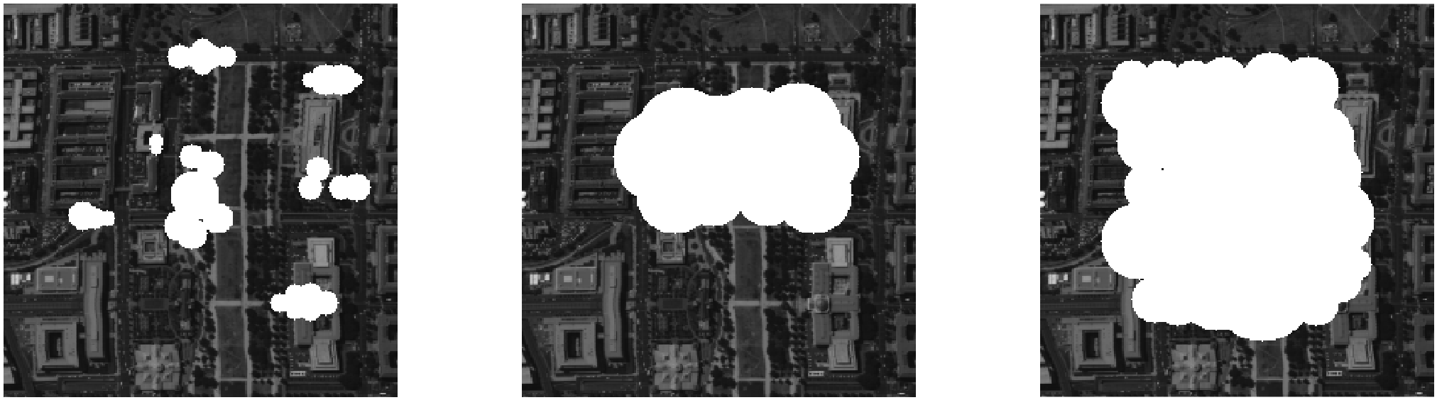
Remote sensing images are easily affected by climate factors, for example, cloud cover is one of the influencing factors. Cloud removal from remote sensing images can improve the effectiveness and availability of remote sensing data, which has very important practical significance. We conduct our experiments on a subimage of the Washington DC Mall data set of size $256\times 256\times 10$ and simulate three cases of cloud cover, as shown in Figure 8. We adopt the parameter settings $\left(\alpha_{1},\alpha_{2},\alpha_{3}\right)=\left(\frac{1}{3},\frac{1}{3},\frac{1}{3}\right)$ , $w=\left(w_{1},w_{2},w_{3}\right)=\left(1,1,1\right)$ , $\mu=0.05$ , $\rho=5\times 10^{-6}$ and the MTT rank is the same as in subsection 5.3. Table 7 displays the experimental results of all methods. We can see that MTTD3R and LRTC-TV-I have comparable performance, but the running time of MTTD3R is half shorter than that of LRTC-TV-I. HaLRTC provides mediocre performance but takes the longest time.

Methods	Case I	Case II	Case III
Methods	MPSNR/MSSIM/time	MPSNR/MSSIM/time	MPSNR/MSSIM/time
MTTD3R	30.37/0.94/44.97	25.44/0.85/47.96	22.77/0.69/59.92
TCTF	21.82/0.92/8.92	15.23/0.80/14.73	12.55/0.59/15.34
LRTC-TV-I	30.33/0.95/105.96	24.02/0.86/123.82	20.42/0.69/145.92
TTD2R	28.51/0.93/61.71	24.78/0.84/58.74	22.45/0.68/64.33
TMac-dec	23.22/0.91/8.75	19.48/0.80/7.37	16.49/0.58/6.97
TMac-inc	23.27/0.91/7.96	19.37/0.80/7.35	16.41/0.58/6.21
HaLRTC	24.97/0.92/302.74	20.12/0.80/281.82	16.93/0.58/309.25

\setcaptionwidth

0.7

Table 7: The PSNR/SSIM/Running time of recovered remote sensing images by different methods on the Washington DC Mall.

6 Conclusion

In this article, we generalize the tensor train factorization to the mode-k tensor train factorization and established a relationship between mode-k TT rank and Tucker rank. We propose a novel multi-mode TT factorization based completion model, and model visual data as the corresponding low-MTT-rank component. Then, we integrated spatial-spectral characteristics into the proposed model and obtain an improved model. We develop an efficient PAM-based algorithm with theoretical and empirical convergence. Comparing MTTD3R with the state-of-the-art completion and approximation methods such as TCTF, LRTC-TV-I, TCTF, TTD2R, TMac-dec, TMac-inc, and HaLRTC, extensive experimental results demonstrate that the proposed MTTD3R method has superiorities of better recovering the missing entries and finely preserving the inherent structure.

References

[1] Xi-Le Zhao, Wen-Hao Xu, Tai-Xiang Jiang, Yao Wang, and Michael K Ng. Deep plug-and-play prior for low-rank tensor completion. Neurocomputing, 400:137–149, 2020.
[2] Yong Chen, Ting-Zhu Huang, Xi-Le Zhao, and Liang-Jian Deng. Hyperspectral image restoration using framelet-regularized low-rank nonnegative matrix factorization. Applied Mathematical Modelling, 63:128–147, 2018.
[3] Yu-Bang Zheng, Ting-Zhu Huang, Xi-Le Zhao, Tai-Xiang Jiang, Tian-Hui Ma, and Teng-Yu Ji. Mixed noise removal in hyperspectral image via low-fibered-rank regularization. IEEE Transactions on Geoscience and Remote Sensing, 58(1):734–749, 2019.
[4] Yangyang Xu, Ruru Hao, Wotao Yin, and Zhixun Su. Parallel matrix factorization for low-rank tensor completion. arXiv preprint arXiv:1312.1254, 2013.
[5] Ji Liu, Przemyslaw Musialski, Peter Wonka, and Jieping Ye. Tensor completion for estimating missing values in visual data. IEEE transactions on pattern analysis and machine intelligence, 35(1):208–220, 2012.
[6] Pan Zhou, Canyi Lu, Zhouchen Lin, and Chao Zhang. Tensor factorization for low-rank tensor completion. IEEE Transactions on Image Processing, 27(3):1152–1163, 2017.
[7] Zemin Zhang, Gregory Ely, Shuchin Aeron, Ning Hao, and Misha Kilmer. Novel methods for multilinear data completion and de-noising based on tensor-svd. In Proceedings of the IEEE conference on computer vision and pattern recognition, pages 3842–3849, 2014.
[8] Xutao Li, Yunming Ye, and Xiaofei Xu. Low-rank tensor completion with total variation for visual data inpainting. In Proceedings of the AAAI Conference on Artificial Intelligence, volume 31, 2017.
[9] Meng Ding, Ting-Zhu Huang, Si Wang, Jin-Jin Mei, and Xi-Le Zhao. Total variation with overlapping group sparsity for deblurring images under cauchy noise. Applied Mathematics and Computation, 341:128–147, 2019.
[10] Emmanuel J Candès and Benjamin Recht. Exact matrix completion via convex optimization. Foundations of Computational mathematics, 9(6):717–772, 2009.
[11] Na Liu, Lu Li, Wei Li, Ran Tao, James E Fowler, and Jocelyn Chanussot. Hyperspectral restoration and fusion with multispectral imagery via low-rank tensor-approximation. IEEE Transactions on Geoscience and Remote Sensing, 2021.
[12] Leonid I Rudin, Stanley Osher, and Emad Fatemi. Nonlinear total variation based noise removal algorithms. Physica D: nonlinear phenomena, 60(1-4):259–268, 1992.
[13] Teng-Yu Ji, Ting-Zhu Huang, Xi-Le Zhao, Tian-Hui Ma, and Gang Liu. Tensor completion using total variation and low-rank matrix factorization. Information Sciences, 326:243–257, 2016.
[14] Misha E Kilmer, Karen Braman, Ning Hao, and Randy C Hoover. Third-order tensors as operators on matrices: A theoretical and computational framework with applications in imaging. SIAM Journal on Matrix Analysis and Applications, 34(1):148–172, 2013.
[15] Misha E Kilmer and Carla D Martin. Factorization strategies for third-order tensors. Linear Algebra and its Applications, 435(3):641–658, 2011.
[16] Ivan V Oseledets. Tensor-train decomposition. SIAM Journal on Scientific Computing, 33(5):2295–2317, 2011.
[17] Oguz Semerci, Ning Hao, Misha E Kilmer, and Eric L Miller. Tensor-based formulation and nuclear norm regularization for multienergy computed tomography. IEEE Transactions on Image Processing, 23(4):1678–1693, 2014.
[18] Johann A Bengua, Ho N Phien, Hoang Duong Tuan, and Minh N Do. Efficient tensor completion for color image and video recovery: Low-rank tensor train. IEEE Transactions on Image Processing, 26(5):2466–2479, 2017.
[19] Hao Zhang, Xi-Le Zhao, Tai-Xiang Jiang, Michael K Ng, and Ting-Zhu Huang. Multiscale feature tensor train rank minimization for multidimensional image recovery. IEEE Transactions on Cybernetics, 2021.
[20] Yao Wang, Jiangjun Peng, Qian Zhao, Yee Leung, Xi-Le Zhao, and Deyu Meng. Hyperspectral image restoration via total variation regularized low-rank tensor decomposition. IEEE Journal of Selected Topics in Applied Earth Observations and Remote Sensing, 11(4):1227–1243, 2017.
[21] Yao Wang, Yishan Han, Kaidong Wang, and Xi-Le Zhao. Total variation regularized nonlocal low-rank tensor train for spectral compressive imaging. Signal Processing, page 108464, 2022.
[22] Hédy Attouch, Jérôme Bolte, Patrick Redont, and Antoine Soubeyran. Proximal alternating minimization and projection methods for nonconvex problems: An approach based on the Kurdyka-Łojasiewicz inequality. Mathematics of operations research, 35(2):438–457, 2010.
[23] Xue-Lei Lin, Michael K Ng, and Xi-Le Zhao. Tensor factorization with total variation and tikhonov regularization for low-rank tensor completion in imaging data. Journal of Mathematical Imaging and Vision, 62(6):900–918, 2020.
[24] Ching-Yun Ko, Kim Batselier, Lucas Daniel, Wenjian Yu, and Ngai Wong. Fast and accurate tensor completion with total variation regularized tensor trains. IEEE Transactions on Image Processing, 29:6918–6931, 2020.
[25] Hédy Attouch, Jérôme Bolte, and Benar Fux Svaiter. Convergence of descent methods for semi-algebraic and tame problems: proximal algorithms, forward–backward splitting, and regularized gauss–seidel methods. Mathematical Programming, 137(1):91–129, 2013.
[26] Dali Chen, YangQuan Chen, and Dingyu Xue. Fractional-order total variation image denoising based on proximity algorithm. Applied Mathematics and Computation, 257:537–545, 2015.
[27] Ryan Wen Liu, Lin Shi, Wenhua Huang, Jing Xu, Simon Chun Ho Yu, and Defeng Wang. Generalized total variation-based mri rician denoising model with spatially adaptive regularization parameters. Magnetic resonance imaging, 32(6):702–720, 2014.
[28] Zhou Wang, Alan C Bovik, Hamid R Sheikh, and Eero P Simoncelli. Image quality assessment: from error visibility to structural similarity. IEEE transactions on image processing, 13(4):600–612, 2004.