Quantum contextuality provides communication complexity advantage
Abstract
Despite the conceptual importance of contextuality in quantum mechanics, there is a hitherto limited number of applications requiring contextuality but not entanglement. Here, we show that for any quantum state and observables of sufficiently small dimensions producing contextuality, there exists a communication task with quantum advantage. Conversely, any quantum advantage in this task admits a proof of contextuality whenever an additional condition holds. We further show that given any set of observables allowing for quantum state-independent contextuality, there exists a class of communication tasks wherein the difference between classical and quantum communication complexities increases as the number of inputs grows. Finally, we show how to convert each of these communication tasks into a semi-device-independent protocol for quantum key distribution.
Introduction.—Contextuality is one of the most significant properties of quantum mechanics Bell 1966; Kochen and Specker 1967; Klyachko et al. 2008; Cabello 2008; Cabello et al. 2014; Budroni et al. 2022. It stipulates that, for some correlations, there is no probability distribution in agreement with the marginal distributions corresponding to sets of compatible (i.e., jointly measurable) observables. In particular, contextuality forbids us to assign predetermined context-independent values to the outcomes of quantum sharp measurements (defined as those that yield the same outcome when they are repeated and do not disturb any compatible observable). While nonlocality which can be seen as a form of quantum contextuality requiring entanglement, has found many applications in quantum communication Ekert 1991; Buhrman et al. 2010; Cubitt et al. 2010, so far, entanglement unassisted quantum contextuality has found few applications despite of its conceptual importance Kleinmann et al. 2011; Howard et al. 2014; Cabello et al. 2018; Grudka et al. 2014; Singh et al. 2017; Saha et al. 2019; Bharti et al. 2019; Saha et al. 2020; Emeriau et al. 2022 11 1 There is other notion of contextuality, preparation contextuality Spekkens 2005, which has found application in oblivious multiplexing and state discrimination tasks Spekkens et al. 2009; Ghorai and Pan 2018; Schmid and Spekkens 2018.
Here, we first show that any contextual correlations achieved using quantum systems of sufficiently small dimensions offer a quantum advantage in a suitably designed one-way communication complexity (or distributed computation) task. Conversely, whenever an additional condition holds, any quantum protocol providing advantage in those tasks produces a proof of contextuality. By itself, this result provides an operational way to understand the sense in which some famous forms of quantum contextuality (notably, the one produced by the violation of the Klyachko-Can-Binicioğlu-Shumovsky inequality with quantum systems of dimension three Klyachko et al. 2008) are “nonclassical”.
As a second result, we show that for every form of state-independent (SI) contextuality Cabello 2008; Badzia¸g et al. 2009; Yu and Oh 2012; Kleinmann et al. 2012, the ratio between the dimensions of the classical systems and quantum systems required to accomplish the task can be made arbitrarily large by increasing the number of inputs. These communication complexity tasks are the so-called equality problems that appear in many practical scenarios Kushilevitz and Nisan 2006; Roughgarden 2016; Rao and Yehudayoff 2020. Finally, we present a semi-device-independent (SDI) protocol for quantum key distribution (QKD) Pawłowski and Brunner 2011 based on the quantum advantage in our communication complexity tasks, in which security is proven by using the monogamy relation Ramanathan et al. 2012; Kurzyński et al. 2014; Saha and Ramanathan 2017 of contextuality.
Contextuality witnesses.—Given a set of events produced in a contextuality experiment, one can define an -vertex graph in which each event is represented by a vertex and exclusive events correspond to adjacent vertices. is called the graph of exclusivity of . In quantum mechanics, each event is represented by a projector . Mutually exclusive events are represented by mutually orthogonal projectors. A quantum realization of a set of events with graph of exclusivity is a set of projectors that satisfies all the exclusivity relations in and all the constraints imposed by the definition of the events.
Definition 1 (Contextuality witness).
A functional
| (1) |
where and is the probability of event , is a quantum contextuality witness if there is a quantum realization of and a quantum state such that
| (2) |
where is the independence number of the vertex-weighted graph , where is the graph of exclusivity of and . That is, is the largest value of , where is the set of the subsets consisting of nonadjacent vertices of Bondy and Murty 1976.
The name ‘contextuality witness’ follows from the fact that, given , one can find a noncontextuality inequality Cabello 2016; Cabello 2021 whose upper bound for noncontextual models is and whose quantum value is the left-hand side of Eq. (2) Cabello 2016; Cabello 2021; Cabello et al. 2014.
We will focus on quantum realizations of contextuality witnesses constructed as follows. We first identify a vertex-weighted graph for which we can identify and such that Eq. (2) holds. We will refer to as a quantum realization of a contextuality witness for . In some cases, there is no need to identify a state .
Definition 2 (State-independent contextuality witness).
If we have satisfying Eq. (2) that includes projectors that are not of rank one, we can obtain satisfying Eq. (2) by splitting each of the projectors that are not rank one into rank-one projectors. See Appendix A.
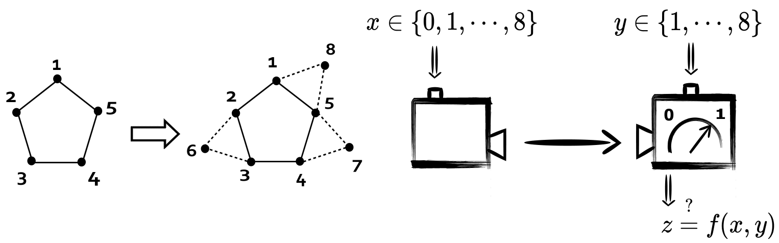
One-way communication complexity.—Communication complexity Kushilevitz and Nisan 2006 studies the amount of communication required for tasks involving inputs distributed among several parties. In one-way communication complexity Kushilevitz and Nisan 2006; de Wolf 2002; Buhrman et al. 2010; Buhrman et al. 1998, there are two parties. As shown in Fig. 1, in each round, Alice, receives a random input . Depending upon , Alice sends a message (classical or quantum) to Bob. In addition, Bob receives a random input . Using and the message received from Alice, Bob outputs which is Bob’s guess about a certain function . After many rounds, they produce the probability of , given inputs and . The figure of merit of the task is given by
| (3) |
where and . We are interested in two aspects. Firstly, the maximum value of that can be achieved under the restriction that the dimension of the (classical or quantum) system communicated from Alice to Bob is . Secondly, the minimum dimensional (classical or quantum) system required to communicate in order to achieve a certain value of . Sharing prior classical randomness between Alice and Bob is allowed.
Communication complexity advantage based on quantum contextuality witnesses.— Consider satisfying Eq. (2) and such that . Since , without loss of generality, we can take . The task is defined as follows. First, we consider an extended graph by adding additional vertices to such that each vertex in belongs to, at least, one clique of size . A clique is a set of vertices in which every pair are adjacent. We thereupon assign additional vectors (or rank-one projectors) to those additional vertices, so each vector belongs to at least one basis within the new set of vectors; see Fig. 1. Alice receives and Bob receives , where number of vertices is added. Bob outputs his guess for
| (4) |
where is the set of the vertices that are adjacent to (i.e., neighbors of) in . In other words, Bob needs to distinguish the runs where and from the runs where . Except for these, whenever and , or, and , the runs do not contribute to the figure of merit of the communication task. That is, the task for Alice and Bob is to maximize
| (5) |
where
| (6) |
thus . Alice and Bob must accomplish this task with the restriction that the dimension of the (classical or quantum) system communicated between them is . Therefore, the communication task is fully specified by the value of , the extended graph , and the weights . The important point is that there is quantum advantage in this communication task whenever is “sufficiently small” in the sense that , where is the chromatic number of the graph 22 2 Chromatic number is the smallest number of colors needed to color the vertices of so that no two adjacent vertices share the same color Bondy and Murty 1976.
Result 1.
In a general quantum strategy, let denote the quantum state sent by Alice to Bob upon receiving , and let denote the quantum measurement Bob performs on to obtain , upon receiving input . Suppose that is a contextuality witness satisfying Eq. (2). Since, the projectors in are of rank one, one can always add rank-one projectors so that the extended set has the relations of orthogonality given by . Given , Alice and Bob choose an extended set and apply the following strategy:
| (7) |
This way, , so the value of in Eq. (5) is
| (8) |
while communicating a (quantum) system of dimension between Alice and Bob. In contrast to that,
Theorem 1.
Whenever , for any strategy in which the system communicated between Alice and Bob is a classical system of dimension , the value of is upper bounded by
| (9) |
where is the minimum number of “improperly colored” vertices of when colors are used to color all the vertices. A vertex is improperly colored if it has at least one neighbor sharing the same color.
For a proof, see Appendix B. Because of Eq. (2) and the fact that is non-negative, the expression in Eq. (8) is strictly larger than .
Let us suppose that is the minimum dimension in which the set of projectors and can be realized such that is a contextuality witness. For any SI contextuality witness, Cabello 2011; Ramanathan and Horodecki 2014; Cabello et al. 2015. Therefore, whenever , there will be at least two adjacent vertices sharing the same color when colors are used to color the graph, implying . Moreover, in this case, can be any quantum state in .
Explicit examples of the quantum advantage for communication complexity tasks based on some quantum SI contextuality sets are presented in Appendix D, together with a proof of their robustness against white noise.
Certifying contextuality witness from communication complexity task.—The quantum communication strategy given by Eq. (Quantum contextuality provides communication complexity advantage) is based on a contextuality witness. However, a general quantum strategy with advantage consists of a set of states acting on and a set of measurement so that the value of is greater than . In general, such a strategy may not be related to contextuality witnesses. Nevertheless, the following theorem allows us to identify whether or not an unknown quantum communication strategy admits a contextuality witness.
Theorem 2.
For the above introduced communication task defined by , the following condition holds:
| (10) |
if and only if is a set of rank-one projectors that has as graph of orthogonality and .
For a proof, see Appendix B. Therefore, Theorem 2 presents operational criteria to certify a set of rank-one projectors satisfying orthogonality relations according to a graph. Note that the probabilities in Eq. (10) are the first two terms of . Consider the particular case of the task (5) in which and an unknown quantum strategy comprising , that provides greater value than . First, it follows from Eq. (9) that, in this case, since . In addition to that, if the first two terms in attain their algebraic values, then Theorem 2 implies must be a contextuality witness.
Increasing advantage in communication complexity.—Here, we will consider only those contextuality witnesses where . In these cases, it suffices to consider a simplified version of the above-described communication complexity task by taking the first two terms of . Therefore, the figure of merit will be
| (11) |
where . Here, the communication problem is solely based on the exclusivity graph Saha et al. 2019, and we do not need to consider additional inputs apart from the set of vertices of . More importantly, this is an equality problem as Bob guesses whether his input is equal to or not Kushilevitz and Nisan 2006.
Let (or ) be the minimum dimension of quantum system (or classical system) that should be communicated to achieve . We are now interested in quantum advantages in terms of and . A quantum advantage in communication complexity implies , or, equivalently, conventionally expressed in terms of classical and quantum bits.
Theorem 3.
Given any witness where ,
| (12) |
Moreover, is the minimum dimension such that there exists a set of projectors acting on satisfying the orthogonality relations given by .
A proof is provided in Appendix B. We can readily check that the quantum strategy, , yields . Thus, we have an advantage whenever . In order to observe an increasing advantage, we need to consider products of graphs.
Definition 3 (Inclusive graph product or co-normal product or disjunctive product or OR product ).
The vertex set of the inclusive graph product of two graphs is . The edges of are defined as iff or . We denote by the -times product of the same graph Feige 1997; Feige 1995.
Theorem 4.
Given a graph with vertices, the ratio between classical and quantum communication complexities of based on , that is, increases polynomially with ,
| (13) |
where is the fractional chromatic number of Ramanathan and Horodecki 2014. For any graph, .
For a proof, see Appendix B. Since for any quantum SI contextuality set in dimension Ramanathan and Horodecki 2014; Cabello et al. 2015, the right-hand-side of (13) can be arbitrarily large as increases 33 3 Note that is lower bounded by the size of the maximum clique, i.e., the clique of largest size, of .. It follows from (13) that the difference between the classical and quantum complexities for the equality task based on is lower bounded by bits, which increases with . In Table 1, we present some explicit examples of the quantum advantage.
| SI witness | from Eq. (13) | ||
|---|---|---|---|
| with | so that qubits | ||
| YO-13 Yu and Oh 2012 | 3 | 35/11 | |
| Peres-33 Peres 1991 | 3 | 13/4 | |
| CEG-18 Cabello et al. 1996 | 4 | 9/2 | |
| Pauli-240 Xu et al. 2023 | 8 | 15 | |
| Pauli-4320 Xu et al. 2023 | 16 | 60 |
Before proceeding to the next section, we point out an example of SI witness and the respective equality problem where the separation between the classical and quantum communication complexities grows exponentially with the dimension. Consider the set of vectors in of the form where such that in every vector the number of taking value is even. Note that there are such vectors in , and let us denote this set by . The graph, say , representing the orthogonality relations for this set of vectors was introduced by Newman Newman 2004 and has been recently studied in the context of application of contextuality Xu et al. 2023. It turns out for any and divisible by 4, is SI contextuality witness where for all (see Appendix C for the proof). Remarkably, for the equality problem defined by (11) with respect to , we have
| (14) |
Thus, the gap between classical and quantum complexities is at least bits. The detailed proof of this fact is provided in Appendix C, which follows from the results by Frankl-Rödl Frankl and Rodl 1987.
Semi-device-independent quantum key distribution.—Here, we propose that a QKD protocol based on quantum advantage in the communication complexity task introduced by in Eq. (5) where is taken to be . Unlike fully device-dependent protocols Bennett and Brassard 2014; Singh et al. 2017, our protocol is semi-device-independent Pawłowski and Brunner 2011 involving two black boxes - Alice’s preparation device and Bob’s measurement device. We only assume that () the dimension of the degrees-of-freedom (of the physical system), in which the information is encoded, is bounded by , and () the devices may share classical randomness but that is uncorrelated with the choices of the inputs .
The QKD protocol is as follows. After completing a large number of runs, Alice randomly chooses some runs and publicly announces her input so that Bob can verify that the obtained value of the figure of merit is greater than . Thereby, Bob is ensured that the probabilities produced by his device cannot be simulated by classical systems under the aforementioned assumptions. Bob publicly announces his input for the remaining runs. Subsequently, Alice notes down according to Eq. (4) as the shared key. Whenever , or, and , Alice publicly announces that the transmission is unsuccessful.
It is not difficult to show that such QKD protocol is secure against restricted eavesdroppers whenever the contextuality witness satisfies monogamy relations that are proposed in Ramanathan et al. 2012. The monogamy relation between two witnesses of contextuality realized on two separate degrees-of-freedom of any quantum state implies
| (15) |
for any , where , realize the respective exclusivity graph . Such relation holds for a large class of contextuality witnesses, including the well-known odd-cycle witnesses Ramanathan et al. 2012. The QKD protocol is secure if the mutual information of Alice-Bob is greater than the mutual information of Alice-Eve Pawłowski and Brunner 2011, i.e., , which for individual attacks and binary output implies , taking be the value of obtained by Bob (Eve). Since Eve also knows the input , she and Bob are in the same state to guess . Because of Theorem 2, when Bob observes that the first two terms in attain their maximal values, then are rank-one projectors realizing . We assume that for Eve also realizes . Now, even if Eve shares arbitrary quantum correlation with the preparation device of Alice, due to monogamy relation (15), the following holds true:
| (16) |
Taking the best possible scenario for Eve in which she also observes (10), the above relation implies
| (17) |
Therefore, whenever Alice-Bob obtains quantum advantage, that is, , the protocol is secure against such eavesdropping. Subsequently, the key rate can be obtained by (see Table (2) in Appendix D).
In addition to the QKD protocol, these communication tasks can also be used to generate quantum randomness in the prepare-and-measure scenario Li et al. 2012; Lunghi et al. 2015; Han et al. 2016. We have discussed this in Appendix E.
Conclusions.—This work shows that all forms of quantum contextuality with sufficiently small dimension provide quantum advantage in distributed computation and in various communication protocols without requiring entanglement. In distributed computation, equality problems are essential for implementing large-scale circuits and data verification Kushilevitz and Nisan 2006; Roughgarden 2016; Rao and Yehudayoff 2020 (see Appendix F). We show the existence of a variant of the equality problem pertaining to every vertex-weighted graph with certain properties providing an advantage over classical communication.
Considering equality problems defined by the graphs of a large class of contextuality witnesses including all quantum state-independent contextuality witnesses, we show that the communication complexity required to execute such problems in classical theory is larger than that in quantum theory. Moreover, the complexity advantage increases with an increase in the number of inputs, identifying a class of equality problems that can be solved only in quantum communication.
As further applications of quantum contextuality driven communication tasks, we show how such
tasks can be used for semi-device-independent QKD, as
well as for the purpose of randomness generation. As interesting open problems for further work, we point out the possibility of extending the security proof of the QKD protocol to arbitrary individual eavesdropping strategies and finding optimal communication complexity advantages.
It would also be interesting to extend the link between quantum contextuality and quantum advantage in communication complexity tasks involving more than two parties, like, quantum fingerprinting Buhrman et al. 2001.
Acknowledgements.— D. S. acknowledges National Post-Doctoral Fellowship (PDF/2020/001682) for support. A. C. is supported by Project Qdisc (Project No. US-15097, Universidad de Sevilla), with FEDER funds, QuantERA grant SECRET, by MINECO (Project No. PCI2019-111885-2), and MICINN (Project No. PID2020-113738GB-I00). A. S. M. acknowledges support from Project No. DST/ICPS/QuEST/2018/98 of the Department of Science & Technology, Government of India.
References
- Bell (1966) J. S. Bell, Rev. Mod. Phys. 38, 447 (1966).
- Kochen and Specker (1967) S. Kochen and E. P. Specker, J. Math. Mech. 17, 59 (1967).
- Klyachko et al. (2008) A. A. Klyachko, M. A. Can, S. Binicioğlu, and A. S. Shumovsky, Phys. Rev. Lett. 101, 020403 (2008).
- Cabello (2008) A. Cabello, Phys. Rev. Lett. 101, 210401 (2008).
- Cabello et al. (2014) A. Cabello, S. Severini, and A. Winter, Phys. Rev. Lett. 112, 040401 (2014).
- Budroni et al. (2022) C. Budroni, A. Cabello, M. Kleinmann, J.-Å. Larsson, and O. Gühne, Rev. Mod. Phys. (2022).
- Ekert (1991) A. K. Ekert, Phys. Rev. Lett. 67, 661 (1991).
- Buhrman et al. (2010) H. Buhrman, R. Cleve, S. Massar, and R. de Wolf, Rev. Mod. Phys. 82, 665 (2010).
- Cubitt et al. (2010) T. S. Cubitt, D. Leung, W. Matthews, and A. Winter, Phys. Rev. Lett. 104, 230503 (2010).
- Kleinmann et al. (2011) M. Kleinmann, O. Gühne, J. R. Portillo, J.-Å. Larsson, and A. Cabello, New J. Phys. 13, 113011 (2011).
- Howard et al. (2014) M. Howard, J. Wallman, V. Veitch, and J. Emerson, Nature 510, 351 (2014).
- Cabello et al. (2018) A. Cabello, M. Gu, O. Gühne, and Z.-P. Xu, Phys. Rev. Lett. 120, 130401 (2018).
- Grudka et al. (2014) A. Grudka, K. Horodecki, M. Horodecki, P. Horodecki, R. Horodecki, P. Joshi, W. Kłobus, and A. Wójcik, Phys. Rev. Lett. 112, 120401 (2014).
- Singh et al. (2017) J. Singh, K. Bharti, and Arvind, Phys. Rev. A 95, 062333 (2017).
- Saha et al. (2019) D. Saha, P. Horodecki, and M. Pawłowski, New J. Phys. 21, 093057 (2019).
- Bharti et al. (2019) K. Bharti, M. Ray, A. Varvitsiotis, N. Warsi, A. Cabello, and L. Kwek, Phys. Rev. Lett. 122, 250403 (2019).
- Saha et al. (2020) D. Saha, R. Santos, and R. Augusiak, Quantum 4, 302 (2020).
- Emeriau et al. (2022) P.-E. Emeriau, M. Howard, and S. Mansfield, PRX Quantum 3, 020307 (2022).
- (19) There is other notion of contextuality, preparation contextuality Spekkens 2005, which has found application in oblivious multiplexing and state discrimination tasks Spekkens et al. 2009; Ghorai and Pan 2018; Schmid and Spekkens 2018.
- Badzia¸g et al. (2009) P. Badzia¸g, I. Bengtsson, A. Cabello, and I. Pitowsky, Phys. Rev. Lett. 103, 050401 (2009).
- Yu and Oh (2012) S. Yu and C. H. Oh, Phys. Rev. Lett. 108, 030402 (2012).
- Kleinmann et al. (2012) M. Kleinmann, C. Budroni, J.-Å. Larsson, O. Gühne, and A. Cabello, Phys. Rev. Lett. 109, 250402 (2012).
- Kushilevitz and Nisan (2006) E. Kushilevitz and N. Nisan, Communication Complexity (Cambridge Univ Press, Cambridge, UK, 2006).
- Roughgarden (2016) T. Roughgarden, Communication Complexity (for Algorithm Designers), Foundations and Trends® in Theoretical Computer Science 11, 217 (2016).
- Rao and Yehudayoff (2020) A. Rao and A. Yehudayoff, Communication Complexity: and Applications (Cambridge University Press, 2020).
- Pawłowski and Brunner (2011) M. Pawłowski and N. Brunner, Phys. Rev. A 84, 010302 (2011).
- Ramanathan et al. (2012) R. Ramanathan, A. Soeda, P. Kurzyński, and D. Kaszlikowski, Phys. Rev. Lett. 109, 050404 (2012).
- Kurzyński et al. (2014) P. Kurzyński, A. Cabello, and D. Kaszlikowski, Phys. Rev. Lett. 112, 100401 (2014).
- Saha and Ramanathan (2017) D. Saha and R. Ramanathan, Phys. Rev. A 95, 030104 (2017).
- Bondy and Murty (1976) J. A. Bondy and U. S. R. Murty, Graph Theory with Applications (Macmillan, London, 1976).
- Cabello (2016) A. Cabello, Phys. Rev. A 93, 032102 (2016).
- Cabello (2021) A. Cabello, Phys. Rev. Lett. 127, 070401 (2021).
- de Wolf (2002) R. de Wolf, Theor. Comput. Sci. 287, 337 (2002).
- Buhrman et al. (1998) H. Buhrman, R. Cleve, and A. Wigderson, in Proceedings of the Thirtieth Annual ACM Symposium on Theory of Computing (1998) p. 63.
- (35) Chromatic number is the smallest number of colors needed to color the vertices of so that no two adjacent vertices share the same color Bondy and Murty 1976.
- Cabello (2011) A. Cabello, “State-independent quantum contextuality and maximum nonlocality,” (2011), arXiv:1112.5149 .
- Ramanathan and Horodecki (2014) R. Ramanathan and P. Horodecki, Phys. Rev. Lett. 112, 040404 (2014).
- Cabello et al. (2015) A. Cabello, M. Kleinmann, and C. Budroni, Phys. Rev. Lett. 114, 250402 (2015).
- Feige (1997) U. Feige, Combinatorica 17, 79 (1997).
- Feige (1995) U. Feige, in Proceedings of the Twenty-Seventh Annual ACM Symposium on Theory of Computing (ACM, New York, 1995) p. 635.
- (41) Note that is lower bounded by the size of the maximum clique, i.e., the clique of largest size, of .
- Peres (1991) A. Peres, J. Phys. A: Math. Gen. 24, L175 (1991).
- Cabello et al. (1996) A. Cabello, J. Estebaranz, and G. García-Alcaine, Phys. Lett. A 212, 183 (1996).
- Xu et al. (2023) Z.-P. Xu, J. Steinberg, J. Singh, A. J. López-Tarrida, J. R. Portillo, and A. Cabello, Quantum 7, 922 (2023).
- Newman (2004) M. W. Newman, Independent sets and eigenspaces (University of Waterloo, 2004).
- Frankl and Rodl (1987) P. Frankl and V. Rodl, Trans. Am. Math. Soc. 300, 259 (1987).
- Bennett and Brassard (2014) C. H. Bennett and G. Brassard, Theor. Comput. Sci. 560, 7 (2014).
- Li et al. (2012) H.-W. Li, M. Pawłowski, Z.-Q. Yin, G.-C. Guo, and Z.-F. Han, Phys. Rev. A 85, 052308 (2012).
- Lunghi et al. (2015) T. Lunghi, J. B. Brask, C. C. W. Lim, Q. Lavigne, J. Bowles, A. Martin, H. Zbinden, and N. Brunner, Phys. Rev. Lett. 114, 150501 (2015).
- Han et al. (2016) Y.-G. Han, Z.-Q. Yin, H.-W. Li, W. Chen, S. Wang, G.-C. Guo, and Z.-F. Han, Phys. Rev. A 93, 032332 (2016).
- Buhrman et al. (2001) H. Buhrman, R. Cleve, J. Watrous, and R. de Wolf, Phys. Rev. Lett. 87, 167902 (2001).
- Spekkens (2005) R. W. Spekkens, Phys. Rev. A 71, 052108 (2005).
- Spekkens et al. (2009) R. W. Spekkens, D. H. Buzacott, A. J. Keehn, B. Toner, and G. J. Pryde, Phys. Rev. Lett. 102, 010401 (2009).
- Ghorai and Pan (2018) S. Ghorai and A. K. Pan, Phys. Rev. A 98, 032110 (2018).
- Schmid and Spekkens (2018) D. Schmid and R. W. Spekkens, Phys. Rev. X 8, 011015 (2018).
Appendix A Contextuality witness of rank-one projectors
Lemma 1.
For any satisfying Eq. (2) in the main text, where the rank of is , there is satisfying (2) such that
| (18) |
where and, for each , and is a vertex-weighted subgraph of .
Proof.
If the rank of is , then we split the vertex into vertices, say , where . The edges and weights of the new graph are defined as follows:
| (19) |
Eq. (19) implies that . Now, if we split each projector according to (18), then the set of rank-one projectors has as the graph of orthogonality. Furthermore,
| (20) |
which is greater than by definition.
Appendix B Communication complexity advantage based on quantum contextuality
We first state a general feature of communication tasks in the following lemma, which will be used later in the proof of the theorems.
Lemma 2.
The maximum value of in Eq. (3), when the system communicated between Alice and Bob is a classical system of dimension , is given by
| (21) |
where , and, , .
Proof.
Alice and Bob share prior classical random variables with arbitrary distribution . Alice’s strategy is to encode the information of input into classical message . A general description of such a strategy is given by a set of probabilities , where is the probability of sending the message depending on input choice and random variable . Here , since the dimension of the communicated system is at most . Bob’s decoding strategy is generally represented by the set of probability distribution , where is the probability of output given his input , received message , and the shared random variable . Therefore, the general expression of the probability of getting outcome upon receiving inputs in classical communication is given by
| (22) |
By dividing all inputs into two subgroups according to the value of given every and substituting each term using the above in the figure of merit, we find that
| (23) |
Let us see the term within the curly bracket . Since the best decoding probability is fixed such that the above expression is
| (24) |
Given any encoding probability , the above expression within the square bracket is a convex function of , and thus, without loss of generality, we can take for which that expression is maximum or, equivalently, we can omit the dependence of . This implies
| (25) |
Further, using the identity, for any non-negative number , Eq. (25) further reduces to
| (26) |
Using , and in the above equation, we get (21). Finally, note that it is sufficient to consider the extremal values of since the expression is convex.
Proof of Theorem 1.
Using Eq. (21) for given by Eq. (5), we can express the optimal classical value as follows:
| (27) | |||||
wherein the encoding strategy is deterministic, that is, for each input , Alice sends a classical level out of distinct levels. This is equivalent to assigning one of the colors to each input . Since , in general, colors are not sufficient to color all the vertices of the extended properly. Say is the minimum number of ‘improperly colored’ vertices when colors are used to color all the vertices of the extended exclusivity graph. A vertex is ‘improperly colored’ if it has at least one neighbour that shares the same color. We would like to find the optimal encoding strategy that maximizes in (27). Say, the optimal encoding is such that, there are improperly colored vertices, that is, out of all the vertices, vertices are properly colored, where is an integer. Let us denote the level/color by that is assigned to input . There are three possibilities for each input :
- 1.
y is not properly colored. In this case there exists at least one such that . Therefore,
(28) - 2.
y is properly coloured and . In this scenario, either , or, . For the former case, since every belongs to at least one -clique there exists one , for which . Therefore,
(29) Here, we have used our convention for the contextuality witness that,
(30) While for the latter case,
(31) - 3.
y is properly coloured and . In this case,
(32)
As the encoding strategy properly colors vertices, the above analysis implies
| (33) |
Using this in Eq. (27), we obtain
| (34) |
Replacing by from Eq. (6) in the above equation, we obtain
| (35) | |||||
If , then
| (36) |
On the other hand, if , then
| (37) |
where the sum over on right-hand-side is taken for number of different indices. It follows from Eq. (30) that the above is bounded by Therefore, the best strategy is choosing , which implies Eq. (9).
Proof of Theorem 2.
Eq. (10) implies
| (38) |
where denotes the reduced form of in the support of . Note that are projectors and we must have
| (39) |
The size of the maximum clique in the extended graph is . Say, is a maximum clique. The conditions (39) for any pair of and hold true if and only if are rank-one projectors and satisfy orthogonality relations according to . Moreover, it follows from (38) that
| (40) |
However, the normalization condition holds if and only if for all . Due to the fact that every input belongs to at least one maximum clique, the analysis holds true for all .
Proof of Theorem 3.
given by Eq. (11) is if
| (41) |
which implies Eq. (38)-(39). Consequently, satisfies the orthogonality relations as per the exclusivity graph . Moreover, the new set of measurements defined by also achieves for the same Alice’s encoding strategy . Therefore, for any quantum strategy that yields , there exists a set of projectors that realizes . In the reverse direction, for any set of projectors realizing , the strategy in which achieves . So, there is a one-to-one correspondence between quantum strategy achieving the perfect figure of merit and a set of projectors satisfying the orthogonality relations according to . Thus, is the minimum dimension such that a set of projectors acting on exists, and moreover, .
In classical communication, it follows from (21) that
| (42) |
which is 1 if and only if
| (43) |
Since, without loss of generality, we can take to be deterministic, the above implies if for some then . Therefore, the set of can be used to color the graph, and similarly, any set of colors used to color the graph can also be used as to achieve . Thus, is the minimum of number colors required to color the vertices of .
Proof of Theorem 4.
To prove , it suffices to show that there exists a set of projectors realizing in dimensional Hilbert space. Consider the realization where the vertex (where each ) of is represented by the projector . Clearly, if for any , then the respective two projectors are orthogonal as and are orthogonal.
On the other hand, due to Theorem 3, we know that . For any graph , we have . In addition, according to Lemma 2.8 in Ref. Feige 1995. Therefore, Eq. (13)
holds true.
Remark. We have another lower bound on as follows.
| (44) |
Proof.
we make use of Theorem 2.3 of Feige 1997 that states the following relation:
| (45) |
when both graphs and have same number of vertices . Taking to be , we have . Again, we taking product of two of the same number of vertices , we have , and similarly, we can obtain
| (46) |
for any . Finally, using the facts that and the above relation, we arrive at (44).
Appendix C SI contextuality witness and exponential separation in communication complexities
Firstly, we point out the correspondence between the large classical vs. quantum communication complexities gap in distributed Deutsch-Jozsa task Buhrman et al. 1998; Buhrman et al. 2010 and the equality problem (Eq. (11)) with respect to exclusivity graphs. Consider the set of vectors in of the form
| (47) |
where every . There is number of distinct vectors in this set, and two vectors from this set are orthogonal whenever values of ’s are different in exactly number of places. We can consider the graph, often called Hadamard graph , representing the orthogonality relations of the set of vectors in , and thereupon, the equality problem defined by Eq. (11) with respect to .
The result by Frankl-Rödl Frankl and Rodl 1987 implies that , whenever is divisible by (Theorem 1.11 in Frankl and Rodl 1987). Plugging this bound into the general relation , we find that for the Hadamard graph . Therefore, the difference between classical and quantum communication complexities is at least
bits.
We now consider the Newman graph Newman 2004 introduced in the main text. It is defined by the orthogonality relation of the set of vectors in that takes the form (47) where and in every vector the number of taking value is even. There are such vectors in , and we denote this set by . Let us again take to be divisible by 4. It has been pointed out in Xu et al. 2023 that
| (48) |
On the other hand, due to Lemma 6.6.1 of Newman 2004 we know
| (49) |
Consequently, using the aforementioned result by Frankl-Rödl Frankl and Rodl 1987 we have
| (50) |
Comparing the above quantity with the right-hand-side of (48), we see that is SI contextuality witness (where for all ) if
| (51) |
It has been shown in Xu et al. 2023 that is SI contextuality witness for .
In order to get a lower bound on the classical communication complexity of the respective equality problem, we plug the relation (50) into and find that . Finally, since by its construction, we obtain Eq. (14) in the main text.
Appendix D Examples
It follows from Eq. (8) in the main text that the maximum quantum value for from all , with , is given by
| (52) |
where
| (53) |
and is a realization of .
D.1 Robustness of the quantum advantage in communication tasks
Here, we discuss the robustness of the quantum advantage in the presence of white noise. We take to be the sharpness parameter or to be the parameter quantifying the amount of white noise. In such case, the communicated quantum state will be
| (54) |
where is the state that Alice wants to send given in Eq. (7) in the main text. Taking into consideration Bob’s measurements given by Eq. (7) in the main text, the new probabilities are
| (55) |
Substituting these probabilities, we calculate the modified value of as equal to
| (56) |
Now, we reckon the best quantum strategy defined in Eqs. (52)–(53) to find the maximum modified quantum value in the presence of noise is
| (57) |
Using the expression of from Eq. (6) in the main text, we get a simplified form of the above expression,
| (58) |
Subsequently, the quantum advantage persists this modified quantum value is greater than the best classical value, that is,
| (59) |
which, after a reshuffling of parameters, implies
| (60) |
Here, is the critical value of (sharpness parameter) up to which there will not be any quantum advantage. In other words, to observe quantum advantage the sharpness parameter must be greater than . The critical values of the sharpness parameter in our communication task for several well-known contextuality witnesses are computed in the third column of Table 2.
D.2 Communication complexity advantage based on extended 5-cycle graph
Consider the first figure of the 5-cycle graph in Table 2. There are total of five events and three extensions. So, and . We take weighs . The classical bound for this contextuality witness whereas quantum bound . Alice chooses an input from the set . Bob chooses an input from . The task is to maximize the figure of merit in Eq. (5) of the main text. For this, let us first determine using Eq. (6) in the main text. That is,
| (61) |
Using this and in Eq. (9) in the main text, we get the maximum value of the figure of merit with classical settings as . On the other hand, the maximum figure of merit with quantum settings using Eq. (52) is . This shows a quantum advantage. Similarly, we have shown the quantum advantage in the considered communication task for other contextuality witnesses in the third column of Table 2.
D.3 Communication complexity advantages and key rates of the respective QKD protocol based on a few well-known quantum contextuality witnesses
In order to calculate the average key rate per transmission, we compute the Shannon information of the transmitted string which is given as , where is the probability of bit 0(1) in the key. Let be the success probability of generating the key, then the average key generation per transmission or the key rate is . The key rates for some contextuality witnesses are given in Table 2. However, this key rate may not be secure.
The secure key rate () is calculated using Eq. (17). For this, we estimate the mutual information between Alice and Bob/Eve as follows Pawłowski and Brunner 2011:
| (62) |
Here, is the figure of merit of guessing for Bob (Eve), is the Shannon binary entropy. We have taken and . The secure key rates for some contextuality witnesses are also provided in Table 2. Note that Alice and Bob can apply the privacy amplification using Toeplitz matrix-based hash function on raw keys to make it secure.
| NC | Graph | Communication complexity advantage | Quantum key distribution | ||||||||||||||
|---|---|---|---|---|---|---|---|---|---|---|---|---|---|---|---|---|---|
| 5-cycle |
|
|
| ||||||||||||||
| 5-cycle* |
|
|
| ||||||||||||||
| 7-cycle |
|
|
| ||||||||||||||
| CEG-18 |
|
|
| ||||||||||||||
| YO-13 |
|
|
|
Appendix E Randomness certification
Schemes for quantum randomness generation have been proposed based on quantum advantages in communication tasks Li et al. 2012; Lunghi et al. 2015; Han et al. 2016. We can also use the communication complexity task introduced in Eq. (4)-(5) to generate secure random bits from the untrusted preparation and measurement devices under the assumptions ()-() mentioned in the preceding section. The random bits is obtained from the measurement outcome . Notice that for , all the probabilities appearing in the figure of merit (5) are deterministic in the quantum strategies coming from contextuality witnesses. This enforces us to obtain the randomness only when , which is suitably quantified by the minimum entropy function as follows:
| (63) | |||||
| Subject to: |
where is the obtained value of . The above quantity is not necessarily nonzero for any contextuality witness, however, it is nonzero for odd-cycle contextuality witnesses Bharti et al. 2019; Saha et al. 2020. In Figure II, we evaluate for the 5-cycle graph, which is non zero for all and attains the maximum value of .
Appendix F Practical applications of equality problems considered here
The equality problems, given by Eq. (11), have direct practical applications in distributed computation. Same data stored in two stations get altered due to various reasons. Therefore, in distributed computation, it is often required to verify whether the data set in two sites is the same or not. We can consider and to be the data set variables in two stations, such that the variables can change to some specific variables due to the error. Now we can express this problem as an equality problem by a graph wherein the variables representing two adjacent vertices can interchange with each other. Communication complexity provides the minimum communication cost to verify whether the two variables are identical Kushilevitz and Nisan 2006; Rao and Yehudayoff 2020.
Apart from this, communication complexity of equality problems provides upper bounds on query complexity, the complexity of checking two variables are the same or not in a single device Kushilevitz and Nisan 2006. Streaming algorithms, in which all the inputs cannot be processed due to memory constraints, are also modeled as one-way communication complexity problems Roughgarden 2016. Furthermore, communication complexity of any equality problem has a natural application in game theory involving two agents Roughgarden 2016.