Estimation and Inference by Stochastic Optimization
Abstract
In non-linear estimations, it is common to assess sampling uncertainty by bootstrap inference. For complex models, this can be computationally intensive. This paper combines optimization with resampling: turning stochastic optimization into a fast resampling device. Two methods are introduced: a resampled Newton-Raphson (rnr) and a resampled quasi-Newton (rqn) algorithm. Both produce draws that can be used to compute consistent estimates, confidence intervals, and standard errors in a single run. The draws are generated by a gradient and Hessian (or an approximation) computed from batches of data that are resampled at each iteration. The proposed methods transition quickly from optimization to resampling when the objective is smooth and strictly convex. Simulated and empirical applications illustrate the properties of the methods on large scale and computationally intensive problems. Comparisons with frequentist and Bayesian methods highlight the features of the algorithms.
JEL Classification: C2, C3
Keywords: Stochastic gradient descent, M-estimation, out of and multiplier Bootstrap.
1 Introduction
Many empirical economic analyses involve the process of estimating parameters from a sample of observations and assessing sampling uncertainty. The typical routine is to first produce a consistent M-estimator of the true by minimizing the sample objective . Then, standard errors and confidence intervals are computed to perform inferences. Because the sandwich estimator is harder to implement for more complicated models, it is very common to use a bootstrap at that stage. For more computationally intensive nonlinear estimations, it is common to report standard errors based on few bootstrap draws, e.g. 20, 25, or 50.11 1 71 of all papers published in the American Economic Review between 2012 and 2016 relied on bootstrap inference, 49 of them report bootstrap standard errors. More than one in five of those 49 papers use bootstrap replications or fewer to compute standard errors. Survey conducted by the author, details available upon request. The main bottleneck is that each replication requires another estimation on resampled data, which is nontrivial for these complex models. There is a long-standing interest in finding shortcuts to relieve this computational burden without sacrificing too much accuracy. Examples include Davidson and MacKinnon 1999, Andrews 2002, Kline and Santos 2012, and more recently Honoré and Hu 2017. These methods compute standard errors taking a converged estimate as given. As such, estimation always precedes inference.
This paper proposes to combine resampling with optimization to produce estimates, confidence intervals, and standard errors in a single step. This is very close in spirit to Markov-chain Monte Carlo (MCMC) methods that produce draws from a Bayesian posterior to be used for both estimation and inference. Unlike MCMC, the information matrix equality is not required for valid inference. The main loop of the Algorithm is a stochastic optimization routine which evaluates the objective on batches of resampled data with size . Starting from an initial guess , one updates to , , using the resampled gradient and inverse Hessian (or an approximation) as a conditioning matrix, with a fixed learning rate . The Algorithm can also be used with reweighted samples of data. For a suitable choice of and a strictly convex objective , it is shown that the average over draws is equal to up to order . Even with and , the estimates are consistent and asymptotically normal as long as and . The results also show that the distribution, conditional on the sample, of is first-order equivalent to that of , up to scale, and standard errors are consistent. Inference results are valid for a resampled Newton-Raphson (rnr) and a resampled quasi-Newton (rqn) algorithm based on a new quasi-Newton update. For other conditioning matrices, the draws can produce consistent estimates but they need not be valid for inference.
The main theoretical insight of the paper is that rnr and rqn draws are well approximated by a simple AR(1) process when the resampling size is sufficiently large. The process is centered around the full sample estimate , and its innovations have variance proportional to the sandwich formula. Hence, after burning-in the first couple of iterations, the distribution of the draws can be used as a bootstrap distribution – up to a simple adjustment which accounts for the Markov-chain properties of the algorithms. The main results assume the sample and resampled objective functions are smooth and strictly convex. Additional results and illustrations are given in the Supplement for some non-strictly convex settings. In particular, the algorithms can perform well in situations where their non-resampled counterparts are typically challenged and return inconsistent estimates. This is another advantage of combining optimization with resampling.
After introducing the algorithms, a small empirical example illustrates the properties of the methods. Then one simulated and two empirical examples illustrate different ways in which they can be applied in empirical work. First, the Monte-Carlo example considers the estimation of a dynamic discrete choice model with heterogeneous agents. Estimates are significantly biased because of non-linearity, resulting in poor inferences due to size distortions. A bootstrap bias correction would be computationally intensive. rqn, combined with a simple split-panel bias-correction technique, produces accurate estimates and valid inferences in reasonable time. Next, using data from Helpman et al. 2008, rnr and rqn are benchmarked against MCMC and stochastic gradient-descent (sgd) on a large-scale probit. rnr and rqn converge faster and have better mixing so that fewer draws are needed. Allowing for dependence to compute cluster robust standard errors is straightforward, which is not the case with MCMC. Finally, a more complex model is considered. A replication of Donaldson 2018 shows how a computationally intensive grid search used for both estimation and bootstrapping on a 100-core cluster environment can be replaced with rnr, running in less than six hours on a desktop computer. The time saved allows to explore other model specifications. The results also highlight identification issues which are easily diagnosed with rnr. Additional empirical and simulated examples are given in a companion paper (Forneron and Ng 2021). Finally, while the results in this paper are targeted at a class of smooth and convex M-estimation problems, the challenges of non-smooth and non-convex estimation constitute a serious impediment to empirical research. Another companion paper provides algorithms and theoretical results for finite-sample generalized method of moments estimation without assuming smoothness or convexity (Forneron 2022).
Outline of the paper.
Section 2 begins with a review of classical and stochastic optimization. The proposed algorithms are presented in Section 3, related methods are discussed. A simple analytical and empirical example highlight the theoretical aspects of the paper. Section 4 provides the theoretical results. Section 5 covers the simulated and empirical examples. Appendices A-H provide proofs, sample R codes, and primitive conditions for some of the assumptions. Issues related to non-convexity are covered in Appendix I.
2 Setting and Overview of Gradient-Based Optimization
Consider minimizing a twice-differentiable and convex sample objective function with respect to parameters :
using a sample of iid observations . Examples include non-linear least-squares (NLS) for which where is the regression function, known up to the parameters of interest . For (pseudo) maximum likelihood estimation (MLE), is the negative of the log-likelihood. The true value, denoted by , minimizes the limiting objective . Under the conditions in Theorem 2.1 of Newey and McFadden 1994, is consistent for . If, in addition, the assumptions in Theorem 3.1 of Newey and McFadden 1994 hold, then is also asymptotically normal:
where is a consistent estimator of the sandwich variance, approximates the bread, and approximates the meat. Practitionners are often interested in conducting inference for a function of the parameters . Examples include inference on a single coefficient or a counterfactual based on the structural estimates . When is continuously differentiable, the delta-method gives the standard error formula and the level confidence interval . It is also common to compute confidence intervals from bootstrap draws using quantiles or the standard deviation of , where minimizes the resampled objectives .
For most problems, the estimator does not have closed-form and is usually obtained by numerical optimization. The methods below rely on the sample gradient and Hessian of , defined respectively by:
2.1 Classical Optimizers
When is quadratic, as in OLS or IV regressions, the solution has closed form and , for any initial guess . For general non-quadratic objectives, the solution does not have closed-form. A typical strategy is to consider a sequence of approximations:
| (1) |
where is a symmetric positive definite conditioning matrix, is called the learning rate, it penalizes for the quality of the approximation (1). For and , the approximation is exact for quadratic. Otherwise, it coincides with a second-order Taylor expansion around , which is not exact. From a guess , minimizing (1) leads to:
| (2) |
Different choices of conditioning matrix lead to different algorithms. Newton-Raphson (nr) iterations use and ; a damped update uses . For strongly convex problems, nr enjoys a fast quadratic convergence property, but it comes at the cost of computing both the gradient and the Hessian at each iteration .22 2 In statistical computing, the convergence of to is said to be linear if for some if and quadratic if . Convergence is superlinear if . See Boyd and Vanderberghe 2004 Section 9.3.1 for linear convergence of gradient methods, and Nocedal and Wright 2006 for quadratic convergence of Newton’s method when or at an appropriate rate. ‘Damped Newton’ updating with has a linear convergence rate, see Boyd and Vanderberghe 2004 Section 9.5.3 and Nesterov 2018 Section 1.2.4. To avoid the cost of computing the second-order derivatives in . Other updates rely on different choices of . These include quasi-Newton (qn) and gradient-descent (gd).
The most popular quasi-Newton update is bfgs for which approximates iteratively using only gradients. Although not as fast as nr, convergence for quasi-Newton with an appropriate choice of can be superlinear.33 3 See Dennis and Moré 1977 and Nocedal and Wright 2006 for an overview of quasi-Newton updates and their properties. Quasi-Newton methods bypass Hessian computations, but analytical convergence results are more difficult to obtain. The gradient-descent algorithm (gd) sets , it only requires computing a single gradient . Convergence, however, requires choosing small enough that all eigenvalues of lie in the restricted region , for some intermediate value . This results in very slow convergence when the ratio of the largest to smallest eigenvalue of is large.
The necessary conditions for a local minimum are and positive semi-definite. The sufficient conditions are and positive definite. Note that for non-convex objectives, any with is a fixed-point of the update rule (2). This includes local and global minima and maxima as well as locally suboptimal solutions, called saddle points, for which has both positive and negative eigenvalues.
2.2 Stochastic Optimizers
In their seminal paper on stochastic approximation, Robbins and Monro 1951 consider the situation where only noisy gradients are available with iid, mean-zero. Using the notation above, they propose the gradient-descent update : , and show under regularity conditions that when satisfy
| (3) |
The first condition ensures that all possible solutions will be reached with high probability regardless of the while the second ensures convergence to the true value. Kiefer and Wolfowitz 1952 extend the results to non-linear least squares with gradients computed by finite-differences. Feasible choices of learning rate schedules include , with and as choice parameters. Depending on , convergence as measured by can occur at a rate or slower. Ruppert 1988 and Polyak and Juditsky 1992 show that the averaged values , converge at the fastest rate for all choices of . This is commonly refered to as Polyak-Ruppert averaging. Building on these results, modern stochastic gradient-descent updates are given by
where is an unbiased estimate of based on randomly chosen observations drawn at each . Setting results in the same setting as stochastic approximation above. Though is computationally inexpensive and is a popular choice, the stochastic gradients are very noisy and a small satisfying (3) is needed to compensate. This results in slow convergence making it well suited for problems where the gradients are very cheap to computed and running very many iterations is feasible. Unfortunately, this is typically not the case for more complicated economic models. A number of methods can accelerate convergence,44 4 Improvements to sgd include momentum (Polyak 1964) and accelerated gradient-descent (Nesterov 1983). As for gd, using in sgd can lead to very slow convergence. Popular extensions of stochastic gradient descent include adagrad (Duchi et al. 2011), and adam (Kingma and Ba 2015). but they tend to converge slower than nr, or bfgs. More closely related to this paper, some study stochastic bfgs, but compute the full sample many times which is more demanding.55 5 See e.g. Algorithm 1, step 4, in Moritz et al. 2016. Note that stochastic Newton-Raphson (snr), with a small , is not used in practice because is often not invertible when .
Beyond reducing the computional cost, stochastic optimization can improve on classical methods in non-convex settings. For instance, suboptimal solutions aren’t fixed points for sgd (Ge et al. 2015; Jin et al. 2017). Though sgd requires , it is common to use fixed in practice. Dieuleveut et al. 2020 consider quadratic with and fixed and find that it leads to estimation bias which needs to be corrected. Few results are available for inference, notably Chen et al. 2020 consider the computation of standard errors for sgd. This paper considers fixed with non-quadratic but requires . For inference, is either a Hessian or the new quasi-Newton update. The connection with bootstrap inference and the AR(1) representation are new.
3 Algorithms and Intuition
Because the iterations are used both for estimation and bootstrap inference, they will be indexed by , rather than used for estimation only. The main algorithm below relies on an resampled objective , and its derivatives , computed using either resampled observations, or using all observations but with random reweighting. Unless otherwise stated, will refer to either a resampled or reweighted objective. Using these quantities, Algorithm 1 describes a way to perform both estimation and inference for a function of .
- •
Estimates:
- •
Standard errors: ,
- •
Confidence interval ( level): ,
Similar to MCMC, after discarding an initial burn-in period, estimates are computed by averaging over draws. Also, standard errors and confidence intervals are computed from the standard deviation and quantiles of the draws but here with an adjustment which accounts for potentially smaller than , and adjusts for the Markov-chain properties of as explained below. Compared to sgd, Algorithm 1 requires but allows for with the restriction that . This is the cost of using a fixed learning rate rather than a decaying sequence satisfying (3), used in nearly all of the literature.
The learning rate controls the optimization behaviour of the Algorithm, a larger value of is associated with faster convergence. For quadratic , any is feasible, otherwise a smaller is needed, performs well in the Examples. The parameter also affects the distributional properties of which can be more concentrated around than conventional bootstrap draws. For instance, with and we have : the variance of is times smaller than the variance of .66 6 is decreasing in : the smaller , the more localized the Markov-chain will be. For comparison , , , and . A number of different implementations are possible, a resampled Gradient-Descent (rgd) would use the same for each iteration . Valid inference, however, requires implementations for which approximates the inverse Hessian sufficiently well. This is the case for the resampled Newton-Raphson and resampled quasi-Newton algorithms. The first is conceptually simple and provides good intuition for the results. For most applications, the second is more computationally efficient and will be preferred.
Depending on the choice of resampling or reweighting scheme, will be computed differently. First, the resampled objective, gradient, and Hessian are:
| (4) |
where are drawn independently with replacement from the empirical data at each iteration . Unlike sgd, the resampling should match the dependence structure of the data. For instance, clustered data should be resampled at the cluster rather than individual level. Second, the re-weighted objective, gradient, and Hessian are:
| (5) |
where are iid with mean and variance equal to . Examples include Gaussian weights , exponential , or Poisson . This is known as a multiplier, or exchangeably weighted, bootstrap.77 7 See van der Vaart and Wellner 1996 and Kosorok 2007. The Poisson bootstrap approximates, with computational advantages, the standard out of bootstrap (Chamandy et al. 2012). Similar to resampling, the weights should vary only between clusters in clustered data, and more generally match the dependence of the data. Depending on the setting, reweighting can be preferred to resampling. For instance, if includes fixed effects, resampling can produce samples with no observation that is informative about one of the fixed effects.88 8 This is also an issue for censored models where resampling can result in datasets with no censored observations. This also affects sgd; with a gradient is only informative about at one fixed effect at a time. This makes convergence very slow, see Appendix H.2 for an illustration.
3.1 Resampled Newton-Raphson (rnr)
The resampled Newton-Raphson update described in Algorithm 2 below can be used within Algorithm 1 to produce consistent estimates and valid inferences.
The implementation is very simple, as it only requires computing a Hessian. In many settings, however, repeatedly computing this matrix of second-order derivatives can be very demanding so that a quasi-Newton update is often preferred. Nevertheless, the rnr implementation gives a good first intuition about why and how Algorithm 1 produces estimates and valid inferences. This is illustrated with a simple analytical and a small empirical example below.
A pen and pencil example.
The following illustrates the main optimization and bootstrap properties of rnr using a tractable OLS regression of on : . Using out of resampling, we have , and . In more compact notation: , . For , one rnr update takes the form:99 9 Derivations for rnr and other methods are given in Appendix C.
Notice that is the bootstrap OLS estimate. Substract on both sides and re-arrange terms to find that:
is an AR(1) process with conditionally iid innovations based on the centered bootstrap estimates: . Notice that neither nor are computed explicitly in the rnr update. Using a backwards recursion, we have:
Suppose, for simplicity, that under the bootstrap expectation . Then the starting value bias due to is
which converges exponentially fast to zero. Very quickly, the bias becomes negligible and the average draw consistently estimates . A seamless transition occurs from optimization to resampling. Using the formula for the variance of an AR(1) process, we have
which also converges exponentially fast. The factor is used in Algorithm 1. Assuming consistently estimates standard errors, then so does rnr with the suggested adjustment. The AR(1) representation only holds if approximates the inverse Hessian sufficiently well, this is not the case for gd and several quasi-Newton updates.
Illustration with real data.
The main results extend the properties described for OLS above to more general non-quadratic strictly convex objectives. The main insight is that even though the AR(1) representation above does not hold exactly, there exists a sequence , called coupling, which follows an AR(1) process and is uniformly close to the Markov-chain up to an error of order . A good approximation requires but still allows for .

To illustrate this feature, Figure 1 shows the draws for the coefficient on education for a probit model fitted on data from Mroz 1987. This example uses and resamples out of observations with replacement. The top left panel shows the first iterations, which corresponds to the initial convergence phase. The resampled rnr (black) and the deterministic nr (blue) have very similar paths, moving quickly to the true value (dashed black). Then, the top right panel shows the next iterations – the resampling phase. Even with , the rnr draws (black) are very close to the AR(1) process (blue) used to prove the results. The bottom panel illustrates the bootstrap properties of the draws. The left panel compares a with the standard out of bootstrap, and rnr draws adjusted for and . The distributions are very close. The right panel further confirms this with a more detailed q-q plot view. Replication code for this example is provided in Appendix E with a detailed comparison of rnr, rqn, for different choices of , with standard errors computed using the sandwich formula, the standard bootstrap, and methods by Davidson and MacKinnon 1999, Kline and Santos 2012. Additional comparisons with these methods can be found in Forneron and Ng 2021.
3.2 Resampled quasi-Newton (rqn)
In practice, quasi-Newton methods are often preferred to Newton-Raphson because the latter requires computing the full Hessian matrix many times, which can be costly.1010 10 In some settings, it is possible to compute the Hessian ‘for free’ once the gradient is computed; see Example 3, Section 5 and Appendix H.3. The main idea behind the quasi-Newton update in Algorithm 3 below is that the unique elements in the Hessian can be recovered using only scalar derivatives. Consider the Hessian-vector product , for a direction . Notice that is a scalar derivative which can be computed without the full matrix . The full Hessian matrix can be recovered from Hessian-vector products computed in linearly independent directions by running a simple linear regression of on . Using an overdetermined system with directions ensures the linear regression is well conditionned. In practice, the different are computed at different values of so that the Hessian recovered by least-squares need not be symmetric nor positive definite. A simple transformation is used to enforce these two features, while retaining its approximation properties. The resulting quasi-Newton update is new. The while loop ensures the regression is well-conditionned. It never ran in the examples of Section 5 but should included as a safeguard. A more detailed discussion of difference with existing updates and the choice of tuning parameters is deferred to Section 4.3.
3.3 Comparison with other methods
To generate draws, the standard bootstrap with resampling or reweighting requires solving the minimization problem times which can be computationally intensive. Faster alternatives have been proposed in the literature. Davidson and MacKinnon 1999 consider a -step nr update: starting at the same full sample estimate for all . Andrews 2002 shows that is enough for asymptotically valid inference, and provides asymptotic refinements. dmk also propose a -step quasi-Newton update which requires steps.1111 11 Following earlier work by Robinson 1988, the results are based on quadratic and super-linear convergence properties of nr and bfgs, respectively, when which holds only if is sufficiently small and if (and only if) the quasi-Newton matrix satisfies certain properties (Dennis and Moré 1977, Th3.1). In comparison, using the same , a -step implementation of dmk has the same cost as rnr, but is higher than rnr for steps. The -step quasi-Newton update requires making it times more costly than rqn for . Using further reduces the cost of both estimation and inference for rnr, rqn. The original idea of dmk has been extended to fast subsampling (Hong and Scaillet 2006), two-step estimation (Armstrong et al. 2014), and -penalized estimation (Li 2021).
Building on Hu and Zidek 1995 and Hu and Kalbfleisch 2000, Kline and Santos 2012 propose a wild score bootstrap which can be written as a one-step nr update: where is reweighted using de-meaned weights. If both the estimation and using are not too demanding, this approach is computationally attractive. Rodman et al. 2019 point out some caveats with this approach. By only evaluating at , it does not capture sampling variation in or non-linearities in the objective. The latter also applies to dmk with . By design, rnr and rqn reflect variation in around . Notice that if the optimizer returns a suboptimal solution , then dmk with may not be centered around which is a red flag. By de-meaning the weights, ks produces draws centered around so that the issue goes unnoticed.1212 12 Appendix H, Table H6, illustrates failed optimizations for a dynamic discrete choice model, in comparison rqn produces accurate estimates. It would be problematic to apply dmk or ks to the inconsistent estimates. Honoré and Hu 2017 propose to approximate the sandwich using scalar minimizations of . When increases, this quickly becomes taxing.1313 13 In Section 5, Example 2, scalar optimizations would be needed which is quite large. Using a preliminary estimate to resample is the defining characteristic of these methods compared to rnr and rqn which never compute explicitly.
For likelihood problems, it is common to use Bayesian inference and deploy the MCMC toolkit. Unlike frequentist estimation, Bayesian analyses rely on sampling from a posterior distribution rather than optimization. Well known samplers include Gibbs and Metropolis-Hastings. Because they can be slow to converge, gradient-based samplers are increasingly popular with Metropolis-adjusted Langevin dynamics (MALA), Hamiltonian Monte-Carlo (HMC), or stochastic gradient Langevin dynamics (SGLD) algorithms. A comparison between rnr, rqn, and MALA is given in Section 5. Unlike Bayesian inference, this paper does not require the information matrix equality for valid inference. Convergence diagnostics used for MCMC algorithms such as trace plots or formal tests (Gelman and Rubin 1992; Brooks and Gelman 1998; Gelman et al. 2013, Ch11.4) can also be used to monitor convergence of rnr and rqn. Lastly, while the detailed balance condition guarantees the posterior is a stationary solution of a Metropolis-Hastings algorithm, convergence rate results typically assume a (nearly) concave log-posterior -- similar to the convexity assumption in this paper.1414 14 Recall that the detailed balance condition ensures that the random walk Metropolis-Hastings algorithm is ergodic but deriving the rate of convergence is more difficult. See e.g. Mengersen and Tweedie 1996, Brooks 1998, Belloni and Chernozhukov 2009. Forneron and Ng 2016 show how optimization can be used to sample from a Bayesian posterior with an intractable likelihood. Here, optimization is used for resampling.
4 Statistical Properties of rnr and rqn
This section has three parts. The first subsection presents the main assumptions on , , , and derives convergence results for classical optimizers and Algorithm 1 as well as the pivotal coupling result with the AR(1) process . These results are non-asymptotic. The second subsection focuses on large sample estimation and inference. The theorems can be applied to any implementation of Algorithm 1 for which has the required properties. The third subsection specializes them to rnr and rqn described in Algorithms 2 and 3.
4.1 Convergence of Classical and Resampled Optimizers
The econometric theory for extremum estimation in e.g. Newey and McFadden 1994 takes as a given that an optimizer finds the unique solution. But the econometric assumptions are not enough to ensure a numerical optimizer will provide a globally convergent solution to the sample problem . The following is standard in gradient-based optimization theory:
Assumption 1.
There exist constants such that for all :
- i.
with probability ,
- ii.
with probability .
The matrix is symmetric, such that for some and all :
- iii.
.
Condition i. implies that is strongly convex with probability while condition ii. requires Lipschitz continuity of the Hessian.1515 15 A function is strongly convex on if for all , there exists some such that . For bounded , there also exists such that . Then is an upper bound on the condition number of . Strong convexity of the sample objective function can be less restrictive than it appears as some non-convex problems can be convexified by penalization.1616 16 In some cases, the strict convexity assumption restricts the parameter space to be bounded in the absence of penalization. See e.g. the discussion of Assumption (H3) in Moulines and Bach 2011. Assumption 1 implies the so-called Polyak-Łojasiewicz inequalities:
| (6) | ||||
| (7) |
where is an intermediate value, between and . The first inequality follows from the positive definiteness of . To see the usefulness of Assumption 1, note that for any symmetric positive definite conditioning matrix :
where the last inequality follows from Assumption 1 and bound the eigenvalues of (see Assumption 1 iii). Now a contraction occurs if the choice of is such that . To see that this is feasible, note that and . Thus by continuity and local monotonicity of , there exists a such that for all as desired. For such choice of , define independent of be such that: . It follows that:
Global convergence follows from iterating on the contraction at each . The derivations above rely on the positive definiteness of both and . A non-definite can be problematic for convergence. While Assumption 1 i-ii require a smooth and strictly convex objective function, Assumption 1 iii restricts the choice of conditioning matrix.
The finite upper bound in Assumption 1 iii is particularly important to ensure the optimizer is well behaved. It is automatically satisfied for gd since but requires the lower bound in Assumption 1 i for nr. For quasi-Newton, it needs to be enforced as in Algorithm 3. Note that for nr, with an adjustement similar to the in Algorithm 3, it possible to get convergence even when is singular away from .1717 17 This is illustrated in Appendix I.1. Note that modifications to the resampled hessian is also present in Gonçalves and White 2005 when deriving consistency of bootstrap standard errors in OLS regressions.
Lemma 1.
Under Assumption 1 i-iii there exists such that . Let be such that . Then
The first Lemma derives the deterministic global convergence of a classical gradient-based optimizer for an appropriate choice of at a dimension-free linear rate of . Convergence of Newton-Raphson with is implied by the Lemma under Assumption 1 only. This first result is useful for deriving the stochastic convergence of the resampled Algorithm 1. In particular, notice that the resampled update is:
which is the sum of the deterministic update studied in Lemma 1 with resampling noise. The convergence has a deterministic and a stochastic component. The deterministic part is covered by Assumption 1 and the condition on in Lemma 1. The following assumption will be used to study the stochastic part of the update.
Assumption 2.
Let denote the expectation under resampling or reweighting, i.e. conditional on . Suppose there exists such that for :
- i.
and ,
- ii.
,
- iii.
, with probability .
The conditioning matrix is such that for all :
- iv.
, with probability .
These high-level conditions will be used to prove convergence of in -norm, . Appendix F provides sufficient conditions for i-ii. using either out of resampling with replacement or reweighting with Gaussian multiplier weights.1818 18 Dependence of on is omitted to simplify notation. The conditions under Gaussian reweighting are the same for and but not with resampling. The results can be extended to other weighting distributions with the same conditions as resampling by adapting the proof of Theorem 3.6.13 in van der Vaart and Wellner 1996 similar to Cheng 2015. Consistent estimation and valid inference using quantiles in Algorithm 1 (steps 4 and 5), will require in Assumption 2. Consistency of standard errors further requires . Consistency of moments for the standard bootstrap is also associated with particular moment conditions, see Gonçalves and White 2005, Kato 2011, Cheng 2015. Since the estimator in Algorithm 1 is computed by averaging draws, the derivations are fundamentally moment-based.
Assumption 2 iv reiterates the importance of the bounds for for convergence but in the stochastic case. Under Assumptions 1, 2, and the same choice of used in Lemma 1:
with probability 1. Iterating the recursion reveals the general behaviour of :
with probability 1. The leading term converges deterministically and exponentially fast to zero. It corresponds to a starting values bias. When Assumption 2 i holds for some and , the second term has bounded -norm, of order . This characterizes the stochastic convergence of as show in the following Lemma.
Lemma 2.
Lemma 2 shows that converges in -norm to a -neighborhood of . Unlike classical optimizers or sgd with where either deterministically or in probability, here as increases – this is similar to MCMC which produces draws around . Except for quadratic objectives, the Markov-process followed by around is intractable. Nevertheless, the following will show that
| (8) |
gives a good approximation of and its distribution. The autoregressive coefficient and depend on the choice of update . Table 1 makes them explicit for rgd, rnr, and rqn.
| Algorithm | |||
|---|---|---|---|
| Resampled Gradient Descent (rgd) | |||
| Resampled Newton-Raphson (rnr) | |||
| Resampled quasi-Newton (rqn) | Algorithm (3) |
Assumption 3.
Let , suppose that there exists a matrix symmetric positive definite and constants , such that for :
- i.
,
- ii.
.
In the literature, is known as a coupling of . The two have different marginal distributions because one follows a linear and the other a non-linear process. Nonetheless, they live on the same probability space because they are generated from the same resampled objective . Hence if we can show that is negligible, we can work with the distribution of which is more tractable.
Proposition 1.
The constant is the global rate of convergence in Lemma 2. Putting , the lemma states that that the expected deviation is of order plus a term that vanishes exponentially fast in . This in turn implies that for , upon averaging, is of order plus a term due to . Using these non-asymptotic bounds, the large sample estimation and inference properties of Algorithm 1 can be derived.
4.2 Large Sample Estimation and Inference
Proposition 1 is pivotal for what follows. Suppose for simplicity that there is no approximation error, i.e. , then:
converges to exponentially fast under Assumption 3 i. This implies that rgd, rnr, and rqn deliver consistent estimates. This should be of interest for practitionners using sgd with fixed and Polyak-Ruppert averaging, which is common in practice, since the theory gives restrictions on for the bias to be negligible. Furthermore, being an ergodic first-order vector autoregressive process:
converging exponentially fast. It consistently estimates the asymptotic variance, up to scale, when consistently estimates the meat and approximates the bread (up to scale). This is the case for rnr and rqn, but not rgd. Suppose then, for large we approximately have which matches the asymptotic distribution, after re-scaling the variance, if approximates the bread (up to scale). The following Theorem gives a non-asympotic bound for the approximation error and the large-sample consistency result.
Theorem 1 (Large Sample Estimation).
Suppose that is finite and bounded. If the conditions of Proposition 1 hold for , then satisfies:
- i.
where depends on and .
- ii.
If :
First-order asymptotic equivalence of and requires both and to be large relative to . Using fixed and does not produce consistent estimates. This is relevant for sgd with and . For inference, consider the standard bootstrap as a benchmark. Let denote convergence in distribution conditional on . Under regularity conditions, an out of bootstrap estimate is such that
If satisfies a conditional CLT then the bootstrap distribution targets the correct asymptotic distribution. The bootstrap is often used to compute standard errors. Consistency of moments further requires uniform integrability.1919 19 See Billingsley 2013. Specifically, to consistently estimate the variance , the condition requires finite for some . See Gonçalves and White 2005, Kato 2011, Cheng 2015, for applications to moment convergence of the bootstrap in OLS regressions and M-estimation. Here, convergence in distribution of comes from Proposition 1 and a conditional CLT for , i.e. the growing sum . Assumption 4 is used to ensure that distributional convergence for extends to . Primitive conditions are given in Appendix G for out of resampling, and reweighting with Gaussian weights.
Assumption 4.
Let , where . There exists constants , , and a remainder such that for ,
Assumption 5.
Suppose the following holds:
- i.
, ,
- ii.
is continuously differentiable, is Lipschitz-continous, .
Assumption 5 is standard. It requires asymptotic normality of , consistency of the sandwich estimator, and validity of the delta method for inference on a function of . Theorem 2 presents the large sample inference. First, the asympotic validity quantile-based confidence intervals. Second, consistency of standard errors computed in Algorithm 1. Both results require a choice of satisfying .
4.3 Implications for rnr and rqn
Having the general estimation and inference results for Algorithm 1, the following verifies the implementation-specific Assumptions 2 iv, 3 to show that Theorems 1-2 apply to rnr and rqn. For rqn, it is assumed, without loss of generality, that .2020 20 The proof only relies on around .
Corollary 1 (Estimation and Inference with rnr and rqn).
Consider an implementation of Algorithm 1 using either rnr or rqn, i.e. the choice of described in Algorithms 2 and 3. Suppose Assumptions 1 i-ii and 2 i-iii hold with , then Assumption 2 iv holds for the same . If the assumptions for Lemma 2 also hold, then Assumption 3 holds with the same and . Then, under the additional assumptions required for each set of results, Theorems 1 and 2 apply to rnr and rqn.
Consistency of standard errors implies that they can be used to compute t-statistics, confidence intervals of the form , where is the sample variance of , after discarging the first iterations. A simple rule-of-thumb to gauge the order of magnitude for burn is that and the initial value bias is of order . Suppose, we target a bias of order , then we need for . This implies that the burn-in should include at least draws. A burn-in of draws corresponds to setting in the same calculations.
The quasi-Newton update proposed in Algorithm 3 differs from bfgs and other methods in the literature to ensure the following three properties are satisfied: i) is symmetric, and ii) positive definite with strictly positive eigenvalues, iii) Assumption 3 holds when is small. Conditions i-ii) are required to ensure optimization is stable and apply Lemma 2. Condition iii) is needed for valid inference. Other methods do not satisfy i), ii), and iii) simultaneously. Amongst the most widely used methods, bfgs enforces i) and ii) plus the so-called secant equation: so that always holds but is only guaranteed in this direction so that iii) need not hold for non-quadratic .2121 21 See Ren-Pu and Powell 1983 for counter-examples. The BFGS matrix can have negative eigenvalues when is non-convex. This is problematic for convergence as illustrated in Section I.2. The sr1 update, used with trust-region algorithms, satisfies i) and iii) but not ii) which makes it unstable in estimation using (2).2222 22 See Fiacco and McCormick 1968, Conn et al. 1991 for derivations of iii) with SR1. Both methods update from using a rank-one update based on the secant equation above. Here is fully updated using OLS, this is related to the multi-secant update in Schnabel 1983 which can satisfy iii) but typically not i-ii), and requires .
In the proof of the Corollary, the OLS estimate is shown to satisfy iii) but not necessarily i)-ii). The transformation enforces i), and the regularization enforces ii).2323 23 These two transformations can also be useful for nr and rnr as illustrated in Section I. Algorithm 3 requires three inputs. At least secant updates are needed to compute by OLS; works well in the examples. The cutoff ensures the least-squares problem is well-conditionned. With , the while loop never runs in the applications, but it should be included as a safeguard. The requirement for is to be small enough to satisfy around .
5 Three Examples
The following provides one Monte-Carlo and two empirical examples which illustrate the properties of rnr and rqn for estimation and inference.
5.1 Example 1: Dynamic Discrete Choice with Unobserved Heterogeneity
The first example considers likelihood estimation and inference in a single-agent dynamic discrete choice model with unobserved heterogeneity.2424 24 See e.g. Aguirregabiria and Mira 2010 and Arcidiacono and Ellickson 2011 for reviews on the estimation of dynamic discrete choice models. It is common in this class of models to use a parametric mixture distribution to model heterogeneity since it is parsimonious relative to a more computationally demanding non-linear fixed effect estimation. There are two challenges in this example. First, the likelihood is non-convex because of the unobserved mixture component. Second, the non-linear transformation used to integrate out the unobserved heterogeneity results in finite sample bias and sizable distortion for inference. Analytical bias correction can be challenging to implement, because the terms are not easily tractable. Standard bootstrap bias correction would be computationally intensive. Using a large-T linearization of the bias, it is shown that the split panel jackknife of Dhaene and Jochmans 2015 can reduce this bias, and straightforward to use with rqn.2525 25 See Appendix H for the derivations under simplifying assumptions. A comparison of rnr and rqn with MLE and the standard bootstrap for a simpler homogeneous agents model are given in Appendix H.1, Table H5.
The setting is similar to the seminar model of Rust 1987, each agent solves a dynamic programming problem at each period with a flow utility for the set of actions or :
where is the entry cost, and follow an extreme-value type I distribution, is an exogenous regressor which has finite support and follows a first-order Markov process with transition probability . Both and are observed for and . Here the heterogeneity is modeled on the intercept and slope parameters of the utility function. The intercept equals with probability , and with probability . The slope is continuously distributed . The parameters of interest are , the discount factor is fixed. The matrix is estimated by sample average and taken as input in the log-likelihood below:
where is the conditional probability of choice computed by solving the dynamic programming problem by fixed point iterations, and is the mixture distribution for .
The split panel jacknife is implemented using a full sample implementation of rqn and two half panel implementations based on the first and last time-observations each. All three use the same out of resampled observations at each . Bias-corrected draws are given by . Table 2 summarizes the results from Monte Carlo replications. Full panel rqn estimates (denoted as rqn) are close to . Some coefficients have a bias comparable in magnitude to sampling uncertainty. Inference for these coefficient is far from the nominal size using either quantiles or standard errors. The split panel correction (rqn-bc) reduces bias by an order of magnitude and bias-corrected inference is much closer to nominal size. Table H6 provides additional results with and a comparison with R’s bfgs optimizer. In that configuration, bfgs estimates are very inaccurate, and far less reliable than rqn.
| -2.000 | 0.300 | -1.000 | 0.900 | 1.000 | 1.000 | 0.300 | 1.000 | |
| Average Estimates | ||||||||
| rqn | -2.033 | 0.307 | -0.982 | 0.903 | 1.015 | 1.154 | 0.302 | 0.976 |
| rqn-bc | -2.019 | 0.307 | -0.991 | 0.896 | 1.006 | 1.046 | 0.302 | 1.001 |
| Standard Deviation | ||||||||
| rqn | 0.044 | 0.013 | 0.020 | 0.009 | 0.127 | 0.181 | 0.012 | 0.018 |
| rqn-bc | 0.043 | 0.013 | 0.021 | 0.011 | 0.146 | 0.155 | 0.013 | 0.019 |
| Rejection Rate | ||||||||
| rqn | 0.315 | 0.025 | 0.030 | 0.041 | 0.036 | 0.330 | 0.028 | 0.122 |
| rqn-bc | 0.025 | 0.030 | 0.028 | 0.030 | 0.030 | 0.033 | 0.028 | 0.046 |
| rqn-bcse | 0.023 | 0.033 | 0.030 | 0.033 | 0.028 | 0.033 | 0.030 | 0.041 |
Legend: rqn-bc = split panel bias-corrected rqn; rqn, rqn-bc = quantile-based CIs, rqn-bcse = std-error based CIs. nominal level
5.2 Example 2: A Probit with Many Regressors
It is common to use MCMC methods for large-scale estimation problems. The second example compares the properties of rnr and rqn with a Metropolis-Hastings algorithm called MALA (Metropolis-adjusted Langevin Algorithm). The idea is to compare the convergence and mixing properties of the draws when there are hundreds of parameters to estimate.2626 26 A description of and implementation details for MALA are given in the Appendix.
The model is a simple Probit using the data from Helpman et al. 2008. There are 10 regressors plus 324 exporter and importer fixed effects for a total of 334 parameters to be estimated using 248,060 country/year observations. rnr and rqn are implemented with by re-weighting with Gaussian multiplier weights. Implementation details for the different algorithms are given in the Appendix. While rqn accepts all draws by design, MALA only accepts 57% of them which makes the Markov-chain more persistent as illustrated in Figure 2 below. The top panel shows the faster convergence rnr and rqn. After discarding the initial burn-in, the autocorrelation coefficients are for rnr and rqn; for MALA, which indicates better mixing.2727 27 Note that this is why times more draws are generated for MCMC than rqn. The bottom panel shows that rnr and rqn draws are more localized around than MCMC. Indeed, implies : the variance of is 19 times smaller than .
Table H7 in the Appendix further reports estimates and standard errors for the 10 regressors and the intercept. MLE and its standard errors are computed using R’s glm function and vcovHC for robust standard errors. Results for rqn are close to MLE for all 11 coefficients. Bayesian posterior standard deviations tend to underestimate. Clustered re-weighting with exponential weights are also reported for comparison, it only requires modifying the line of code generating the weights. In terms of computation, the likelihood, gradient, and hessian are computed in C++ using Rcpp for performance. R’s built-in glm takes about 2min for estimation using iteratively reweighted least-squares, rqn 4min, rnr 10min, and MCMC 1h30min. As for most applications of gradient-based optimization on large datasets with many parameters, a good implementation of the code computing the gradient and Hessian is crutial for fast computation: unoptimized code runs is about 2 hours for rqn, and 1.5 days for MCMC. Results for sgd and an infeasible implementation of snr, which relies on the full sample , are reported in the Appendix. Even after 5 million iterations ( hours), sgd is still far from the solution .

Legend: Solid line: rnr(black), rqn(blue), and mcmc (black) draws. Dashed line: full sample MLE estimate.
5.3 Example 3: NLS Estimation of Transportation Costs
The third and final example replicates an estimation in Donaldson 2018 of the transportation costs of salt in India between 1861-1930. The model is a simple NLS regression using the log-price of salt of type at destination in year :
The main regressor , measures the lowest-cost route effective distance between origin and destination in year given the transportation network and the transportation costs for each mode of transportation for the salt products.2828 28 The normalization is used so that all costs are relative to rail. The regressor is not observed directly. For a given value , it is constructed using Dijkstra’s shortest-path algorithm applied to each triplet to find the most cost-effective route along the transportation network . The parameters of interest are transportation costs , inferred from the regression and the price elasticity .
This particular example is interesting for two reasons. First, the model is fairly difficult and time-consuming to estimate. Donaldson 2018 uses a grid search for both estimation and bootstrap inference in a 100 core cluster environment.2929 29 The estimation relied on a coarse grid with step size for a total of 373248 grid points, and bootstrap inference was conducted using 200 replications on a coarser grid with step size 0.5 totalling in 5832 grid points. rnr runs in less than 6 hours on a desktop computer. Second, the model is potentially unidentified for several values. This is the case if , or for when a transportation mode systematically dominates the others, e.g. if is small and are large. The specific values for which this occurs depend on the structure of the transportation network . A quadratic penalty is added to the objective: , with and are observed historical relative freight rate estimates reported in Donaldson 2018. Notice that if e.g. is unidentified, then around so that only the penalty determines the path of , and, after convergence, the draws are degenerate . With a penalty, degeneracy is indicative that the coefficient is unindentified. This is not the case for a Bayesian posterior.

Legend: Top panel: solid line rnr draws for transportation costs and price elasticity . Dashed line: average historical costs and ols estimate . Bottom panel: distribution after discarding the first iterations, and adjusting for .
Figure 3 shows the draws and the adjusted rnr distribution for . Baseline OLS results evaluated for are reported with bootstrap standard errors clustered at the district level – indexed by . There are also origin/destination fixed effects, a linear time trend and the intercept, totalling in parameters to be estimated using 7345 observations.3030 30 Donaldson 2018 includes origin/time fixed effects instead of a linear time trend but the design matrix is singular with these controls in the baseline OLS regression. Hence, they are replaced with the linear trend. rnr converges quickly in about 75 iterations. 1000 draws are produced in 5h40m on a desktop computer with 7000 calls to Dijkstra’s algorithm, the main computational bottleneck.3131 31 For reference, a grid search using a small set of 19 equally spaced points for each requires calls to the algorithm. The bottom panel shows the distribution of the draws after discarding the first 75 iterations, and adjusting for . The distributions for coast and road are degenerate, suggesting they are not identified. The results are not sensitive to the choice of and . Table 3 reports estimates and standard errors with and without fixed effects. The price elasticity is very similar to the one estimated by OLS when fixing . The estimated coefficient is less than half the historical average . The null that river transportation is more cost effective than rail, , cannot be rejected at the 5% significance level.
| ols | rnr | ols | rnr | |||||||
|---|---|---|---|---|---|---|---|---|---|---|
| Estimates | 0.22 | 1.29 | 2.25 | 4.50 | 0.24 | 0.22 | 1.86 | 2.25 | 4.50 | 0.22 |
| Standard Errors | 0.02 | 0.34 | 0.00 | 0.00 | 0.03 | 0.04 | 0.61 | 0.00 | 0.00 | 0.04 |
| Controls? | Yes | No | ||||||||
Legend: ols: estimated using , the observed historical relative freight rate estimates. rnr: . Both: standard errors computed with Gaussian multiplier reweighting, clustered at the district level. Controls: origin/destination fixed effects.
6 Conclusion
This paper proposes Algorithms that produce estimates, bootstrap confidence intervals and standard errors in a single run. While the theory relies on convexity of the sample and resample objectives, Appendix I discusses implementation and convergence in some non-convex settings. In Examples 1 and 3, rnr and rqn perform well without convexity. Extending the Algorithms to handle general non-convex problems would be a useful avenue for future research. Forneron 2022 shows how to modify a local gradient-based algorithm to design a fast globally convergent one without using multiple starts. This could also be very useful for sampling, as considered here.
References
- Abbring and Klein (2020) Abbring, J. and T. Klein (2020): “Dynamic Discrete Choice Models: Methods, Matlab Code and Exercises,” Github.com/jabbring/dynamic-discrete-choic.
- Aguirregabiria and Mira (2010) Aguirregabiria, V. and P. Mira (2010): “Dynamic discrete choice structural models: A survey,” Journal of Econometrics, 156, 38–67.
- Andrews (2002) Andrews, D. W. K. (2002): “Higher-Order Improvements of a Computationally Attractive k-Step Bootstrap for Extremum Estimators,” Econometrica, 70:1, 119–162.
- Arcidiacono and Ellickson (2011) Arcidiacono, P. and P. Ellickson (2011): “Practical Methods for Estimation of Dynamic Discrete Choice Models,” Annal Review of Economics, 3, 363–394.
- Armstrong et al. (2014) Armstrong, T. B., M. Bertanha, and H. Hong (2014): “A fast resample method for parametric and semiparametric models,” Journal of Econometrics, 179, 128–133.
- Belloni and Chernozhukov (2009) Belloni, A. and V. Chernozhukov (2009): “On the computational complexity of MCMC-based estimators in large samples,” The Annals of Statistics, 37, 2011–2055.
- Bertsekas (2016) Bertsekas, D. P. (2016): Nonlinear Programming: 3rd Edition,, Athena Scientific,.
- Bhatia (2013) Bhatia, R. (2013): Matrix Analysis, vol. 169, Springer Science & Business Media.
- Billingsley (2013) Billingsley, P. (2013): Convergence of Probability Measures, John Wiley & Sons.
- Boucheron et al. (2013) Boucheron, S., G. Lugosi, and P. Massart (2013): Concentration inequalities: A nonasymptotic theory of independence, Oxford university press.
- Boyd and Vanderberghe (2004) Boyd, S. and L. Vanderberghe (2004): Convex Optimization, New York, NY, USA: Cambridge University press.
- Brooks (1998) Brooks, S. P. (1998): “MCMC convergence diagnosis via multivariate bounds on log-concave densities,” The Annals of Statistics, 26, 398–433.
- Brooks and Gelman (1998) Brooks, S. P. and A. Gelman (1998): “General Methods for Monitoring Convergence of Iterative Simulations,” Journal of Computational and Graphical Statistics, 7, 434–455.
- Chamandy et al. (2012) Chamandy, N., O. Muralidharan, A. Najmi, and S. Naidu (2012): “Estimating uncertainty for massive data streams,” Technical Report, Google.
- Chen et al. (2020) Chen, X., J. D. Lee, X. T. Tong, and Y. Zhang (2020): “Statistical inference for model parameters in stochastic gradient descent,” Ann. Statist., 48, 251–273.
- Cheng (2015) Cheng, G. (2015): “Moment consistency of the exchangeably weighted bootstrap for semiparametric M-estimation,” Scandinavian Journal of Statistics, 42, 665–684.
- Conn et al. (1991) Conn, A. R., N. I. M. Gould, and P. L. Toint (1991): “Convergence of quasi-Newton matrices generated by the symmetric rank one update,” Mathematical Programming, 50, 177–195.
- Davidson and MacKinnon (1999) Davidson, R. and J. G. MacKinnon (1999): “Bootstrap Testing in Nonlinear Models,” International Economic Review, 40, 487–508.
- Dennis and Moré (1977) Dennis, Jr, J. E. and J. J. Moré (1977): “Quasi-Newton methods, motivation and theory,” SIAM review, 19, 46–89.
- Dhaene and Jochmans (2015) Dhaene, G. and K. Jochmans (2015): “Split-panel jackknife estimation of fixed-effect models,” The Review of Economic Studies, 82, 991–1030.
- Dieuleveut et al. (2020) Dieuleveut, A., A. Durmus, and F. Bach (2020): “Bridging the gap between constant step size stochastic gradient descent and Markov chains,” Ann. Statist., 48, 1348–1382.
- Donaldson (2018) Donaldson, D. (2018): “Railroads of the Raj: Estimating the impact of transportation infrastructure,” American Economic Review, 108, 899–934.
- Duchi et al. (2011) Duchi, J., E. Hazan, and Y. Singer (2011): “Adaptive Subgradient Methods for Online Learning and Stochastic Optimization,” J. Mach. Learn. Res., 12, 2121–2159.
- Fiacco and McCormick (1968) Fiacco, A. V. and G. P. McCormick (1968): Nonlinear programming: sequential unconstrained minimization techniques, SIAM.
- Forneron and Ng (2020) Forneron, J. and S. Ng (2020): “Inference by Stochastic Optimization: A Free-Lunch Bootstrap,” ArXiv:2004.09627.
- Forneron (2022) Forneron, J.-J. (2022): “Noisy, Non-Smooth, Non-Convex Estimation of Moment Condition Models,” Manuscript in Preparation.
- Forneron and Ng (2016) Forneron, J.-J. and S. Ng (2016): “A Likelihood Free Reverse Sampler of the Posterior Distribution,” G.˜Gonzalez-Rivera, R.˜C. Hill and T.-H. Lee (eds), Advances in Econometrics, Essays in Honor of Aman Ullah, 36, 389–415.
- Forneron and Ng (2021) ——— (2021): “Estimation and Inference by Stochastic Optimization: Three Examples,” in AEA Papers and Proceedings, vol. 111, 626–30.
- Ge et al. (2015) Ge, R., F. Huang, C. Jin, and Y. Yuan (2015): “Escaping from saddle points—online stochastic gradient for tensor decomposition,” in Conference on Learning Theory, 797–842.
- Gelman et al. (2013) Gelman, A., J. B. Carlin, H. S. Stern, D. B. Dunson, A. Vehtari, and D. B. Rubin (2013): Bayesian data analysis, CRC press.
- Gelman and Rubin (1992) Gelman, A. and D. B. Rubin (1992): “Inference from Iterative Simulation Using Multiple Sequences,” Statist. Sci., 7, 457–472.
- Gonçalves and White (2005) Gonçalves, S. and H. White (2005): “Bootstrap standard error estimates for linear regression,” Journal of the American Statistical Association, 100, 970–979.
- Helpman et al. (2008) Helpman, E., M. Melitz, and Y. Rubinstein (2008): “Estimating trade flows: Trading partners and trading volumes,” The quarterly journal of economics, 123, 441–487.
- Higham (2008) Higham, N. J. (2008): Functions of matrices: theory and computation, SIAM.
- Hoffman and Wielandt (1953) Hoffman, A. and H. Wielandt (1953): “The variation of the spectrum of a normal matrix,” Duke Mathematical Journal, 20, 37–39.
- Hong and Scaillet (2006) Hong, H. and O. Scaillet (2006): “A fast subsampling method for nonlinear dynamic models,” Journal of Econometrics, 133, 557–578.
- Honoré and Hu (2017) Honoré, B. E. and L. Hu (2017): “Poor (Wo)man’s Bootstrap,” Econometrica, 85, 1277–1301.
- Hu and Kalbfleisch (2000) Hu, F. and J. D. Kalbfleisch (2000): “The estimating function bootstrap,” Canadian Journal of Statistics, 28, 449–481.
- Hu and Zidek (1995) Hu, F. and J. V. Zidek (1995): “A bootstrap based on the estimating equations of the linear model,” Biometrika, 82, 263–275.
- Jin et al. (2017) Jin, C., R. Ge, P. Netrapalli, S. M. Kakade, and M. I. Jordan (2017): “How to escape saddle points efficiently,” in Proceedings of the 34th International Conference on Machine Learning-Volume 70, JMLR. org, 1724–1732.
- Kato (2011) Kato, K. (2011): “A Note on Moment Convergence of Bootstrap M-Estimators,” Statistics and Decisions, 28, 1001–1011.
- Kiefer and Wolfowitz (1952) Kiefer, J. and J. Wolfowitz (1952): “Stochastic estimation of the maximum of a regression function,” The Annals of Mathematical Statistics, 23, 462–466.
- Kingma and Ba (2015) Kingma, D. P. and J. Ba (2015): “Adam: A Method for Stochastic Optimization,” 3rd International Conference for Learning Representations, San Diego.
- Kline and Santos (2012) Kline, P. and A. Santos (2012): “A Score Based Approach to Wild Bootstrap Inference,” Journal of Econometric Methods, 1.
- Kosorok (2007) Kosorok, M. R. (2007): Introduction to empirical processes and semiparametric inference, Springer Science & Business Media.
- Lahiri (2013) Lahiri, S. N. (2013): Resampling methods for dependent data, Springer Science & Business Media.
- Li (2021) Li, J. (2021): “The Proximal Bootstrap for Finite-Dimensional Regularized Estimators,” in AEA Papers and Proceedings, vol. 111, 616–20.
- Massart (2007) Massart, P. (2007): “Concentration inequalities and model selection,” .
- Mengersen and Tweedie (1996) Mengersen, K. L. and R. L. Tweedie (1996): “Rates of convergence of the Hastings and Metropolis algorithms,” The annals of Statistics, 24, 101–121.
- Moritz et al. (2016) Moritz, P., R. Nishihara, and M. Jordan (2016): “A Linearly-Convergent Stochastic L-BFGS Algorithm,” in Proceedings of the 19th International Conference on Artificial Intelligence and Statistics, ed. by A. Gretton and C. C. Robert, Cadiz, Spain: PMLR, vol. 51 of Proceedings of Machine Learning Research, 249–258.
- Moulines and Bach (2011) Moulines, E. and F. R. Bach (2011): “Non-asymptotic analysis of stochastic approximation algorithms for machine learning,” in Advances in Neural Information Processing Systems, 451–459.
- Mroz (1987) Mroz, T. (1987): “The Sensitivity of an Empirical Model of Married Women’s Hours of Work to Economic and Statistical Assumptions,” Econometrica, 55, 765–99.
- Nesterov (1983) Nesterov, Y. (1983): “A method for unconstrained convex minimization problem with the rate of convergence o(1/k2),” Doklady ANSSSR, 543– 547.
- Nesterov (2018) ——— (2018): Lectures on convex optimization, vol. 137, Springer.
- Newey and McFadden (1994) Newey, W. and D. McFadden (1994): “Large Sample Estimation and Hypothesis Testing,” in Handbook of Econometrics, North Holland, vol. 36:4, 2111–2234.
- Nocedal and Wright (2006) Nocedal, J. and S. Wright (2006): Numerical Optimization, Springer, second ed.
- Polyak (1964) Polyak, B. T. (1964): “Some Methods for Speeding Up the Convergence of Iteration Methods,” User Compuational Mathematics and Mathematical Physics, 4:1, 1–17.
- Polyak and Juditsky (1992) Polyak, B. T. and A. B. Juditsky (1992): “Acceleration of stochastic approximation by averaging,” SIAM Journal on Control and Optimization, 30, 838–855.
- Ren-Pu and Powell (1983) Ren-Pu, G. and M. J. Powell (1983): “The convergence of variable metric matrices in unconstrained optimization,” Mathematical programming, 27, 123–143.
- Rilstone et al. (1996) Rilstone, P., K. Srivastara, and A. Ullah (1996): “The Second-Order Bias and Mean Squared Error of Nonlinear Estimators,” Journal of Econometrics1, 75, 369–385.
- Robbins and Monro (1951) Robbins, H. and S. Monro (1951): “A Stochastic Approximation Method,” The Annals of Mathematical Statistics, 22, 400–407.
- Roberts and Rosenthal (1998) Roberts, G. O. and J. S. Rosenthal (1998): “Optimal scaling of discrete approximations to Langevin diffusions,” Journal of the Royal Statistical Society: Series B (Statistical Methodology), 60, 255–268.
- Robinson (1988) Robinson, P. M. (1988): “The stochastic difference between econometric statistics,” Econometrica: Journal of the Econometric Society, 531–548.
- Rodman et al. (2019) Rodman, D., M. O. Nielsen, J. G. MacKinnon, and M. Webb (2019): “Fast and wild: Bootstrap inference in Stata using boottest,” The Stata Journal, 19:1, 4–60.
- Ruppert (1988) Ruppert, D. (1988): “Efficient estimators from a slowly convergent Robbins-Monro procedure,” School of Oper. Res. and Ind. Eng., Cornell Univ., Ithaca, NY, Tech. Rep, 781.
- Rust (1987) Rust, J. (1987): “Optimal Replacement of GMC Bus Engines: An Empirical Model of Harold Zurcher,” Econometrica, 55, 999–1022.
- Schnabel (1983) Schnabel, R. (1983): “Quasi-Newton Methods Using Multiple Secant Equations,” University of Colorado, Boulder, CU-CS, 247:83.
- van der Vaart (1998) van der Vaart, A. W. (1998): Asymptotic Statistics, Cambridge Series in Statistical and Probabilistic Mathematics, Cambridge University Press.
- van der Vaart and Wellner (1996) van der Vaart, A. W. and J. A. Wellner (1996): Weak Convergence and Empirical Processes, Springer Series in Statistics, New York, NY: Springer New York.
- van Hemmen and Ando (1980) van Hemmen, J. L. and T. Ando (1980): “An inequality for trace ideals,” Communications in Mathematical Physics, 76, 143–148.
Appendix A Preliminary Results
Lemma A2 (Asymptotic Normality).
Suppose the Assumptions for Theorem 2 i. hold then as with :
Appendix B Proofs for the Main Results
Proof of Lemma 2:
For any , we have . The first term is the classical update covered in Lemma 1, the last term is uniformly bounded in -norm using Assumption 2 i. and 2’ iv. Taking the norm on both sides and applying the triangular inequality that:
where the last inequality comes from Lemma 1. Taking expectations on both sides:
where the last inequality follows from iterating on the contraction and the identity . The desired result is then obtained using .∎
Proof of Proposition 1:
From the definition of and , their difference is:
where the third equality follows from the fact that . Now note that by construction,
| (B.1) | ||||
| (B.2) |
Assumption 3 i. implies that has bounded eigenvalues, without loss of generality assume 3232 32 This is satisfied for rnr and rqn with . Together with Lemma A1 this implies that conditional on :
the conditioning is possible because resampling and reweighting are done independently between iterations and . Now using the law of iterated expecations and Lemma 2:
By Assumptions 2 iii., 2’, 3 ii., Lemma 2, mean-value theorem, and Cauchy-Schwarz inequality,
where is some intermediate value between and , and an upper bound defined in terms of to simplify notation.
Proof of Theorem 1:
To bound the distance , we use the recursive representation (8) given below:
| (8) |
It can be re-written as:
| (8’) |
and take the average :
Assumption 3 i. implies that , so the first term is less than in expectation. Consider now the second term. Using the relationship between and the Frobenius norms, (Bhatia 2013, p7), the zero-mean condition (Assumption 2 i.), and the conditional iid assumption, we have:
where is bounded by assumption. Putting the two inequalities together, we have the first result:
The second result is then derived using this together with Proposition 1:
which is a when and . This implies the second result:
∎
Proof of Theorem 2:
First, note that Lemma A2 implies that . Under Assumption 5 and Lemma 2 we have:
Convergence in distribution implies convergence of the CDF (Billingsley 2013, p323), which in turn implies convergence of quantiles at every point of continuity of the limiting CDF (van der Vaart 1998, Lem21.2). By continuity everywhere of the normal CDF this implies that for any :
where , are the -th quantile of a standard Gaussian and , respectively. Apply this to and to get the first result:
using Assumption 5 i. to get the desired limit on the right-hand-side.
For the second result, note that we have:3333 33 The equality comes from for a random variable , and the identity for any numbers . The inequality follows from Cauchy-Schwarz and the triangular inequality.
| (B.3) | ||||
Then using Assumption 5 ii. with Proposition 1 for :
where is the largest entry-wise element, which is finite by continuity and compactness. Also, using Assumption 5 ii., Lemma 2, we have:
Using using Assumption 5 ii., equation 8 with , and Assumption 2 i., we have:
Putting the three inequalities back into (B.3), we get:
where involves , and . Since and , the right-hand-side is negligible. Hence, we can focus on the quantity .
Now repeat the steps above with:
| (B.4) |
Using the mean-value theorem, the Cauchy-Schwarz inequality, and Assumption 5 ii.:
where is the Lipschitz constant of the gradient . The bound for is given above and the same upper-bound applies to . Putting everything together:
which is also negligible; depends on and .
From equation (8) and , is it immediate that:
Now note that:
since Putting everything together, we get the desired result:
∎
Proof of Corollary 1 for rnr:
Let , so Assumption 3 i. holds. Since for rnr we use , Assumption 2’ implies:
using the triangular inequality, Assumptions 2 ii., and 1 ii. Applying Lemma 2 into the last inequality to find:
Set and group terms to verify Assumption 3 ii. Now all the assumptions required for Theorems 1 and 2 are satisfied which proves Corollary 1 i-ii. ∎
Proof of Corollary 1 for rqn:
The proof follows the same outline as the proof of Corollary 1 for rnr above. The main challenge is to show that Assumption 2’ holds under Assumptions 1, 2. Then under the conditions of Lemma 2 establish that Assumption 3 holds with . Then, all the desired results will follow.
1) Verifying Assumption 2’. First, recall the quantities involved in the quasi-Newton least-squares update:
with , , and , . The modification term is , where is the smallest singular value of .
By positive semi-definite transform, and . This implies the first inequality: . For the lower bound, note that from which we can derive:
where is enforced in the Algorithm. By normalization of the , . Similarly:
using the upper bound in Assumption 2 ii. Hence and . Altogether, Assumption 2’ holds with:
2) Verifying Assumption 3. Given that Assumptions 1, 2, and 2’ hold, Lemma 2 is satisfied for an appropriate choice of . Let , the goal is to prove that:
Using Assumption 2’, the identity , and the Ando-Hemmen inequality,3434 34 See van Hemmen and Ando 1980 and Higham 2008, for any two positive definite matrices , where is a unitarily invariant norm. Recall that is unitarily invariant. we have under the Frobenius norm :
Using , the desired result follows from bounding and in -norm.
First, consider . By Lipschitz-continuity of the soft-max operator , and the identity , we have:
The second equality follows from Hoffman and
Wielandt 1953, see also Bhatia 2013. Using , the bound will follow from the derivations for given below.
Next, recall that , where , where . Let , using standard OLS calculations we have:
Now recall that and are enforced algorithmically, also for matrices. Thus, we have:
Taking the -norm on both sides, we have:
Finally, putting everything together we get:
which yields the desired result and concludes the proof. ∎
Appendix C Derivations for the Least-Squares Example
In this example, , , , and , . . Let be the out of bootstrap estimate. Orthogonality of least squares residuals will be used repeatedly.
Gradient Descent
. Subtract on both sides and note that (full sample estimates), then:
Newton-Raphson
Subtract on both sides:
Stochastic Gradient Descent
. Thus
Resampled Gradient Descent
. Subtract on both sides and note that (bootstrap estimates). Then
Resampled Newton-Raphson
. Then
Supplement to
”
Estimation and Inference by Stochastic Optimization”
Jean-Jacques ForneronDepartment of Economics, Boston University, 270 Bay State Rd, MA 02215 Email: jjmf@bu.edu
Appendix D Proofs for the Preliminary Results
Proof of Lemma A1:
Add and substract to the desired quantity, apply a mean-value expansion to get and note that by Lipchitz continuity of the Hessian and intermediate value. Now using the triangular inequality:
using the intermediate value Theorem again but to the difference this time, we have: . Plugging this back into the inequality above, we have:
∎
Proof of Lemma A2:
The property that is crucial for what follows. To prove the Lemma, first substitute for the linear process using Proposition 1:
when since it implies , using . For , . Using the recursion (8), we have:
The first term is a as long as . For the second term, since the are conditionally independent and identically distributed, we have by a convolution argument:
To show that the last product is convergent under the stated assumptions, take logs and use the inequality for . Then
Note that for . Putting everything together we have:
Now since convergence of the characteristic function implies weak convergence (Billingsley 2013, Th26.3, p349), which implies the desired convergence in distribution.∎
Appendix E Implementing rnr in R
To illustrate how the rnr is implemented in a real data setting, the following provides detailed commented R code for a probit model using the Mroz 1987 data.
Illustration using Labor Force Participation
The table below presents the estimates and standard errors for all methods and coefficients in the Mroz 1987 application.
| Estimates | ||||||||||
|---|---|---|---|---|---|---|---|---|---|---|
| mle | rnrn | rnr200 | rnr100 | rqnn | rqn200 | rqn100 | ||||
| nwifeinc | -0.012 | - | - | - | -0.012 | -0.013 | -0.014 | -0.012 | -0.011 | -0.012 |
| educ | 0.131 | - | - | - | 0.132 | 0.138 | 0.143 | 0.131 | 0.129 | 0.129 |
| exper | 0.123 | - | - | - | 0.123 | 0.124 | 0.123 | 0.123 | 0.124 | 0.125 |
| exper2 | -0.002 | - | - | - | -0.002 | -0.002 | -0.002 | -0.002 | -0.002 | -0.002 |
| age | -0.053 | - | - | - | -0.053 | -0.053 | -0.055 | -0.052 | -0.052 | -0.052 |
| kidslt6 | -0.868 | - | - | - | -0.874 | -0.892 | -0.902 | -0.864 | -0.855 | -0.844 |
| kidsge6 | 0.036 | - | - | - | 0.037 | 0.038 | 0.041 | 0.036 | 0.035 | 0.032 |
| const. | 0.270 | - | - | - | 0.271 | 0.216 | 0.234 | 0.248 | 0.256 | 0.249 |
| Standard Errors | ||||||||||
| ase | boot | dmk | ks | rnrn | rnr200 | rnr100 | rqnn | rqn200 | rqn100 | |
| nwifeinc | 0.005 | 0.005 | 0.005 | 0.005 | 0.005 | 0.006 | 0.005 | 0.005 | 0.005 | 0.005 |
| educ | 0.025 | 0.026 | 0.026 | 0.025 | 0.025 | 0.027 | 0.028 | 0.027 | 0.025 | 0.025 |
| exper | 0.019 | 0.020 | 0.019 | 0.019 | 0.019 | 0.020 | 0.021 | 0.019 | 0.018 | 0.017 |
| exper2 | 0.001 | 0.001 | 0.001 | 0.001 | 0.001 | 0.001 | 0.001 | 0.001 | 0.001 | 0.001 |
| age | 0.008 | 0.009 | 0.008 | 0.008 | 0.009 | 0.008 | 0.009 | 0.009 | 0.008 | 0.008 |
| kidslt6 | 0.119 | 0.120 | 0.118 | 0.118 | 0.120 | 0.119 | 0.129 | 0.117 | 0.113 | 0.117 |
| kidsge6 | 0.043 | 0.046 | 0.045 | 0.045 | 0.045 | 0.048 | 0.047 | 0.044 | 0.042 | 0.045 |
| const. | 0.509 | 0.512 | 0.507 | 0.505 | 0.494 | 0.535 | 0.544 | 0.544 | 0.494 | 0.506 |
Sample R code to implement the Mroz Example.
Appendix F Primitive Conditions for Assumption 2
The following provides primitive conditions for Assumption 2 i-ii. in the main text. Although the dimension of is fixed in the main results, the derivation make explicit the dependence of on the dimension .
Setup and Notation.
Let be iid, the parameter space is a compact, convex subset of , the sample objective, gradient and hessian are given by:
The re-sampled objective relies on draws taken with equal probability and with replacement from , the re-sampled objective, gradient and hessian are given by:
Alternatively, the re-weighted objective relies on iid random weights with mean and variance equal to one, the re-sampled objective, gradient and hessian are given by:
for Gaussian multiplier weights we have .
Assumption F6 (Lipschitz Derivatives).
There exists a measurable function such that for any two and any :
| (F.5) | ||||
| (F.6) |
Let , and the derivatives have finite -th moment:
| (F.7) |
The following subsections will prove the Lemma below under re-sampling and then under re-weighting with Gaussian multiplier weights.
Lemma F3.
Suppose Assumption F6 holds, then we have:
- i.
,
- ii.
, where finite,
- ii.
, where finite.
F.1 Re-sampled objective
Proof of Lemma F3.
Condition i. is immediate from iid resampling and the additivity over of the sample and re-sampled gradients. Lemma F3 ii. and iii. are proved the same way so the below will only focus on ii. for brievety.
Let be the enveloppe function which satisfies: for all . We have , which does not depend on . Here , by compactness it is finite. The main idea is to apply Theorem 2.14.5 in van der Vaart and Wellner 1996, under the distribution , for a such that Assumption F6 holds:
where stands for less or equal than, up to universal constants. By the strong law of large numbers and the finite moment Assumption F6 (F.7), we have, as . . Also for and , . Now using Theorem 2.14.2 in van der Vaart and Wellner 1996, again under the distribution , we have:
where is the bracketing integral of the functions class and its bracketing number. By Theorem 9.23 in Kosorok 2007, we have where are the volumes of and the unit sphere in , respectively. As a result, we have:
and finite. Using the inequality: , we can conclude that:
where the last term converges in probability to , finite. ∎
F.2 Re-weighted objective with Gaussian multiplier weights.
The following specializes to the case where , iid. Notice that:
where and . Note that the proof below only requires Assumption F6 to hold with , even if when the desired result is stated for .
Proof of Lemma F3.
Condition i. is immediate from the above. For any ,
is a vector-valued Gaussian process, conditional on the sample of data . For each we have:
which defines the enveloppe function for the re-weighted objective. For any , the surface of the unit sphere, define , a scalar-value Gaussian process defined on a compact subset of . Let which is finite and converges in probability to , also finite. We can now apply results for scalar valued Gaussian processes. In particular, using Theorem 5.8 in Boucheron et al. 2013, see also Proposition 3.19 in Massart 2007, we have for any :
where .
Let . The main idea is to notice that is atained at so that which is the quantity we want to bound in expectations. Given that we can write its -th moment as:
We already known that is bounded and converges in probability to a finite limit. It remains to bound the moment before we can conclude.
Let , by Gaussian re-weighting it is a Gaussian process. We will use an inequality for separable sub-Gaussian processes, specifically Corollary 2.2.8 in van der Vaart and Wellner 1996, to bound . The following verifies the assumptions required to apply the result. For any , we have:
where . For any , let be the -th row of . For any , we have where is the -th diagonal element of which satisfies by Lipschitz continuity. This implies the tail inequality:
which implies that each is a separable sub-Gaussian process under the semi-metric . Using Corollary 2.2.8 in van der Vaart and Wellner 1996, we have for some universal constant :
where by Gaussianity of , we have , is the -th diagonal element of defined earlier and . Now notice that:
Without loss of generality, assume that then we have:
Putting everything together, we have the following inequality for any :
where and converge in probability to a finite limit if Assumption F6 holds for since the quantities involved only depend on second moments. ∎
Appendix G Primitive Conditions for Assumption 4
The derivations below use the same setup and notation as Appendix F above.
Re-sampled objective.
Suppose the gradient has finite third moment, i.e. . The calculations below are based on the derivations in Lahiri 2013. Note that so that we can focus on the latter. Also, note that , . Now compute the characteristic function under :
Using a Taylor expansion with remainder, we have for each :
where because all derivatives of the exponential term have modulus less than one. Apply a Taylor expansion with integral remainder to the logarithm:
where ; using a uniform law of large numbers. For sufficiently large, with probability approaching , so we can use the following bound:
which satisfies the conditions required for Assumption 4.
Re-weighted objective with Gaussian multiplier weights.
Appendix H Additional Results for Section 5
H.1 Example 1: Dynamic Discrete Choice with Unobserved Heterogeneity
Baseline results with homogeneity.
Table H5 provides baseline results for homogeneous dynamic discrete choice model where estimation is much faster so that a comparion with rnr, and the standard bootstrap is feasible. The specification is taken from Abbring and Klein 2020. The first three columns correspond to MLE estimates and rejection rates using the standard out of bootstrap. The other 6 columns correspond to rnr and rqn.
| mle/bootstrap | rnr | rqn | |||||||
|---|---|---|---|---|---|---|---|---|---|
| m | |||||||||
| Average Estimate | |||||||||
| 1000 | -0.500 | 0.200 | 1.000 | -0.500 | 0.200 | 1.000 | -0.500 | 0.200 | 1.000 |
| 500 | - | - | - | -0.500 | 0.200 | 1.000 | -0.500 | 0.200 | 1.000 |
| 100 | - | - | - | -0.500 | 0.200 | 1.000 | -0.500 | 0.200 | 1.000 |
| Standard Deviation | |||||||||
| 1000 | 0.014 | 0.004 | 0.013 | 0.014 | 0.004 | 0.013 | 0.014 | 0.004 | 0.013 |
| 500 | - | - | - | 0.014 | 0.004 | 0.014 | 0.014 | 0.004 | 0.014 |
| 100 | - | - | - | 0.014 | 0.004 | 0.013 | 0.014 | 0.004 | 0.013 |
| Rejection Rates | |||||||||
| 1000 | 0.053 | 0.051 | 0.055 | 0.054 | 0.050 | 0.051 | 0.051 | 0.049 | 0.052 |
| 500 | 0.052 | 0.053 | 0.062 | 0.053 | 0.052 | 0.066 | 0.051 | 0.051 | 0.061 |
| 100 | 0.064 | 0.060 | 0.061 | 0.057 | 0.052 | 0.059 | 0.061 | 0.058 | 0.055 |
Legend: , , , nominal size .
Results with , comparison with BFGS
| -2.000 | 0.300 | -1.000 | 0.900 | 0.010 | 0.010 | 0.300 | 1.000 | |
| Average Estimates | ||||||||
| rqn | -2.032 | 0.302 | -0.983 | 0.906 | 1.132 | 0.907 | 0.294 | 0.954 |
| rqn-bc | -2.014 | 0.303 | -1.000 | 0.894 | 1.140 | 0.793 | 0.294 | 1.000 |
| bfgs | -1.823 | 0.222 | -0.950 | 0.945 | 4.029 | 3.620 | 0.329 | 0.860 |
| bfgs-bc | -1.996 | 0.269 | -1.014 | 0.923 | 1.167 | 1.938 | 0.320 | 0.955 |
| Standard Deviation | ||||||||
| rqn | 0.044 | 0.012 | 0.025 | 0.015 | 0.165 | 0.365 | 0.013 | 0.023 |
| rqn-bc | 0.047 | 0.013 | 0.025 | 0.017 | 0.242 | 0.429 | 0.013 | 0.026 |
| bfgs | 0.049 | 0.018 | 0.031 | 0.015 | 0.306 | 0.180 | 0.011 | 0.028 |
| bfgs-bc | 0.056 | 0.021 | 0.032 | 0.016 | 0.368 | 0.258 | 0.013 | 0.031 |
| Rejection Rate | ||||||||
| rqn | 0.035 | 0.035 | 0.068 | 0.035 | 0.033 | 0.393 | 0.018 | 0.255 |
| rqn-bc | 0.022 | 0.033 | 0.013 | 0.015 | 0.030 | 0.370 | 0.018 | 0.043 |
| rqn-bcse | 0.022 | 0.030 | 0.015 | 0.015 | 0.033 | 0.367 | 0.018 | 0.045 |
Legend: rqn-bc = split panel bias-corrected rqn; rqn, rqn-bc = quantile-based CIs, rqn-bcse = std-error based CIs. nominal level bfgs: R’s optim with bfgs optimizer and tight convergence criteria, bfgs-bc: split panel biased corrected.
Implementation details.
A grid of sobol points is used to integrate out the random coefficients and solve the fixed point problem. During the burn-in of 250 draws, a smaller grid of points is used. The split panel are only computed after draws and initialized at to save time. The quasi-Newton matrix is pooled between split panel draws but computed separately for the full panel ones. The regularization schedule is for the first draws and then an exponentially decaying schedule is used: .
Derivations for the second-order bias.
The following derives the second-order asymptotic bias of the random coefficient dynamic discrete choice model in Section 5.1 under large- asymptotics and simplifying assumptions. In particular, the transition probability is assumed to be known and a quadratic assumption is used to shorten integral derivations. Let be the negative sample log-likelihood:
where is the log-likelihood for individual using observations for a given set of parameters , is the mixture distribution. The gradient of the objective function is given by:
Under regularity conditions, the estimator is -consistent and asymptotically normal, with fixed with second order representation:11 1 The estimator is not asympotically normal because of the dependence over for each due to . See Rilstone et al. 1996 for general results on second-order bias in nonlinear models.
and converges in probability to some limit which depends on . The main idea for the following is to capture some of the terms in using a large-T asymptotic framework where and grow at the same rate. The main idea here is to approximate as a asymptotically normal term which does not involve the log/integral/exponential transformation plus a term which accounts for the transformation. The formula is very similar to the incidental parameter bias but is of second rather than first order. To further simplify the derivations below, the following assumption will be used.
Assumption H7.
The functions , , are quadratic in for each .
Let be the true value of for each individual , using the change of variable , re-write:
| (H.8) | ||||
| (H.9) | ||||
| (H.10) |
The first term, (H.8), is -asymptotically normal; it corresponds to a likelihood where all the heterogeneity is fully observed. The second term, (H.9), is the linear expansion term of the transformation and is also -asymptotically normal; i.e. it contributes to the asymptotic variance by taking into account the estimation of the unobserved heterogeneous distribution. The third term, (H.9), is the quadratic expansion term of the transformation which accounts for the non-linear effect of the transformation. It will contribute to the second-order asymptotic bias. Notice that, with the simplifying assumptions, the terms inside the exponential function are quadratic so that the corresponding distribution is Gaussian. To derive the mean and variance-covariance matrix of the Gaussian let and be its gradient and hessian. Given the quadratic assumption, we have:
which is, up to normalizing constants, equal to the density of a multivariate Gaussian with mean and variance . Notice that this is the asymptotic distribution of , the individual fixed effect estimator of when the information matrix equality holds. This implies that (H.9) simplifies to:
Likewise, (H.10) simplifies to:
where is the -th column of .
Assumption H8.
Suppose that as both :
and that:
where
Proposition H2 (Asymptotic Bias).
The asymptotic expansion condition (H.13) can be verified using conditions in Rilstone et al. 1996, the convergence in probability of the Hessian can be derived from a law of large numbers. The positive definiteness is a local identification condition.
Proof.
Note that . Assumption H8 implies that the first term converges in distribution to a Gaussian distribution with zero mean and asymptotic variance-covariance matrix . Using the same Assumption, the second term converges in probability to zero. Using the same identity, which is the first result. Then (H.12) comes from Assumption H8. Pre-multiplying (H.12) by and using the asymptotic expansion (H.13) then implies the last result. ∎
Proposition H3 (Spit Panel Bias Reduction).
Let be the estimators computed using the first and the last time-observations, both using all individuals . Suppose the associated objectives satisfy Assumptions (H7)-(H8) using and instead of . Let be either estimator, suppose they both satisfy the asymptotic expansions:
| (H.15) |
where positive definite. Then the bias corrected estimator satisfies:
| (H.16) | |||
| (H.17) |
where is the same as the asymptotic variance of .
The main takeaway of the Proposition is (H.17) which indicates that the part of the second-order bias which is associated with the integral transformed can be removed using the split panel jackknife.
Proof.
Combining asymptotic expansions (H.13), (H.15), we have:
Notice that:
where (H.18) is defined below. The identity comes from additivity over of . The (H.18) term comes from combining the (H.10) terms in each one of , , and :
| (H.18) | ||||
Using the assumptions and , has the following limit:
Putting all the derivations together, we get the two sets of results:
from which the asymptotic normality result follows. Also,
where the term includes the bias reduction in (H.18). ∎
A split panel implementation of rqn.
The split panel bias corrected estimator is . The goal is to target using rqn. Let be rqn draws computed using the full and split panels, respectively but the same resampled individuals . Using Proposition 1, we have the three couplings:
Compute , we have the associated coupling:
which has innovations that match the first-order expansion for .
H.2 Example 2: A Probit with Many Regressors
Both rqn and MCMC are initialized at the same starting value which is computed as follows. A linear probability model is estimated by OLS yielding coefficients . The starting value is then computed using the linear approximation: , where are the Gaussian pdf and cdf, , . For the intercept, this yields . For all other coefficients this yields .
Implementation of the MALA algorithm.
For Bayesian inference, let be the sample negative log-likelihood and the prior distribution. Let be the gradient of the negative log-posterior distribution and its Hessian.22 2 The negative log-likelihood is minus one times the log-likelihood. The log-posterior distribution is the log-likelihood plus the log-prior distribution. Given a draw , the baseline MALA algorithm produces the next draw using the following steps:
where and are the transition probabilities, is the pdf of the multivariate Gaussian. Compared to the random-walk Metropolis-Hastings algorithm which uses the proposal , MALA adds the gradient descent term, , which directs the proposal towards the maximum of the posterior distribution to get faster convergence and a higher acceptance rate. Here, the proposal is modified for more direct comparison with rnr, rqn. It requires computing :
the transition probability is adjusted accordingly. Following Roberts and Rosenthal 1998, is tuned to get an acceptance rate of 0.57, after the initial convergence phase. This requires as illustrated below. The desired acceptance rate is achieved for to be compared with used for rnr and rqn.
Choice of learning rate for the MALA algorithm.
Recall the modified proposal:
To illustrate how the dimension of the parameters affects the choice of , consider the case wher so that . This implies that conditional on , . The log-posterior is approximately:
where . For large, we have Plug this into the accept/reject step of the algorithm:
which equals for . At , the optimal choice of is inversely proportional to . For , the acceptance rate is higher because the gradient term sets in directions of increasing posterior, on average. This implies that a larger value should be used to get the desired acceptance rate overall. In the empirical application, the learning rate was set to which resulted in the desired acceptance rate.
Additional Empirical Results and Comparisons.
| const | distance | border | island | landlock | legal | language | colonial | currency | FTA | religion | |
| Estimates | |||||||||||
| mle | 2.537 | -0.618 | -0.380 | 0.355 | 0.220 | 0.072 | 0.275 | 0.288 | 0.530 | 1.854 | 0.249 |
| rnr | 2.541 | -0.619 | -0.381 | 0.355 | 0.219 | 0.071 | 0.275 | 0.287 | 0.529 | 1.863 | 0.249 |
| rqn | 2.539 | -0.618 | -0.380 | 0.355 | 0.219 | 0.071 | 0.275 | 0.286 | 0.529 | 1.860 | 0.249 |
| mcmc | 2.533 | -0.617 | -0.380 | 0.355 | 0.215 | 0.072 | 0.274 | 0.289 | 0.534 | 1.854 | 0.250 |
| Standard Errors (iid) | |||||||||||
| mle | 0.068 | 0.008 | 0.033 | 0.023 | 0.031 | 0.009 | 0.012 | 0.075 | 0.039 | 0.101 | 0.018 |
| rnr | 0.066 | 0.008 | 0.035 | 0.022 | 0.030 | 0.009 | 0.011 | 0.077 | 0.038 | 0.118 | 0.017 |
| rqn | 0.065 | 0.008 | 0.034 | 0.021 | 0.030 | 0.009 | 0.011 | 0.073 | 0.038 | 0.115 | 0.017 |
| mcmc | 0.040 | 0.004 | 0.020 | 0.015 | 0.020 | 0.006 | 0.008 | 0.060 | 0.028 | 0.069 | 0.012 |
| Standard Errors (clustered) | |||||||||||
| mle | 0.094 | 0.015 | 0.039 | 0.031 | 0.030 | 0.012 | 0.016 | 0.073 | 0.068 | 0.103 | 0.029 |
| rnr | 0.087 | 0.015 | 0.038 | 0.032 | 0.030 | 0.011 | 0.014 | 0.073 | 0.069 | 0.102 | 0.028 |
| rqn | 0.105 | 0.015 | 0.040 | 0.034 | 0.036 | 0.011 | 0.016 | 0.105 | 0.071 | 0.134 | 0.030 |
Legend: rnr/rqn computed using , Gaussian (iid) and exponential (clustered) weights.
MCMC computed using , Gaussian prior with mean zero, variance 10 for fixed effects, flat uniform prior on other parameters.

Legend: x-axis in millions, , 5 million iterations.

Legend: x-axis in thousands, , , thousand iterations.
H.3 Example 3: NLS Estimation of Transportation Costs
Implementation of rnr.
The objective function can be written as:
with , are the intercept and fixed effect coefficients and consists of and the intercept, fixed effect dummies. is the total number of observations. The gradient and hessian are:
If , then is a consistent estimator of the population hessian .
Using this estimator, a cost-effective implementation of rnr with and multiplier weights clustered at the district level relies on:
where are iid over districts and iterations . The appeal of this approach is that is symmetric positive semidefinite for all , even if there are values for which is non-definite. The added penalty ensures that is symmetric positive definite. The derivative is computed once for each iteration , and then used to evaluate both the gradient and hessian. More specifically is computed using finite differences and is simply the vector of linear regressors, i.e. and the intercept and fixed effect dummies. The gradient and hessian of the penalty term are then added to the re-weighted gradient and hessian above.
Appendix I Convergence in Some Non-Convex Settings
I.1 Recovering from a bad start
Lemmas 1 and 2 require the user-chosen learning rate to satisfy to get the desired contraction property, which leads to convergence. In practice, feasible values of , depend on both the choice of and the hessian . The following discussion will focus on nr in the context of Lemma 1 for simplicity. For values of that are too large, may not hold and convergence may fail. The following illustrates how introducing a certain quadratic penalty in the first few iterations can restore the contraction property.
From the starting value , the firt nr iteration has the form: which is only well-defined if is non-singular. Using the mean-value theorem: for some intermediate value between and . A contraction only occurs if . For small, continuity of the hessian implies is close to the identity matrix so that a small always leads to a contraction closer to .
Issues can arise for distant starting values . Suppose is close to singular, then can be very large and needs to be very small to get a contraction. In that situation, nr iterations are poorly behaved if is not sufficiently small. As a solution, add a quadratic penalty: Penalizing towards implies the gradient is unchaged but the hessian becomes . The first nr iteration is now: which is always well-defined as long as is positive semi-definite.33 3 If has negative eigenvalues it is preferable to use the positive semi-definite instead, as illustrated in the next subsection. For the same intermediate value, we now have: which even for is a contraction, provided is sufficiently large. Note that the update above coincides with an iteration using the trust-region algorithm.44 4 The trust-region method is an alternative to line-search which can improve on standard nr iterations, see Nocedal and Wright 2006 and Bertsekas 2016. The modification is also similar to the used in the quasi-Newton update proposed in the paper. A simple strategy to is then to pick , and add a large penalty in the first couple of iterations. Valid inference requires the penalty to be asymptotically negligible, so after the burn-in one can either set , use a schedule where sufficiently fast as increases, or use a smaller . Figure I6 below illustrates the effect of different s during the initial iterations for Example 1 in Section 5 where is singular. The baseline, , is used in the Monte-Carlo simulations, see Appendix H.1 for implementation details.
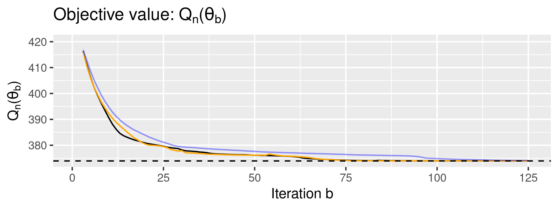
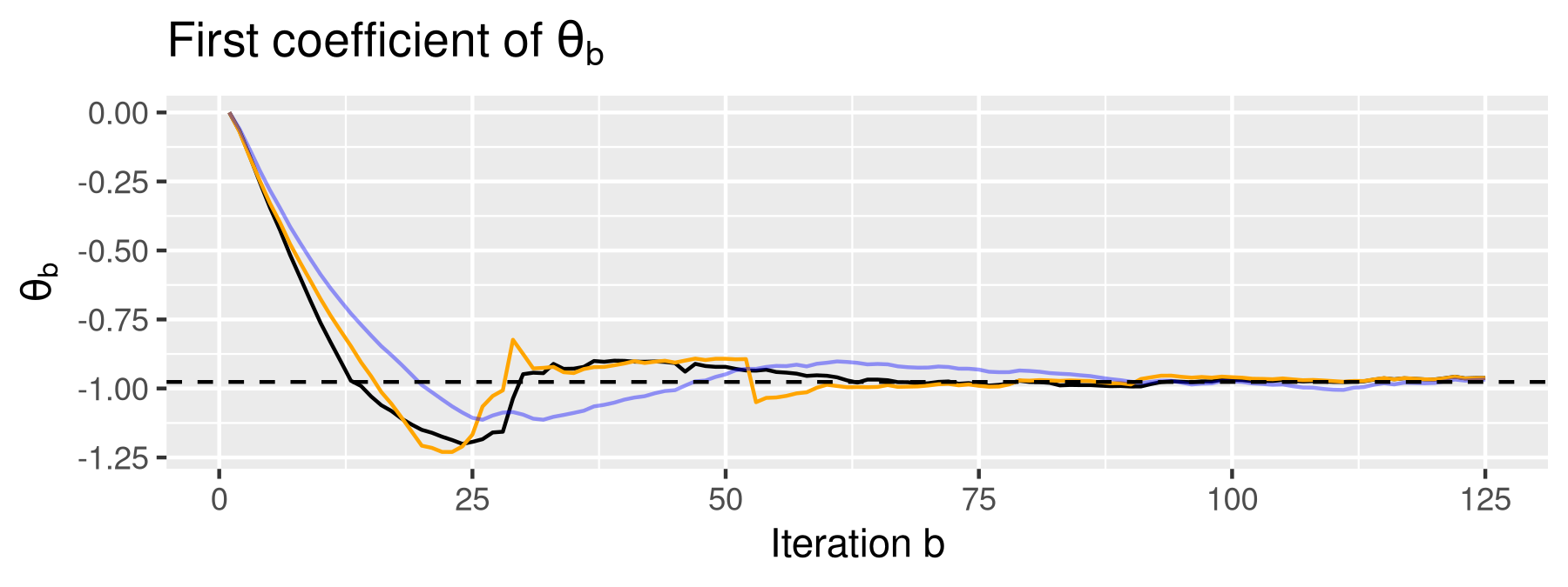
Legend: . Solid lines: black , orange , blue . Dashed black line: .
I.2 Suboptimal solutions
An important concern is when a classical optimizer converges to a point that is suboptimal, i.e. is neither a local nor a global optimum. In these cases, the user has to interve and restart an optimization at another value which can be a time-consuming process. The following illustrates, using a stylized example, the effect of the resampling noise in this scenario.
Consider a point for which the Hessian is indefinite, i.e. has both strictly positive and negative eigenvalues.55
5
See Section 3.4 Nocedal and
Wright 2006 for more details on this issue. For simplicity, the following assumes that the objective is quadratic: , with eigendecomposition , where and . There are directions with positive curvature, and directions with negative curvature. Let be the corresponding eigenvectors. Without constraints, the global minimum is attained at , , the optimizer should diverge: .
Issues with classical Newton-Raphson:
Consider the Newton-Raphson iteration , here so that: nr converges exponentially fast to the suboptimal solution . It is possible to improve the behaviour of nr by using a Hessian modification: which enforces positive definite. nr iterations are now such that:
If equals zero or is orthogonal to , then nr will converge to exponentially fast. However, nr will diverge exponentially fast if , for instance, because of the explosive root which is outside the unit circle.
The case of resampled Newton-Raphson:
The main difference between nr and rnr in this example is that rnr diverges exponentially fast with high-probability even when , which is always problematic for classical optimizers such as gd, nr, or bfgs. To simplify notation, assume that and , non-singular, and . For rnr: , which implies:
where is the same as above. Notice that follows a VAR(1) process with transition matrix which has explosive roots outside the unit circle, all equal to . Suppose which is problematic for nr. Let be the s-th row of and the -th row of , denote its variance by . For we have the AR(1) representation
Using Gaussianity and the Paley-Zygmund inequality we have the probability bound:
for any . This implies that, with high probability, diverges exponentially fast.
Numerical Illustration:
To illustrate the above numerically, consider a two-dimensional optimization problem where . We will set and vary to compare the performance of R’s bfgs optimizer, which relies on a line-search, with nr and rnr which use a fixed learning rate and the hessian modification. For , nr will converge to the saddle point and implies that nr will eventually diverge. Table I8 reports the results for a range of . Note that bfgs converges to even when . This is because, the bfgs update does not guarantee positive definiteness of the conditioning matrix so that it behaves similarly to nr without the hessian modification. nr diverges for but slowly for . As predicted, rnr diverges quickly for all .
| bfgs | nr | rnr | |||||||
|---|---|---|---|---|---|---|---|---|---|
| 0.0 | 0.00 | 0.00 | 0.00 | 0.01 | -0.01 | 0.00 | -0.01 | -90.42 | -91.35 |
| 0.1 | 0.05 | 0.05 | -0.00 | 4.78 | 5.30 | -0.25 | 5.30 | -85.65 | -81.95 |
| 0.5 | 0.23 | 0.25 | -0.00 | 23.88 | 26.53 | -6.37 | 26.53 | -66.54 | -49.47 |
| 1.0 | 0.45 | 0.50 | -0.00 | 47.76 | 53.06 | -25.48 | 53.06 | -42.66 | -20.33 |
| 5.0 | 2.26 | 2.51 | -0.06 | 238.80 | 265.32 | -637.09 | 265.32 | 148.37 | -245.96 |
Legend: bfgs: output of R’s optimizer (optim). nr and rnr: output after iterations.
True minimum is . Saddle point is .