Density Exponent Analysis: Gravity-driven steepening of the density profiles of star-forming regions
Abstract
The evolution of molecular interstellar clouds is a complex, multi-scale process. The power-law density exponent describes the steepness of density profiles, and it has been used to characterize the density structures of the clouds yet its usage is usually limited to spherically symmetric systems. Importing the Level-Set Method, we develop a new formalism that generates robust maps of a generalized density exponent at every location for complex density distributions. By applying it to high fidelity, high dynamical range map of the Perseus molecular cloud constructed using data from the Herschel and Planck satellites, we find that the density exponent exhibits a surprisingly wide range of variation (). Regions at later stages of gravitational collapse are associated with steeper density profiles. Inside a region, gas located in the vicinities of dense structures has very steep density profiles with , which forms because of depletion. This density exponent analysis reveals diverse density structures, forming a coherent picture that gravitational collapse leads to a continued steepening of the density profile. We expect our method to be effective in studying other power-law-like density structures, including granular materials and the Large-Scale Structure of the Universe.
Keywords:
ISM: clouds – ISM: structure – methods: data analysis – stars: formation – galaxies: star formation1 Introduction
Many astrophysical processes, including the gravitational collapse of molecular clouds, are complex and multi-scaled. Residing in the Galactic disk, the clouds are the nurseries of stars. They are open systems that interact with the environment constantly. Their collapses involve an interplay between turbulence (Mac Low & Klessen 2004), gravity, magnetic field (Li et al. 2014), ionization radiation, and Galactic shear, resulting in highly complex density distributions.

A clear picture of how the collapse occurs is yet to be achieved. Modern, high spatial dynamical range observations provide maps that contain an unprecedented amount of information (Zari et al. 2016). Measures like density (Probability Distribution Function) PDF (Kainulainen et al. 2009), correlation function (Padoan et al. 2003) and fractal dimension (Hetem & Lepine 1993) and spectral correlation function (Rosolowsky et al. 1999) have been proposed to quantify the structure of the star-forming regions and these are summarized in Burkhart 2021 . Despite their successes, these measures are degenerate, where original data from regions are often represented using curves where the spatial information is lost. Although the density PDF has enjoyed good success in quantifying the cloud structure and connecting simulations with observations (Kainulainen et al. 2009; Kritsuk et al. 2011; Collins et al. 2012; Li & Burkert 2016; Khullar et al. 2021), the loss of information during the compression means that the complexity of the underlying structures is often overlooked. Besides, to derive these measures, one needs to specify the boundary of a region in advance, which can be a a challenging task and efforts have been made to address the boundary issue (Li et al. 2015; Alves et al. 2015) The criteria for collapse remains an open question. Addressing the transition from clouds to clumps which hosts clustered star formation, the virial parameter (Bertoldi & McKee 1992) is often used to study whether a region should collapse or not, and gravitationally unbound clouds like the Perseus can be divided into regions which gravitationally bound by themselves (Li et al. 2015). Along this direction, (Li 2017) provides a criteria describing the transition to gravitationally-bound clumps. Analytical models have been established to describe the evolution of density structure and the star formation efficiencies in a turbulent medium (Krumholz & McKee 2005; Padoan et al. 2007; Federrath 2015; Burkhart et al. 2017; Grudić et al. 2019).
Power-law density structures such as () are common in systems that have reached intermediate asymptotic states, such that the behaviors are independent of the details of the initial and/or boundary conditions (Barenblatt 1996; Goldenfeld et al. 1989). One such example is the gravitational collapse of a molecular cloud, where stationary collapse leads to (Penston 1969; Pirogov 2009; Kritsuk et al. 2011; Girichidis et al. 2014; Naranjo-Romero et al. 2015; Murray & Chang 2015; Donkov & Stefanov 2018; Li 2018; Donkov & Stefanov 2019), and accretion flow around dense objects have (Hoyle & Lyttleton 1941; Bondi 1952). For these systems, measuring the power-law density exponent would enable us to distinguish different structures, and the value of can be directly compared against models to achieve understanding. Various attempts have been made to measure the density exponent. The most obvious approach is to fit spherical models to observational data. However, as the majority of regions we study are non-spherical, this approach is limited in practice. Another way is to derive the power-law density exponent using the density probability distribution function (PDF) (Girichidis et al. 2014; Li & Burkert 2016; Parmentier & Pasquali 2020). Although the procedure is straightforward, this statistical approach only allows for the derivation of an “effective” density exponent, which contains no information on how gas organizes spatially.
To fully exploit the diagnostics power of the density exponent , importing the Level-Set Method (LSM), we propose a new formalism to measure its value for non-spherical yet centrally condensed regions. The Level-Sets are contourlines, and the Level-Set Method is a conceptual framework where analyses of surfaces and shapes can be performed with the help of Level-Sets. By applying the LSM to state-of-the-art high dynamical range observations of star-forming regions, we obtain spatially-resolved maps of the density exponent, and reveal, for the first time, the complexity and regularity of molecular cloud structures.

2 Method
For a spherical system, the density structure can be described as where is the radius. To measure the steepness of the density profile in a given location, we adopt a local model where , and in the vicinity of , the value of can be derived as
where .
The goal is to measure the density exponent for clouds of arbitrary geometries. Assuming a 3D density structure , we divide the region using a set of densely-spaced iso-density contours, after which each subregion should be surrounded by a contour at , one or a few contours at , and it should contain values ranging from to . Assuming that the region has a volume of , inside this region, there can be a few () subregions surrounded by isosurfaces with (), and these subregions have volumes of . The size of the region can be approximated as , and the effective size of all subregions altogether can be approximated as . The Level-Set Density Exponent is
| (1) |
The procedure is illustrated in Fig. 2, and the resulting map is called the Density Exponent Map.
The advantage of the Density Exponent Analysis lies in its robustness and resolving power: the method is directly applicable to maps that contain heterogeneous structures and can be used to distinguish these structures. As an example (Fig. 2), we construct a model which contains two spherical clumps of different density profiles. We derive its density PDF and produce a density exponent map. The density PDF contains limited information since the spatial information is lost completely. In contrast, the Density Exponent Map indicates that the map should be separated into regions characterized by different density exponents and the map contain values of the density exponent at every location. The additional spatial information retrieved by the method makes it a powerful tool to analyze complex, spatially inhomogeneous datasets, such as the density structures of nearby molecular clouds. We should note that our resolved map of the density exponent is not completely identical to the density exponent derived in analytical models (Penston 1969; Pirogov 2009; Kritsuk et al. 2011; Girichidis et al. 2014; Naranjo-Romero et al. 2015; Murray & Chang 2015; Donkov & Stefanov 2018; Li 2018; Donkov & Stefanov 2019), as in those cases, the density fluctuations caused by e.g. turbulence are not accounted for.
A final remark: one can be temped to evaluate the density exponent in 2D, where
| (2) |
where represents the surface density, and derive using . However, this approach is limited, and the above-mentioned equation holds only if the structures we study are completely self-similar 11 1 https://en.wikipedia.org/wiki/Abel_transform..
3 Results & Discussions
Located at a distance of 290 pc (Zucker et al. 2018), the Perseus star-forming region is nearby and well-resolved. We use the surface density map derived using data from the Herschel and the Planck telescope (Zari et al. 2016). The original map is the opacity of dust at 870 m. We converted the map into a map of the surface density using a calibrated conversion factor provided in their Appendix. The cloud has a size of 30 pc, and the map has a resolution of 36 arcsec (). The enormous () spatial dynamical range allows detailed studies.
Derivation of the level-set density exponent requires 3D density distributions. As observations are done mostly in 2D, we develop a method (see Method Reconstruction of 3D density structure) to construct 3D density distributions using 2D maps. This is achieved by first decomposing a 2D surface density map into component maps that contain structures of different sizes and by assigning thicknesses to these component maps and combining them. For cloud-like density structures, the reconstruction allows us to measure the mass-weighted mean density exponent to an accuracy of . In our calculations, we focus on gas with . This corresponds to 40% of the gas contained in the Perseus region and the region is surrounded by a diffuse envelope that contains gas that does not contribute directly to the star formation. We also excluded unresolved regions – patches surround by contours whose sizes are smaller than 3 pixels (0.08 pc), from our analyses. To derive the density exponent map, the data is divided using 100 contour levels equally spaced in log().

In Fig. 3 we plot the density exponent distribution at the cloud center plane, which contains all the line-of-sight density maximums. ranges from -3.5 to -0.5, forming a highly inhomogeneous pattern that contains variations on different scales. We note that when the structures we study can be characterized by strict power laws, the slope of density PDF is , and the slope of the surface density PDF is . In our case, the range of translates to density PDF slopes that range from -1 to -6, and a surface density PDF slopes as shallow as -1. We note that these are very rough translations, as the derivations hold only if the underlying structures are strictly self-similar.
3.1 Inter-regional variations: Density-driven collapse
The Perseus clouds can be separated into a few pc-sized subregions. Each region has a corresponding gravitational potential dip (Li et al. 2015), and these regions can collapse to form star clusters or associations. We first divide the cloud into these regions and evaluate parameters including the mass-weighed mean density exponent and the mean densities. We also characterize these regions by deriving a quantify called the dense gas fraction (see Methods Measurement of dense gas fraction and star formation activity). Since all the dense gas would collapse to form individual or multiple stars, the dense gas mass fraction is a direct indicator of the star formation activity.
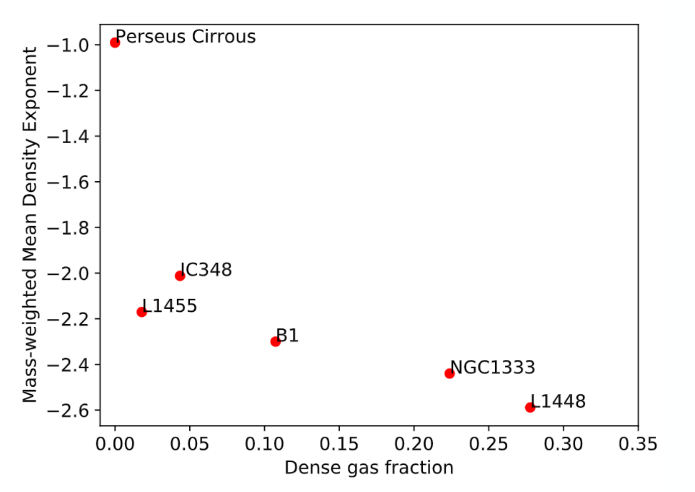
Correlations between these quantities are summarized in the right panel of Fig. 3. In general, regions of steeper density profiles have higher dense gas mass fractions. Thus, the formation of dense gas, which occurs on tiny scales, is deeply linked to a global steepening of the density profile. Although the link between dense gas mass fractions and the steepness of the density profile inferred from the shape of the surface density PDF is somehow established (Stutz & Kainulainen 2015; Li & Burkert 2016), our maps provide a more detailed view, where steepening occurs at the high-density regions found around the dense cores.
By plotting the mass-weighted density exponent
| (3) |
against the mean density (Fig. 3), we find that regions of higher densities tend to have steeper density profiles, which suggests a density-driven collapse scenario. Since all regions belong to the Perseus molecular cloud, we assume that they have almost the same age . Provided that they evolve at paces set by their free-fall time , which is related to the mean densities by , the evolutionary stage can be parameterized using . Regions with larger are more evolved, have higher densities when observed (higher ), with steeper density profiles and higher dense gas fraction. In reality, due to the presence of turbulence, the actual collapse time can be a few times the collapse (Li 2018; Appel et al. 2022). But this additional factor will not change our conclusion. The picture of a steepening density profile is consistent with results from a recent paper (Gómez et al. 2020), and the correlations point to a simple picture where the mean gas density sets the pace at which a region evolves, leading to the steepening of the density profile 22 2 One might be worried about the effect of protostellar outflows (Bally 2016). Indeed, regions like the NGC1333 (Knee & Sandell 2000) contain a number of these. However, the effects should not be significant, as recent simulations found that outflows lead to an excess of low-density gas which we do not analyze (Appel et al. 2022). .
The map also allows us to identify a new region called “Perseus Cirrous" (Fig. 3) for the first time. Although overlooked by previous studies, the region stands out in our analyses due to its shallow density profile (). The region occupies the shallow end of the density exponent parameter space and its structure should be representative of the structure gas at the early stages of gravitational collapse. On the other hand, since this region has a density profile that is significantly shallower than those the others, it is possible that this region belongs to the gravitationally unbound phase, whereas others belong to the bound phase, as suggested by previous studies (Kritsuk et al. 2007; Collins et al. 2012; Li 2017).
3.2 Summary & Future Extensions
The evolution of molecular clouds is exemplary of complex, multi-scale processes. Regions in molecular clouds appear to be gravitationally bound at pc scale (Li et al. 2015), and the collapse of dense cores, which is directly related to star formation, occurs at 0.05 pc. Importing the Level-Set Method, we develop a new, robust formalism to compute spatially resolved maps of the density exponent. On the pc scale, the mass-weighted mean density exponent correlates with the star formation activity. On smaller scales ( 1 pc), the density exponent still exhibits significant variations. This complex pattern results from a continued steepening of the density profile driven by gravitational collapse.
The spatial information our method provides is valuable for large, inhomogeneous datasets. The Level Set-based formalism can be modified to suit different models, for example, to derive the scale length for exponential-like structures, which we will explore in the future. We expect our method to be effective for other structures including the density structure of granular materials and the Large-Scale Structure of the Universe.
One limitation of our method is that it still requires 3D density. In the current approach, we are using 3D density distribution constructed from 2D surface density maps. For non-self-similar structures, the relation between exponent evaluated in 2D and 3D are not trivial 33 3 This has been well-understood under the Abel Transform https://en.wikipedia.org/wiki/Abel_transform., and our ongoing studies (Li & Zhou in prep) suggest that compared to the current approach, evaluating the density exponent from 2D is less accurate but significantly easier to implement, making widespread applications feasible. These will be explored in our future papers.
Acknowledgements
We thank the referee for a careful reading of the paper and for the comments. GXL acknowledges supports from NSFC grant W820301904 and 12033005.
Data availability
The data this publication makes use of is publicly available, the link can be found in Zari et al. 2016, and we use code is from Li 2022, which is available at https://gxli.github.io/Constrained-Diffusion-Decomposition/.
References
- Alves et al. (2015) Alves J., Lombardi M., Lada C., 2015, in IAU General Assembly. p. 2253648
- Appel et al. (2022) Appel S. M., Burkhart B., Semenov V. A., Federrath C., Rosen A. L., 2022, ApJ, 927, 75
- Bally (2016) Bally J., 2016, ARA&A, 54, 491
- Barenblatt (1996) Barenblatt G. I., 1996, Scaling, Self-similarity, and Intermediate Asymptotics
- Bertoldi & McKee (1992) Bertoldi F., McKee C. F., 1992, ApJ, 395, 140
- Bondi (1952) Bondi H., 1952, MNRAS, 112, 195
- Burkhart (2021) Burkhart B., 2021, PASP, 133, 102001
- Burkhart et al. (2017) Burkhart B., Stalpes K., Collins D. C., 2017, ApJ, 834, L1
- Clark et al. (2019) Clark P. C., Glover S. C. O., Ragan S. E., Duarte-Cabral A., 2019, MNRAS, 486, 4622
- Collins et al. (2012) Collins D. C., Kritsuk A. G., Padoan P., Li H., Xu H., Ustyugov S. D., Norman M. L., 2012, ApJ, 750, 13
- Donkov & Stefanov (2018) Donkov S., Stefanov I. Z., 2018, MNRAS, 474, 5588
- Donkov & Stefanov (2019) Donkov S., Stefanov I., 2019, MNRAS, 485, 3224
- Enoch et al. (2006) Enoch M. L., et al., 2006, ApJ, 638, 293
- Federrath (2015) Federrath C., 2015, MNRAS, 450, 4035
- Girichidis et al. (2014) Girichidis P., Konstandin L., Whitworth A. P., Klessen R. S., 2014, ApJ, 781, 91
- Goldenfeld et al. (1989) Goldenfeld N., Martin O., Oono Y., 1989, Journal of Scientific Computing, 4, 355
- Gómez et al. (2020) Gómez G. C., Vázquez-Semadeni E., Palau A., 2020, arXiv e-prints, p. arXiv:2009.14151
- Grudić et al. (2019) Grudić M. Y., Hopkins P. F., Lee E. J., Murray N., Faucher-Giguère C.-A., Johnson L. C., 2019, MNRAS, 488, 1501
- Hetem & Lepine (1993) Hetem A. J., Lepine J. R. D., 1993, A&A, 270, 451
- Hoyle & Lyttleton (1941) Hoyle F., Lyttleton R. A., 1941, MNRAS, 101, 227
- Kainulainen et al. (2009) Kainulainen J., Beuther H., Henning T., Plume R., 2009, A&A, 508, L35
- Kauffmann et al. (2008) Kauffmann J., Bertoldi F., Bourke T. L., Evans N. J. I., Lee C. W., 2008, A&A, 487, 993
- Khullar et al. (2021) Khullar S., Federrath C., Krumholz M. R., Matzner C. D., 2021, MNRAS, 507, 4335
- Knee & Sandell (2000) Knee L. B. G., Sandell G., 2000, A&A, 361, 671
- Kritsuk et al. (2007) Kritsuk A. G., Norman M. L., Padoan P., Wagner R., 2007, ApJ, 665, 416
- Kritsuk et al. (2011) Kritsuk A. G., Norman M. L., Wagner R., 2011, ApJ, 727, L20
- Krumholz & McKee (2005) Krumholz M. R., McKee C. F., 2005, ApJ, 630, 250
- Li (2017) Li G.-X., 2017, MNRAS, 465, 667
- Li (2018) Li G.-X., 2018, MNRAS, 477, 4951
- Li (2022) Li G.-X., 2022, arXiv e-prints, p. arXiv:2201.05484
- Li & Burkert (2016) Li G.-X., Burkert A., 2016, MNRAS, 461, 3027
- Li et al. (2014) Li H. B., Goodman A., Sridharan T. K., Houde M., Li Z. Y., Novak G., Tang K. S., 2014, in Beuther H., Klessen R. S., Dullemond C. P., Henning T., eds, Protostars and Planets VI. p. 101 (arXiv:1404.2024), doi:10.2458/azu_uapress_9780816531240-ch005
- Li et al. (2015) Li G.-X., Wyrowski F., Menten K., Megeath T., Shi X., 2015, A&A, 578, A97
- Li et al. (2016) Li G.-X., Urquhart J. S., Leurini S., Csengeri T., Wyrowski F., Menten K. M., Schuller F., 2016, A&A, 591, A5
- Mac Low & Klessen (2004) Mac Low M.-M., Klessen R. S., 2004, Reviews of Modern Physics, 76, 125
- Murray & Chang (2015) Murray N., Chang P., 2015, ApJ, 804, 44
- Naranjo-Romero et al. (2015) Naranjo-Romero R., Vázquez-Semadeni E., Loughnane R. M., 2015, ApJ, 814, 48
- Padoan et al. (2003) Padoan P., Goodman A. A., Juvela M., 2003, ApJ, 588, 881
- Padoan et al. (2007) Padoan P., Nordlund Å., Kritsuk A. G., Norman M. L., Li P. S., 2007, ApJ, 661, 972
- Parmentier & Pasquali (2020) Parmentier G., Pasquali A., 2020, ApJ, 903, 56
- Penston (1969) Penston M. V., 1969, MNRAS, 144, 425
- Pirogov (2009) Pirogov L. E., 2009, Astronomy Reports, 53, 1127
- Rosolowsky et al. (1999) Rosolowsky E. W., Goodman A. A., Wilner D. J., Williams J. P., 1999, ApJ, 524, 887
- Stutz & Kainulainen (2015) Stutz A. M., Kainulainen J., 2015, A&A, 577, L6
- Zari et al. (2016) Zari E., Lombardi M., Alves J., Lada C. J., Bouy H., 2016, A&A, 587, A106
- Zucker et al. (2018) Zucker C., Schlafly E. F., Speagle J. S., Green G. M., Portillo S. K. N., Finkbeiner D. P., Goodman A. A., 2018, ApJ, 869, 83
Reconstruction of 3D density structure
We develop a formalism to construct 3D density structures from 2D observations.ð The reconstruction consists of two steps. First, using a method called “constrained diffusion decomposition” (Li 2022) , we decompose the surface density maps into component maps that contain structures of different sizes. The first of these maps contain structures whose sizes range from 1 to 2 pixels, and the th of these maps contain structures of sizes between and pixels. Second, a 3D density structure is constructed using the component maps. During our reconstruction, the channels are assumed to be slabs of different thicknesses, where and along the line of sight, the th channel has a Gaussian density profile of dispersion of pixels. The final 3D density structure is assumed to be the sum of these slabs. When combining these slabs, we aligned them such that the density maximums stay on the same plane.
Due to the lack of information on the distribution of gas along the line of sight direction, the density structure we constructed is not identical to but resembles the real one. We first test our method by producing a 3D clump of where , projected it to 2D and verified that our reconstruction allows us to recover the density exponent to an accuracy of . Then, using results from numerical simulations (Clark et al. 2019), we perform density exponent analysis on both the original data and the 3D data constructed from a 2D projection. They simulated the collapse of a 1000 clump, with a sophisticated treatment of the chemistry and thermal physics of the ISM. The initial condition resembles regions that resemble the clumps found in Perseus. The simulation produced a density structure that is sufficiently complex, which enables us to test the robustness of our method.
We limit ourselves to gas with and find that the reconstructed cloud and the original cloud are similar in terms of (Fig. 4). The original cloud has a mass-weighted density exponent of -1.66, and the reconstructed cloud has . The difference is noticeable but is still small compared to the variations we are interested in. Although some small-scale details are lost, compared to the original cloud, the reconstructed cloud has very similar density exponent distributions.

Measurement of dense gas fraction and star formation activity
The star formation activity is characterized by the dense gas ratio – the ratio between the amount of the dense gas which should collapse to form stars and the total amount of gas in a region. To trace the dense gas, we use the 870m observation towards the Perseus region where only dense gas can be observed (Enoch et al. 2006), and created a mask containing significant () detections, which correspond to a surface density of (Converted from a limiting sensativity of , using the values Kauffmann et al. 2008, and this observations a 5- mass-limit of 0.18 ). Using the Herschel-Planck surface density map (Zari et al. 2016), the total amount of gas is derived by integrating over whole regions, and the amount of dense gas is derived by integrating over subregions with significant Bolocam 870m detections.
Relation between density exponent, surface density exponent and density power-law
Following previous papers (Kritsuk et al. 2011; Girichidis et al. 2014; Li et al. 2016), assuming a sphere whose density is
| (4) |
where , the (volume-weighted) density distribution is
| (5) |
Thus
| (6) |
where the slope density PDF is .
The corresponding surface density distribution is
| (7) |
thus
| (8) |
and
| (9) |
where the slope is .
Relation between density exponent and dense gas fraction
In Fig. 5 we plot the relation between density exponent and dense gas fraction.