State Estimation Methods
for Continuous-Discrete Nonlinear Systems
involving Stochastic Differential Equations

Marcus Krogh Nielsen, Tobias K. S. Ritschel, Ib Christensen, Jess Dragheim Jakob Kjøbsted Huusom Krist V. Gernaey John Bagterp Jørgensen Thanks: $ˆ*$This work is funded by Innovation Fund Denmark (9065-00269B). Marcus Krogh Nielsen, Tobias K. S. Ritschel, and John Bagterp Jørgensen are with the Department of Applied Mathematics and Computer Science, and Jakob Kjøbsted Huusom og Krist V. Gernaey are with the Department of Chemical and Biochemical Engineering, Technical University of Denmark, DK-2800 Kgs. Lyngby, Denmark. Marcus Krogh Nielsen, Jess Dragheim, and Ib Christensen are with Unibio A/S, DK-4000 Roskilde, Denmark. email: {mkrni,jbjo}@dtu.dk Thanks:

Abstract

In this work, we present methods for state estimation in continuous-discrete nonlinear systems involving stochastic differential equations. We present the extended Kalman filter, the unscented Kalman filter, the ensemble Kalman filter, and a particle filter. We implement the state estimation methods in Matlab. We evaluate the performance of the methods on a simulation of the modified four-tank system. We implement the state estimation methods for non-stiff systems, i.e., using an explicit numerical integration scheme. The implementation of the extended Kalman filter utilises the Joseph stabilising form for numerical stability. We evaluate the accuracy of the state estimation methods in terms of the mean absolute percentage error over the simulation horizon. We show that each method successfully estimates the states and unmeasured disturbances of the simulated modified four-tank system. Finally, we present conclusions.

I Introduction

State estimation is widely applied in industry, e.g., for monitoring, fault-detection, and model-based control. The objective of state estimation is to predict and reconstruct the states of a mathematical model using measurements from a physical system. The Kalman filter provides optimal estimates for systems with Gaussian process and measurement noise, but is limited to system with linear dynamics [1]. For nonlinear systems, the exact evolution of the state distribution can be computed as the solution to the Fokker-Planck equation (Kolmogorov’s forward equation). However, the Fokker-Planck equation is a partial differential equation where the number of dimensions equal the number of states in the system. The Fokker-Planck equation suffers from the curse of dimensionality and solving it is therefore impractical for systems with more than a few states [2]. This paper describes four approximate methods for state estimation, 1) the extended Kalman filter (EKF), 2) the unscented Kalman filter (UKF), 3) the ensemble Kalman filter (EnKF), and 4) a particle filter (PF).

In the EKF, the equations of the original Kalman filter are applied on a local linearisation of a nonlinear system [3]. The EKF is a computationally efficient method, but the quality of the estimates depend on the nonlinearity of the system [4]. Additionally, some stability issues may arise in relation to fixed step-size solutions. This and more has been addressed in other works [5, 6, 7]. In the UKF, an unscented transformation is used as an approximation for the first two moments of the true nonlinear distribution. The unscented transformation is propagated through the nonlinear dynamics and each sigma-point is updated using observations from the physical system [8]. For some systems, the UKF has shown higher accuracy than the EKF, while still being computationally efficient [9]. However, the UKF also suffers from inaccuracy in highly nonlinear systems. For the UKF, some of the issues pertaining to nonlinearity and numerical instability have been addressed in more recent contributions [10, 11, 12, 13]. In the EnKF, a set of particles, the ensemble, is randomly sampled from the state distribution and propagated through the nonlinear system dynamics. Each particle in the ensemble is updated separately using the Kalman filter update when a measurement becomes available. The state estimates are computed statistically from the ensembles [14, 15, 16]. In PFs, a set of particles is sampled from the state distribution and propagated through the nonlinear system dynamics. When a measurement becomes available, the particles are resampled in accordance with their likelihood of being observed. The likelihoods are computed using the innovation posterior distribution. Similarly to the EnKF, the state estimates are determined statistically from the particles [17, 18, 19, 20]. The EKF and UKF provide efficient state estimation, but suffers from loss of accuracy for highly nonlinear systems. The EnKF and PFs provide a set of sampled particles from the true nonlinear distribution, but their computational efficiency depends on the number of particles required for the estimates to reach the desired accuracy. As a result of this, the EnKF and PF can be computationally inefficient for high dimensional systems.

The aim of this paper is to provide a condensed overview of available methods for state estimation in nonlinear systems. The intention is to further the diversification in application of different state estimation methods within a wider range of industries - utilising the best available tool for a particular task. The nonlinear state estimation methods can generally be separated into two steps; prediction and filtering. In the prediction step (time update), the system is propagated through time based on past information from a physical system. In the filtering step (measurement update), the state estimates are updated with the latest measurement information.

The paper is structured as follows. In Section II, we present the nonlinear continuous-discrete stochastic differential equation models used in simulation and state estimation. In Section III, we present the EKF, the UKF, the EnKF, and a PF, and finally present a discussion of the methods. In Section IV, we present a numerical example of state estimation for a modified four-tank system. Finally, we present conclusions in Section V.

II Nonlinear Continuous-Discrete Stochastic Differential Equation Models

We consider continuous-discrete systems, in which the system state is described by nonlinear continuous stochastic differential equations and measurements are taken at discrete points in time. The nonlinear continuous-discrete stochastic differential equation models are defined as


$\displaystyle\begin{split}d\boldsymbol{x}(t)&=f(t,\boldsymbol{x}(t),u(t),d(t),\theta)dt\\ &+\sigma(t,\boldsymbol{x}(t),u(t),d(t),\theta)d\boldsymbol{\omega}(t),\end{split}$		(1a)
$\displaystyle\boldsymbol{y}(t_{k})$	$\displaystyle=h(t_{k},\boldsymbol{x}(t_{k}),\theta)+\boldsymbol{v}(t_{k}),$	(1b)

where $f(\cdot)$ is the drift function, $\sigma(\cdot)$ is the diffusion function, and $h(\cdot)$ is the measurement function. The states are $\boldsymbol{x}(t)\in\mathbb{R}^{n_{x}}$ , the inputs are $u(t)\in\mathbb{R}^{n_{u}}$ , the disturbances are $d(t)\in\mathbb{R}^{n_{d}}$ , the parameters are $\theta\in\mathbb{R}^{n_{\theta}}$ , and the measurements are $\boldsymbol{y}(t_{k})\in\mathbb{R}^{n_{y}}$ . The process noise $\boldsymbol{\omega}(t)\in\mathbb{R}^{n_{\omega}}$ is a standard Weiner process, such that $d\boldsymbol{\omega}(t)\sim\mathcal{N}\left(0,Idt\right)$ , and $\boldsymbol{v}(t_{k})\sim\mathcal{N}\left(0,R\right)$ is the measurement noise. For simplicity, the initial state is assumed to be known and to be distributed as

\displaystyle\boldsymbol{x}_{0}

\displaystyle\sim\mathcal{N}\left(\bar{\boldsymbol{x}}_{0},P_{0}\right).

(2)

III State Estimation in Nonlinear Systems

In this section, we present methods for state estimation in continuous-discrete nonlinear systems following (1).

III-A Continuous-discrete extended Kalman filter

The EKF is initialised with the mean and covariance of the initial state of the system described in (2)


$\displaystyle\hat{x}_{0\|0}$	$\displaystyle=\bar{x}_{0},$	(3a)
$\displaystyle P_{0\|0}$	$\displaystyle=P_{0}.$	(3b)

III-A1 Time update

In the time update, the mean and covariance are computed as the solution to the ordinary differential equations (ODEs) for $t\in\left[t_{k},t_{k+1}\right]$


$\displaystyle\frac{d\hat{x}_{k}(t)}{dt}$	$\displaystyle=f(t,\hat{x}_{k}(t),u(t),d(t),\theta),$	(4a)
$\displaystyle\frac{dP_{k}(t)}{dt}$	$\displaystyle=A_{k}(t)P_{k}(t)+P_{k}(t)A_{k}^{T}(t)+\sigma_{k}(t)\sigma_{k}^{T}(t),$	(4b)

where $\hat{x}_{k}(t_{k})=\hat{x}_{k|k}$ , and $P_{k}(t_{k})=P_{k|k}$ . $A_{k}(t)=\frac{\partial f}{\partial x}(t,\hat{x}_{k}(t),u(t),d(t),\theta)$ and $\sigma_{k}(t)=\sigma(t,\hat{x}_{k}(t),u(t),d(t),\theta)$ . Alternatively, the covariance update can be represented and solved on integral form as presented by [21]. The mean and covariance estimates are


$\displaystyle\hat{x}_{k+1\|k}$	$\displaystyle=\hat{x}_{k}(t_{k+1}),$	(5a)
$\displaystyle P_{k+1\|k}$	$\displaystyle=P_{k}(t_{k+1}).$	(5b)

III-A2 Measurement update

In the measurement update, we compute the innovation and its covariance as


$\displaystyle e_{k}$	$\displaystyle=y_{k}-\hat{y}_{k\|k-1},$	(6a)
$\displaystyle R_{e,k}$	$\displaystyle=C_{k}P_{k\|k-1}C_{k}^{T}+R,$	(6b)

where


$\displaystyle\hat{y}_{k\|k-1}$	$\displaystyle=h(t_{k},\hat{x}_{k\|k-1},\theta),$	(7a)
$\displaystyle C_{k}$	$\displaystyle=\frac{\partial h}{\partial x}(t_{k},\hat{x}_{k\|k-1},\theta).$	(7b)

The Kalman gain is computed as

\displaystyle\begin{split}K_{f_{x},k}&=P_{k|k-1}C_{k}^{T}R_{e,k}^{-1}.\end{split}

(8)

The mean and covariance estimates are computed as


$\displaystyle\hat{x}_{k\|k}$	$\displaystyle=\hat{x}_{k\|k-1}+K_{f_{x},k}e_{k},$	(9a)
$\displaystyle P_{k\|k}$	$\displaystyle=P_{k\|k-1}-K_{f_{x},k}R_{e,k}K_{f_{x},k}^{T}$	(9b)
$\displaystyle\begin{split}&=\left(I-K_{f_{x},k}C_{k}\right)P_{k\|k-1}\left(I-K_{f_{x},k}C_{k}\right)^{T}\\ &+K_{f_{x},k}RK_{f_{x},k}^{T},\end{split}$		(9c)

where (9c), Joseph stabilising form, is numerically stable.

III-B Continuous-discrete unscented Kalman filter

The unscented Kalman filter is initialised with the mean and covariance of the initial state of the system described in (2)


$\displaystyle\hat{x}_{0\|0}$	$\displaystyle=\bar{x}_{0},$	(10a)
$\displaystyle P_{0\|0}$	$\displaystyle=P_{0}.$	(10b)

III-B1 Time update

In the time update, we compute the parameters


$\displaystyle\bar{c}$	$\displaystyle=\alpha^{2}\left(\bar{n}+\kappa\right),$	(11a)
$\displaystyle\bar{\lambda}$	$\displaystyle=\alpha^{2}\left(\bar{n}+\kappa\right)-\bar{n},$	(11b)

where $\alpha\in]0,1]$ , $\kappa\in\left[0,\infty\right[$ , and $\bar{n}=n_{x}+n_{\omega}$ . We compute the sigma-point weights


$\displaystyle\bar{W}_{m}^{(0)}$	$\displaystyle=\frac{\bar{\lambda}}{\bar{n}+\bar{\lambda}},$	(12a)
$\displaystyle\bar{W}_{c}^{(0)}$	$\displaystyle=\frac{\bar{\lambda}}{\bar{n}+\bar{\lambda}}+1-\alpha^{2}+\beta,$	(12b)
$\displaystyle\bar{W}_{m}^{(i)}$	$\displaystyle=\bar{W}_{c}^{(i)}=\frac{1}{2\left(\bar{n}+\bar{\lambda}\right)},$	(12c)

for $i\in\{1,2,\dots,2\bar{n}\}$ and where $\beta\in\left[0,\infty\right[$ ( $\beta=2$ optimal for Gaussian distributions). We sample deterministically a set of $2\bar{n}+1$ sigma-points. For propagation through the deterministic dynamics (ODE), we compute $2n_{x}+1$ sigma-points


$\displaystyle\hat{x}_{k\|k}^{(0)}$	$\displaystyle=\hat{x}_{k\|k},$	(13a)
$\displaystyle\hat{x}_{k\|k}^{(i)}$	$\displaystyle=\hat{x}_{k\|k}+\sqrt{\bar{c}}\left(\sqrt{P_{k\|k}}\right)_{i},$	(13b)
$\displaystyle\hat{x}_{k\|k}^{(n_{x}+i)}$	$\displaystyle=\hat{x}_{k\|k}-\sqrt{\bar{c}}\left(\sqrt{P_{k\|k}}\right)_{i},$	(13c)

for $i\in\{1,2,\dots,n_{x}\}$ . $\left(\sqrt{P_{k|k}}\right)_{i}$ denotes the $i$ ’th column of the Cholesky decomposition of the covariance. For propagation through the stochastic dynamics, we compute $2n_{\omega}$ sigma-points

\displaystyle\hat{x}_{k|k}^{(2n_{x}+i)}

\displaystyle=\hat{x}_{k|k},

(14)

for $i\in\{1,2,\dots,2n_{\omega}\}$ . Additionally, we compute the process noise


$\displaystyle d\omega_{k}^{(2n_{x}+i)}(t)$	$\displaystyle=\sqrt{\bar{c}~dt}\left(I\right)_{i},$	(15a)
$\displaystyle d\omega_{k}^{(2n_{x}+n_{\omega}+i)}(t)$	$\displaystyle=-\sqrt{\bar{c}~dt}\left(I\right)_{i},$	(15b)

where $i\in\{1,2,\dots,n_{\omega}\}$ . We propagate the first sigma-points through the deterministic dynamics for $t\in\left[t_{k},t_{k+1}\right]$ and compute the predictions as the solution to

\displaystyle d\hat{x}_{k}^{(i)}(t)

\displaystyle=f(t,\hat{x}_{k}^{(i)}(t),u(t),d(t),\theta)dt,

(16)

for $\hat{x}_{k}^{(i)}(t_{k})=\hat{x}_{k|k}^{(i)}$ and $i\in\{0,1,\dots,2n_{x}\}$ . We similarly propagate the remaining sigma-points through the stochastic dynamics for $t\in\left[t_{k},t_{k+1}\right]$ and compute the predictions as the solution to

\displaystyle\begin{split}d\hat{x}_{k}^{(i)}(t)&=f(t,\hat{x}_{k}^{(i)}(t),u(t),d(t),\theta)dt\\ &+\sigma(t,\hat{x}_{k}^{(i)}(t),u(t),d(t),\theta)d\omega_{k}^{(i)}(t),\end{split}

(17)

where $\hat{x}_{k}^{(i)}(t_{k})=\hat{x}_{k|k}^{(i)}$ and $i\in\{2n_{x}+1,2n_{x}+2,\dots,2n_{x}+2n_{\omega}\}$ . The predictions are computed as the solution to (16) and (17), as

\displaystyle\hat{x}_{k+1|k}^{(i)}

\displaystyle=\hat{x}_{k}^{(i)}(t_{k+1}).

(18)

The mean and covariance estimates are computed as


$\displaystyle\hat{x}_{k+1\|k}$	$\displaystyle=\sum_{i=0}^{2\bar{n}}\bar{W}_{m}^{(i)}\hat{x}_{k+1\|k}^{(i)},$	(19a)
$\displaystyle P_{k+1\|k}$	$\displaystyle=\sum_{i=0}^{2\bar{n}}\bar{W}_{c}^{(i)}\left(\hat{x}_{k+1\|k}^{(i)}-\hat{x}_{k+1\|k}\right)\left(\hat{x}_{k+1\|k}^{(i)}-\hat{x}_{k+1\|k}\right)^{T}.$	(19b)

III-B2 Measurement update

In the measurement update, we compute the parameters


$\displaystyle c$	$\displaystyle=\alpha^{2}\left(n_{x}+\kappa\right),$	(20a)
$\displaystyle\lambda$	$\displaystyle=\alpha^{2}\left(n_{x}+\kappa\right)-n_{x}.$	(20b)

We compute the sigma-point weights


$\displaystyle W_{m}^{(0)}$	$\displaystyle=\frac{\lambda}{n_{x}+\lambda},$	(21a)
$\displaystyle W_{c}^{(0)}$	$\displaystyle=\frac{\lambda}{n_{x}+\lambda}+1-\alpha^{2}+\beta,$	(21b)
$\displaystyle W_{m}^{(i)}$	$\displaystyle=W_{c}^{(i)}=\frac{1}{2\left(n_{x}+\lambda\right)},$	(21c)

for $i\in\{1,2,\dots,2n_{x}\}$ . We compute a set of $2n_{x}+1$ deterministically sampled sigma-points


$\displaystyle\hat{x}_{k\|k-1}^{(0)}$	$\displaystyle=\hat{x}_{k\|k-1},$	(22a)
$\displaystyle\hat{x}_{k\|k-1}^{(i)}$	$\displaystyle=\hat{x}_{k\|k-1}+\sqrt{c}\left(\sqrt{P_{k\|k-1}}\right)_{i},$	(22b)
$\displaystyle\hat{x}_{k\|k-1}^{(n_{x}+i)}$	$\displaystyle=\hat{x}_{k\|k-1}-\sqrt{c}\left(\sqrt{P_{k\|k-1}}\right)_{i},$	(22c)

for $i\in\{1,2,\dots,n_{x}\}$ . We compute the innovation as

\displaystyle e_{k}

\displaystyle=y_{k}-\hat{y}_{k|k-1},

(23)

where the prediction of the measurement prediction is computed as

\displaystyle\hat{y}_{k|k-1}

\displaystyle=\hat{z}_{k|k-1}=\sum_{i=0}^{2n_{x}}W_{m}^{(i)}\hat{z}_{k|k-1}^{(i)},

(24)

for $\hat{z}_{k|k-1}^{(i)}=h(t_{k},\hat{x}_{k|k-1}^{(i)},\theta)$ . We compute the covariance and cross-covariance information from the sigma-points


$\displaystyle R_{zz,k\|k-1}$	$\displaystyle=\sum_{i=0}^{2n_{x}}W_{c}^{(i)}\left(\hat{z}_{k\|k-1}^{(i)}-\hat{z}_{k\|k-1}\right)\left(\hat{z}_{k\|k-1}^{(i)}-\hat{z}_{k\|k-1}\right)^{T},$	(25a)
$\displaystyle R_{e,k}$	$\displaystyle=R_{yy,k\|k-1}=R_{zz,k\|k-1}+R,$	(25b)
$\displaystyle R_{xy,k\|k-1}$	$\displaystyle=\sum_{i=0}^{2n_{x}}W_{c}^{(i)}\left(\hat{x}_{k\|k-1}^{(i)}-\hat{x}_{k\|k-1}\right)\left(\hat{z}_{k\|k-1}^{(i)}-\hat{z}_{k\|k-1}\right)^{T}.$	(25c)

The Kalman gain is computed as

\displaystyle K_{f_{x},k}

\displaystyle=R_{xy,k|k-1}R_{e,k}^{-1}.

(26)

The mean and covariance estimates are computed as


$\displaystyle\hat{x}_{k\|k}$	$\displaystyle=\hat{x}_{k\|k-1}+K_{f_{x},k}e_{k},$	(27a)
$\displaystyle P_{k\|k}$	$\displaystyle=P_{k\|k-1}-K_{f_{x},k}R_{e,k}K_{f_{x},k}^{T}.$	(27b)

III-C Continuous-discrete ensemble Kalman filter

The ensemble Kalman filter is initialised with a set of particles, the ensemble, sampled from the initial state distribution from (2). The initial state ensemble is denoted

\displaystyle\{\hat{x}_{0|0}^{(i)}\}_{i=1}^{N_{p}}.

(28)

III-C1 Time update

In the time update, each particle in the ensemble is propagated through the system dynamics. The prediction ensemble is computed as the solution to

\displaystyle\begin{split}d\boldsymbol{x}_{k}^{(i)}(t)&=f(t,\boldsymbol{x}_{k}^{(i)}(t),u(t),d(t),\theta)dt\\ &+\sigma(t,\boldsymbol{x}_{k}^{(i)}(t),u(t),d(t),\theta)d\boldsymbol{\omega}_{k}(t),\end{split}

(29)

for $i\in\{1,2,\dots,N_{p}\}$ and $t\in\left[t_{k},t_{k+1}\right]$ . The initial value is $x_{k}^{(i)}=\hat{x}_{k|k}^{(i)}$ . The set of solutions, $\hat{x}_{k+1|k}^{(i)}=x_{k}^{(i)}(t_{k+1})$ , gives rise to the prediction ensemble

\displaystyle\{\hat{x}_{k+1|k}^{(i)}\}_{i=1}^{N_{p}}.

(30)

The mean and covariance estimates are computed as


$\displaystyle\hat{x}_{k+1\|k}$	$\displaystyle=\frac{1}{N_{p}}\sum_{i=1}^{N_{p}}\hat{x}_{k+1\|k}^{(i)},$	(31a)
$\displaystyle P_{k+1\|k}$	$\displaystyle=\frac{1}{N_{p}-1}\sum_{i=1}^{N_{p}}\left(\hat{x}_{k+1\|k}^{(i)}-\hat{x}_{k+1\|k}\right)\left(\hat{x}_{k+1\|k}^{(i)}-\hat{x}_{k+1\|k}\right)^{T}.$	(31b)

III-C2 Measurement update

In the measurement update, we compute the ensemble of predictions, $\{\hat{z}_{k|k-1}^{(i)}\}_{i=1}^{N_{p}}$ , where

\displaystyle z_{k|k-1}^{(i)}

\displaystyle=h(t_{k},\hat{x}_{k|k-1}^{(i)},\theta),

(32)

for $i\in\{1,2,\dots,N_{p}\}$ . Furthermore, we compute the mean and covariance of the measurement distribution and cross-covariance of states and measurements, as


$\displaystyle\hat{y}_{k\|k-1}$	$\displaystyle=\hat{z}_{k\|k-1}=\frac{1}{N_{p}}\sum_{i=1}^{N_{p}}\hat{z}_{k\|k-1}^{(i)},$	(33a)
$\displaystyle R_{zz,k\|k-1}$	$\displaystyle=\frac{1}{N_{p}-1}\sum_{i=1}^{N_{p}}\left(\hat{z}_{k\|k-1}^{(i)}-\hat{z}_{k\|k-1}\right)\left(\hat{z}_{k\|k-1}^{(i)}-\hat{z}_{k\|k-1}\right)^{T},$	(33b)
$\displaystyle R_{yy,k\|k-1}$	$\displaystyle=R_{zz,k\|k-1}+R,$	(33c)
$\displaystyle R_{xy,k\|k-1}$	$\displaystyle=\frac{1}{N_{p}-1}\sum_{i=1}^{N_{p}}\left(\hat{x}_{k\|k-1}^{(i)}-\hat{x}_{k\|k-1}\right)\left(\hat{y}_{k\|k-1}^{(i)}-\hat{y}_{k\|k-1}\right)^{T},$	(33d)

and we compute samples from measurement distribution, as

\displaystyle y_{k}^{(i)}

\displaystyle=y_{k}+v_{k}^{(i)},

(34)

where $v_{k}^{(i)}$ are realisations of the measurement noise, $\boldsymbol{v}_{k}\sim\mathcal{N}(0,R)$ . The innovations are computed for each particle in the measurement ensemble, as

\displaystyle e_{k}^{(i)}

\displaystyle=y_{k}^{(i)}-\hat{z}_{k|k-1}^{(i)}.

(35)

The Kalman gain is computed as

\displaystyle K_{f_{x},k}

\displaystyle=R_{xy,k|k-1}R_{yy,k|k-1}^{-1}.

(36)

The filtered state ensemble, $\{\hat{x}_{k|k}^{(i)}\}_{i=1}^{N_{p}}$ , is computed as

\displaystyle\hat{x}_{k|k}^{(i)}

\displaystyle=\hat{x}_{k|k-1}^{(i)}+K_{f_{x},k}e_{k}^{(i)}.

(37)

The mean and covariance estimates are computed as


$\displaystyle\hat{x}_{k\|k}$	$\displaystyle=\frac{1}{N_{p}}\sum_{i=1}^{N_{p}}\hat{x}_{k\|k}^{(i)},$	(38a)
$\displaystyle P_{k\|k}$	$\displaystyle=\frac{1}{N_{p}-1}\sum_{i=1}^{N_{p}}\left(\hat{x}_{k\|k}^{(i)}-\hat{x}_{k\|k}\right)\left(\hat{x}_{k\|k}^{(i)}-\hat{x}_{k\|k}\right)^{T}.$	(38b)

III-D Continous-discrete particle filter

The particle filter is initialised with a set of particles sampled from the initial state distribution from (2). The initial set of particles is denoted

\displaystyle\{\hat{x}_{0|0}^{(i)}\}_{i=1}^{N_{p}}.

(39)

III-D1 Time update

In the time update, each particle is propagated through the nonlinear system dynamics. The set of predicted particles is computed as the solution to

\displaystyle\begin{split}d\boldsymbol{x}_{k}^{(i)}(t)&=f(t,\boldsymbol{x}_{k}^{(i)}(t),u(t),d(t),\theta)dt\\ &+\sigma(t,\boldsymbol{x}_{k}^{(i)}(t),u(t),d(t),\theta)d\boldsymbol{\omega}_{k}(t),\end{split}

(40)

for $i\in\{1,2,\dots,N_{p}\}$ and $t\in\left[t_{k},t_{k+1}\right]$ . The initial value $x_{k}^{(i)}=\hat{x}_{k|k}^{(i)}$ . The set of solutions, $\hat{x}_{k+1|k}^{(i)}=x_{k}^{(i)}(t_{k+1})$ , gives rise to the prediction set

\displaystyle\{\hat{x}_{k+1|k}^{(i)}\}_{i=1}^{N_{p}}.

(41)

The mean and covariance estimates are computed as


$\displaystyle\hat{x}_{k+1\|k}$	$\displaystyle=\frac{1}{N_{p}}\sum_{i=1}^{N_{p}}\hat{x}_{k+1\|k}^{(i)},$	(42a)
$\displaystyle P_{k+1\|k}$	$\displaystyle=\frac{1}{N_{p}-1}\sum_{i=1}^{N_{p}}\left(\hat{x}_{k+1\|k}^{(i)}-\hat{x}_{k+1\|k}\right)\left(\hat{x}_{k+1\|k}^{(i)}-\hat{x}_{k+1\|k}\right)^{T}.$	(42b)

III-D2 Measurement update

In the measurement update, we compute the set of measurement predictions, $\{\hat{z}_{k|k-1}^{(i)}\}_{i=1}^{N_{p}}$ , where

\displaystyle\hat{z}_{k|k-1}^{(i)}

\displaystyle=h(t_{k},\hat{x}_{k|k-1}^{(i)},\theta),

(43)

for $i\in\{1,2,\dots,N_{p}\}$ . The innovations are computed for each particle, as

\displaystyle e_{k}^{(i)}

\displaystyle=y_{k}-\hat{z}_{k|k-1}^{(i)},

(44)

for $i\in\{1,2,\dots,N_{p}\}$ . We compute a set of likelihood weights for each particle, arising from the posterior distribution of the innovations

\displaystyle\tilde{w}_{k}^{(i)}

\displaystyle=\frac{1}{\sqrt{2\pi^{n_{y}}\left|R\right|}}\exp\left(-\frac{1}{2}\left(e_{k}^{(i)}\right)^{T}R^{-1}e_{k}^{(i)}\right),

(45)

where $|R|$ denotes the determinant of $R$ , and normalise

\displaystyle w_{k}^{(i)}

\displaystyle=\frac{\tilde{w}_{k}^{(i)}}{\sum_{j=1}^{N_{p}}\tilde{w}_{k}^{(j)}},

(46)

for $i\in\{1,2,\dots,N_{p}\}$ . The set of particles are then resampled in accordance with their likelihood respective weights. For a single realisation of a uniform distribution, $q_{1}\sim\mathcal{U}\left[0,1\right]$ , we compute a set of ordered resampling points

\displaystyle q_{k}^{(i)}

\displaystyle=\frac{(i-1)+q_{1}}{N_{p}},

(47)

for $i\in\{1,2,\dots,N_{p}\}$ . We resample the particles by storing $m^{(i)}$ copies of each particle, $\hat{x}_{k|k-1}^{(i)}$ , in the set. The indicies for the resampled particles, $l$ , are chosen such that $q_{k}^{(l)}\in\left]s^{(i-1)},s^{(i)}\right]$ , where $s^{(i)}=\sum_{j=1}^{i}w_{k}^{(j)}$ . Particles with relatively high likelihood may appear several times in the resampled set and particles with relatively low likelihood may not appear at all. The resampled set is denoted as

\displaystyle\{\hat{x}_{k|k}^{(i)}\}_{i=1}^{N_{p}}.

(48)

The mean and covariance estimates are computed as


$\displaystyle\hat{x}_{k\|k}$	$\displaystyle=\frac{1}{N_{p}}\sum_{i=1}^{N_{p}}\hat{x}_{k\|k}^{(i)},$	(49a)
$\displaystyle P_{k\|k}$	$\displaystyle=\frac{1}{N_{p}-1}\sum_{i=1}^{N_{p}}\left(\hat{x}_{k\|k}^{(i)}-\hat{x}_{k\|k}\right)\left(\hat{x}_{k\|k}^{(i)}-\hat{x}_{k\|k}\right)^{T}.$	(49b)

III-E Discussion of methods

The EKF is a computationally efficient method. The complexity in implementing the method is largely determined by how the initial value problem in the time update is solved. In this context, it can be especially important to consider how to handle the time update of the covariance matrix, e.g., solving it directly, through vectorisation, or via sensitivities. The accuracy of the EKF depends on how well the assumption of local linearity holds. This means that for highly nonlinear systems with relatively long sampling intervals, the EKF may perform poorly, as the assumptions pertaining to the propagation of the expectation and covariance will not hold.

For non-stiff systems, the UKF is also a computationally efficient method of state estimation. The computational efficiency partly arises by utilising the unscented transformation, where the number of determinstically sampled particles scales linearly with the state dimension, instead of randomly sampling particles, as is the case for other particle filters. The time update of the UKF is simple to implement, as it simply involves propagating a set of particles forward in time. For linear Gaussian systems, the UKF and EKF provide equivalent solutions. However, for nonlinear systems, the UKF propagates the particles through the true nonlinear system dynamics and therefore may capture more information than the EKF.

The particle filters, i.e., the EnKF and PF, have computational efficiency which depends on the tuning, i.e., the size of the sample set. They suffer from the curse of dimensionality, as the sampling size required increases with the state dimension. However, the predictions more closely resemble the true nonlinear distribution as the sampling size increases, at the cost of computational efficiency. This means, that for highly nonlinear systems the EnKF and PF may capture more information than the EKF and UKF, but at the cost of computational efficiency.

IV Example – Modified Four-Tank System

Refer to caption — Fig. 1: Illustration of the modified four-tank system.

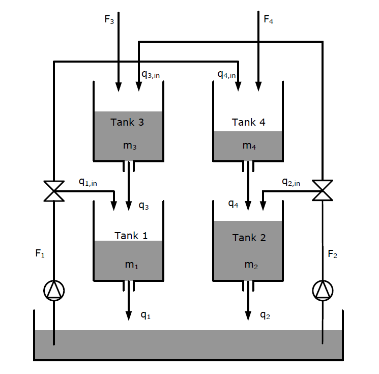
Fig. 1 illustrates the modified four-tank system (MFTS). The mass balances are modelled as ODEs as presented by [22]. However, we model the stochastic disturbances explicitly as states. The disturbances follow the SDEs


$\displaystyle d\boldsymbol{F}_{3}(t)$	$\displaystyle=\lambda_{1}\left(\bar{F}_{3}(t)-\boldsymbol{F}_{3}(t)\right)dt+\sigma_{1}d\boldsymbol{\omega}_{1}(t),$	(50a)
$\displaystyle d\boldsymbol{F}_{4}(t)$	$\displaystyle=\lambda_{2}\left(\bar{F}_{4}(t)-\boldsymbol{F}_{4}(t)\right)dt+\sigma_{2}d\boldsymbol{\omega}_{2}(t).$	(50b)

The resulting system is described by a continuous-discrete nonlinear system as described in (1).The performance of each state estimation method is evaluated in terms of the mean absolute percentage error (MAPE) , such that

\displaystyle MAPE

\displaystyle=\frac{1}{nN}\sum_{k=1}^{N}\sum_{i=1}^{n}\left|\frac{x_{i,k}-\hat{x}_{i,k}}{x_{i,k}}\right|,

(51)

where $N$ is the number of observations and $n$ is the dimension of the state. The MAPE is computed separately for the states representing the liquid mass and the state representing the disturbances, as MAPE_x and MAPE_d respectively.

IV-A Simulation example

Fig. 2 illustrates the simulation example and Table I describes the results. We simulation is $30$ minutes, with $120$ equidistant samples. The simulation and estimation are computed with internal step sizes of $1000$ and $100$ respectively. The UKF has the parameter set $\left[\beta,\alpha,\kappa\right]=\left[2.0,0.001,0.0\right]$ . The EnKF and PF has sampling sizes of $250$ and $1000$ respectively. The disturbances are modelled with $\lambda_{1}=\lambda_{2}=0.1$ and $\sigma_{1}=\sigma_{2}=5.0$ for the simulation. For the EKF, EnKF, and PF, $\sigma_{1}=\sigma_{2}=5.0$ and for the UKF $\sigma_{1}=\sigma_{2}=1.0$ . $\lambda_{1}=\lambda_{2}=0.0$ for the EKF and UKF and $\lambda_{1}=\lambda_{2}=$ 2.0e-3 for the EnKF and PF.

From the results presented in Fig. 2 and Table I, we see many of the properties described in the discussion of Section III. The EKF and UKF are demonstrated the be the most computationally efficient methods, where EKF seem to be outperforming UKF in this particular numerical experiment. Furthermore, the EnKF and PF show better accuracy both in estimating state and disturbance variables, but at the cost of lower computational efficiency.

TABLE I: run-times for time update (TU) and measurement update (MU), and MAPE for states (MAPE_x) and disturbances (MAPE_d).

name	EKF	UKF	EnKF	PF
time TU [s]	3.09e-01	2.90e+00	3.38e+01	1.36e+02
time MU [s]	1.22e-02	4.14e-02	2.30e-01	1.05e+00
MAPE_x [%]	2.55e+00	2.97e+00	2.35e+00	2.40e+00
MAPE_d [%]	1.57e+01	1.75e+01	1.47e+01	1.37e+01

Fig. 2: State estimation for simulation of the modified four-tank system. For the simulation model

\bar{F}_{i}\in\{100,200,300\}

for

i\in\{3,4\}

. The nominal values are kept constant at

150

for the state estimators.

V Conclusion

In conclusion, we have presented four methods for state estimation in continuous-discrete nonlinear systems involving stochastic differential equations: the EKF, UKF, EnKF, and a PF. In Matlab, the state estimation methods have been implemented for non-stiff systems and a numerical experiment has been performed on a simulated MFTS. The performance of each state estimation method has been evaluated in terms of run-times for time and measurement updates and the accuracy have been evaluated in terms of the MAPE for the state and disturbance estimates.

References

[1] R. E. Kalman, “A new approach to linear filtering and prediction problems,” Journal of Basic Engineering, vol. 82, no. 1, pp. 35–45, 1960.
[2] A. H. Jazwinski, Stochastic processes and filtering theory. Dover Publication, Inc., 2007.
[3] J. B. Rawlings, D. Q. Mayne, and M. Diehl, Model predictive control: theory, computation, and design, 2nd ed. Nob Hill Publishing Madison, WI, 2017.
[4] P. Frogerais, J.-J. Bellanger, and L. Senhadji, “Various ways to compute the continuous-discrete extended Kalman filter,” IEEE Transactions on Automatic Control, vol. 57, no. 4, pp. 1000–1004, 2011.
[5] E. L. Haseltine and J. B. Rawlings, “Critical evaluation of extended Kalman filtering and moving-horizon estimation,” Industrial & Engineering Chemistry Research, vol. 44, no. 8, pp. 2451–2460, 2005.
[6] R. S. Bucy and P. D. Joseph, Filtering for stochastic processes with applications to guidance. American Mathematical Society, 2005.
[7] J. B. Jørgensen, H. Madsen, P. G. Thomsen, and M. R. Kristensen, “A computationally efficient and robust implementation of the continuous-discrete extended Kalman filter,” in proceedings of the 2007 Americal Control Conference (ACC), New York, NY, USA. July 11-13, 2007, pp. 3706–3712.
[8] S. J. Julier and J. K. Uhlmann, “Unscented filtering and nonlinear estimation,” Proceedings of the IEEE, vol. 92, no. 3, pp. 401–422, 2004.
[9] E. A. Wan and R. van der Merwe, “The unscented Kalman filter for nonlinear estimation,” in proceedings of the IEEE 2000 Adaptive Systems for Signal Processing, Communications, and Control Symposium (AS-SPCC), Lake Louise, A.B., Canada. October 4, 2000, pp. 153–158.
[10] R. Kandepu, B. Foss, and L. Imsland, “Applying the unscented Kalman filter for nonlinear state estimation,” Journal of Process Control, vol. 18, no. 7-8, pp. 753–768, 2008.
[11] F. De Vivo, A. Brandl, M. Battipede, and P. Gili, “Joseph covariance formula adaptation to square-root sigma-point Kalman filters,” Nonlinear Dynamics, vol. 88, no. 3, pp. 1969–1986, 2017.
[12] R. Zanetti and K. J. DeMars, “Joseph formulation of unscented and quadrature filters with application to consider states,” Journal of Guidance, Control, and Dynamics, vol. 36, no. 6, pp. 1860–1864, 2013.
[13] R. van der Merwe, A. Doucet, N. De Freitas, and E. A. Wan, “The unscented particle filter,” in proceedings of the 13th Advances in Neural Information Processing Systems (NIPS), Vancouver, B.C., Canada. December 3-8, 2001, pp. 584–590.
[14] S. Gillijns, O. B. Mendoza, J. Chandrasekar, B. L. R. De Moor, D. S. Bernstein, and A. Ridley, “What is the ensemble Kalman filter and how well does it work?” in proceedings of the 2006 American Control Conference (ACC), Minneapolis, M.N., USA. June 14-16, 2006, pp. 4448–4453.
[15] I. Myrseth and H. Omre, “Hierarchical ensemble Kalman filter,” SPE Journal, vol. 15, no. 2, pp. 569–580, 2010.
[16] M. Roth, C. Fritsche, G. Hendeby, and F. Gustafison, “The ensemble Kalman filter and its relations to other nonlinear filters,” in proceedings of the 23rd European Signal Processing Conference (EUSIPCO), Nice, France. August 31-September 4, 2015, pp. 1236–1240.
[17] M. S. Arulampalam, S. Maskell, N. Gordon, and T. Clapp, “A tutorial on particle filters for online nonlinear/non-gaussian bayesian tracking,” IEEE Transactions on Signal Processing, vol. 50, no. 2, pp. 174–188, 2002.
[18] J. B. Rawlings and B. R. Bakshi, “Particle filtering and moving horizon estimation,” Computers & Chemical Engineering, vol. 30, no. 10-12, pp. 1529–1541, 2006.
[19] A. V. Shenoy, J. Prakash, K. B. McAuley, V. Prasad, and S. L. Shah, “Practical issues in the application of the particle filter for estimation of chemical processes,” in proceedings of the 18th IFAC World Congress, Italy, Milano. August 28-September 2, 2011, pp. 2773–2778.
[20] A. Tulsyan, R. B. Gopaluni, and S. R. Khare, “Particle filtering without tears: a primer for beginners,” Computers & Chemical Engineering, vol. 95, pp. 130–145, 2016.
[21] J. B. Jørgensen, M. R. Kristensen, P. G. Thomsen, and H. Madsen, New extended Kalman filter algorithms for stochastic differential algebraic equations. Springer Berlin Heidelberg, 2007, pp. 359–366.
[22] S. N. M. Azam and J. B. Jørgensen, “Modeling and simulation of a modified quadruple tank system,” in proceedings of the 2015 IEEE International Conference on Control System, Computing and Engineering (ICCSCE), Penang, Malaysia. November 27-29, 2015, pp. 365–370.


$\displaystyle\hat{x}_{k\|k}$	$\displaystyle=\hat{x}_{k\|k-1}+K_{f_{x},k}e_{k},$	(9a)
$\displaystyle P_{k\|k}$	$\displaystyle=P_{k\|k-1}-K_{f_{x},k}R_{e,k}K_{f_{x},k}^{T}$	(9b)
$\displaystyle\begin{split}&=\left(I-K_{f_{x},k}C_{k}\right)P_{k\|k-1}\left(I-K_{f_{x},k}C_{k}\right)^{T}\\ &+K_{f_{x},k}RK_{f_{x},k}^{T},\end{split}$		(9c)


$\displaystyle\hat{x}_{k+1\|k}$	$\displaystyle=\sum_{i=0}^{2\bar{n}}\bar{W}_{m}^{(i)}\hat{x}_{k+1\|k}^{(i)},$	(19a)
$\displaystyle P_{k+1\|k}$	$\displaystyle=\sum_{i=0}^{2\bar{n}}\bar{W}_{c}^{(i)}\left(\hat{x}_{k+1\|k}^{(i)}-\hat{x}_{k+1\|k}\right)\left(\hat{x}_{k+1\|k}^{(i)}-\hat{x}_{k+1\|k}\right)^{T}.$	(19b)


$\displaystyle\hat{x}_{k\|k-1}^{(0)}$	$\displaystyle=\hat{x}_{k\|k-1},$	(22a)
$\displaystyle\hat{x}_{k\|k-1}^{(i)}$	$\displaystyle=\hat{x}_{k\|k-1}+\sqrt{c}\left(\sqrt{P_{k\|k-1}}\right)_{i},$	(22b)
$\displaystyle\hat{x}_{k\|k-1}^{(n_{x}+i)}$	$\displaystyle=\hat{x}_{k\|k-1}-\sqrt{c}\left(\sqrt{P_{k\|k-1}}\right)_{i},$	(22c)


$\displaystyle R_{zz,k\|k-1}$	$\displaystyle=\sum_{i=0}^{2n_{x}}W_{c}^{(i)}\left(\hat{z}_{k\|k-1}^{(i)}-\hat{z}_{k\|k-1}\right)\left(\hat{z}_{k\|k-1}^{(i)}-\hat{z}_{k\|k-1}\right)^{T},$	(25a)
$\displaystyle R_{e,k}$	$\displaystyle=R_{yy,k\|k-1}=R_{zz,k\|k-1}+R,$	(25b)
$\displaystyle R_{xy,k\|k-1}$	$\displaystyle=\sum_{i=0}^{2n_{x}}W_{c}^{(i)}\left(\hat{x}_{k\|k-1}^{(i)}-\hat{x}_{k\|k-1}\right)\left(\hat{z}_{k\|k-1}^{(i)}-\hat{z}_{k\|k-1}\right)^{T}.$	(25c)


$\displaystyle\hat{x}_{k\|k}$	$\displaystyle=\hat{x}_{k\|k-1}+K_{f_{x},k}e_{k},$	(27a)
$\displaystyle P_{k\|k}$	$\displaystyle=P_{k\|k-1}-K_{f_{x},k}R_{e,k}K_{f_{x},k}^{T}.$	(27b)

State Estimation Methods for Continuous-Discrete Nonlinear Systems involving Stochastic Differential Equations

Abstract

I Introduction

II Nonlinear Continuous-Discrete Stochastic Differential Equation Models

III State Estimation in Nonlinear Systems

III-A Continuous-discrete extended Kalman filter

III-A1 Time update

III-A2 Measurement update

III-B Continuous-discrete unscented Kalman filter

III-B1 Time update

III-B2 Measurement update

III-C Continuous-discrete ensemble Kalman filter

III-C1 Time update

III-C2 Measurement update

III-D Continous-discrete particle filter

III-D1 Time update

III-D2 Measurement update

III-E Discussion of methods

IV Example – Modified Four-Tank System

IV-A Simulation example

V Conclusion

References

State Estimation Methods
for Continuous-Discrete Nonlinear Systems
involving Stochastic Differential Equations