跳到论文正文
W Papers独立论文阅读器 arXiv:2205.02585 论文正文 计算阅读时间 · 0%
引用这篇论文根据当前论文元数据生成,正式投稿前建议核对。


License: arXiv.org perpetual non-exclusive license
arXiv:2205.02585v2 [math.CV] 27 Nov 2022

Trigonometric Convexity for the Multidimensional Indicator after Ivanov

Aleksandr Mkrtchyan1,2 1. Siberian Federal University, Russia
2. Institute of Mathematics NAS, Armenia

Armen Vagharshakyan3,4 3. Institute of Mathematics NAS, Armenia
4. Regional Mathematical Center of the
Southern Federal University, Russia
Abstract

Multidimensional indicator after Ivanov is a generalization of the notion of indicator, that is well-known for analytic functions in one complex variable, to analytic functions in several complex variables. We prove an analogue of trigonometric convexity for it. Additionally, we show that our estimate is sharp. The proof is based on the multidimensional analogue of the sectorial Fourier inversion formula.
Keywords: analytic functions in several complex variables, indicator function, analytic continuation
MSC classification: 32A26, 42B10, 32C30

1 Introduction.

1.1 Main results.

We review the notion of indicator for analytic functions in one complex variable (see section 1.2) and its multidimensional analogues for functions in several complex variables (see section 1.3); in particular, we treat the notion of multidimensional indicator after Ivanov.

As explained in remark 1.3.1, our main theorem 1.1.5 establishes an analogue of trigonometric convexity for the multidimensional indicator after Ivanov. We preface formulation of theorem 1.1.5 by the following definitions:

Definition 1.1.1.

Denote by Δαj⊂ℂ\Delta_{\alpha_{j}}\subset\mathbb{C} the open sector determined by the angle 0<αj<π/20<\alpha_{j}<\pi/2 as follows:

Δαj={zj∈ℂ∖{0}:|arg⁡(zj)|<αj}.\Delta_{\alpha_{j}}=\{z_{j}\in\mathbb{C}\setminus\{0\}\colon\left|\arg\left(z_{j}\right)\right|<\alpha_{j}\}.
Definition 1.1.2.

Recall that a function ff is of finite exponential type (h1,…,hn)\left(h_{1},\dots,h_{n}\right) in Δα1×⋯×Δαn\Delta_{\alpha_{1}}\times\dots\times\Delta_{\alpha_{n}} if for any ε>0\varepsilon>0 there exists a constant kε≥0k_{\varepsilon}\geq 0 such that

|f⁡(z1,…,zn)|≤kε​e(h1+ε)​|z1|+⋯+(hn+ε)​|zn|, for all ​zj∈Δj, 1≤j≤n.\left|f\left(z_{1},\dots,z_{n}\right)\right|\leq k_{\varepsilon}e^{(h_{1}+\varepsilon)\left|z_{1}\right|+\dots+\left(h_{n}+\varepsilon\right)\left|z_{n}\right|},\quad\text{ for all }z_{j}\in\Delta_{j},\;1\leq j\leq n. (1.1.1)

Note that in this article we tacitly assume that h1,…,hn≥0h_{1},\dots,h_{n}\geq 0.

Definition 1.1.3.

Denote by E​x​p​(α1,…,αn)Exp\left(\alpha_{1},\dots,\alpha_{n}\right) the class of functions ff that are analytic and are of finite exponential type in Δ1×⋯×Δn.\Delta_{1}\times\dots\times\Delta_{n}.

Definition 1.1.4.

Following Ivanov [1], for f∈E​x​p​(α1,…,αn)f\in Exp\left(\alpha_{1},\dots,\alpha_{n}\right) denote by Tf​(θ→)T_{f}\left(\vec{\theta}\right) the following:

Tf(θ→)={\displaystyle T_{f}\left(\vec{\theta}\right)=\{ ν→∈ℝn:ln⁡|f⁡(r→​ei​θ→)|≤ν1​r1+…+νn​rn+Cν→,θ→,\displaystyle\vec{\nu}\in\mathbb{R}^{n}:\ln{\left|f\left(\vec{r}e^{i\vec{\theta}}\right)\right|}\leq\nu_{1}r_{1}+...+\nu_{n}r_{n}+C_{\vec{\nu},\vec{\theta}}, (1.1.2)
for some Cν→,θ→, for all r→∈ℝ+n},\displaystyle\text{ for some }C_{\vec{\nu},\vec{\theta}},\text{ for all }\vec{r}\in\mathbb{R}^{n}_{+}\},

here r→​ei​θ→\vec{r}e^{i\vec{\theta}} denotes the vector (r1​ei​θ1,…,rn​ei​θn).\left(r_{1}e^{i\theta_{1}},...,r_{n}e^{i\theta_{n}}\right).

Theorem 1.1.5.

Let a function f∈E​x​p​(α1,α2)f\in Exp\left(\alpha_{1},\alpha_{2}\right) and the numbers A1+,A2+,A1−,A2−A^{+}_{1},A^{+}_{2},A^{-}_{1},A^{-}_{2} satisfy:

(A1+,A2+)∈T¯f​(α1,α2),(A1−,A2−)∈T¯f​(−α1,−α2),\displaystyle\left(A^{+}_{1},A^{+}_{2}\right)\in\overline{T}_{f}\left(\alpha_{1},\alpha_{2}\right),\quad\left(A^{-}_{1},A^{-}_{2}\right)\in\overline{T}_{f}\left(-\alpha_{1},-\alpha_{2}\right),
(A1+,A2−)∈T¯f​(α1,−α2),(A1−,A2+)∈T¯f​(−α1,α2).\displaystyle\left(A^{+}_{1},A^{-}_{2}\right)\in\overline{T}_{f}\left(\alpha_{1},-\alpha_{2}\right),\quad\left(A^{-}_{1},A^{+}_{2}\right)\in\overline{T}_{f}\left(-\alpha_{1},\alpha_{2}\right).

Then we have

(C1,C2)∈T¯f​(θ1,θ2),\left(C_{1},C_{2}\right)\in\overline{T}_{f}\left(\theta_{1},\theta_{2}\right),

where the constants C1,C2C_{1},C_{2} are determined by the following formulas:

C1​sin⁡(2​α1)=A1+​sin⁡(θ1+α1)+A1−​sin⁡(α1−θ1),\displaystyle C_{1}\sin\left(2\alpha_{1}\right)=A^{+}_{1}\sin\left(\theta_{1}+\alpha_{1}\right)+A^{-}_{1}\sin\left(\alpha_{1}-\theta_{1}\right), (1.1.3)
C2​sin⁡(2​α2)=A2+​sin⁡(θ2+α2)+A2−​sin⁡(α2−θ2).\displaystyle C_{2}\sin\left(2\alpha_{2}\right)=A^{+}_{2}\sin\left(\theta_{2}+\alpha_{2}\right)+A^{-}_{2}\sin\left(\alpha_{2}-\theta_{2}\right). (1.1.4)

Theorem 1.1.5 can be paraphrased as follows:

Remark 1.1.6.

Let a function f∈E​x​p​(α1,α2)f\in Exp\left(\alpha_{1},\alpha_{2}\right) and the numbers A1+,A2+,A1−,A2−A^{+}_{1},A^{+}_{2},A^{-}_{1},A^{-}_{2} satisfy:

|f⁡(z1,z2)|≤kε​e(A1++ε)​|z1|+(A2++ε)​|z2|,for ​arg⁡(z1)=α1,arg⁡(z2)=α2,\displaystyle\left|f\left(z_{1},z_{2}\right)\right|\leq k_{\varepsilon}e^{(A^{+}_{1}+\varepsilon)\left|z_{1}\right|+\left(A^{+}_{2}+\varepsilon\right)\left|z_{2}\right|},\quad\text{for }\arg(z_{1})=\alpha_{1},\;\arg\left(z_{2}\right)=\alpha_{2},
|f⁡(z1,z2)|≤kε​e(A1++ε)​|z1|+(A2−+ε)​|z2|,for ​arg⁡(z1)=α1,arg⁡(z2)=−α2,\displaystyle\left|f\left(z_{1},z_{2}\right)\right|\leq k_{\varepsilon}e^{(A^{+}_{1}+\varepsilon)\left|z_{1}\right|+\left(A^{-}_{2}+\varepsilon\right)\left|z_{2}\right|},\quad\text{for }\arg(z_{1})=\alpha_{1},\;\arg\left(z_{2}\right)=-\alpha_{2},
|f⁡(z1,z2)|≤kε​e(A1−+ε)​|z1|+(A2++ε)​|z2|,for ​arg⁡(z1)=−α1,arg⁡(z2)=α2,\displaystyle\left|f\left(z_{1},z_{2}\right)\right|\leq k_{\varepsilon}e^{(A^{-}_{1}+\varepsilon)\left|z_{1}\right|+\left(A^{+}_{2}+\varepsilon\right)\left|z_{2}\right|},\quad\text{for }\arg(z_{1})=-\alpha_{1},\;\arg\left(z_{2}\right)=\alpha_{2},
|f⁡(z1,z2)|≤kε​e(A1−+ε)​|z1|+(A2−+ε)​|z2|,for ​arg⁡(z1)=−α1,arg⁡(z2)=−α2,\displaystyle\left|f\left(z_{1},z_{2}\right)\right|\leq k_{\varepsilon}e^{(A^{-}_{1}+\varepsilon)\left|z_{1}\right|+\left(A^{-}_{2}+\varepsilon\right)\left|z_{2}\right|},\quad\text{for }\arg(z_{1})=-\alpha_{1},\;\arg\left(z_{2}\right)=-\alpha_{2}, (1.1.5)

where by the value of the function ff on the mentioned rays we mean ff’s non-tangential limit (see [2], remark 2.1 for details). Then for any ε>0\varepsilon>0 there exists a constant kε′>0k^{\prime}_{\varepsilon}>0 such that

|f⁡(z1,z2)|≤kε′​e(C1+ε)​|z1|+(C2+ε)​|z2|,for ​arg⁡(z1)=θ1,arg⁡(z2)=θ2,\left|f\left(z_{1},z_{2}\right)\right|\leq k^{\prime}_{\varepsilon}e^{(C_{1}+\varepsilon)\left|z_{1}\right|+\left(C_{2}+\varepsilon\right)\left|z_{2}\right|},\quad\text{for }\arg\left(z_{1}\right)=\theta_{1},\;\arg\left(z_{2}\right)=\theta_{2}, (1.1.6)

where the constants C1,C2C_{1},C_{2} are determined by the following formulas:

C1​sin⁡(2​α1)=A1+​sin⁡(θ1+α1)+A1−​sin⁡(α1−θ1),\displaystyle C_{1}\sin\left(2\alpha_{1}\right)=A^{+}_{1}\sin\left(\theta_{1}+\alpha_{1}\right)+A^{-}_{1}\sin\left(\alpha_{1}-\theta_{1}\right),
C2​sin⁡(2​α2)=A2+​sin⁡(θ2+α2)+A2−​sin⁡(α2−θ2).\displaystyle C_{2}\sin\left(2\alpha_{2}\right)=A^{+}_{2}\sin\left(\theta_{2}+\alpha_{2}\right)+A^{-}_{2}\sin\left(\alpha_{2}-\theta_{2}\right).

In section 3 we derive theorem 1.1.5 from theorem 1.1.9 that serves as a two-dimensional analogue of the Fourier inversion formula (see [2], theorem 1.2 and [3]) for functions of exponential type in a sector. We preface formulation of theorem 1.1.9 by the following definitions:

Definition 1.1.7.

Let f∈E​x​p​(α1,α2)f\in Exp\left(\alpha_{1},\alpha_{2}\right) and let the numbers A1+,A2+,A1−,A2−A^{+}_{1},A^{+}_{2},A^{-}_{1},A^{-}_{2} satisfy 1.1.5. Define the function mm as ff’s two-dimensional concatenated Laplace transform. Namely, the domain of function mm is the Cartesian product Ω1×Ω2,\Omega_{1}\times\Omega_{2}, where

Ω1=Ω1+∪Ω1−,\displaystyle\Omega_{1}=\Omega_{1}^{+}\cup\Omega_{1}^{-},
Ω2=Ω2+∪Ω2−,\displaystyle\Omega_{2}=\Omega_{2}^{+}\cup\Omega_{2}^{-},

and in turn

Ω1+={ω1:R​e​(ω1​ei​α1)<−A1+},\displaystyle\Omega_{1}^{+}=\left\{\omega_{1}\colon Re\left(\omega_{1}e^{i\alpha_{1}}\right)<-A^{+}_{1}\right\}, (1.1.7)
Ω1−={ω1:R​e​(ω1​e−i​α1)<−A1−},\displaystyle\Omega_{1}^{-}=\left\{\omega_{1}\colon Re\left(\omega_{1}e^{-i\alpha_{1}}\right)<-A^{-}_{1}\right\},
Ω2+={ω2:R​e​(ω2​ei​α2)<−A2+},\displaystyle\Omega_{2}^{+}=\left\{\omega_{2}\colon Re\left(\omega_{2}e^{i\alpha_{2}}\right)<-A^{+}_{2}\right\},
Ω2−={ω2:R​e​(ω2​e−i​α2)<−A2−},\displaystyle\Omega_{2}^{-}=\left\{\omega_{2}\colon Re\left(\omega_{2}e^{-i\alpha_{2}}\right)<-A^{-}_{2}\right\},
Refer to caption
Figure 1: The set Ω\Omega

(see figure 1 on page 1). The function mm is defined on Ω1×Ω2\Omega_{1}\times\Omega_{2} by the following four formulas:

m(ω1,ω2)=−14​π2∫ei​α2[0,+∞)∫ei​α1[0,+∞)f(ζ1,ζ2)eω1​ζ1+ω2​ζ2dζ1dζ2,\displaystyle m\left(\omega_{1},\omega_{2}\right)=\frac{-1}{4\pi^{2}}\int_{e^{i\alpha_{2}}[0,+\infty)}\int_{e^{i\alpha_{1}}[0,+\infty)}f\left(\zeta_{1},\zeta_{2}\right)e^{\omega_{1}\zeta_{1}+\omega_{2}\zeta_{2}}d\zeta_{1}d\zeta_{2}, (1.1.8)
for ​ω1∈Ω1+,ω2∈Ω2+,\displaystyle\quad\quad\quad\quad\text{for }\omega_{1}\in\Omega_{1}^{+},\;\omega_{2}\in\Omega_{2}^{+},
m(ω1,ω2)=−14​π2∫ei​α2[0,+∞)∫e−i​α1[0,+∞)f(ζ1,ζ2)eω1​ζ1+ω2​ζ2dζ1dζ2,\displaystyle m\left(\omega_{1},\omega_{2}\right)=\frac{-1}{4\pi^{2}}\int_{e^{i\alpha_{2}}[0,+\infty)}\int_{e^{-i\alpha_{1}}[0,+\infty)}f\left(\zeta_{1},\zeta_{2}\right)e^{\omega_{1}\zeta_{1}+\omega_{2}\zeta_{2}}d\zeta_{1}d\zeta_{2},
for ​ω1∈Ω1+,ω2∈Ω2−,\displaystyle\quad\quad\quad\quad\text{for }\omega_{1}\in\Omega_{1}^{+},\;\omega_{2}\in\Omega_{2}^{-},
m(ω1,ω2)=−14​π2∫e−i​α2[0,+∞)∫ei​α1[0,+∞)f(ζ1,ζ2)eω1​ζ1+ω2​ζ2dζ1dζ2,\displaystyle m\left(\omega_{1},\omega_{2}\right)=\frac{-1}{4\pi^{2}}\int_{e^{-i\alpha_{2}}[0,+\infty)}\int_{e^{i\alpha_{1}}[0,+\infty)}f\left(\zeta_{1},\zeta_{2}\right)e^{\omega_{1}\zeta_{1}+\omega_{2}\zeta_{2}}d\zeta_{1}d\zeta_{2},
for ​ω1∈Ω1−,ω2∈Ω2+,\displaystyle\quad\quad\quad\quad\text{for }\omega_{1}\in\Omega_{1}^{-},\;\omega_{2}\in\Omega_{2}^{+},
m(ω1,ω2)=−14​π2∫e−i​α2[0,+∞)∫e−i​α1[0,+∞)f(ζ1,ζ2)eω1​ζ1+ω2​ζ2dζ1dζ2,\displaystyle m\left(\omega_{1},\omega_{2}\right)=\frac{-1}{4\pi^{2}}\int_{e^{-i\alpha_{2}}[0,+\infty)}\int_{e^{-i\alpha_{1}}[0,+\infty)}f\left(\zeta_{1},\zeta_{2}\right)e^{\omega_{1}\zeta_{1}+\omega_{2}\zeta_{2}}d\zeta_{1}d\zeta_{2},
for ​ω1∈Ω1−,ω2∈Ω2−.\displaystyle\quad\quad\quad\quad\text{for }\omega_{1}\in\Omega_{1}^{-},\;\omega_{2}\in\Omega_{2}^{-}.
Definition 1.1.8.

For a class of functions E​x​p​(α1,α2),Exp\left(\alpha_{1},\alpha_{2}\right), denote by Γ1\Gamma_{1} and Γ2\Gamma_{2} the curves given by the following parametrizations:

γ1:ℝ→ℂ,\displaystyle\gamma_{1}\colon\mathbb{R}\rightarrow\mathbb{C},
γ1(t)=p1−iei​α1|t|,for t∈(−∞,0],\displaystyle\gamma_{1}(t)=p_{1}-ie^{i\alpha_{1}}|t|,\quad\text{for }t\in(-\infty,0],
γ1(t)=p1+ie−i​α1|t|,for t∈(0,+∞],\displaystyle\gamma_{1}(t)=p_{1}+ie^{-i\alpha_{1}}|t|,\quad\text{for }t\in(0,+\infty], (1.1.9)

(see figure 2 on page 2), and the real number p1p_{1} appearing in parametrization (1.1.8), is chosen in such a way that it satisfies inequality

p1​cos⁡(α1)<−h1p_{1}\cos(\alpha_{1})<-h_{1} (1.1.10)
Refer to caption
Figure 2: The curve Γ1\Gamma_{1}

and correspondingly the curve Γ2\Gamma_{2} is parameterized by

γ2:ℝ→ℂ,\displaystyle\gamma_{2}\colon\mathbb{R}\rightarrow\mathbb{C},
γ2(t)=p2−iei​α2|t|,for t∈(−∞,0],\displaystyle\gamma_{2}(t)=p_{2}-ie^{i\alpha_{2}}|t|,\quad\text{for }t\in(-\infty,0],
γ2(t)=p2+ie−i​α2|t|,for t∈(0,+∞],\displaystyle\gamma_{2}(t)=p_{2}+ie^{-i\alpha_{2}}|t|,\quad\text{for }t\in(0,+\infty], (1.1.11)

and the real number p2p_{2} appearing in parametrization (1.1.8), is chosen in such a way that it satisfies inequality

p2​cos⁡(α2)<−h2,p_{2}\cos(\alpha_{2})<-h_{2}, (1.1.12)
Theorem 1.1.9.

For a function f∈E​x​p​(α1,α2)f\in Exp\left(\alpha_{1},\alpha_{2}\right) the following Fourier inversion formula holds:

f⁡(z1,z2)=∫Γ1∫Γ2m⁡(ω1,ω2)​e−ω1​z1−ω2​z2​d​ω2​𝑑ω,for ​z1∈Δ1,z2∈Δ2.f\left(z_{1},z_{2}\right)=\int_{\Gamma_{1}}\int_{\Gamma_{2}}m\left(\omega_{1},\omega_{2}\right)e^{-\omega_{1}z_{1}-\omega_{2}z_{2}}d\omega_{2}d\omega,\quad\text{for }z_{1}\in\Delta_{1},\;z_{2}\in\Delta_{2}. (1.1.13)

Theorem 1.1.9 is proved in section 2.

We complement theorem 1.1.5 by the following remarks:

Remark 1.1.10.

Theorem 1.1.5 is stated for functions of two complex variables. The corresponding theorem for functions of nn complex variables also holds.

Remark 1.1.11.

Theorem 1.1.5 is sharp: that is, there exists a function ff for whom: the assumptions of theorem 1.1.5 are satisfied, and the inequality (1.1.6) is an equality.

Remark 1.1.11 is proved in section 4.

Remark 1.1.12.

Integral representation (1.1.13) in 1.1.9 could be compared to multivariate integrals of Mellin-Barnes type [4],[5].

1.2 Indicators of functions in one complex variable.

We say that an entire function f:ℂ→ℂf\colon\mathbb{C}\rightarrow\mathbb{C} is of exponential type if

lim supz→∞ln+⁡|f⁡(z)||z|<+∞.\limsup_{z\to\infty}\frac{\ln^{+}|f(z)|}{|z|}<+\infty. (1.2.1)

The notion of indicator of an entire function of exponential type was introduced by Phragmen and Lindeleph [6],[7] as follows:

hf​(α):=lim supr→∞ln⁡|f⁡(r​ei​α)|r,α∈ℝ.h_{f}(\alpha):=\limsup_{r\to\infty}\frac{\ln\left|f\left(re^{i\alpha}\right)\right|}{r},\;\;\alpha\in\mathbb{R}. (1.2.2)

The indicator hf​(α)h_{f}(\alpha) describes the growth of function ff along the ray ei​α[0,+∞).e^{i\alpha}[0,+\infty). It follows from definition (1.2.2) that the indicator hf​(α)h_{f}(\alpha) is a real-valued 2​π2\pi-periodic function. It also follows that the indicator of the product of two functions does not exceed the sum of the indicators of the factors,

hf​g​(α)≤hf​(α)+hg​(α),h_{fg}(\alpha)\leq h_{f}(\alpha)+h_{g}(\alpha),

and that the indicator of the sum of two functions does not exceed the larger of the two indicators,

hf+g​(α)≤max⁡(hf​(α),hg​(α)).h_{f+g}(\alpha)\leq\max\left(h_{f}(\alpha),h_{g}(\alpha)\right).

One of the main properties of the indicator hθ​(α)h_{\theta}(\alpha) is its trigonometric convexity [8],[9]: if α1<α<α2\alpha_{1}<\alpha<\alpha_{2} and α2−α1<π,\alpha_{2}-\alpha_{1}<\pi, then the following inequality holds:

hf​(α)​sin⁡(α2−α1)≤hf​(α1)​sin⁡(α2−α)+hf​(α2)​sin⁡(α−α1).h_{f}(\alpha)\sin{(\alpha_{2}-\alpha_{1})}\leq h_{f}(\alpha_{1})\sin{(\alpha_{2}-\alpha)}+h_{f}(\alpha_{2})\sin{(\alpha-\alpha_{1})}. (1.2.3)

The following property follows from the trigonometric convexity (1.2.3) [8]: if the indicator is bounded on an open interval, then it is continuous. The latter claim does not hold for a closed interval.

The notion of indicator is known to be an important tool in some methods regarding to finding analytic continuation [10], [11],[12],[13]. In particular, the indicator appears in problems relating to analytic continuation of power series via interpolation of coefficients. It also plays a role in problems relating to localization of singularities of power series [14].

Let

f⁡(z)=∑k=0∞akk!​zk,f(z)=\sum_{k=0}^{\infty}{\frac{a_{k}}{k!}z^{k}},

be the power-series representation of the entire function f.f. Consider its Borel transform defined by the Laurent series in the following way:

g⁡(ω)=∑k=0∞ak​ω−k−1.g(\omega)=\sum_{k=0}^{\infty}{a_{k}\omega^{-k-1}}. (1.2.4)

The interrelation between the set of singularities of gg and the indicator of ff is described by Polya’s theorem [15], [16]:

Theorem 1.2.1 (Polya).

Let ff be an entire function of exponential type. Denote by K⊂ℂK\subset\mathbb{C} the convex set whose support function

k⁡(θ)=supω∈KR​e​(ω​e−i​θ)k(\theta)=\sup_{\omega\in K}Re\left(\omega e^{-i\theta}\right)

is determined by ff’s indicator as follows:

k⁡(−θ)=hf​(θ).k(-\theta)=h_{f}(\theta). (1.2.5)

Then ff can be restored by

f⁡(z)=12​π​i​∫Γg⁡(ω)​ez​ω​𝑑ω,f(z)=\frac{1}{2\pi i}\int_{\Gamma}g(\omega)e^{z\omega}d\omega, (1.2.6)

where Γ\Gamma is a closed contour containing the set K,K, and gg (1.2.4) is the Borel transform of f.f. Additionally, KK is the smallest convex set such that gg is analytic in ℂ∖K.\mathbb{C}\setminus K.

1.3 Indicators of functions in several complex variables.

The works of Ronkin [16], Lelon [17], Levin [8], Ivanov [1], Kiselman [18] and others are dedicated to exploring multidimensional analogues of the indicator function. We say that f⁡(z→)=f⁡(z1,…,zn)f\left(\vec{z}\right)=f(z_{1},...,z_{n}) is an nn-valued entire function of exponential type if ff is holomorphic in ℂn,\mathbb{C}^{n},

f⁡(z→)∈𝒪⁡(ℂn),f\left(\vec{z}\right)\in\mathcal{O}(\mathbb{C}^{n}),

and if there exist constants k,σ1,…,σnk,\sigma_{1},...,\sigma_{n} such that

|f⁡(z→)|≤k​eσ1​|z1|+…+σn​|zn|,for ​z→∈ℂn.\left|f\left(\vec{z}\right)\right|\leq ke^{\sigma_{1}|z_{1}|+...+\sigma_{n}|z_{n}|},\quad\text{for }\vec{z}\in\mathbb{C}^{n}. (1.3.1)

In the case of several complex variables, different characteristics of an analytic function’s growth in directions have been introduced. For example, introduce the radial indicator of the function ff as follows [16], [17]:

Lr​(z,f)=lim supt→∞ln⁡|f⁡(t​z)|t,z∈ℂnL_{r}(z,f)=\limsup_{t\to\infty}\frac{\ln|f(tz)|}{t},\;\;z\in\mathbb{C}^{n}

and correspondingly introduce regularization of the function L⁡(z,f)L(z,f) as follows:

L∗​(z,f)=lim supz′→zL⁡(z,f)L^{\ast}(z,f)=\limsup_{z^{\prime}\to z}L(z,f) (1.3.2)

We will refer to L∗​(z,f)L^{\ast}(z,f) as regularized radial indicator of the function ff. Just as in the on-dimensional case the function L∗​(z,f)L^{\ast}(z,f) is semi-continuous from above. Note that the regularized radial indicator is a plurisubharmonic function in ℂn.\mathbb{C}^{n}. Consequently, more information about its properties may be found in works related to plurisubharmonic functions in potential theory [18] and their different generalizations [19], [20].

Another charateristic of an analytic functions growth was introduced by Ivanov; namely Ivanov [1] has introduced the set Tf​(θ→)T_{f}\left(\vec{\theta}\right) as follows:

Tf(θ→)={\displaystyle T_{f}\left(\vec{\theta}\right)=\{ ν→∈ℝn:ln⁡|f⁡(r→​ei​θ→)|≤ν1​r1+…+νn​rn+Cν→,θ→,\displaystyle\vec{\nu}\in\mathbb{R}^{n}:\ln{\left|f\left(\vec{r}e^{i\vec{\theta}}\right)\right|}\leq\nu_{1}r_{1}+...+\nu_{n}r_{n}+C_{\vec{\nu},\vec{\theta}}, (1.3.3)
for some Cν→,θ→, for all r→∈ℝ+n},\displaystyle\text{ for some }C_{\vec{\nu},\vec{\theta}},\text{ for all }\vec{r}\in\mathbb{R}^{n}_{+}\},

here r→​ei​θ→\vec{r}e^{i\vec{\theta}} is the vector (r1​ei​θ1,…,rn​ei​θn).(r_{1}e^{i\theta_{1}},...,r_{n}e^{i\theta_{n}}). The set Tf​(θ→)T_{f}\left(\vec{\theta}\right) implicitly reflects the notion of an indicator of an entire function.

For example, for the closure of the set Tφ​(θ1,θ2)T_{\varphi}\left(\theta_{1},\theta_{2}\right) defined for the function φ⁡(ζ1,ζ2)=cos⁡(ζ1​ζ2)12\varphi(\zeta_{1},\zeta_{2})=\cos(\zeta_{1}\zeta_{2})^{\frac{1}{2}} of exponential type, we have the following [21]:

T¯φ(θ1,θ2)={ν→∈ℝ2:ν1ν2=14|sin(θ1+θ22)|2,ν1≥0,ν2≥0}.\overline{T}_{\varphi}\left(\theta_{1},\theta_{2}\right)=\left\{\vec{\nu}\in\mathbb{R}^{2}:\nu_{1}\nu_{2}=\frac{1}{4}\left|\sin\left(\frac{\theta_{1}+\theta_{2}}{2}\right)\right|^{2},\;\;\nu_{1}\geq 0,\;\;\nu_{2}\geq 0\right\}.

There exist many more analogues of indicator for functions in several complex variables. However, for none of them a property resembling trigonometric convexity was obtained.

Remark 1.3.1.

Following our main result 1.1.5, we now formulate trigonometric convexity for multidimensional indicator after Ivanov.

Let a function f∈E​x​p​(α1,…,αn)f\in Exp\left(\alpha_{1},\dots,\alpha_{n}\right) and the numbers A1+,A1−​…,An+,An−A^{+}_{1},A^{-}_{1}\dots,A^{+}_{n},A^{-}_{n} satisfy

(A1l1,…,Anln)∈T¯f​(l1​α1,…,ln​αn),\displaystyle\left(A^{l_{1}}_{1},\dots,A^{l_{n}}_{n}\right)\in\overline{T}_{f}\left({l_{1}}\alpha_{1},\dots,{l_{n}}\alpha_{n}\right),

where lj=±,l_{j}=\pm,\; j=1,…,n.\;j=1,\dots,n. Then

(C1,…,Cn)∈T¯f​(θ1,…,θn),\left(C_{1},\dots,C_{n}\right)\in\overline{T}_{f}\left(\theta_{1},\dots,\theta_{n}\right),

where the constants C1,…,CnC_{1},\dots,C_{n} determine from the following formulas:

Cjsin(2αj)=Aj+sin(θj+αj)+Aj−sin(αj−θj),j=1,…,n.\displaystyle C_{j}\sin\left(2\alpha_{j}\right)=A^{+}_{j}\sin\left(\theta_{j}+\alpha_{j}\right)+A^{-}_{j}\sin\left(\alpha_{j}-\theta_{j}\right),\;\;j=1,...,n.

2 Two-dimensional sectorial Fourier inversion formula.

2.1 Two-dimensional concatenated Laplace transform

Due to (1.1.7) for any pair of complex numbers (ω1,ω2)⊂Ω1+×Ω2+\left(\omega_{1},\omega_{2}\right)\subset\Omega_{1}^{+}\times\Omega_{2}^{+} we can pick ε>0\varepsilon>0 so that the following inequalities are satisfied:

R​e​(ω1​ei​α1)+ε<−A1+,\displaystyle Re\left(\omega_{1}e^{i\alpha_{1}}\right)+\varepsilon<-A^{+}_{1}, (2.1.1)
R​e​(ω2​ei​α2)+ε<−A2+.\displaystyle Re\left(\omega_{2}e^{i\alpha_{2}}\right)+\varepsilon<-A^{+}_{2}.

Then we have the following estimate on the function mm defined by the first formula in (1.1.8):

|m(ω1,ω2)|≤(1.1.8)14​π2∫ei​α1[0,+∞)∫ei​α2[0,+∞)|f(ζ1,ζ2)||eω1​ζ1+ω2​ζ2||dζ2||dζ1|≤\displaystyle\left|m\left(\omega_{1},\omega_{2}\right)\right|\overset{\eqref{m}}{\leq}\frac{1}{4\pi^{2}}\int_{e^{i\alpha_{1}}[0,+\infty)}\int_{e^{i\alpha_{2}}[0,+\infty)}\left|f\left(\zeta_{1},\zeta_{2}\right)\right|\left|e^{\omega_{1}\zeta_{1}+\omega_{2}\zeta_{2}}\right|\left|d\zeta_{2}\right|\left|d\zeta_{1}\right|\leq (2.1.2)
≤1.1.5kε4​π2[∫ei​α1[0,+∞)e(A1++ε+R​e​(ω1​ei​α1))​|ζ1||dζ1|]⋅\displaystyle\overset{\ref{ab}}{\leq}\frac{k_{\varepsilon}}{4\pi^{2}}\left[\int_{e^{i\alpha_{1}}[0,+\infty)}e^{\left(A^{+}_{1}+\varepsilon+Re\left(\omega_{1}e^{i\alpha_{1}}\right)\right)\left|\zeta_{1}\right|}\left|d\zeta_{1}\right|\right]\cdot
⋅[∫ei​α2[0,+∞)e(A2++ε+R​e​(ω2​ei​α2))​|ζ2||dζ2|]=\displaystyle\cdot\left[\int_{e^{i\alpha_{2}}[0,+\infty)}e^{\left(A^{+}_{2}+\varepsilon+Re\left(\omega_{2}e^{i\alpha_{2}}\right)\right)\left|\zeta_{2}\right|}\left|d\zeta_{2}\right|\right]=
=(2.1.1)​kε4​π2⋅−1A1++ε+R​e​(ω​ei​α1)⋅−1A2++ε+R​e​(ω2​ei​α2)<+∞.\displaystyle\overset{\eqref{close}}{=}\frac{k_{\varepsilon}}{4\pi^{2}}\cdot\frac{-1}{A^{+}_{1}+\varepsilon+Re\left(\omega e^{i\alpha_{1}}\right)}\cdot\frac{-1}{A^{+}_{2}+\varepsilon+Re\left(\omega_{2}e^{i\alpha_{2}}\right)}<+\infty.

Due to estimate (2.1.2) the first of four double integrals in (1.1.8) is absolutely convergent. And that double integral determines a function that is analytic in two complex variables on the set Ω1+×Ω2+.\Omega_{1}^{+}\times\Omega_{2}^{+}. The same claims are true for the other three double integrals in the definition (1.1.8). We now address the formal ambiguity in definition (1.1.8) of function m,m, arising from the fact that some of the four domains that appear in (1.1.8) might intersect. Due to lemma 4.1 in [2] (a lemma that: uses the exponential estimate 1.1.1 on the function f,f, and that is based on application of the Phragmen-Lindeloef maximum principle), the first and the second double integrals in (1.1.8) are equal on the intersection of their corresponding domains: Ω1+×Ω2+\Omega_{1}^{+}\times\Omega_{2}^{+} and Ω1+×Ω2−.\Omega_{1}^{+}\times\Omega_{2}^{-}. Due to (2.1.2) Fubini’s theorem applies to each of the four double integrals in (1.1.8). By changing the order of integration in the first and third double integrals and referring lemma 4.1 in[2], the first and the third double integrals are equal on the intersection of their corresponding domains. As for the first and the fourth double integrals, the intersection of their corresponding domains lies within the intersection of any two of the four domains. Hence in there, the first integral equals the second integral, and in turn, the second integral equals the fourth integral. Consequently, any two of the four definitions of the function mm in (1.1.8) are equivalent on the intersection of their corresponding domains. The function mm defined by (1.1.8) is analytic on Ω1×Ω2\Omega_{1}\times\Omega_{2} in each of its variables.

Remark 2.1.1.

Thanks to the estimate (2.1.2), the function mm is bounded on any subset of Ω1+×Ω2+\Omega_{1}^{+}\times\Omega_{2}^{+} that is bounded away from its boundary ∂(Ω1+×Ω2+).\partial\left(\Omega_{1}^{+}\times\Omega_{2}^{+}\right). Similarly, one can prove that the function mm is bounded on any subset of Ω1×Ω2\Omega_{1}\times\Omega_{2} that is bounded away from the boundary ∂(Ω1×Ω2).\partial\left(\Omega_{1}\times\Omega_{2}\right).

2.2 Verification of the sectorial Fourier inversion formula.

Due to the condition 1.1.1, for any z2∈Δ2z_{2}\in\Delta_{2} the Fourier inversion formula (see [2], theorem 1.2) applies to the function z1→f⁡(z1,z2):z_{1}\rightarrow f\left(z_{1},z_{2}\right): that is, we have

f⁡(z1,z2)=∫Γ1g⁡(ω1,z2)​e−ω1​z1​d​ω1,for ​z2∈Δ2,f(z_{1},z_{2})=\int_{\Gamma_{1}}g\left(\omega_{1},z_{2}\right)e^{-\omega_{1}z_{1}}d\omega_{1},\quad\text{for }z_{2}\in\Delta_{2}, (2.2.1)

where the curve Γ1\Gamma_{1} is defined by (1.1.8), and the function ω1→g⁡(ω1,z2)\omega_{1}\rightarrow g\left(\omega_{1},z_{2}\right) is well-defined by the following formulas:

g(ω1,z2)=12​π​i∫e−i​α1[0,+∞)f(ζ1,z2)eω1​ζ1dζ1,for Re(ω1e−i​α1)<−h1,\displaystyle g\left(\omega_{1},z_{2}\right)=\frac{1}{2\pi i}\int_{e^{-i\alpha_{1}}[0,+\infty)}f\left(\zeta_{1},z_{2}\right)e^{\omega_{1}\zeta_{1}}d\zeta_{1},\quad\text{for }Re\left(\omega_{1}e^{-i\alpha_{1}}\right)<-h_{1}, (2.2.2)
g(ω1,z2)=12​π​i∫ei​α1[0,+∞)f(ζ1,z2)eω1​ζ1dζ1,for Re(ω1ei​α1)<−h1.\displaystyle g\left(\omega_{1},z_{2}\right)=\frac{1}{2\pi i}\int_{e^{i\alpha_{1}}[0,+\infty)}f\left(\zeta_{1},z_{2}\right)e^{\omega_{1}\zeta_{1}}d\zeta_{1},\quad\text{for }Re\left(\omega_{1}e^{i\alpha_{1}}\right)<-h_{1}.

We now derive the estimate (2.2.4) for function g⁡(ω1,z2),g\left(\omega_{1},z_{2}\right), that is uniform in its first variable ω1\omega_{1} for ω1∈Γ1\omega_{1}\in\Gamma_{1} and that depends exponentially on its second variable z2.z_{2}.

Due to inequality (1.1.10) imposed on the real number p1,p_{1}, we can pick ε>0\varepsilon>0 such that

h1+ε+p1​cos⁡(α1)<0.h_{1}+\varepsilon+p_{1}\cos\left(\alpha_{1}\right)<0. (2.2.3)

Let ω1∈Γ1.\omega_{1}\in\Gamma_{1}. Then due to parameterization (1.1.8) we have ω1=γ1​(t),t∈ℝ.\omega_{1}=\gamma_{1}(t),\;t\in\mathbb{R}. Specifically, assume that t≥0,t\geq 0, so that the second formula of the two formulas (2.2.2) holds for g⁡(γ1​(t),z2).g\left(\gamma_{1}(t),z_{2}\right). We estimate

|g(γ1(t),z2)|≤(2.2.2)12​π∫ei​α1[0,+∞)|f(ζ1,z2)|⋅|eγ1​(t)​ζ1||dζ1|≤\displaystyle\left|g\left(\gamma_{1}(t),z_{2}\right)\right|\overset{\eqref{g}}{\leq}\frac{1}{2\pi}\int_{e^{i\alpha_{1}}[0,+\infty)}\left|f\left(\zeta_{1},z_{2}\right)\right|\cdot\left|e^{\gamma_{1}(t)\zeta_{1}}\right|\left|d\zeta_{1}\right|\leq (2.2.4)
≤1.1.112​π∫ei​α1[0,+∞)kεe(h1+ε)​|ζ1|+(h2+ε)​|z2|⋅eR​e​(γ1​(t)​ζ1)|dζ1|=\displaystyle\overset{\ref{h}}{\leq}\frac{1}{2\pi}\int_{e^{i\alpha_{1}}[0,+\infty)}k_{\varepsilon}e^{\left(h_{1}+\varepsilon\right)\left|\zeta_{1}\right|+\left(h_{2}+\varepsilon\right)\left|z_{2}\right|}\cdot e^{Re\left(\gamma_{1}(t)\zeta_{1}\right)}\left|d\zeta_{1}\right|=
=kε​e(h2+ε)​|z2|2​π∫ei​α1[0,+∞)e(h1+ε+R​e​(γ1​(t)​ei​α1))​|ζ1||dζ1|=\displaystyle=\frac{k_{\varepsilon}e^{\left(h_{2}+\varepsilon\right)\left|z_{2}\right|}}{2\pi}\int_{e^{i\alpha_{1}}[0,+\infty)}e^{\left(h_{1}+\varepsilon+Re\left(\gamma_{1}(t)e^{i\alpha_{1}}\right)\right)\left|\zeta_{1}\right|}\left|d\zeta_{1}\right|=
=(1.1.8)kε​e(h2+ε)​|z2|2​π∫ei​α1[0,+∞)e(h1+ε+p1​cos⁡(α1))​|ζ1||dζ1|=\displaystyle\overset{\eqref{gamma_1}}{=}\frac{k_{\varepsilon}e^{\left(h_{2}+\varepsilon\right)\left|z_{2}\right|}}{2\pi}\int_{e^{i\alpha_{1}}[0,+\infty)}e^{\left(h_{1}+\varepsilon+p_{1}\cos\left(\alpha_{1}\right)\right)\left|\zeta_{1}\right|}\left|d\zeta_{1}\right|=
=(2.2.3)​[kε2​π⋅−1h1+ε+p1​cos⁡(α1)]⋅e(h2+ε)​|z2|.\displaystyle\overset{\eqref{epsilon}}{=}\left[\frac{k_{\varepsilon}}{2\pi}\cdot\frac{-1}{h_{1}+\varepsilon+p_{1}\cos\left(\alpha_{1}\right)}\right]\cdot e^{\left(h_{2}+\varepsilon\right)\left|z_{2}\right|}.

And we would get the same estimate on g⁡(γ1​(t),z2)g\left(\gamma_{1}(t),z_{2}\right) if we assumed that t<0.t<0. Due to estimate (2.2.4), for any −∞<t<+∞,-\infty<t<+\infty, the Fourier inversion formula (see [2], theorem 1.2) applies to the function z2→g⁡(γ1​(t),z2),z_{2}\rightarrow g\left(\gamma_{1}(t),z_{2}\right), and we have

g⁡(γ1​(t),z2)=∫Γ2m⁡(γ1​(t),ω2)​e−ω2​z2​d​ω2,for ​z2∈Δ2,g\left(\gamma_{1}(t),z_{2}\right)=\int_{\Gamma_{2}}m\left(\gamma_{1}(t),\omega_{2}\right)e^{-\omega_{2}z_{2}}d\omega_{2},\quad\text{for }z_{2}\in\Delta_{2}, (2.2.5)

where the curve Γ2\Gamma_{2} is parameterized by (1.1.8), and for any ∞<t<+∞,\infty<t<+\infty, the function ω2→m⁡(γ1​(t),ω2)\omega_{2}\rightarrow m\left(\gamma_{1}(t),\omega_{2}\right) is well-defined by the formulas (1.1.8).

Remark 2.2.1.

Note that due to the uniform bound (2.2.4), the curve Γ2,\Gamma_{2}, involved in formula (2.2.5), is defined by formula (1.1.8) in such a way that it does not depend on the choice of ω1=γ1​(t).\omega_{1}=\gamma_{1}(t).

By combining the Fourier inversion formulas (2.2.1) and (2.2.5), we obtain representation (1.1.13) of function ff as two consecutive integrals. Due to (2.1.2) we estimate Fubini’s theorem applies to the consecutive integrals in the representaion (1.1.13) of function f,f, and we can consider those consecutive integrals as a double integral.

3 Estimates for two-dimensional indicator after Ivanov.

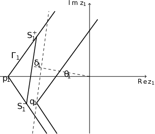
3.1 A calculation relating to figure 3 on page 3.

We justify that the length on interval |0​c||0c| in figure 3 on page 3 indeed equals C1.C_{1}. Observing the three triangles 0​q​a,0​q​b,0​q​c0qa,0qb,0qc we have

R​e​(q​ei​α1)=−|0​a|,\displaystyle Re\left(qe^{i\alpha_{1}}\right)=-|0a|, (3.1.1)
R​e​(q​e−i​α1)=−|0​b|,\displaystyle Re\left(qe^{-i\alpha_{1}}\right)=-|0b|,
R​e​(q​ei​θ1)=−|0​c|.\displaystyle Re\left(qe^{i\theta_{1}}\right)=-|0c|.

Denote x=R​e​(q),y=I​m​(q).x=Re(q),y=Im(q). Then we can paraphrase (3.1.1) as

x​cos⁡(α1)−y​sin⁡(α1)=−A1+,\displaystyle x\cos\left(\alpha_{1}\right)-y\sin\left(\alpha_{1}\right)=-A^{+}_{1},
x​cos⁡(α1)+y​sin⁡(α1)=−A1−,\displaystyle x\cos\left(\alpha_{1}\right)+y\sin\left(\alpha_{1}\right)=-A^{-}_{1},
x​cos⁡(θ1)−y​sin⁡(θ1)=−|[0​c]|.\displaystyle x\cos\left(\theta_{1}\right)-y\sin\left(\theta_{1}\right)=-|[0c]|.

So that

|0​c|=A1+2​[sin⁡(θ1)sin⁡(α1)+cos⁡(θ1)cos⁡(α1)]+A1−2​[cos⁡(θ1)cos⁡(α1)−sin⁡(θ1)sin⁡(α1)].|0c|=\frac{A^{+}_{1}}{2}\left[\frac{\sin\left(\theta_{1}\right)}{\sin\left(\alpha_{1}\right)}+\frac{\cos\left(\theta_{1}\right)}{\cos\left(\alpha_{1}\right)}\right]+\frac{A^{-}_{1}}{2}\left[\frac{\cos\left(\theta_{1}\right)}{\cos\left(\alpha_{1}\right)}-\frac{\sin\left(\theta_{1}\right)}{\sin\left(\alpha_{1}\right)}\right].

Consequently, due to 1.1.3 we have |0​c|=C1.|0c|=C_{1}.

Refer to caption
Figure 3: Construction of C1C_{1}

3.2 An auxiliary estimate.

We now estimate the integral

∫Λ1e−R​e​(ω1​z1)​|d​ω1|,for ​arg⁡(z1)=θ1,\int_{\Lambda_{1}}e^{-Re\left(\omega_{1}z_{1}\right)}\left|d\omega_{1}\right|,\quad\text{for }\arg\left(z_{1}\right)=\theta_{1}, (3.2.1)

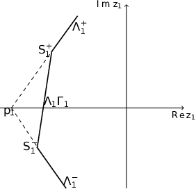
where the curve Λ1\Lambda_{1} is defined by figure 4 on page 4. Due to the choice 1.1.3 of the constant C1C_{1} and parametrization (1.1.8) of the curve Γ1,\Gamma_{1}, the curve Λ1\Lambda_{1} is a union of three subcurves: the finite segment Λ1∖Γ1¯\overline{\Lambda_{1}\setminus\Gamma_{1}} and two infinite segments Λ1+\Lambda_{1}^{+} and Λ1−\Lambda_{1}^{-} correspondingly parameterized by

γ1​(t),t≥t+>0,\displaystyle\gamma_{1}(t),\quad t\geq t_{+}>0, (3.2.2)
γ1​(t),t≤t−<0,\displaystyle\gamma_{1}(t),\quad t\leq t_{-}<0,

where t+t_{+} and t−t_{-} are determined by s−=γ1​(t−),s+=γ1​(t+).s_{-}=\gamma_{1}(t_{-}),s_{+}=\gamma_{1}(t_{+}).

Refer to caption
Refer to caption
Figure 4: Construction of Λ1\Lambda_{1}

Step 1.

Note that due to the choice 1.1.3 of the constant C1,C_{1},

R​e​(ω1​z1)=R​e​(ω1​ei​θ1)​|z1|=−(C1+δ)​|z1|,for ​ω1∈Λ1∖Γ1¯,arg⁡(z1)=θ1.Re\left(\omega_{1}z_{1}\right)=Re\left(\omega_{1}e^{i\theta_{1}}\right)\left|z_{1}\right|=-\left(C_{1}+\delta\right)\left|z_{1}\right|,\quad\text{for }\omega_{1}\in\bar{\Lambda_{1}\setminus\Gamma_{1}},\;\arg\left(z_{1}\right)=\theta_{1}. (3.2.3)

And consequently

∫Λ1∖Γ1e−R​e​(ω1​z1)​|𝑑ω|=e(C1+δ)​|z1|​|Λ1∖Γ1|.\int_{\Lambda_{1}\setminus\Gamma_{1}}e^{-Re\left(\omega_{1}z_{1}\right)}\left|d\omega\right|=e^{\left(C_{1}+\delta\right)\left|z_{1}\right|}\left|\Lambda_{1}\setminus\Gamma_{1}\right|. (3.2.4)

Step 2.

We rewrite

∫Λ1+e−R​e​(ω1​z1)​|d​ω1|​=(3.2.2),(1.1.8)​∫t++∞e−R​e​(γ1​(t)​z1)​𝑑t\int_{\Lambda_{1}^{+}}e^{-Re\left(\omega_{1}z_{1}\right)}\left|d\omega_{1}\right|\overset{\eqref{gammapart},\eqref{gamma_1}}{=}\int_{t_{+}}^{+\infty}e^{-Re\left(\gamma_{1}(t)z_{1}\right)}dt (3.2.5)

Note that

|θ1|<α1<π/2.\left|\theta_{1}\right|{<}\alpha_{1}{<}\pi/2.

Consequently

R​e​(i​e−i​α1​z1)>0,for ​arg⁡(z1)=θ1.Re\left(ie^{-i\alpha_{1}}z_{1}\right)>0,\quad\text{for }\arg\left(z_{1}\right)=\theta_{1}.

So that the following integral is convergent and equals

∫t++∞e−R​e​(γ1​(t)​z1)​𝑑t=e−R​e​(γ1​(t+)​z1)R​e​(i​e−i​α1​z1),for ​arg⁡(z1)=θ1.\int_{t_{+}}^{+\infty}e^{-Re\left(\gamma_{1}(t)z_{1}\right)}dt=\frac{e^{-Re\left(\gamma_{1}\left(t_{+}\right)z_{1}\right)}}{Re\left(ie^{-i\alpha_{1}}z_{1}\right)},\quad\text{for }\arg\left(z_{1}\right)=\theta_{1}. (3.2.6)

Note that γ1​(t+)∈Λ1∖Γ1¯.\gamma_{1}(t_{+})\in\overline{\Lambda_{1}\setminus\Gamma_{1}}. Consequently, due to (3.2.3), we have

R​e​(γ1​(t+)​z1)=−(C1+δ)​|z1|,for ​arg⁡(z1)=θ1.Re\left(\gamma_{1}\left(t_{+}\right)z_{1}\right)=-\left(C_{1}+\delta\right)\left|z_{1}\right|,\quad\text{for }\arg\left(z_{1}\right)=\theta_{1}. (3.2.7)

By combining (3.2.5),(3.2.6),(3.2.7) we get

∫Λ1+e−R​e​(ω1​z1)​|d​ω1|≤e(C1+δ)​|z1|R​e​(i​e−i​α1​z1),for ​arg⁡(z1)=θ1.\int_{\Lambda_{1}^{+}}e^{-Re\left(\omega_{1}z_{1}\right)}\left|d\omega_{1}\right|\leq\frac{e^{\left(C_{1}+\delta\right)\left|z_{1}\right|}}{Re\left(ie^{-i\alpha_{1}}z_{1}\right)},\quad\text{for }\arg\left(z_{1}\right)=\theta_{1}. (3.2.8)

Similarly,

∫Λ1−e−R​e​(ω1​z1)​|d​ω1|≤e(C1+δ)​|z1|R​e​(−i​ei​α1​z1),for ​arg⁡(z1)=θ1.\int_{\Lambda_{1}^{-}}e^{-Re\left(\omega_{1}z_{1}\right)}\left|d\omega_{1}\right|\leq\frac{e^{\left(C_{1}+\delta\right)\left|z_{1}\right|}}{Re\left(-ie^{i\alpha_{1}}z_{1}\right)},\quad\text{for }\arg\left(z_{1}\right)=\theta_{1}. (3.2.9)

Step 3.

By combining the estimates (3.2.4),(3.2.8),(3.2.9), we get

∫Λ1e−R​e​(ω1​z1)​|d​ω1|≤kα1,θ1​e(C1+δ)​|z1||z1|,for ​arg⁡(z1)=θ1,\int_{\Lambda_{1}}e^{-Re\left(\omega_{1}z_{1}\right)}\left|d\omega_{1}\right|\leq k_{\alpha_{1},\theta_{1}}\frac{e^{\left(C_{1}+\delta\right)\left|z_{1}\right|}}{\left|z_{1}\right|},\quad\text{for }\arg\left(z_{1}\right)=\theta_{1}, (3.2.10)

where the number kα1,θ1,k_{\alpha_{1},\theta_{1}}, while depending on α\alpha and θ,\theta, does not depend on |z|.|z|. We remark that the estimate (3.2.10) that we have obtained is similar to the one in lemma 3.1 [2].

3.3 Proof of trigonometric convexity.

As the function mm is analytic on the set Ω1×Ω2,\Omega_{1}\times\Omega_{2}, by consecutive applications of the Cauchy integral theorem in variables z1z_{1} and z2,z_{2}, we can rewrite (1.1.13) as

f⁡(z1,z2)=∫Λ1∫Λ2m⁡(ω1,ω2)​e−ω1​z1−ω2​z2​d​ω2​d​ω1,f\left(z_{1},z_{2}\right)=\int_{\Lambda_{1}}\int_{\Lambda_{2}}m\left(\omega_{1},\omega_{2}\right)e^{-\omega_{1}z_{1}-\omega_{2}z_{2}}d\omega_{2}d\omega_{1}, (3.3.1)

where the curve Λ1\Lambda_{1} is constructed by figure 4 on page 4. Due to construction of the curve Λ1,\Lambda_{1}, it is bounded away from the boundary ∂Ω1.\partial\Omega_{1}. Similarly, the curve Λ2\Lambda_{2} is bounded away from the boundary ∂Ω2.\partial\Omega_{2}. Consequently, due remark 2.1.1, the function mm is uniformly bounded (by some constant kδ​(m)k_{\delta}(m)) on the Cartesian product Λ1×Λ2.\Lambda_{1}\times\Lambda_{2}. We estimate

|f⁡(z1,z2)|​≤(1.1.13)​∫Λ1∫Λ2|m⁡(ω1,ω2)|​e−R​e​(ω1​z1)−R​e​(ω2​z2)​|d​ω2|​|d​ω1|≤\displaystyle\left|f\left(z_{1},z_{2}\right)\right|\overset{\eqref{ivanov_formula}}{\leq}\int_{\Lambda_{1}}\int_{\Lambda_{2}}\left|m\left(\omega_{1},\omega_{2}\right)\right|e^{-Re(\omega_{1}z_{1})-Re\left(\omega_{2}z_{2}\right)}\left|d\omega_{2}\right|\left|d\omega_{1}\right|\leq (3.3.2)
≤(2.1.2)​kδ​(m)​[∫Λ1e−R​e​(ω1​z1)​|d​ω1|]⋅[∫Λ2e−R​e​(ω2​z2)​|d​ω2|]≤\displaystyle\overset{\eqref{mestimate}}{\leq}k_{\delta}(m)\left[\int_{\Lambda_{1}}e^{-Re(\omega_{1}z_{1})}\left|d\omega_{1}\right|\right]\cdot\left[\int_{\Lambda_{2}}e^{-Re\left(\omega_{2}z_{2}\right)}\left|d\omega_{2}\right|\right]\leq
≤(3.2.10)​kδ​(m)​kα1,θ1​kα2,θ2​e(C1+δ)​|z1||z1|​e(C2+δ)​|z2||z2|,\displaystyle\overset{\eqref{step31}}{\leq}k_{\delta}(m)k_{\alpha_{1},\theta_{1}}k_{\alpha_{2},\theta_{2}}\frac{e^{\left(C_{1}+\delta\right)\left|z_{1}\right|}}{\left|z_{1}\right|}\frac{e^{\left(C_{2}+\delta\right)\left|z_{2}\right|}}{\left|z_{2}\right|},
for ​arg⁡(z1)=θ1,arg⁡(z2)=θ2.\displaystyle\quad\text{for }\arg\left(z_{1}\right)=\theta_{1},\;\arg\left(z_{2}\right)=\theta_{2}.

Additionally, due to the estimate (1.1.5) the function ff is bounded in: the intersection of Ω1×Ω2,\Omega_{1}\times\Omega_{2}, and a vicinity of 0.0. By combining this fact with the estimate (3.3.2), we obtain the following estimate on the function f:f:

|f⁡(z1,z2)|≤kδ,θ1,θ2,α1,α2​e(C1+δ)​|z1|+(C2+δ)​|z2|,\displaystyle\left|f\left(z_{1},z_{2}\right)\right|\leq k_{\delta,\theta_{1},\theta_{2},\alpha_{1},\alpha_{2}}e^{(C_{1}+\delta)\left|z_{1}\right|+\left(C_{2}+\delta\right)\left|z_{2}\right|},
for ​arg⁡(z1)=θ1,arg⁡(z2)=θ2,\displaystyle\text{for }\arg\left(z_{1}\right)=\theta_{1},\;\arg\left(z_{2}\right)=\theta_{2},

where the constant kδ,θ1,θ2,α1,α2,k_{\delta,\theta_{1},\theta_{2},\alpha_{1},\alpha_{2}}, while depending on δ,θ1,θ2,α1,α2,\delta,\theta_{1},\theta_{2},\alpha_{1},\alpha_{2}, does not depend on |z1|\left|z_{1}\right| or |z2|.\left|z_{2}\right|.

4 Proof of sharpness.

Consider the entire function f⁡(z1,z2)=ez1+z2.f(z_{1},z_{2})=e^{z_{1}+z_{2}}. The function ff is of exponential type,

|f(z1,z2)|≤e|z1|cosθ1+|z2|cosθ2,for z1,z2∈ℂ.\left|f\left(z_{1},z_{2}\right)\right|\leq e^{\left|z_{1}\right|\cos\theta_{1}+\left|z_{2}\right|\cos\theta_{2}},\quad\text{for }z_{1},z_{2}\in\mathbb{C}.

For our choice of the function f,f, the set Tf​(θ1,θ2)T_{f}(\theta_{1},\theta_{2}) defined by (1.1.2) equals

Tf(θ1,θ2)={(ν1,ν2):ν1≥cosθ1,ν2≥cosθ2}\displaystyle T_{f}\left(\theta_{1},\theta_{2}\right)=\left\{(\nu_{1},\nu_{2}):\nu_{1}\geq\cos\theta_{1},\nu_{2}\geq\cos\theta_{2}\right\} (4.0.1)

(see figure 5 on page 5).

Refer to caption
Figure 5: Tf​(θ1,θ2)T_{f}\left(\theta_{1},\theta_{2}\right)

In particular, for α1=α2=±π4\alpha_{1}=\alpha_{2}=\pm\frac{\pi}{4} we have

Tf(±π4,±π4)={(ν1,ν2):ν1≥22,ν2≥22}.T_{f}\left(\pm\frac{\pi}{4},\pm\frac{\pi}{4}\right)=\left\{(\nu_{1},\nu_{2})\colon\nu_{1}\geq\frac{\sqrt{2}}{2},\nu_{2}\geq\frac{\sqrt{2}}{2}\right\}.

Thus

A1+=A2+=A1−=A2−=22.A^{+}_{1}=A^{+}_{2}=A^{-}_{1}=A^{-}_{2}=\frac{\sqrt{2}}{2}.

Take θ1=θ2=0.\theta_{1}=\theta_{2}=0. By (1.1.3) we evaluate

C1=C2=24​22+24​22=1.C_{1}=C_{2}=\frac{\sqrt{2}}{4}\frac{2}{\sqrt{2}}+\frac{\sqrt{2}}{4}\frac{2}{\sqrt{2}}=1.

Thus, according to theorem 1.1.5 the following inequality holds:

f⁡(z1,z2)≤kε​e(1+ε)​|z1|+(1+ε)​|z2|,for ​arg⁡z1=arg⁡z2=0.f(z_{1},z_{2})\leq k_{\varepsilon}e^{(1+\varepsilon)\left|z_{1}\right|+(1+\varepsilon)\left|z_{2}\right|},\quad\text{for }\arg z_{1}=\arg z_{2}=0.

On the other hand, by (4.0.1)

Tf(0,0)={(ν1,ν2):ν1≥1,ν2≥1}.T_{f}(0,0)=\left\{(\nu_{1},\nu_{2}):\nu_{1}\geq 1,\nu_{2}\geq 1\right\}.

That is, in this case, theorem 1.1.5 is sharp.

Acknowledgments

The first author was funded by a grant of the Russian Science Foundation (project No. 20-11-20117)

The second author was partially funded by a project of the Russian Ministry of Science and Education for the organization and development of scientific and educational mathematical centers (agreement No. 075-02-2022-893).

References

  • Ivanov [1959] V. Ivanov. A characterization of the growth of an entire function of two variables and its application to the summation of double power series. Mat. Sb. (N.S.), 47(89)(1):3–16, 1959.
  • Vagharshakyan [2022] A. Vagharshakyan. Sectorial paley-wiener theorem, 2022. Preprint at https://arxiv.org/abs/2205.02192.
  • Dzhrbashyan and A. [1960] M. Dzhrbashyan and Avetisyan A. Integral representation of a certain class of functions analytic in an angular domain. Sib. Math. J., 1(3):383–426, 1960.
  • Friot and Greynat [2012] S. Friot and D. Greynat. On convergent series representations of mellin-barnes integrals. J. Math. Phys., 53(023508), 2012. doi: 10.1063/1.3679686.
  • Passare et al. [2000] M. Passare, A. Tsikh, and A. Yger. Residue currents of the bochner-martinelli type. Publ. Mat., 44(1):85–117, 2000.
  • Phragmen and Lindelöf [1908] F. Phragmen and E. Lindelöf. Sur une extension d’un principe classique de l’analyseet sur quelques proprietes des fonctions monogenes dans le voisinage d’un point singulier. Acta Math., 31:381–406, 1908.
  • Bieberbach [1955] L. Bieberbach. Analytische Fortsetzun. Springer-Verlag, Berlin, 1955. doi: 10.1007/978-3-662-01270-3.
  • Levin [1964] B. Levin. Distribution of zeros of entire functions. American Mathematical Society, Providence, R.I., 1964. doi: 10.1090/mmono/005.
  • Boas [1954] R. Boas. Entire Functions. Academic Press, New York, 1954.
  • Pólya [1929] G. Pólya. Untersuchungen über lücken und singularitäten von potenzreihen. Math. Z., 29:549–640, 1929.
  • Carlson [1921] F. Carlson. Uber ganzwertige Funktionen. Math. Z., 11:1–23, 1921.
  • Carlson [1914] F. Carlson. Sur une classe de series de Taylor. Diss. Upsala, Upsala, 1914.
  • Arakelian [1985] N. Arakelian. On efficient analytic continuation of power series. Math. Sb., 52(1):21–39, 1985. doi: 10.1070/SM1985v052n01ABEH002875.
  • Arakelian et al. [2007] N. Arakelian, W. Luh, and J. Muller. On the localization of singularities of lacunar power series. Complex Var. Elliptic Equ., 52(7):561–573, 2007. doi: 10.1080/17476930701246396.
  • Leont’ev [1983] A. Leont’ev. Entire Functions. Exponential Series. Nauka, Moscow, 1983.
  • Ronkin [1974] L. Ronkin. Introduction to the theory of entire functions of several variables. In Transl. Math. Monographs, volume 44, Providence, R.I., 1974. Amer. Math. Soc. doi: 10.1090/mmono/044.
  • Lelong and Gruman [1986] P. Lelong and L. Gruman. Entire functions of several complex variables. Springer, Berlin, 1986. doi: 10.1007/978-3-642-70344-7.
  • Kiselman [1967] C. Kiselman. On entire functions of exponential type and indicators of analytic functionals. Acta Math., 117:1–35, 1967. doi: 10.1007/BF02395038.
  • Kondratyuk [1979] A. Kondratyuk. The fourier series method for entire and meromorphic functions of completely regular growth. Sb. Math., 35(1):63–84, 1979. doi: 10.1070/SM1984v048n02ABEH002677.
  • Malyutin and Sadik [2011] K. Malyutin and N. Sadik. The indicator of a delta-subharmonic function in a half- plane. Ufa Math. J., 3(4):84–91, 2011.
  • Mkrtchyan [2022] A. Mkrtchyan. Continuability of multiple power series into sectorial domain by means of interpolation of coefficients. Ufa Math. J., 14(2):1–8, 2022.

Aleksandr Mkrtchyan

AMkrtchyan@sfu-kras.ru

24/5 Marshal Bagramian ave.

Yerevan, 0019, Republic of Armenia

Armen Vagharshakyan

avaghars@kent.edu

24/5 Marshal Bagramian ave.

Yerevan, 0019, Republic of Armenia