跳到论文正文
W Papers独立论文阅读器 arXiv:2205.02512 论文正文 计算阅读时间 · 0%
引用这篇论文根据当前论文元数据生成,正式投稿前建议核对。


License: arXiv.org perpetual non-exclusive license
arXiv:2205.02512v1 [eess.SP] 05 May 2022

Secure Communication in Multifunctional Active Intelligent Reflection Surface-assisted Systems

Shaokang Hu, Derrick Wing Kwan Ng, and Jinhong Yuan
School of Electrical Engineering and Telecommunications, University of New South Wales, Sydney, Australia
Abstract

In this paper, the secure performance of multiuser multiple-input single-output wireless communications systems assisted by a multifunctional active intelligent reflection surface (IRS) is investigated. The active IRS can simultaneously reflect and amplify the incident signals and emit artificial noise to combat potential wiretapping. We minimize the total system power consumption by designing the phase, amplitude, and IRS mode selection of the active IRS elements, as well as the precoder and artificial noise vector of the base station (BS). The design is formulated as a non-convex optimization problem guaranteeing communication security. To tackle the problem, this paper proposes an iterative alternating algorithm to obtain an effective sub-optimal solution. The simulation results show that the proposed scheme offers superior secure performance over all the considered baseline schemes, especially when the number of eavesdropper antennas is more than that of the BS.

I Introduction

With the rapid development of meta-materials and electromagnetic materials, passive intelligent reflecting surfaces (IRSs) have been advocated as a promising solution to enable future wireless communications as they provide a new degrees-of-freedom (DoF) to intelligently shape the propagation condition of wireless channels [1]. However, the performance of passive IRS-assisted systems is constrained by the inherent “double-fading” attenuation. In particular, since the received signals propagate through the cascaded reflection link, they suffer severe attenuation from large-scale fading twice[2]. To circumvent this challenge, active IRS has been proposed in [3, 4, 5]. Different from passive IRSs, active reflection-type amplifiers are integrated into each element of active IRSs that can be realized by off-the-shelf components such as current-inverting converters[6]. As a result, an active IRS can further amplify the incident signals with controllable amplitudes and phases to mitigate the impacts of large-scale fading. Nevertheless, one major drawback of active IRS is that its associated noise power, e.g. thermal noise, scales with the transmit power of the active IRS that may result in a system performance bottleneck[3].

On the other hand, although IRSs can improve the received signal strength, it also increases the susceptibility to potential eavesdropping. As a result, in IRS-assisted wireless communications, communication security is a critical concern [7]. To realize secure communication, numerous works have adopted the physical layer security techniques, e.g. artificial noise (AN)-aided beamforming[8]. Conventionally, a properly designed AN signal is inserted into the transmitted signals by the base station (BS) deliberately to confuse the signal detection at potential eavesdroppers. The rationale behind the AN design is to effectively reduce the interference leakage to the legitimate users while degrading the intercepted signal quality at the potential eavesdroppers via optimizing the direction of AN. As such, the BS is able to improve the secrecy performance by adaptively adjusting the spatial directions of AN and the information signals jointly via spatial beamforming[8]. Unfortunately, this technique can only guarantee communication security when the total number of antennas equipped at the transmitter is larger than the receive ones at the eavesdropper. For this reason, most of the existing works, e.g. [7, 9], ideally assume that the number of eavesdropper antennas is less than that of the BS even though it may not hold in practice. To overcome the aforementioned difficulties, this paper designs secure communication systems assisted by a multifunctional active IRS with the ability to emit AN to combat potential wiretapping. In particular, the originally detrimental thermal noise at the active IRS is exploited as beneficial AN for secrecy communication provisioning. Thus, effective secure communications can be obtained even when the number of eavesdroppers’ antennas has a competitive edge over the BS.

In this paper, we formulate the resource allocation algorithm design for active IRS-assisted multiuser multiple-input single-output (MISO) wireless systems with the presence of a multi-antenna eavesdropper to minimize the total system power consumption. In contrast to previously published works [3, 4, 5], this paper is the first attempt to propose a novel versatile active IRS to realize secure wireless communications. In particular, this work allows each active IRS element operating in either the reflection mode or the jamming mode to swing the balance between improving the signal quality of the users and communication security. By smartly optimizing the IRS mode selection, phase and amplitude of active IRS elements, and the precoder and AN vector of the BS, the active IRS can adaptively serve as a separate jamming source against potential eavesdropping, while reflecting the impinging signals to the desired legitimate users. To handle the challenging non-convex optimization problem, we propose an alternating optimization (AO)-based algorithm to obtain an effective sub-optimal solution. Simulation results show that the proposed scheme outperforms all the baseline schemes, especially when the number of eavesdroppers’ antenna is larger than that of the BS.

Notations: Lowercase letter xx, boldface lowercase letter 𝐱\mathbf{x}, and boldface uppercase letter 𝐗\mathbf{X} are used to denote scalars, vectors, and matrices, respectively. The space of N×MN\times M real, complex, and binary matrices are denoted by ℝN×M\mathbb{R}^{N\times M}, ℂN×M\mathbb{C}^{N\times M}, and 𝔹N×M\mathbb{B}^{N\times M}, respectively. An N×NN\times N Hermitian matrix is represented by ℍN\mathbb{H}^{N}. |⋅||\cdot|, ∥⋅∥\|\cdot\|, and ∥⋅∥F\|\cdot\|_{\mathrm{F}} denote the modulus of a complex-valued scalar, an Euclidean norm of a vector, and Frobenius norm of a matrix, respectively. λmax​(⋅)\lambda_{\max}(\cdot), det⁡(⋅)\mathrm{det}(\cdot), (⋅)T(\cdot)^{\mathrm{T}}, (⋅)H(\cdot)^{\mathrm{H}}, (⋅)∗(\cdot)^{*}, 𝔼​{⋅}\mathbb{E}\{\cdot\}, Rank⁡(⋅)\mathrm{Rank}(\cdot), and Tr⁡(⋅)\mathrm{Tr(\cdot)} represent the largest eigenvalue, determinant, transpose, conjugate transpose, conjugate, expectation, rank, and trace of a matrix, respectively. [x]+=max⁡{0,x}[x]^{+}=\max\{0,x\}. Positive semi-definite of matrix 𝐗\mathbf{X} is represented by 𝐗⪰𝟎\mathbf{X}\succeq\mathbf{0}. diag⁡(𝐱)\mathrm{diag(\mathbf{x})} or diag~​(𝐗)\widetilde{\mathrm{diag}}(\mathbf{X}) denote a diagonal matrix whose entry is vector 𝐱\mathbf{x} or identical to that of 𝐗\mathbf{X}, respectively. 𝒞​𝒩​(μ,σ2)\mathcal{CN}(\mu,\sigma^{2}) denotes the distribution of a circularly symmetric complex Gaussian (CSCG) random variable with mean μ\mu and variance σ2\sigma^{2}, where ∼\sim represents “distributed as”. 𝐈N\mathbf{I}_{N} stands for an N×NN\times N identity matrix.

II System Model

Refer to caption
Fig. 1: A secure wireless communication system with a multifunctional active IRS, a multi-antenna eavesdropper (Eve), and KK users.

The considered secure transmission system, shown in Fig. 1, consists of four types of nodes, i.e., a base station (BS) with NTN_{\mathrm{T}} antennas, KK single-antenna users, an active IRS with MM elements, and an eavesdropper with NEN_{\mathrm{E}} antennas11 1 The consideration of an eavesdropper with multiple antennas is equivalent to the case of cooperative multiple single-antenna eavesdroppers[10]., where M+NT≥NEM+N_{\mathrm{T}}\geq N_{\mathrm{E}}. Specifically, the BS intends to transmit confidential information to the KK users simultaneously. To enhance the communication security, both the BS and the active IRS are able to emit jamming signals to combat potential wiretapping. A quasi-static flat fading channel model [4, 7] is assumed and the channel state information (CSI) of all the channels is assumed to be perfectly known, which can be achieved by currently available channel estimation methods22 2 To obtain intuitive insights, we assume a perfect CSI model in this paper. The case of the imperfect CSI model will be considered in its journal version. [11]. The baseband equivalent channels from the BS to the active IRS (BS-IRS), from the active IRS to user kk (IRS-userk), from the active IRS to the eavesdropper (IRS-Eve), from the BS to user kk (BS-userk), and from the BS to the eavesdropper (BS-Eve) are denoted by 𝐆∈ℂM×NT\bm{\mathbf{G}}\in\mathbb{C}^{M\times N_{\mathrm{T}}}, 𝐡IU,kH∈ℂ1×M\mathbf{h}_{\mathrm{IU},k}^{\mathrm{H}}\in\mathbb{C}^{1\times M}, 𝐇IE∈ℂNE×M\mathbf{H}_{\mathrm{IE}}\in\mathbb{C}^{N_{\mathrm{E}}\times M}, 𝐡BU,kH∈ℂ1×NT\mathbf{h}_{\mathrm{BU},k}^{\mathrm{H}}\in\mathbb{C}^{1\times N_{\mathrm{T}}}, and 𝐇BE∈ℂNE×NT\mathbf{H}_{\mathrm{BE}}\in\mathbb{C}^{N_{\mathrm{E}}\times N_{\mathrm{T}}}, respectively.

II-A Signal Model

II-A1 Transmitted Signal at the BS

The transmitted signal from the BS is given by

𝐱=∑k=1K𝐰k​xk+𝐳B,\displaystyle\mathbf{x}=\sum_{k=1}^{K}\mathbf{w}_{k}x_{k}+\mathbf{z}_{\mathrm{B}}, (1)

where 𝐰k∈ℂNT×1,∀k∈{1,…,K}\mathbf{w}_{k}\in\mathbb{C}^{N_{\mathrm{T}}\times 1},\forall k\in\{1,\ldots,K\}, is the precoding vector for user kk and xk∼𝒞​𝒩​(0,1)x_{k}\sim\mathcal{CN}(0,1) is the data symbol intended for user kk. The AN vector is represented by 𝐳B∈ℂNt×1\mathbf{z}_{\mathrm{B}}\in\mathbb{C}^{N_{\mathrm{t}}\times 1} which is generated by the BS to deliberately combat the eavesdropper. Specifically, 𝐳B\mathbf{z}_{\mathrm{B}} is a CSCG vector with 𝐳B∼𝒞​𝒩​(𝟎,𝐙B)\mathbf{z}_{\mathrm{B}}\sim\mathcal{CN}(\mathbf{0},\mathbf{Z}_{\mathrm{B}}), where 𝐙B=𝔼⁡{𝐳B​𝐳BH}\mathbf{Z}_{\mathrm{B}}=\mathbb{E}\{\mathbf{z}_{\mathrm{B}}\mathbf{z}_{\mathrm{B}}^{\mathrm{H}}\} is the covariance matrix of the AN vector. Notably, the AN is supposed to be unknown to both the legitimate users and the potential eavesdropper and the proposed algorithm will optimize the AN to facilitate communication security provisioning in the next section.

II-A2 Reflected Signal at the IRS

As shown in Fig. 1, some of the elements in the active IRS are selected for emitting jamming signals and the rest reflecting the impinging signals to the users. In particular, the reflection matrix of the IRS is denoted as 𝐀​𝚯\mathbf{A}\bm{\Theta}. Matrix 𝚯=diag⁡(ϕ)∈ℂM×M\bm{\Theta}=\mathrm{diag}(\bm{\phi})\in\mathbb{C}^{M\times M}, where ϕ=[ϕ1,…,ϕm,…,ϕM]T∈ℂM×1\bm{\phi}=[\phi_{1},\ldots,\phi_{m},\ldots,\phi_{M}]^{\mathrm{T}}\in\mathbb{C}^{M\times 1} and ϕm=pm​ej​θm\phi_{m}=p_{m}e^{j\theta_{m}}, ∀m∈[1,…,M]\forall m\in[1,\ldots,M], is a diagonal matrix, which controls the phase shifts and amplitude gain introduced by the active IRS. Besides, θm∈[0,2​π)\theta_{m}\in[0,2\pi) and pm≥0p_{m}\geq 0 are the phase shift and the amplitude coefficient for the mm-th active IRS element, respectively. Thanks to the integrated active amplifier, pmp_{m} can be lager than one as in contrast to its counterpart in passive IRSs, e.g. [3, 4, 5]. Also, 𝐀=diag⁡(𝜶)∈𝔹M×M\mathbf{A}=\mathrm{diag}(\bm{\alpha})\in\mathbb{B}^{M\times M} is a mode selection matrix that to be optimized, where 𝜶=[α1,…,αm,…,αM]T∈𝔹M×1\bm{\alpha}=[\alpha_{1},\ldots,\alpha_{m},\ldots,\alpha_{M}]^{\mathrm{T}}\in\mathbb{B}^{M\times 1}. Binary variable αm∈{0,1}\alpha_{m}\in\{0,1\}, is an IRS mode selector, which is defined as:

αm={1,Reflection mode at the active IRS element​m​,0,Jamming mode at the active IRS element​m​.\displaystyle\hskip-8.53581pt\alpha_{m}\hskip-2.84526pt=\hskip-2.84526pt\left\{\begin{array}[]{ll}\hskip-5.69054pt1,&\hskip-5.69054pt\text{Reflection mode at the active IRS element}\,m\text{,}\\ \hskip-5.69054pt0,&\hskip-5.69054pt\text{Jamming mode at the active IRS element}\,m\text{.}\end{array}\right.
Fig. 2: An architecture of the proposed active IRS[3, 12].

As shown in Fig. 2, each of the active IRS elements can be set in either the reflection mode or the jamming mode. Specifically, active IRS elements in the reflection mode amplify and reflect all impinging signals, while the elements in the jamming mode generate a power-normalized AN and then amplify it to degrade the received signal quality of the eavesdropper. Moreover, the power budget of the active IRS is limited to ‖𝚯‖F2≤PImax\|\bm{\Theta}\|^{2}_{\mathrm{F}}\leq P_{\mathrm{I}}^{\max}, where PImaxP_{\mathrm{I}}^{\max} is a constant.

Therefore, the overall signal processing model at the proposed active IRS is given as

𝐲I=𝐀​𝚯​𝐆𝐱⏟Desired signal+(𝐈M−𝐀)​𝚯​𝐳I⏟AN+𝚯​𝐧I⏟Dynamic noise+𝐧s⏟Static noise,\displaystyle\mathbf{y}_{\mathrm{I}}\hskip-2.84526pt=\hskip-2.84526pt\underbrace{\mathbf{A}\mathbf{\Theta}\mathbf{G}\mathbf{x}}_{\text{Desired signal}}+\underbrace{(\mathbf{I}_{M}-\mathbf{A})\mathbf{\Theta}\mathbf{z}_{\mathrm{I}}}_{\text{AN}}+\underbrace{\bm{\Theta}\mathbf{n}_{\mathrm{I}}}_{\text{Dynamic noise}}+\underbrace{\cancel{\mathbf{n}_{\mathrm{s}}}}_{\text{Static noise}}, (4)

where 𝐳I∈ℂM×1\mathbf{z}_{\mathrm{I}}\in\mathbb{C}^{M\times 1} denotes the power-normalized AN vector generated by the active IRS and 𝔼⁡{𝐳I​𝐳IH}=𝐈M\mathbb{E}\{\mathbf{z}_{\mathrm{I}}\mathbf{z}_{\mathrm{I}}^{\mathrm{H}}\}=\mathbf{I}_{M}. As shown in (4), the power of the dynamic noise 𝚯​𝐧I\mathbf{\Theta}\mathbf{n}_{\mathrm{I}} is scaled with the power gain introduced by the active IRS, where 𝐧I\mathbf{n}_{\mathrm{I}} is introduced by the input noise and inherent device noise. We model 𝐧I∈ℂM×1\mathbf{n}_{\mathrm{I}}\in\mathbb{C}^{M\times 1} as 𝐧I∼𝒞​𝒩​(𝟎M,σI2​𝐈M)\mathbf{n}_{\mathrm{I}}\sim\mathcal{CN}(\mathbf{0}_{M},\sigma_{\mathrm{I}}^{2}\mathbf{I}_{M}), where σI2≥0\sigma_{\mathrm{I}}^{2}\geq 0 is the corresponding power. Note that by optimizing 𝚯\mathbf{\Theta}, the inherent noise generated by the active IRS, i.e., 𝚯​𝐧I\mathbf{\Theta}\mathbf{n}_{\mathrm{I}}, can also serve as a jamming source to combat eavesdropping, rather than only being an interference to the system. On the other hand, different from the dynamic noise, the static noise 𝐧s\mathbf{n}_{\mathrm{s}} is independent of amplification factors and it is usually negligible small compared with the dynamic noise[13]. As such, for simplicity, it is neglected in the sequel.

II-A3 Signal Model of Users

The received signal at user kk, ∀k\forall k, can be modeled as

yU,k=𝐡BU,kH​𝐱+𝐡IU,kH​𝐲I+nU,k,\displaystyle y_{\mathrm{U},k}=\mathbf{h}_{\mathrm{BU},k}^{\mathrm{H}}\mathbf{x}+\mathbf{h}_{\mathrm{IU},k}^{\mathrm{H}}\mathbf{y}_{\mathrm{I}}+n_{\mathrm{U},k}, (5)

where the thermal noise at user kk is represented by nU,k∼𝒞​𝒩​(0,σU,k2)n_{\mathrm{U},k}\sim\mathcal{CN}(0,\sigma^{2}_{\mathrm{U},k}). Therefore, the achievable rate and the signal-to-interference-plus-noise ratio (SINR) at user kk, ∀k\forall k, are

RU,k=\displaystyle R_{\mathrm{U},k}\hskip-2.84526pt= log2⁡(1+γU,k)​ and\displaystyle\log_{2}(1+\gamma_{\mathrm{U},k})\text{ and} (6)
γU,k=\displaystyle\gamma_{\mathrm{U},k}\hskip-2.84526pt= |𝐡eq,kH​𝐰k|2μk+|𝐡IU,kH​(𝐈M−𝐀)​𝚯|2+σI2​Tr​(𝐡IU,kH​𝚯​𝚯H​𝐡IU,k),\displaystyle\frac{|\mathbf{h}_{\mathrm{eq},k}^{\mathrm{H}}\mathbf{w}_{k}|^{2}}{\mu_{k}\hskip-2.84526pt+\hskip-2.84526pt|\mathbf{h}_{\mathrm{IU},k}^{\mathrm{H}}(\mathbf{I}_{M}\hskip-2.84526pt-\hskip-2.84526pt\mathbf{A})\mathbf{\Theta}|^{2}\hskip-2.84526pt+\hskip-2.84526pt\sigma_{\mathrm{I}}^{2}\mathrm{Tr}(\mathbf{h}_{\mathrm{IU},k}^{\mathrm{H}}\bm{\Theta}\bm{\Theta}^{\mathrm{H}}\mathbf{h}_{\mathrm{IU},k})},

respectively, where μk=Tr⁡(𝐡eq,kH​(∑j≠kK𝐰j​𝐰jH+𝐙B)​𝐡eq,k)+σU,k2\mu_{k}=\mathrm{Tr}(\mathbf{h}_{\mathrm{eq},k}^{\mathrm{H}}(\sum_{j\neq k}^{K}\mathbf{w}_{j}\mathbf{w}_{j}^{\mathrm{H}}+\mathbf{Z}_{\mathrm{B}})\mathbf{h}_{\mathrm{eq},k})+\sigma^{2}_{\mathrm{U},k} and 𝐡eq,kH=𝐡BU,kH+𝐡IU,kH​𝐀​𝚯​𝐆,∀k\mathbf{h}_{\mathrm{eq},k}^{\mathrm{H}}=\mathbf{h}_{\mathrm{BU},k}^{\mathrm{H}}+\mathbf{h}_{\mathrm{IU},k}^{\mathrm{H}}\mathbf{A}\mathbf{\Theta}\mathbf{G},\forall k.

II-A4 Signal Model of the Eavesdropper

The received signal at the eavesdropper is given by

𝐲E=\displaystyle\mathbf{y}_{\mathrm{E}}= 𝐇BE​𝐱+𝐇IE​𝐲I+𝐧E.\displaystyle\mathbf{H}_{\mathrm{BE}}\mathbf{x}+\mathbf{H}_{\mathrm{IE}}\mathbf{y}_{\mathrm{I}}+\mathbf{n}_{\mathrm{E}}. (7)

Since the capability of the eavesdropper is unknown to the BS, for security provisioning, we assume that the eavesdropper has unlimited computational resources and is thus capable of cancelling all multiuser interference prior to decoding the information of a potential user. Besides, the thermal noise 𝐧E\mathbf{n}_{\mathrm{E}} at the eavesdropper is ignored as it is also unknown to the BS. These worst-case assumptions lead to an upper bound on the channel capacity between the BS and the eavesdropper for decoding the signal of legitimate user kk [9], which is given

CE,k=\displaystyle{C}_{\mathrm{E},k}\hskip-2.84526pt= log2⁡(det(𝐈NE+𝐐−1​𝐅eq​𝐰k​𝐰kH​𝐅eqH)),∀k,\displaystyle\log_{2}\Big(\det\big(\mathbf{I}_{N_{\mathrm{E}}}+\mathbf{Q}^{-1}\mathbf{F}_{\mathrm{eq}}\mathbf{w}_{k}\mathbf{w}_{k}^{\mathrm{H}}\mathbf{F}_{\mathrm{eq}}^{\mathrm{H}}\big)\Big),\forall k, (8)
𝐐=\displaystyle\mathbf{Q}\hskip-2.84526pt= 𝐅eq​𝐙B​𝐅eqH+𝐇IE​(𝐈M−𝐀)​𝚯​𝚯H​𝐇IEH+σI2​𝐇IE​𝚯​𝚯H​𝐇IEH,\displaystyle\mathbf{F}_{\mathrm{eq}}\mathbf{Z}_{\mathrm{B}}\mathbf{F}_{\mathrm{eq}}^{\mathrm{H}}\hskip-2.84526pt+\hskip-2.84526pt\mathbf{H}_{\mathrm{IE}}(\mathbf{I}_{M}\hskip-2.84526pt-\hskip-2.84526pt\mathbf{A})\mathbf{\Theta}\mathbf{\Theta}^{\mathrm{H}}\mathbf{H}_{\mathrm{IE}}^{\mathrm{H}}\hskip-2.84526pt+\hskip-2.84526pt\sigma_{\mathrm{I}}^{2}\mathbf{H}_{\mathrm{IE}}\bm{\Theta}\bm{\Theta}^{\mathrm{H}}\mathbf{H}_{\mathrm{IE}}^{\mathrm{H}},

where 𝐅eq=𝐇BE+𝐇IE​𝐀​𝚯​𝐆\mathbf{F}_{\mathrm{eq}}=\mathbf{H}_{\mathrm{BE}}+\mathbf{H}_{\mathrm{IE}}\mathbf{A}\mathbf{\Theta}\mathbf{G}. Hence, the achievable secrecy rate between the BS and user kk is Rs,k=[RU,k−CE,k]+,∀kR_{\mathrm{s},k}=[R_{\mathrm{U},k}-C_{\mathrm{E},k}]^{+},\forall k.

III Problem Formulation

We aim to minimize the total system power consumption at the BS and the active IRS by jointly designing 𝐰k\mathbf{w}_{k}, 𝐙B\mathbf{Z}_{\mathrm{B}}, αm\alpha_{m}, and 𝚯\mathbf{\Theta}, which can be formulated as optimization problem 𝒫​1\mathcal{P}1:

𝒫​1:\displaystyle\mathcal{P}1:\hskip-8.53581pt minimize𝐰k,𝐙B∈ℍNt,αm,𝚯​∑k=1K‖𝐰k‖2+Tr⁡(𝐙B)+‖𝚯‖F2\displaystyle\underset{\mathbf{w}_{k},\,\mathbf{Z}_{\mathrm{B}}\in\mathbb{H}^{N_{\mathrm{t}}},\,\alpha_{m},\,\mathbf{\Theta}}{\mathrm{minimize}}\,\,\sum_{k=1}^{K}\|\mathbf{w}_{k}\|^{2}+\mathrm{Tr}(\mathbf{Z}_{\mathrm{B}})+\|\mathbf{\Theta}\|^{2}_{\mathrm{F}} (9)
s.t.C1:γU,k≥γkmin,∀k,\displaystyle\mathrm{s.t.}\,\,\mathrm{C1}\hskip-2.84526pt:\gamma_{\mathrm{U},k}\geq\gamma_{k}^{\min},\forall k,
C2:log2⁡(det(𝐈NE+𝐐−1​𝐅eq​𝐰k​𝐰kH​𝐅eqH))≤Ckmax,∀k,\displaystyle\hskip 17.07164pt\mathrm{C2}\hskip-2.84526pt:\log_{2}\Big(\det(\mathbf{I}_{N_{\mathrm{E}}}\!+\!\mathbf{Q}^{-1}\mathbf{F}_{\mathrm{eq}}\mathbf{w}_{k}\mathbf{w}_{k}^{\mathrm{H}}\mathbf{F}_{\mathrm{eq}}^{\mathrm{H}})\Big)\!\leq\!C_{k}^{\max}\!,\forall k,
C3:𝐙B⪰𝟎,C4:αm∈{0,1},∀m,C5:∥𝚯∥2≤PImax.\displaystyle\hskip 17.07164pt\mathrm{C3}\hskip-2.84526pt:\mathbf{Z}_{\mathrm{B}}\succeq\mathbf{\mathbf{0}},\hskip 0.0pt\mathrm{C4}\hskip-2.84526pt:\alpha_{m}\in\{0,1\},\forall m,\mathrm{C5}\hskip-2.84526pt:\|\mathbf{\Theta}\|^{2}\leq P_{\mathrm{I}}^{\max}.

Here, constraint C1\mathrm{C1} ensures the minimum required SINR at user kk such that its achievable rate, i.e., RU,kR_{\mathrm{U},k}, exceeds log2⁡(1+γkmin)\log_{2}(1+\gamma_{k}^{\min}). In constraint C2\mathrm{C2}, the maximum tolerable information leakage to the eavesdropper for wiretapping the signals transmitted to user kk is limited to CkmaxC_{k}^{\max}. By combining C1\mathrm{C1} and C2\mathrm{C2}, the achievable secrecy rate between the BS and user kk is bounded by below, i,e., Rs,k≥[RU,k−Ckmax]+R_{\mathrm{s},k}\geq[R_{\mathrm{U},k}-C_{k}^{\max}]^{+}, such that the minimum required secrecy rate is guaranteed. 𝐙B∈ℍNt\mathbf{Z}_{\mathrm{B}}\in\mathbb{H}^{N_{\mathrm{t}}} and C3\mathrm{C3} guarantees that 𝐙B\mathbf{Z}_{\mathrm{B}} satisfies the requirements of being a covariance matrix of the AN vector. Constraint C4\mathrm{C4} requires that each active IRS element function in one of two modes: reflection mode or jamming mode. Constraint C5\mathrm{C5} limits the power budget of the active IRS under PImaxP_{\mathrm{I}}^{\max}.

IV Optimization Solution

The formulated problem, 𝒫​1\mathcal{P}1, is non-convex due to the binary variable αm\alpha_{m} in constraint C4\mathrm{C4}. Moreover, optimization variables are coupled in constraints C1\mathrm{C1} and C2\mathrm{C2} of the formulated problem 𝒫​1\mathcal{P}1. Generally, obtaining the global optimization solution to 𝒫​1\mathcal{P}1 requires an exhaustive search, which is computational expensive even for moderate system size. Therefore, we present a computationally efficient iterative AO algorithm to obtain a sub-optimal solution to the problem 𝒫​1\mathcal{P}1.

IV-A Problem Transformation

In this section, 𝒫​1\mathcal{P}1 will be first rewritten as its equivalent form 𝒫​2\mathcal{P}2, which paves the way to facilitate the development of the AO method. To start with, we introduce the following proposition to handle the non-convexity of C2\mathrm{C2}.

Proposition 1.

Since 𝐐−12​𝐅eq​𝐰k​𝐰kH​𝐅eqH​𝐐−12\mathbf{Q}^{-\frac{1}{2}}\mathbf{F}_{\mathrm{eq}}\mathbf{w}_{k}\mathbf{w}_{k}^{\mathrm{H}}\mathbf{F}_{\mathrm{eq}}^{\mathrm{H}}\mathbf{Q}^{-\frac{1}{2}} is a rank-one matrix, C2\mathrm{C2} in 𝒫​1\mathcal{P}1 can be equivalently transformed as

C2¯:\displaystyle\overline{\mathrm{C2}}\hskip-2.84526pt: CE,kTol​(𝐅eq​𝐙B​𝐅eqH+𝐇IE​(𝐈M−𝐀)​𝚯​𝚯H​𝐇IEHCLOSE\displaystyle C_{\mathrm{E},k}^{\mathrm{Tol}}\Big(\mathbf{F}_{\mathrm{eq}}\mathbf{Z}_{\mathrm{B}}\mathbf{F}_{\mathrm{eq}}^{\mathrm{H}}\hskip 0.0pt+\hskip 0.0pt\mathbf{H}_{\mathrm{IE}}(\mathbf{I}_{M}\hskip-2.84526pt-\hskip-2.84526pt\mathbf{A})\mathbf{\Theta}\mathbf{\Theta}^{\mathrm{H}}\mathbf{H}_{\mathrm{IE}}^{\mathrm{H}} (10)
OPEN+σI2​𝐇IE​𝚯​𝚯H​𝐇IEH)−𝐅eq​𝐰k​𝐰kH​𝐅eqH⪰𝟎,\displaystyle+\hskip 0.0pt\sigma_{\mathrm{I}}^{2}\mathbf{H}_{\mathrm{IE}}\bm{\Theta}\bm{\Theta}^{\mathrm{H}}\mathbf{H}_{\mathrm{IE}}^{\mathrm{H}}\Big)\hskip 0.0pt-\hskip 0.0pt\mathbf{F}_{\mathrm{eq}}\mathbf{w}_{k}\mathbf{w}_{k}^{\mathrm{H}}\mathbf{F}_{\mathrm{eq}}^{\mathrm{H}}\succeq\mathbf{0},

where CE,kTol=2Ckmax−1C_{\mathrm{E},k}^{\mathrm{Tol}}=2^{C_{k}^{\max}}-1.

Proof.

Please refer to the appendix. ∎

Therefore, the 𝒫​1\mathcal{P}1 can be rewritten as following:

𝒫​2:minimize𝐰k,𝐙B∈ℍNt,αm,𝚯\displaystyle\mathcal{P}2:\underset{\mathbf{w}_{k},\,\mathbf{Z}_{\mathrm{B}}\in\mathbb{H}^{N_{\mathrm{t}}},\,\alpha_{m},\,\mathbf{\Theta}}{\mathrm{minimize}}\,\, ∑k=1K‖𝐰k‖2+Tr⁡(𝐙B)+‖𝚯‖F2\displaystyle\sum_{k=1}^{K}\|\mathbf{w}_{k}\|^{2}+\mathrm{Tr}(\mathbf{Z}_{\mathrm{B}})+\|\mathbf{\Theta}\|^{2}_{\mathrm{F}} (11)
s.t.\displaystyle\mathrm{s.t.}\,\, C1,C2¯,C3−C5.\displaystyle\mathrm{C1},\overline{\mathrm{C2}},\mathrm{C3}-\mathrm{C5}.

Since the variables in 𝒫​2\mathcal{P}2 are still coupled, we divide 𝒫​2\mathcal{P}2 into two sub-problems, which alternatingly solve {𝐰k,𝐙B}\{\mathbf{w}_{k},\mathbf{Z}_{\mathrm{B}}\} and {𝚯,αm}\{\bm{\Theta},\alpha_{m}\} via fixing the other variables, respectively.

IV-B Sub-problem 1: Optimization of Precoder and AN Vector at the BS

Sub-problem 1 optimizes the precoder vector, 𝐰k\mathbf{w}_{k}, and the AN covariance matrix, 𝐙B\mathbf{Z}_{\mathrm{B}}, at the BS for a given phase shift matrix 𝚯\mathbf{\Theta} and mode selector αm\alpha_{m}. By defining 𝐖k=𝐰k​𝐰kH\mathbf{W}_{k}=\mathbf{w}_{k}\mathbf{w}_{k}^{\mathrm{H}}, problem 𝒫​2\mathcal{P}2 can be equivalently rewritten as:

𝒫​3:\displaystyle\mathcal{P}3: minimize𝐖k∈ℍNt,𝐙B∈ℍNt​∑k=1KTr⁡(𝐖k)+Tr⁡(𝐙B)\displaystyle\underset{\mathbf{W}_{k}\in\mathbb{H}^{N_{\mathrm{t}}},\,\mathbf{Z}_{\mathrm{B}}\in\mathbb{H}^{N_{\mathrm{t}}}}{\mathrm{minimize}}\,\,\sum_{k=1}^{K}\mathrm{Tr}(\mathbf{W}_{k})+\mathrm{Tr}(\mathbf{Z}_{\mathrm{B}}) (13)
s.t.C1¯:Tr⁡(𝐡eq,kH​𝐖k​𝐡eq,k)≥γkmin\displaystyle\mathrm{s.t.}\,\,\overline{\mathrm{C1}}\hskip-2.84526pt:\mathrm{Tr}(\mathbf{h}_{\mathrm{eq},k}^{\mathrm{H}}\mathbf{W}_{k}\mathbf{h}_{\mathrm{eq},k})\geq\gamma_{k}^{\min}
(Tr⁡(𝐡eq,kH​𝐙B​𝐡eq,k)+∑j≠kKTr⁡(𝐡eq,kH​𝐖j​𝐡eq,k)CLOSE\displaystyle\hskip 14.22636pt\Big(\mathrm{Tr}(\mathbf{h}_{\mathrm{eq},k}^{\mathrm{H}}\mathbf{Z}_{\mathrm{B}}\mathbf{h}_{\mathrm{eq},k})+\sum_{j\neq k}^{K}\mathrm{Tr}(\mathbf{h}_{\mathrm{eq},k}^{\mathrm{H}}\mathbf{W}_{j}\mathbf{h}_{\mathrm{eq},k})
+Tr⁡(𝐡IU,kH​(𝐈M−𝐀)​𝚯​𝚯H​𝐡IU,k)\displaystyle\hskip 17.07164pt+\mathrm{Tr}\big(\mathbf{h}_{\mathrm{IU},k}^{\mathrm{H}}(\mathbf{I}_{M}-\mathbf{A})\mathbf{\Theta}\mathbf{\Theta}^{\mathrm{H}}\mathbf{h}_{\mathrm{IU},k}\big)
OPEN+σI2​Tr​(𝐡IU,kH​𝚯​𝚯H​𝐡IU,k)+σU,k2),∀k,\displaystyle\hskip 17.07164pt+\sigma_{\mathrm{I}}^{2}\mathrm{Tr}(\mathbf{h}_{\mathrm{IU},k}^{\mathrm{H}}\bm{\Theta}\bm{\Theta}^{\mathrm{H}}\mathbf{h}_{\mathrm{IU},k})+\sigma^{2}_{\mathrm{U},k}\Big),\forall k,
C2¯:CE,kTol​(𝐅eq​𝐙B​𝐅eqH+𝐇IE​(𝐈M−𝐀)​𝚯​𝚯H​𝐇IEHCLOSE\displaystyle\overline{\mathrm{C2}}\hskip-2.84526pt:C_{\mathrm{E},k}^{\mathrm{Tol}}\Big(\mathbf{F}_{\mathrm{eq}}\mathbf{Z}_{\mathrm{B}}\mathbf{F}_{\mathrm{eq}}^{\mathrm{H}}\hskip-2.84526pt+\hskip-2.84526pt\mathbf{H}_{\mathrm{IE}}(\mathbf{I}_{M}\hskip-2.84526pt-\hskip-2.84526pt\mathbf{A})\mathbf{\Theta}\mathbf{\Theta}^{\mathrm{H}}\mathbf{H}_{\mathrm{IE}}^{\mathrm{H}}\hskip-2.84526pt
OPEN+σI2​𝐇IE​𝚯​𝚯H​𝐇IEH)−𝐅eq​𝐖k​𝐅eqH⪰𝟎,\displaystyle\hskip 17.07164pt+\hskip-2.84526pt\sigma_{\mathrm{I}}^{2}\mathbf{H}_{\mathrm{IE}}\bm{\Theta}\bm{\Theta}^{\mathrm{H}}\mathbf{H}_{\mathrm{IE}}^{\mathrm{H}}\Big)\hskip-2.84526pt-\hskip-2.84526pt\mathbf{F}_{\mathrm{eq}}\mathbf{W}_{k}\mathbf{F}_{\mathrm{eq}}^{\mathrm{H}}\succeq\mathbf{0},
C3,C6:𝐖k⪰𝟎,∀k,C7:Rank⁡(𝐖k)≤1,∀k.\displaystyle\mathrm{C3},\mathrm{C6}\hskip-2.84526pt:\mathbf{W}_{k}\succeq\mathbf{0},\forall k,{\mathrm{C7}\hskip-2.84526pt:\mathrm{Rank}(\mathbf{W}_{k})\leq 1,\forall k}.

Here, constraints C6\mathrm{C6}, C7\mathrm{C7}, and 𝐖k∈ℍNt\mathbf{W}_{k}\in\mathbb{H}^{N_{\mathrm{t}}} are imposed to guarantee that 𝐖k=𝐰k​𝐰kH\mathbf{W}_{k}=\mathbf{w}_{k}\mathbf{w}_{k}^{\mathrm{H}} still holds after optimizing 𝐖k\mathbf{W}_{k}. Note that rank-one constraint C7\mathrm{C7} in (13) is the only non-convex obstacle, which can be addressed by applying the semi-definite relaxation (SDR) technique [7], i.e., C7:Rank⁡(𝐖k)≤1,∀k\cancel{\mathrm{C7}\hskip-2.84526pt:\mathrm{Rank}(\mathbf{W}_{k})\leq 1,\forall k}. Without constraint C7\mathrm{C7}, 𝒫​3\mathcal{P}3 is a convex semidefinite programming that can be solved by some standard convex program solvers, e.g. CVX [14] . In the following theorem, the tightness of the adopted SDR is studied.

Theorem 1.

If 𝒫​3\mathcal{P}3 is feasible, a rank-one solution of 𝐖k\mathbf{W}_{k} in (13) can always be constructed.

Proof.

Due to the page limit, we provide only a sketch of proof. By exploiting the Karush-Kuhn-Tucker (KKT) conditions of 𝒫​3\mathcal{P}3, one can prove that there always exists a rank-one solution of 𝐖k\mathbf{W}_{k} to ensure a bounded solution of its optimal dual problem of 𝒫​3\mathcal{P}3. Furthermore, by manipulating the dual variables of its dual problem, we can construct the rank-one solution of 𝒫​3\mathcal{P}3. ∎

IV-C Sub-problem 2: Optimization of Phase Shifts and the Mode Selection Matrix at the Active IRS

In this section, we optimize phase shift matrix 𝚯\mathbf{\Theta} and mode selector αm\alpha_{m} at the active IRS for given 𝐖k\mathbf{W}_{k} and 𝐙B\mathbf{Z}_{\mathrm{B}}. Firstly, to address the binary constraint C4\mathrm{C4} in 𝒫​2\mathcal{P}2, we equivalently transform C4\mathrm{C4} as

C4a:αm−αm2≤0,∀m,C4b:0≤αm≤1,∀m.\displaystyle\mathrm{C4a}\hskip-2.84526pt:\alpha_{m}-\alpha_{m}^{2}\leq 0,\forall m,\,\,\,\,\mathrm{C4b}\hskip-2.84526pt:0\leq\alpha_{m}\leq 1,\forall m. (14)

On the other hand, to decouple the coupling variables 𝐀​𝚯\mathbf{A}\mathbf{\Theta}, we introduce a slack optimization variable 𝐮=[u1,…,um,…,uM]T∈ℂM×1\mathbf{u}=[u_{1},\ldots,u_{m},\ldots,u_{M}]^{\mathrm{T}}\in\mathbb{C}^{M\times 1} and diag⁡(𝐮H)=𝐀​𝚯\mathrm{diag}(\mathbf{u}^{\mathrm{H}})=\mathbf{A}\mathbf{\Theta}. By adopt the Big-M formulation[7], diag⁡(𝐮H)=𝐀​𝚯\mathrm{diag}(\mathbf{u}^{\mathrm{H}})=\mathbf{A}\mathbf{\Theta} can be converted into a set of equivalent constraints as follows:

C8a:\displaystyle\mathrm{C8a}\hskip-2.84526pt: ϕm∗−(1−αm)​PImaxM≤um,∀m,\displaystyle\,\phi_{m}^{*}-(1-\alpha_{m})\frac{P_{\mathrm{I}}^{\max}}{M}\leq{u}_{m},\forall m, (15)
C8b:\displaystyle\mathrm{C8b}\hskip-2.84526pt: um≤ϕm∗+(1−αm)​PImaxM,∀m,\displaystyle\,{u}_{m}\leq\phi_{m}^{*}+(1-\alpha_{m})\frac{P_{\mathrm{I}}^{\max}}{M},\forall m,
C8c:\displaystyle\mathrm{C8c}\hskip-2.84526pt: −αm​PImaxM≤um,∀m,C8d:um≤αm​PImaxM,∀m,\displaystyle-\alpha_{m}\frac{P_{\mathrm{I}}^{\max}}{M}\leq{u}_{m},\forall m,\mathrm{C8d}\hskip-2.84526pt:{u}_{m}\leq\alpha_{m}\frac{P_{\mathrm{I}}^{\max}}{M},\forall m,

where umu_{m} is the mm-th element of 𝐮\mathbf{u}. When αm=0\alpha_{m}=0, optimization variable umu_{m} is forced to zero by constraints C8d\mathrm{C8d} and C8c\mathrm{C8c}. When αm=1\alpha_{m}=1, while umu_{m} attains the same value as ϕm∗\phi_{m}^{*} by constraints C8a\mathrm{C8a} and C8b\mathrm{C8b}. Therefore, constraints C1\mathrm{C1} and C2\mathrm{C2} are rewritten as C1¯¯\overline{\overline{\mathrm{C1}}} and C2¯¯\overline{\overline{\mathrm{C2}}}, respectively:

C1¯¯:\displaystyle\overline{\overline{\mathrm{C1}}}\hskip-2.84526pt: Tr⁡(𝐡eq,k​𝐡eq,kH​(𝐖k−γkmin​(∑j≠kK𝐖j+𝐙B)))\displaystyle\mathrm{Tr}\Big(\mathbf{h}_{\mathrm{eq},k}\mathbf{h}_{\mathrm{eq},k}^{\mathrm{H}}\big(\mathbf{W}_{k}-\gamma_{k}^{\min}(\sum_{j\neq k}^{K}\mathbf{W}_{j}+\mathbf{Z}_{\mathrm{B}})\big)\Big)
≥γkmin​(Tr⁡(𝐡IU,kH​𝚯​𝚯H​𝐡IU,k)CLOSE\displaystyle\geq\gamma_{{k}}^{\min}\Big(\mathrm{Tr}\big(\mathbf{h}_{\mathrm{IU},k}^{\mathrm{H}}\mathbf{\Theta}\mathbf{\Theta}^{\mathrm{H}}\mathbf{h}_{\mathrm{IU},k}\big)
−Tr⁡(diag⁡(𝐡IU,kH)​diag​(𝐡IU,k)​𝐮𝐮H)\displaystyle-\mathrm{Tr}\big(\mathrm{diag}(\mathbf{h}_{\mathrm{IU},k}^{\mathrm{H}})\mathrm{diag}(\mathbf{h}_{\mathrm{IU},k})\mathbf{u}\mathbf{u}^{\mathrm{H}}\big)
OPEN+σI2​Tr​(𝐡IU,kH​𝚯​𝚯H​𝐡IU,k)+σU,k2),∀k,\displaystyle+\sigma_{\mathrm{I}}^{2}\mathrm{Tr}(\mathbf{h}_{\mathrm{IU},k}^{\mathrm{H}}\bm{\Theta}\bm{\Theta}^{\mathrm{H}}\mathbf{h}_{\mathrm{IU},k})+\sigma^{2}_{\mathrm{U},k}\Big),\forall k, (16)
C2¯¯:\displaystyle\overline{\overline{\mathrm{C2}}}\hskip-2.84526pt: CE,kTol​((σI2+1)​𝐇IE​𝚯​𝚯H​𝐇IEH−𝐇IE​diag~​(𝐮𝐮H)​𝐇IEH)\displaystyle C_{\mathrm{E},k}^{\mathrm{Tol}}\Big(\hskip 0.0pt(\sigma_{\mathrm{I}}^{2}+1)\mathbf{H}_{\mathrm{IE}}\mathbf{\Theta}\mathbf{\Theta}^{\mathrm{H}}\mathbf{H}_{\mathrm{IE}}^{\mathrm{H}}-\hskip 0.0pt\mathbf{H}_{\mathrm{IE}}\widetilde{\mathrm{diag}}(\mathbf{u}\mathbf{u}^{\mathrm{H}})\mathbf{H}_{\mathrm{IE}}^{\mathrm{H}}\hskip 0.0pt\Big)\hskip 0.0pt
+𝐇BE​𝐁k​𝐇BEH+𝐇BE​𝐁k​𝐆H​diag​(𝐮)​𝐇IEH\displaystyle+\hskip 0.0pt\mathbf{H}_{\mathrm{BE}}\mathbf{B}_{k}\mathbf{H}_{\mathrm{BE}}^{\mathrm{H}}+\mathbf{H}_{\mathrm{BE}}\mathbf{B}_{k}\mathbf{G}^{\mathrm{H}}\mathrm{diag}(\mathbf{u})\mathbf{H}_{\mathrm{IE}}^{\mathrm{H}}
+𝐇IE​diag​(𝐮H)​𝐆𝐁k​𝐇BEH\displaystyle+\mathbf{H}_{\mathrm{IE}}\mathrm{diag}(\mathbf{u}^{\mathrm{H}})\mathbf{G}\mathbf{B}_{k}\mathbf{H}_{\mathrm{BE}}^{\mathrm{H}}
+𝐇IE​diag​(𝐮H)​𝐆𝐁k​𝐆H​diag​(𝐮)​𝐇IEH⪰𝟎,∀k,\displaystyle+\mathbf{H}_{\mathrm{IE}}\mathrm{diag}(\mathbf{u}^{\mathrm{H}})\mathbf{G}\mathbf{B}_{k}\mathbf{G}^{\mathrm{H}}\mathrm{diag}(\mathbf{u})\mathbf{H}_{\mathrm{IE}}^{\mathrm{H}}\succeq\mathbf{0},\forall k, (17)

respectively, where 𝐡eq,k​𝐡eq,kH=𝐡BU,k​𝐡BU,kH+𝐡BU,k​𝐮H​diag​(𝐡IU,kH)​𝐆+𝐆H​diag​(𝐡IU,k)​𝐮𝐡BU,kH+𝐆H​diag​(𝐡IU,k)​𝐮𝐮H​diag​(𝐡IU,kH)​𝐆\mathbf{h}_{\mathrm{eq},k}\mathbf{h}_{\mathrm{eq},k}^{\mathrm{H}}=\mathbf{h}_{\mathrm{BU},k}\mathbf{h}_{\mathrm{BU},k}^{\mathrm{H}}+\mathbf{h}_{\mathrm{BU},k}\mathbf{u}^{\mathrm{H}}\mathrm{diag}(\mathbf{h}_{\mathrm{IU},k}^{\mathrm{H}})\mathbf{G}+\mathbf{G}^{\mathrm{H}}\mathrm{diag}(\mathbf{h}_{\mathrm{IU},k})\mathbf{u}\mathbf{h}_{\mathrm{BU},k}^{\mathrm{H}}+\mathbf{G}^{\mathrm{H}}\mathrm{diag}(\mathbf{h}_{\mathrm{IU},k})\mathbf{u}\mathbf{u}^{\mathrm{H}}\mathrm{diag}(\mathbf{h}_{\mathrm{IU},k}^{\mathrm{H}})\mathbf{G}, and 𝐁k=CkTol​𝐙B−𝐖k.\mathbf{B}_{k}=C_{k}^{\mathrm{Tol}}\mathbf{Z}_{\mathrm{B}}-\mathbf{W}_{k}. Now, we further simplify the last term of constraint C2¯¯\overline{\overline{\mathrm{C2}}} in (17). By performing the singular value decomposition (SVD), 𝐆𝐁k​𝐆H=𝚼k​∑k𝐕kH\mathbf{G}\mathbf{B}_{k}\mathbf{G}^{\mathrm{H}}=\bm{\Upsilon}_{k}\bm{\sum}_{k}\mathbf{V}_{k}^{\mathrm{H}}, where 𝚼k=[𝐫k,1,…,𝐫k,M]\bm{\Upsilon}_{k}=[\mathbf{r}_{k,1},\ldots,\mathbf{r}_{k,M}] and 𝐕k=[𝐯k,1,…,𝐯k,M]\mathbf{V}_{k}=[\mathbf{v}_{k,1},\ldots,\mathbf{v}_{k,M}] are M×MM\times M complex unitary matrices, 𝐫k,m∈ℂM×1\mathbf{r}_{k,m}\in\mathbb{C}^{M\times 1} and 𝐯k,m∈ℂM×1,∀m\mathbf{v}_{k,m}\in\mathbb{C}^{M\times 1},\forall m, are the orthonormal bases of 𝚼k\bm{\Upsilon}_{k} and 𝐕k\mathbf{V}_{k}, respectively. ∑k∈ℝM×M\bm{\sum}_{k}\in\mathbb{R}^{M\times M} is a diagonal matrix with entries [ϱk,1,…,ϱk,m,…,ϱk,M][\varrho_{k,1},\ldots,\varrho_{k,m},\ldots,\varrho_{k,M}]. Thus, SVD can be written as 𝐆𝐁k​𝐆H=∑m=1M𝐩k,m​𝐪k,mH\mathbf{G}\mathbf{B}_{k}\mathbf{G}^{\mathrm{H}}=\sum_{m=1}^{M}\mathbf{p}_{k,m}\mathbf{q}_{k,m}^{\mathrm{H}}, where 𝐩k,m=ϱk,m​𝐫k,m\mathbf{p}_{k,m}=\varrho_{k,m}\mathbf{r}_{k,m} and 𝐪k,m=𝐯k,m,∀m\mathbf{q}_{k,m}=\mathbf{v}_{k,m},\forall m. As such, the last term of constraint C2¯¯\overline{\overline{\mathrm{C2}}} in (17) can be recast as

𝐇IE​diag​(𝐮H)​𝐆𝐁k​𝐆H​diag​(𝐮)​𝐇IEH\displaystyle\mathbf{H}_{\mathrm{IE}}\mathrm{diag}(\mathbf{u}^{\mathrm{H}})\mathbf{G}\mathbf{B}_{k}\mathbf{G}^{\mathrm{H}}\mathrm{diag}(\mathbf{u})\mathbf{H}_{\mathrm{IE}}^{\mathrm{H}}
=\displaystyle= ∑m=1M𝐇IE​diag​(𝐩k,m)​𝐮𝐮H​diag​(𝐪k,mH)​𝐇IEH.\displaystyle\sum_{m=1}^{M}\mathbf{H}_{\mathrm{IE}}\mathrm{diag}(\mathbf{p}_{k,m})\mathbf{u}\mathbf{u}^{\mathrm{H}}\mathrm{diag}(\mathbf{q}_{k,m}^{\mathrm{H}})\mathbf{H}_{\mathrm{IE}}^{\mathrm{H}}. (18)

Then, we tackle the remaining coupling matrices 𝚯​𝚯H\mathbf{\Theta}\mathbf{\Theta}^{\mathrm{H}} and 𝐮𝐮H\mathbf{u}\mathbf{u}^{\mathrm{H}} in constraints C1¯¯\overline{\overline{\mathrm{C1}}} and C2¯¯\overline{\overline{\mathrm{C2}}}. Firstly, we introduce slack optimization variables 𝚽\mathbf{\Phi} and 𝐔\mathbf{U}, where

𝚽=𝚯​𝚯H​ and ​𝐔=𝐮𝐮H.\displaystyle\mathbf{\Phi}=\mathbf{\Theta}\mathbf{\Theta}^{\mathrm{H}}\text{ and }\mathbf{U}=\mathbf{u}\mathbf{u}^{\mathrm{H}}. (19)

The two equalities in (19) can be equivalent written as the following constraints

C9a:\displaystyle\mathrm{C9a}\hskip-2.84526pt: [𝚽𝚯𝚯H𝐈]⪰𝟎,C9b:Tr⁡(𝚽−𝚯H​𝚯)≤0,\displaystyle\begin{bmatrix}\mathbf{\Phi}&\mathbf{\Theta}\\ \mathbf{\Theta}^{\mathrm{H}}&\mathbf{I}\end{bmatrix}\succeq\mathbf{0},\hskip 22.76219pt\mathrm{C9b}\hskip-2.84526pt:\mathrm{Tr}(\mathbf{\Phi}-\mathbf{\Theta}^{\mathrm{H}}\mathbf{\Theta})\leq 0, (20)
C10a:\displaystyle\mathrm{C10a}\hskip-2.84526pt: [𝐔𝐮𝐮H1]⪰𝟎,C10b:Tr⁡(𝐔−𝐮𝐮H)≤0.\displaystyle\begin{bmatrix}\mathbf{U}&\mathbf{u}\\ \mathbf{u}^{\mathrm{H}}&1\end{bmatrix}\succeq\mathbf{0},\hskip 22.76219pt\mathrm{C10b}\hskip-2.84526pt:\mathrm{Tr}(\mathbf{U}-\mathbf{u}\mathbf{u}^{\mathrm{H}})\leq 0.

Therefore, problem 𝒫​3\mathcal{P}3 can be equivalently rewritten as

𝒫​4:\displaystyle\mathcal{P}4: minimize𝐔∈ℍM,𝐮,𝚽∈ℍM,αm,𝚯​Tr​(𝚽)\displaystyle\underset{\mathbf{U}\in\mathbb{H}^{M},\mathbf{u},\mathbf{\Phi}\in\mathbb{H}^{M},\alpha_{m},\,\mathbf{\Theta}}{\mathrm{minimize}}\,\,\mathrm{Tr}(\mathbf{\Phi}) (21)
s.t.\displaystyle\mathrm{s.t.}\,\, C4a,C4b,C8a−C8d,C9a,C9b,C10a,C10b\displaystyle\mathrm{C4a},\mathrm{C4b},\mathrm{C8a}-\mathrm{C8d},\mathrm{C9a},\mathrm{C9b},\mathrm{C10a},\mathrm{C10b}
C1¯¯:\displaystyle\overline{\overline{\mathrm{C1}}}\hskip-2.84526pt: Tr⁡(𝐡eq,k​𝐡eq,kH​(𝐖k−γkmin​(∑j≠kK𝐖j+𝐙B)))\displaystyle\mathrm{Tr}\Big(\mathbf{h}_{\mathrm{eq},k}\mathbf{h}_{\mathrm{eq},k}^{\mathrm{H}}\big(\mathbf{W}_{k}-\gamma_{k}^{\min}(\sum_{j\neq k}^{K}\mathbf{W}_{j}+\mathbf{Z}_{\mathrm{B}})\big)\Big)
≥γkmin​(Tr⁡(𝐡IU,kH​𝚽​𝐡IU,k)−Tr⁡(diag~​(𝐡IU,kH​𝐡IU,k)​𝐔)CLOSE\displaystyle\geq\gamma_{k}^{\min}\Big(\mathrm{Tr}\big(\mathbf{h}_{\mathrm{IU},k}^{\mathrm{H}}\mathbf{\Phi}\mathbf{h}_{\mathrm{IU},k}\big)-\mathrm{Tr}\big(\widetilde{\mathrm{diag}}(\mathbf{h}_{\mathrm{IU},k}^{\mathrm{H}}\mathbf{h}_{\mathrm{IU},k})\mathbf{U}\big)
OPEN+σI2​Tr​(𝐡IU,kH​𝚽​𝐡IU,k)+σU,k2),∀k,\displaystyle+\sigma_{\mathrm{I}}^{2}\mathrm{Tr}(\mathbf{h}_{\mathrm{IU},k}^{\mathrm{H}}\mathbf{\Phi}\mathbf{h}_{\mathrm{IU},k})+\sigma^{2}_{\mathrm{U},k}\Big),\forall k,
C2¯¯:\displaystyle\overline{\overline{\mathrm{C2}}}\hskip-2.84526pt: CE,kTol​((σI2+1)​𝐇IE​𝚽​𝐇IEH−𝐇IE​diag~​(𝐔)​𝐇IEH)\displaystyle C_{\mathrm{E},k}^{\mathrm{Tol}}\Big(\hskip 0.0pt(\sigma_{\mathrm{I}}^{2}+1)\mathbf{H}_{\mathrm{IE}}\mathbf{\Phi}\mathbf{H}_{\mathrm{IE}}^{\mathrm{H}}\hskip 0.0pt-\hskip 0.0pt\mathbf{H}_{\mathrm{IE}}\widetilde{\mathrm{diag}}(\mathbf{U})\mathbf{H}_{\mathrm{IE}}^{\mathrm{H}}\hskip 0.0pt\Big)
+𝐇BE​𝐁k​𝐇BEH+𝐇BE​𝐁k​𝐆H​diag​(𝐮)​𝐇IEH\displaystyle\hskip 0.0pt+\hskip 0.0pt\mathbf{H}_{\mathrm{BE}}\mathbf{B}_{k}\mathbf{H}_{\mathrm{BE}}^{\mathrm{H}}+\mathbf{H}_{\mathrm{BE}}\mathbf{B}_{k}\mathbf{G}^{\mathrm{H}}\mathrm{diag}(\mathbf{u})\mathbf{H}_{\mathrm{IE}}^{\mathrm{H}}
+𝐇IE​diag​(𝐮H)​𝐆𝐁k​𝐇BEH\displaystyle+\mathbf{H}_{\mathrm{IE}}\mathrm{diag}(\mathbf{u}^{\mathrm{H}})\mathbf{G}\mathbf{B}_{k}\mathbf{H}_{\mathrm{BE}}^{\mathrm{H}}
+∑m=1M𝐇IEdiag(𝐩k,m)𝐔diag(𝐪k,mH)𝐇IEH⪰𝟎.\displaystyle+\sum_{m=1}^{M}\mathbf{H}_{\mathrm{IE}}\mathrm{diag}(\mathbf{p}_{k,m})\mathbf{U}\mathrm{diag}(\mathbf{q}_{k,m}^{\mathrm{H}})\mathbf{H}_{\mathrm{IE}}^{\mathrm{H}}\succeq\mathbf{0}.
C5:\displaystyle\mathrm{C5}\hskip-2.84526pt: Tr⁡(𝚽)≤PImax,\displaystyle\mathrm{Tr}(\mathbf{\Phi})\leq P_{\mathrm{I}}^{\max},

where 𝐡eq,k​𝐡eq,kH=𝐡BU,k​𝐡BU,kH+𝐡BU,k​𝐮H​diag​(𝐡IU,k)H​𝐆+𝐆H​diag​(𝐡IU,k)​𝐮𝐡BU,kH+𝐆H​diag​(𝐡IU,u)​𝐔​diag​(𝐡IU,kH)​𝐆\mathbf{h}_{\mathrm{eq},k}\mathbf{h}_{\mathrm{eq},k}^{\mathrm{H}}=\mathbf{h}_{\mathrm{BU},k}\mathbf{h}_{\mathrm{BU},k}^{\mathrm{H}}+\mathbf{h}_{\mathrm{BU},k}\mathbf{u}^{\mathrm{H}}\mathrm{diag}(\mathbf{h}_{\mathrm{IU},k})^{\mathrm{H}}\mathbf{G}+\mathbf{G}^{\mathrm{H}}\mathrm{diag}(\mathbf{h}_{\mathrm{IU},k})\mathbf{u}\mathbf{h}_{\mathrm{BU},k}^{\mathrm{H}}+\mathbf{G}^{\mathrm{H}}\mathrm{diag}(\mathbf{h}_{\mathrm{IU},u})\mathbf{U}\mathrm{diag}(\mathbf{h}_{\mathrm{IU},k}^{\mathrm{H}})\mathbf{G}.

Algorithm 1 SCA-based Iterative Active IRS Optimization
1:  Set the maximum iterations number tmaxt_{\max}, the index of the first iteration t=0t=0, and optimization variables in 𝚯(t)\mathbf{\Theta}^{(t)}, 𝐮(t)\mathbf{u}^{(t)}, and αm(t),∀m\alpha_{m}^{(t)},\forall m.
2:  repeat {Main Loop: SCA}
3:   Solve problem 𝒫​5\mathcal{P}5 in (24) with given optimization variables in 𝚯(t)\mathbf{\Theta}^{(t)}, 𝐮(t)\mathbf{u}^{(t)}, and αm(t)\alpha_{m}^{(t)}, to obtain the variables for 𝚯(t+1)\mathbf{\Theta}^{(t+1)}, 𝐮(t+1)\mathbf{u}^{(t+1)}, and αm(t+1)\alpha_{m}^{(t+1)};
4:   Set t=t+1t=t+1 and update 𝚯(t)\mathbf{\Theta}^{(t)}, 𝐮(t)\mathbf{u}^{(t)}, and αm(t)\alpha_{m}^{(t)};
5:  until convergence or t=tmaxt=t_{\max}.

Now, the only non-convex constraints of problem 𝒫​4\mathcal{P}4 are C4a\mathrm{C4a}, C9b\mathrm{C9b}, and C10b\mathrm{C10b}, which are all in the form of difference of convex (d.c.) [14, 15], and therefore, we adopt the iterative successive convex approximation (SCA) algorithm to tackle their non-convexities. In particular, for any feasible points αm(t)\alpha_{m}^{(t)}, 𝚯(t)\mathbf{\Theta}^{(t)}, and 𝐮(t)\mathbf{u}^{(t)}, where (t)(t) is the iteration index for Algorithm 1, the lower bounds of αm2\alpha_{m}^{2}, Tr⁡(𝚯H​𝚯)\mathrm{Tr}(\mathbf{\Theta}^{\mathrm{H}}\mathbf{\Theta}), and Tr⁡(𝐮𝐮H)\mathrm{Tr}(\mathbf{u}\mathbf{u}^{\mathrm{H}}) can be derived by their first-order Taylor expansions as

αm2\displaystyle\alpha_{m}^{2} ≥(αm(t))2+2​αm(t)​(αm−αm(t)),∀m,\displaystyle\geq(\alpha_{m}^{(t)})^{2}+2\alpha_{m}^{(t)}(\alpha_{m}-\alpha_{m}^{(t)}),\forall m,
Tr⁡(𝚯H​𝚯)\displaystyle\mathrm{Tr}(\mathbf{\Theta}^{\mathrm{H}}\mathbf{\Theta}) ≥−‖𝚯(t)‖F+2​T​r​((𝚯(t))H​𝚯), and\displaystyle\geq-\|\mathbf{\Theta}^{(t)}\|_{\mathrm{F}}+2\mathrm{Tr}\Big((\mathbf{\Theta}^{(t)})^{\mathrm{H}}\mathbf{\Theta}\Big),\text{ and } (22)
Tr⁡(𝐮𝐮H)\displaystyle\mathrm{Tr}(\mathbf{u}\mathbf{u}^{\mathrm{H}}) ≥−‖𝐮(t)‖+2​T​r​((𝐮(t))H​𝐮),\displaystyle\geq-\|\mathbf{u}^{(t)}\|+2\mathrm{Tr}\Big((\mathbf{u}^{(t)})^{\mathrm{H}}\mathbf{u}\Big),

respectively. Thus, by substituting the corresponding lower bounds in (22) into C4a\mathrm{C4a}, C9b\mathrm{C9b}, and C10b\mathrm{C10b} in 𝒫​4\mathcal{P}4, the subset of these constraints can be obtained as:

C4a¯:\displaystyle\overline{\mathrm{C4a}}\hskip-2.84526pt: αm≤(αm(t))2+2​αm(t)​(αm−αm(t)),∀m,\displaystyle\alpha_{m}\leq(\alpha_{m}^{(t)})^{2}+2\alpha_{m}^{(t)}(\alpha_{m}-\alpha_{m}^{(t)}),\forall m, (23)
C9b¯:\displaystyle\overline{\mathrm{C9b}}\hskip-2.84526pt: Tr⁡(𝚽)≤−‖𝚯(t)‖F+2​T​r​((𝚯(t))H​𝚯),\displaystyle\mathrm{Tr}(\mathbf{\Phi})\leq-\|\mathbf{\Theta}^{(t)}\|_{\mathrm{F}}+2\mathrm{Tr}\Big((\mathbf{\Theta}^{(t)})^{\mathrm{H}}\mathbf{\Theta}\Big),
C10b¯:\displaystyle\overline{\mathrm{C10b}}\hskip-2.84526pt: Tr⁡(𝐔)≤−‖𝐮(t)‖+2​T​r​((𝐮(t))H​𝐮).\displaystyle\mathrm{Tr}(\mathbf{U})\leq-\|\mathbf{u}^{(t)}\|+2\mathrm{Tr}\Big((\mathbf{u}^{(t)})^{\mathrm{H}}\mathbf{u}\Big).

As such, the following optimization problem can yield a suboptimal solution of 𝒫​4\mathcal{P}4.

𝒫​5:\displaystyle\mathcal{P}5: minimize𝐔∈ℍM,𝐮,𝚽∈ℍM,αm,ϕm,𝚯​Tr​(𝚽)\displaystyle\underset{\mathbf{U}\in\mathbb{H}^{M},\mathbf{u},\mathbf{\Phi}\in\mathbb{H}^{M},\alpha_{m},\,\phi_{m},\,\mathbf{\Theta}}{\mathrm{minimize}}\,\,\mathrm{Tr}(\mathbf{\Phi}) (24)
s.t.\displaystyle\mathrm{s.t.}\,\, C1¯,C2¯,C4a¯,C4b,C5,C8a−C8d,C9a,C9b¯,C10a,C10b¯.\displaystyle\overline{\mathrm{C1}},\overline{\mathrm{C2}},\overline{\mathrm{C4a}},\!\mathrm{C4b},\mathrm{C5},\!\mathrm{C8a}\!-\!\mathrm{C8d},\!\mathrm{C9a},\overline{\mathrm{C9b}},\mathrm{C10a},\overline{\mathrm{C10b}}.
Algorithm 2 Overall Alternating Optimization Algorithm
1:  Set the maximum iterations number τmax\tau_{\max}, the index of the first iteration τ=0\tau=0, and the optimization variables in 𝚯(τ)\mathbf{\Theta}^{(\tau)} and αm(τ),∀m\alpha_{m}^{(\tau)},\forall m.
2:  repeat {Main Loop: Alternating Optimization}
3:   Obtain 𝐖k(τ+1)\mathbf{W}_{k}^{(\tau+1)} and 𝐙B(τ+1)\mathbf{Z}_{\mathrm{B}}^{(\tau+1)} by solving problem (13) with given optimization variables in 𝚯(τ)\mathbf{\Theta}^{(\tau)} and αm(τ)\alpha_{m}^{(\tau)}.
4:   Obtain the variables 𝚯(τ+1)\mathbf{\Theta}^{(\tau+1)}, 𝐮(τ+1)\mathbf{u}^{(\tau+1)}, and αm(τ+1)\alpha_{m}^{(\tau+1)} by Algorithm 1 with given 𝐖k(τ+1)\mathbf{W}_{k}^{(\tau+1)} and 𝐙B(τ+1)\mathbf{Z}_{\mathrm{B}}^{(\tau+1)};
5:   Update 𝚯(τ)=𝚯(τ+1)\mathbf{\Theta}^{(\tau)}=\mathbf{\Theta}^{(\tau+1)} and αm(τ)=αm(τ+1)\alpha_{m}^{(\tau)}=\alpha_{m}^{(\tau+1)}.
6:   Set τ=τ+1\tau=\tau+1 and update the optimization variables;
7:  until convergence or τ=τmax\tau=\tau_{\max}.

This optimization problem is jointly convex with respect to 𝐔,𝐮,𝚽,αm\mathbf{U},\mathbf{u},\mathbf{\Phi},\alpha_{m}, and 𝚯\mathbf{\Theta}, which can be solved by standard convex program solvers, e.g. CVX[14]. The proposed algorithm for solving problem 𝒫​5\mathcal{P}5 is shown in Algorithm 1. Moreover, Algorithm 2 details the proposed overall AO algorithm, which solves sub-problems 𝒫​3\mathcal{P}3 and 𝒫​5\mathcal{P}5 iteratively. With polynomial time computational complexity, Algorithm 2 is guaranteed to converge to a suboptimal solution of 𝒫​1\mathcal{P}1 [15].

V Results and Discussion

This section examines the performance of the proposed scheme via simulations. The number of users is set to K=2K=2. The location of the BS, the active IRS, users, and the eavesdropper are set in (0,0)(0,0), (60,20)(60,20), {(100,10),(100,−10)}\{(100,10),(100,-10)\}, and (80,20)(80,20) in a Cartesian coordinate system. We adopt the distance-dependent path loss model in [1] and the reference distance is set to 11 m. Unless otherwise indicated, other important parameters are listed as follows. The path loss exponents of the BS-userk, BS-Eve, BS-IRS, IRS-userk, and IRS-Eve links are set as ηBU,k=3.5,ηBE=3.5\eta_{\mathrm{BU,}k}=3.5,\eta_{\mathrm{BE}}=3.5, ηBI=2.6,ηIU,k=2.6\eta_{\mathrm{BI}}=2.6,\eta_{\mathrm{IU},k}=2.6, and ηIE=2.6\eta_{\mathrm{IE}}=2.6, respectively. Rician factors of the the BS-userk, BS-Eve, BS-IRS, IRS-userk, and IRS-Eve links are set as βBU,k=0,βBE=0\beta_{\mathrm{BU,}k}=0,\beta_{\mathrm{BE}}=0, βBI=3,βIU,k=3\beta_{\mathrm{BI}}=3,\beta_{\mathrm{IU},k}=3, and βIE=3\beta_{\mathrm{IE}}=3, respectively. The centre carrier frequency is 2.42.4 GHz. The noise power at user kk and the active IRS are σU,k2=\sigma^{2}_{\mathrm{U},k}= and σI2=−100\sigma^{2}_{\mathrm{I}}=-100 dBm. The number of the active IRS phase shifters, the BS’s antennas, and the eavesdropper’s antennas are M=60M=60, NT=4N_{\mathrm{T}}=4, and NE=2N_{\mathrm{E}}=2, respectively. Without loss generality, we set the minimum requirement of SINR at all the users as the same value, i.e., γkmin=γmin,∀k\gamma^{\min}_{k}=\gamma^{\min},\forall k. The maximum tolerable information leakage is set as Ckmax=1.6C_{k}^{\max}=1.6 bit/s/Hz for all users. The power consumption of the active IRS, PImax=10P^{\max}_{\mathrm{I}}=10 dBm. Moreover, we introduce two baseline schemes for system performance comparison: 1) Baseline scheme 1 is the same as the proposed scheme except that all the active IRS phase shifts are set to the reflection mode without emitting any AN; 2) Baseline scheme 2 does not deploy an IRS.

Fig. 3: Average system power consumption versus the minimum requirement of SINR at users γmin\gamma^{\min} with NE=2N_{\mathrm{E}}=2 and M=60M=60.

Fig. 3 (a) demonstrates the average system power consumption versus the minimum requirement of SINR at users, γmin\gamma^{\min}, for different schemes. In particular, Fig. 3 (a) only records the results of the realizations that all the considered schemes have obtained a feasible solution to (9). For a fair comparison, we also show the feasibility percentage for solving (9) versus γmin\gamma^{\min} for all the schemes in Fig. 3 (b). As shown in Fig. 3 (a), the average system power consumption increases with γmin\gamma^{\min} for all the considered schemes, since a more powerful beamforming is needed to satisfy the more stringent requirements of SINR. Moreover, as active IRS is not available for baseline scheme 2, it is less capable of shaping the beamformer and the AN to mitigate the potential information leakage. This leads to higher power consumption to satisfy the quality of service (QoS) requirement compared with baseline scheme 1 and the proposed scheme. In comparison to baseline scheme 2, the proposed scheme enjoys a substantial power reduction. This is because the active IRS elements in the proposed scheme can be optimized to reflect the incident signals or emit AN adapting to the channel conditions, which provides an additional DoF to combat the potential wiretapping efficiently. Note that the highest flexibility of the proposed scheme in exploiting the DoF also leads to the highest feasibility percentage over other considered baseline schemes, as shown in Fig. 3 (b).
Refer to caption
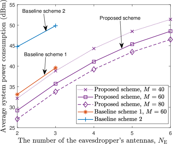
Fig. 4: Average system power consumption versus the number of the eavesdropper’s antennas with γmin=4\gamma^{\min}=4 dB. Baseline schemes 1 and 2 are infeasible in all the channel realizations for NT≤NEN_{\mathrm{T}}\leq N_{\mathrm{E}}, while that for the proposed scheme are feasible.

Fig. 4 demonstrates the average system power consumption versus the number of the eavesdropper’s antennas for cases with a different number of elements at the active IRS. Since there is insufficient DoF and flexibility for optimizing the system resources, baseline schemes 1 and 2 are infeasible in all channel realizations when NE≥NTN_{\mathrm{E}}\geq N_{\mathrm{T}}. In contrast, the proposed scheme admits a feasible solution in the same setting as the former. In particular, as NEN_{\mathrm{E}} increases, the eavesdropper enjoys more spatial DoF for more effective wiretapping. As such, a higher power is allocated to AN at both the BS and the active IRS to neutralize the decoding capability of the eavesdropper and thus the total power consumption increases in the proposed scheme. Furthermore, the average system power consumption can be reduced by increasing the number of active IRS elements. Indeed, the extra spatial DoF offered by the additional IRS elements provides higher flexibility to enhance the signal quality between the BS and the users while effectively mitigating the information leakage to the eavesdropper.

VI Conclusions

We investigated a multi-user MISO downlink communications system with an active IRS in the presence of a multi-antenna eavesdropper. Specifically, both the BS and the active IRS are able to emit the AN for security provisioning. A power minimization design was formulated as a non-convex optimization problem while guaranteeing the secrecy rate between the BS and the users. Our design optimized the precoder and the AN vector at the BS and the amplitude, phase, and mode selection of each active IRS element. A suboptimal solution to the design problem was obtained by applying AO, SCA, and SDR techniques. Simulation results unveiled that the proposed scheme can provide a significant power consumption reduction than the other considered baseline schemes to guarantee the same QoSs. Furthermore, even when the number of eavesdropper antennas exceeds that of the BS, the proposed scheme can still provide secure communication.

According to the Weinstein–Aronszajn identity[16], det⁡(𝐈+𝐀𝐁)=det⁡(𝐈+𝐁𝐀)\mathrm{det}(\mathbf{I}+\mathbf{AB})=\mathrm{det}(\mathbf{I}+\mathbf{BA}), and thus CE,k{C}_{\mathrm{E},k} in constraint C2\mathrm{C2} of 𝒫​1\mathcal{P}1 is equivalent as

log2⁡(det(𝐈NE+𝐐−1​𝐅eq​𝐰k​𝐰kH​𝐅eqH))≤Ckmax\displaystyle\hskip-2.84526pt\log_{2}\Big(\det(\mathbf{I}_{N_{\mathrm{E}}}\hskip-2.84526pt+\hskip-2.84526pt\mathbf{Q}^{-1}\mathbf{F}_{\mathrm{eq}}\mathbf{w}_{k}\mathbf{w}_{k}^{\mathrm{H}}\mathbf{F}_{\mathrm{eq}}^{\mathrm{H}})\Big)\leq C_{k}^{\max}
⇔\displaystyle\Leftrightarrow\,\, log2⁡(1+Tr⁡(𝐰kH​𝐅eqH​𝐐−1​𝐅eq​𝐰k))≤Ckmax\displaystyle\log_{2}\big(1+\hskip-2.84526pt\mathrm{Tr}(\mathbf{w}_{k}^{\mathrm{H}}\mathbf{F}_{\mathrm{eq}}^{\mathrm{H}}\mathbf{Q}^{-1}\mathbf{F}_{\mathrm{eq}}\mathbf{w}_{k})\big)\leq{C_{k}^{\max}}
⇔\displaystyle\Leftrightarrow\,\, 𝐰kH​𝐅eqH​𝐐−1​𝐅eq​𝐰k≤CE,kTol\displaystyle\mathbf{w}_{k}^{\mathrm{H}}\mathbf{F}_{\mathrm{eq}}^{\mathrm{H}}\mathbf{Q}^{-1}\mathbf{F}_{\mathrm{eq}}\mathbf{w}_{k}\leq C_{\mathrm{E},k}^{\mathrm{Tol}}
⇔\displaystyle\Leftrightarrow\,\, Tr⁡(𝐐−1​𝐅eq​𝐰k​𝐰kH​𝐅eqH)≤CE,kTol\displaystyle\mathrm{Tr}(\mathbf{Q}^{-1}\mathbf{F}_{\mathrm{eq}}\mathbf{w}_{k}\mathbf{w}_{k}^{\mathrm{H}}\mathbf{F}_{\mathrm{eq}}^{\mathrm{H}})\leq C_{\mathrm{E},k}^{\mathrm{Tol}}
⇔(a)\displaystyle\stackrel{{\scriptstyle\text{(a)}}}{{\Leftrightarrow}}\,\, λmax​{𝐐−12​𝐅eq​𝐰k​𝐰kH​𝐅eqH​𝐐−12}≤CE,kTol\displaystyle\lambda_{\max}\Big\{\mathbf{Q}^{-\frac{1}{2}}\mathbf{F}_{\mathrm{eq}}\mathbf{w}_{k}\mathbf{w}_{k}^{\mathrm{H}}\mathbf{F}_{\mathrm{eq}}^{\mathrm{H}}\mathbf{Q}^{-\frac{1}{2}}\Big\}\leq C_{\mathrm{E},k}^{\mathrm{Tol}}
⇔\displaystyle\Leftrightarrow\,\, CE,kTol​𝐐−𝐅eq​𝐰k​𝐰kH​𝐅eqH⪰𝟎.\displaystyle C_{\mathrm{E},k}^{\mathrm{Tol}}\mathbf{Q}-\mathbf{F}_{\mathrm{eq}}\mathbf{w}_{k}\mathbf{w}_{k}^{\mathrm{H}}\mathbf{F}_{\mathrm{eq}}^{\mathrm{H}}\succeq\mathbf{0}. (25)

Note that as 𝐐−12​𝐅eq​𝐰k×𝐰kH​𝐅eqH​𝐐−12\mathbf{Q}^{-\frac{1}{2}}\mathbf{F}_{\mathrm{eq}}\mathbf{w}_{k}\times\mathbf{w}_{k}^{\mathrm{H}}\mathbf{F}_{\mathrm{eq}}^{\mathrm{H}}\mathbf{Q}^{-\frac{1}{2}} is a rank one matrix, (a) holds. Then, substitute 𝐐\mathbf{Q} in (8) into (25), the result follows immediately.

References

  • [1] Q. Wu and R. Zhang, “Intelligent reflecting surface enhanced wireless network via joint active and passive beamforming,” IEEE Trans. Wireless Commun., vol. 18, no. 11, pp. 5394–5409, Aug. 2019.
  • [2] Ö. Özdogan, E. Björnson, and E. G. Larsson, “Intelligent reflecting surfaces: Physics, propagation, and pathloss modeling,” IEEE Wireless Commun. Lett., vol. 9, no. 5, pp. 581–585, Dec. 2020.
  • [3] Z. Zhang, L. Dai, X. Chen, C. Liu, F. Yang, R. Schober, and H. V. Poor, “Active RIS vs. passive RIS: Which will prevail in 6G?” arXiv preprint arXiv:2103.15154, 2021.
  • [4] D. Xu, X. Yu, D. W. Kwan Ng, and R. Schober, “Resource allocation for active IRS-assisted multiuser communication systems,” in 2021 55th Asilomar Conf. Signals Syst. Comput., Oct. 2021, pp. 113–119.
  • [5] R. Long, Y.-C. Liang, Y. Pei, and E. G. Larsson, “Active reconfigurable intelligent surface-aided wireless communications,” IEEE Trans. Wireless Commun., vol. 20, no. 8, pp. 4962–4975, Mar. 2021.
  • [6] J. Lončar, A. Grbic, and S. Hrabar, “Ultrathin active polarization-selective metasurface at X-band frequencies,” Physical Review B, vol. 100, no. 7, p. 075131, Oct. 2019.
  • [7] S. Hu, Z. Wei, Y. Cai, C. Liu, D. W. K. Ng, and J. Yuan, “Robust and secure sum-rate maximization for multiuser MISO downlink systems with self-sustainable IRS,” IEEE Trans. Commun., vol. 69, no. 10, pp. 7032–7049, Jul. 2021.
  • [8] Y. Sun, D. W. K. Ng, J. Zhu, and R. Schober, “Robust and secure resource allocation for full-duplex MISO multicarrier NOMA systems,” IEEE Trans. on Commun., vol. 66, no. 9, pp. 4119–4137, Sep. 2018.
  • [9] G. Zhou, C. Pan, H. Ren, K. Wang, and Z. Peng, “Secure wireless communication in RIS-aided MISO system with hardware impairments,” IEEE Wireless Commun. Lett., vol. 10, no. 6, pp. 1309–1313, Mar. 2021.
  • [10] J. Zhang, L. Fu, and X. Wang, “Asymptotic analysis on secrecy capacity in large-scale wireless networks,” IEEE/ACM Trans. Netw., vol. 22, no. 1, pp. 66–79, Feb. 2014.
  • [11] Z. Wang, L. Liu, and S. Cui, “Channel estimation for intelligent reflecting surface assisted multiuser communications: Framework, algorithms, and analysis,” IEEE Trans. Wireless Commun., vol. 19, no. 10, pp. 6607–6620, Jun. 2020.
  • [12] A. Abdipour, G. Moradi, and S. Saboktakin, “Design and implementation of a noise generator,” in Proc. IEEE Int. RF Microw. Conf. IEEE, Dec. 2008, pp. 472–474.
  • [13] J.-F. Bousquet, S. Magierowski, and G. G. Messier, “A 4-GHz active scatterer in 130-nm CMOS for phase sweep amplify-and-forward,” IEEE Tran. on Circuits Syst. I, vol. 59, no. 3, pp. 529–540, Mar. 2011.
  • [14] M. Grant and S. Boyd, “Cvx: Matlab software for disciplined convex programming, version 2.1,” 2014.
  • [15] I. Pólik and T. Terlaky, “Interior point methods for nonlinear optimization,” in Nonlinear optimization. Springer, Jul. 2010, pp. 215–276.
  • [16] J. J. Sylvester, “On the relation between the minor determinants of linearly equivalent quadratic functions,” Lond. Edinb. Dublin philos. mag. j. sci., vol. 1, no. 4, pp. 295–305, 1851.