Dynamics of $2$D fluid in bounded domain via conformal variables

The capillary waves are commonly observed in the ocean swell on the length scale of a few centimeters. They often appear as a result of breaking of steep gravity waves longuet1963generation or other processes related to water wave turbulence, such as the formation of direct energy cascade dyachenko2004weak; korotkevich2008simultaneous. When wind blows on the ocean surface, or a breaking ocean wave is observed, a spray of droplets often is formed when tiny droplets detach from the main body of water.

Leaving aside the ballistic motion induced by gravity, the internal motion of a droplet is dominated by the kinetic energy entrapped in its body, and the surface tension forces acting upon its free surface. The perfect sphere is a minimizer of the surface area of a fluid droplet and hence potential energy due to surface tension attains its minimum value in a spherical droplet. Similarly, in a $2$D fluid the minimal perimeter is attained by a disc-shaped droplet. Once detached from the bulk of the fluid, it carries away angular momentum from the fluid body as a part of its kinetic energy. Both quantities are conserved in time and contribute to its dynamics which can be quite complicated, and is described by the Euler equations with a free boundary. When the angular momentum carried by a droplet is too large to be balanced by surface tension, the droplet may break further into even smaller droplets, and a cascade of multiple breaking droplets observed on a large scale may be contributing to generation of water spray at the crests of steep ocean waves. Some environmental processes, like the gas exchange at the air–water interface, can be greatly enhanced by an effective increase of surface area through droplet generation. It is our aim to understand the internal dynamics of droplets, and the processes that may result in their breaking.

In the present work, we consider nonlinear traveling waves on the free surface of a droplet of radius $R$ induced by a balance of angular momentum and the forces of surface tension. We follow the conformal variables approach originally introduced by Stokes in Stokes1880 and later extended to time-dependent problem in Ovsyannikov1973; Tanveer1991. A framework for studying flows in closed domains (like a fluid blob) as well as on the exterior of an air bubble submerged in a 2D ideal fluid has been developed in Crowdy1999. Our approach is based on the conformal variables technique for bounded domains described in dyachenko2022traveling.

We find families of nonlinear traveling waves that bifurcate from a disc shaped droplet and can be parameterized by an integer number of wavelengths per perimeter of a droplet (the number of lobes, $k$), and the wave steepness. The solutions are found numerically in terms of Fourier series satisfying pseudo–differential nonlinear eigenvalue problem that is qualitatively similar to the Babenko equation for Stokes waves in $2$D babenko1987some and can be solved by similar numerical techniques yang2009newton; Saad2003.

Given wave length $\lambda$, we recover the family of Crapper wave solutions Crapper1957; Longuet1988 in the limit $\lambda\ll R$ ($k\to\infty$). This limit is equivalent to traveling capillary waves in infinite depth fluid. Oscillations of 3D droplets have been a subject of interest since the works of Rayleigh Rayleigh1879, and have been studied both experimentally and analytically, see e.g. Trinh1982. It is yet unclear whether there is a relation between dynamics of $2$D and $3$D droplets.

The text is organized as follows. In the first three sections we describe the motion integrals relevant to droplet mechanics, the conformal variables approach and the equation describing a nonlinear traveling wave (10). Section IV describes the series solution for infinitesimal waves which are employed as the initial guess in the Newton-Conjugate-Residual method yang2009newton; Saad2003 in section V. The main results and conclusions are described in section VII.

We consider the motion of a $2$D ideal fluid in a bounded domain $\mathcal{D}$. The velocity field is given by the gradient of the velocity potential, $\varphi({\bf r},t)$, where ${\bf r}=(x,y)^{T}\in\mathcal{D}$.

The Hamiltonian is the sum of kinetic and potential energy due to the surface tension:

$\displaystyle\mathcal{H}=\frac{1}{2}\iint\limits_{D}\left(\nabla\varphi\right)^{2}\,dxdy+\sigma\int\limits_{\partial D}dl,$

(1)

where $\nabla$ is the $2$D gradient, and $\sigma$ is the surface tension coefficient. The boundary of the fluid domain, $\partial\mathcal{D}$, also known as the free surface, is a time-dependent curve in $2$D.

When the fluid is at rest the shape of the droplet is a perfect disc, a shape that attains the least perimeter given a fixed volume $\mu$; when detached from the body of fluid, droplet carries away angular momentum $\mathcal{J}$ which is conserved:

$\displaystyle\mu=\iint\limits_{D}dxdy\quad\mbox{and}\quad\mathcal{J}=\iint\limits_{D}\left[{\bf r}\times\nabla\varphi\right]\,dxdy.$

(2)

A semi–infinite periodic strip $w=u+iv\in\{-\pi\leq u<\pi,v\leq 0\}$ is conformally mapped to the fluid domain $z=x+iy\in D$ by the complex function $z(w,t)$. The invariant quantities associated with the flow may be expressed in terms of conformal variables as 1$D$ integrals over the free surface $w=u$ ($v=0$); for example, the Hamiltonian becomes

$\displaystyle\mathcal{H}=\frac{1}{2}\iint\limits_{D}\left(\nabla\varphi\right)^{2}\,dxdy+\sigma\int\limits_{\partial D}\,dl=\frac{1}{2}\int\limits_{-\pi}^{\pi}\psi\hat{k}\psi\,du+\sigma\int\limits_{-\pi}^{\pi}|z_{u}|\,du,$

(3)

where $\hat{H}$ is the Hilbert transform, and $\hat{k}=-\hat{H}\partial_{u}$. Here $\psi(u,t)=\varphi(x(u,t),y(u,t),t)$ is the velocity potential at the free surface. The total volume of an incompressible fluid is proportional to the mass of the fluid $\mu$, a trivial constant of motion, and the angular momentum $\mathcal{J}$, given by

		$\displaystyle\mu=\iint\limits_{D}\,dx\,dy=\frac{1}{4i}\int\limits_{-\pi}^{\pi}\left[z\bar{z}_{u}-\bar{z}z_{u}\right]\,du,$		(4)
		$\displaystyle\mathcal{J}=\iint\limits_{D}\left[{\bf r}\times\nabla\phi\right]\,dxdy=-\frac{1}{2}\int\limits_{\partial D}r^{2}\frac{\partial\theta}{\partial{\bf n}}\,dl=-\frac{1}{2}\int\limits_{-\pi}^{\pi}|z|^{2}\psi_{u}\,du,\quad\frac{d\mathcal{J}}{dt}=0,$		(5)

where $r=\sqrt{x^{2}+y^{2}}$ and ${\bf n}$ is the unit normal to the free surface.

The implicit form of complex equations of motion is given by:

		$\displaystyle z_{t}\bar{z}_{u}-\bar{z}_{t}z_{u}=\bar{\Phi}_{u}-\Phi_{u},$		(6)
		$\displaystyle\psi_{t}\bar{z}_{u}-\psi_{u}\bar{z}_{t}+\frac{\Phi_{u}^{2}}{2z_{u}}=i\sigma\partial_{u}\left(\frac{\bar{z}_{u}}{|z_{u}|}\right),$		(7)

where $\Phi=\psi+i\hat{H}\psi$ is the complex potential.

A traveling wave on the free surface of a disc is obtained by seeking conformal map and potential in the form:

$\displaystyle z(u,t)=e^{-i\Omega t}z\left(u-\Omega t\right)\quad\mbox{and}\quad\Phi(u,t)=i\Omega\hat{P}|z|^{2}-\beta t,$

(8)

where $\beta$ is the Bernoulli constant. We note that the equations of motion are invariant under the change of variables $u\to u-\Omega t$, and thus the solution may be sought in the form $z=z(u)$. Substitution of (8) in the equations (6) and (7) leads to an equation for traveling waves:

$\displaystyle 2\beta y_{u}-\frac{\Omega^{2}}{2}\left[x\hat{k}|z|^{2}-\hat{H}\left(y\hat{k}|z|^{2}\right)\right]-\sigma\partial_{u}\left[\frac{x_{u}}{|z_{u}|}-\hat{H}\left(\frac{y_{u}}{|z_{u}|}\right)\right]=0,$

(9)

or, in the complex form,

$\displaystyle 2i\beta z_{u}+\Omega^{2}\hat{P}\left[z\hat{k}|z|^{2}\right]+2\sigma\partial_{u}\hat{P}\left[\frac{z_{u}}{|z_{u}|}\right]=0.$

(10)

For a traveling wave solution, kinematic constants are related via the formula

$\displaystyle\mu\beta=\Omega\mathcal{J}+\frac{\sigma}{2}\langle|z_{u}|\rangle,$

(11)

where angular brackets denote integral over one period, and the last term is the perimeter of the droplet.

Let $w=u+iv\in\mathbb{C}^{-}$, and recall that $e^{-iw}$ is a conformal map from a semi-infinite strip $-\pi<u<\pi$ and $v<0$ to a unit disc. The function $z(u)$ describing the shape of a small amplitude wave is represented by an infinite Fourier series,

$$z(u)=e^{-iu}\left(1+\sum\limits_{k=1}^{\infty}a_{k}e^{-iku}\right),$$

(12)

where $a_{k}$ are the Fourier coefficients. Unless the solution is strongly nonlinear the series is rapidly convergent, and asymptotic solution of the equation (10) can be obtained by a series expansion (12) assuming $|a_{2}|\ll|a_{1}|$.

The first-order approximation is given by

$$z=e^{-iu}\left(1+a_{k}e^{-iku}\right),$$

(13)

where $k\geq 2$ is an integer representing the number of lobes in the solution. When ansatz (13) is plugged into the dynamic condition (7), we find that the Bernoulli constant, $\beta$, and frequency, $\Omega$, must be expanded in series keeping $O(a_{k})$ terms as follows,

$$\beta=\sigma+O(a_{k}^{2}),\quad\Omega^{2}=\frac{(k^{2}-1)\sigma}{k}+O(a_{k}^{2}).$$

(14)

The dispersion relation of linear waves $\Omega(k)$ was also obtained in Ref. dyachenko2022traveling.

The second order approximation to the solutions of (10) can be found by keeping the first two terms in the Fourier expansion (12). We will consider the case of $k=2$, but generalization to arbitrary number of lobes $k$ can be done analogously. We now seek solution in the form:

$$z=e^{-iu}\left(1+a_{2}e^{-2iu}+a_{4}e^{-4iu}\right),$$

(15)

and substitute it into the equation (10) for traveling waves to match the corresponding terms in the expansion. We expand the equation (10) in Fourier series and require that the first three series’ coefficients vanish, which results in the following expressions:

		$\displaystyle e^{-iu}\left[2(\beta-\sigma)+\frac{1}{128}\bigl(64(9\sigma+4\Omega^{2})a_{2}^{2}\bigr)+O(a_{2}^{4})\right]$		(determines $\beta$)
		$\displaystyle+e^{-3iu}a_{2}\left[(6\beta-9\sigma+2\Omega^{2})+\left(\frac{9}{8}(-9a_{2}^{2}+20a_{4})\sigma+4a_{4}\Omega^{2}\right)+O(a_{2}^{4})\right]$		(determines $\Omega^{2}$)
		$\displaystyle+e^{-5iu}\left[128\bigl(5(8a_{4}\beta+9a_{2}^{2}\sigma-20a_{4}\sigma)+8(a_{2}^{2}+2a_{4})\Omega^{2}\bigr)+O(a_{2}^{4})\right],$		(determines $a_{4}$)

thus the second order approximation for the Bernoulli constant $\beta$ and frequency $\Omega$ are determined by

$\displaystyle\beta=\sigma\left(1-\frac{15}{4}a_{2}^{2}\right)+O(a_{2}^{4}),\quad\Omega^{2}=\sigma\left(\frac{3}{2}-\frac{25}{4}a_{2}^{2}\right)+O(a_{2}^{4}),$

and $a_{4}=\frac{19}{12}a_{2}^{2}$. The first and second order approximations are used to provide the initial guess for the Newton’s method applied to the fully nonlinear equation (10). The discussion of fully nonlinear solutions and implementation of Newton’s method is presented in the following sections.

In a more general case, $k\geq 2$, the second order approximation is found analogously:

$$z=e^{-iu}(1+a_{k}e^{-iku}+a_{2k}e^{-2iku})+O(a_{k}^{3}),$$

(16)

and by repeating the same steps to keep orders up to $O(a_{k}^{2})$, we obtain

	$\displaystyle\beta$	$\displaystyle=\left(1-\frac{a_{k}^{2}}{4}(k+1)(3k-1)\right)\sigma+O(a_{k}^{4}),$		(17a)
	$\displaystyle\Omega^{2}$	$\displaystyle=\frac{k^{2}-1}{4k(1+2k^{2})}\left(4+8k^{2}+a_{k}^{2}(1+k)(6-k(22+k+k^{2}))\right)\sigma+O(a_{k}^{4}),$		(17b)
	$\displaystyle a_{2k}$	$\displaystyle=\frac{(1+k)((7+2k)k-3)}{4(1+2k^{2})}a_{k}^{2}+O(a_{k}^{4}).$		(17c)

Conformal map (16) with parameters (17) can serve as an initial guess for numerical iterative procedure such as Newton’s method.

The nonlinear solutions of (10) are found by applying Newton iterations. Given an initial guess, $z^{(0)}(u)$, or an approximation, $z^{(m)}$ at an iteration $m$, we may write the exact solution of (10) as follows,

$$z=z^{(m)}+\delta z,$$

(18)

where $z$ is the unknown exact solution of (10), $m\geq 0$ is the iteration number, and $\delta z$ is the correction term to be determined. The formula (18) is substituted into the equation (10) assuming $||\delta z||\ll||z^{(m)}||$ and only the linear terms in $\delta z$ are kept:

	$\displaystyle 2i\beta\delta z_{u}+\Omega^{2}\hat{P}\left[\delta z\hat{k}\left|z^{(m)}\right|^{2}+z^{(m)}\hat{k}\left(z^{(m)}\delta\bar{z}+\bar{z}^{(m)}\delta z\right)\right]\qquad\,\quad$
	$\displaystyle+\sigma\partial_{u}\hat{P}\left[\frac{z^{(m)}_{u}}{\left|z^{(m)}_{u}\right|^{3}}\left(\bar{z}_{u}^{(m)}\delta z_{u}-z^{(m)}_{u}\delta\bar{z}_{u}\right)\right]+\hat{N}(z^{(m)})=0,$

where $N(z)$ is defined as follows:

$\displaystyle\hat{N}(z):=2i\beta z_{u}+\Omega^{2}\hat{P}\left[z\hat{k}|z|^{2}\right]+2\sigma\partial_{u}\hat{P}\left[\frac{z_{u}}{|z_{u}|}\right],$

(19)

which is exactly the left-hand side of the equation (10). It is often more convenient to implement iterations for a real unknown function, and we may recall that the components of the conformal map are not independent and are related via the Hilbert transform, i.e. since $z=x+iy$ and $\delta z=\delta x+i\delta y$, then

$\displaystyle x=-\hat{H}y,\quad\delta x=-\hat{H}\left[\delta y\right],$

and the linearized equation (V) is equivalent to an auxiliary real equation for one real unknown function $\delta y$ given by

		$\displaystyle-2\beta\delta y_{u}+\Omega^{2}\left(-\frac{1}{2}(\hat{\mathcal{H}}\delta y)\hat{k}|z|^{2}-(\hat{\mathcal{H}}y)\hat{k}((\hat{\mathcal{H}}y)(\hat{\mathcal{H}}\delta y)+y\delta y)-\hat{\mathcal{H}}\left[\frac{1}{2}\delta y\hat{k}|z|^{2}+y\hat{k}((\hat{\mathcal{H}}y)(\hat{\mathcal{H}}\delta y)+y\delta y)\right]\right)$
		$\displaystyle\hskip 18.49988pt+\sigma\partial_{u}\left(-\frac{y_{u}}{|z_{u}|^{3}}(-(\hat{\mathcal{H}}y)_{u}\delta y_{u}+y_{u}(\hat{\mathcal{H}}\delta y)_{u})-\hat{\mathcal{H}}\left[-\frac{(\hat{\mathcal{H}}y)_{u}}{|z_{u}|^{3}}((\hat{\mathcal{H}}y)_{u}\delta y_{u}-y_{u}(\hat{\mathcal{H}}\delta y)_{u})\right]\right)$
		$\displaystyle\hskip 18.49988pt-2\beta y_{u}+\frac{1}{2}\Omega^{2}\left(-(\hat{\mathcal{H}}y)\hat{k}|z|^{2}-\hat{\mathcal{H}}\left[y\hat{k}|z|^{2}\right]\right)+\sigma\partial_{u}\left(\frac{-(\hat{\mathcal{H}}y)_{u}}{|z_{u}|}-\hat{\mathcal{H}}\left[\frac{y_{u}}{|z_{u}|}\right]\right)=0,$

or, writing it in compact form,

$$L_{1}(y,\delta y)+L_{0}(y)=0.$$

(20)

When Hilbert transform is applied to the equation (20), we obtain the linear equation for $\delta y$:

$$\hat{H}L_{1}(y,\delta y)\delta y=-\hat{H}L_{0}(y)$$

(21)

with a self-adjoint operator with respect to the standard inner product:

$$(f,g)=\int\limits_{-\pi}^{\pi}f(x)g(x)dx$$

(22)

for real-valued $f(x)$ and $g(x)$. A linear system with a self-adjoint operator is amenable to be solved by the Conjugate-Residual (CR) method. We solve (20) numerically using a Fourier pseudospectral method to approximate the function $z$. The projection operator $\hat{\mathcal{P}}$, Hilbert transform $\hat{H}$ and derivatives with respect to $u$ are applied as Fourier multipliers. At each Newton iteration a new linear system is solved with CR, and Newton iterations are performed until a required tolerance, $\varepsilon$, is attained: $\|\hat{N}\left(z^{(m)}\right)\|\leq\varepsilon$.

The second order approximation (15) is used as an initial guess, $z^{(0)}$, to initiate the Newton’s iterations. Once a nonlinear solution is determined with a given set of parameters, it is used to follow the solution branch to strongly nonlinear waves by parameter continuation, either in $\beta$ or $\Omega^{2}$, while keeping surface tension $\sigma$ fixed.

A constraint relating the physically relevant quantities,

$$\mu\beta-4\Omega J-2\sigma L=0,$$

(23)

is used to determine the value of $\Omega^{2}$ if $\beta$ is known, or vice versa. Here $4i\mu=\int_{-\pi}^{\pi}(z\bar{z}_{u}-\bar{z}z_{u})\,du$ is the droplet area, $L=\int_{-\pi}^{\pi}|z_{u}|du$ is the droplet perimeter length, and $4J=-\Omega\int_{-\pi}^{\pi}|z|^{2}\hat{k}|z|^{2}du$ is the rescaled angular momentum.

The solutions of (10) enjoy two symmetries, one is related to the freedom of choosing the phase shift in the rotation angle, and the second symmetry is related to rescaling of the droplet surface. The choice of phase shift is fixed by seeking only even $y(u)$, and in order to hold the droplet area $\mu$ fixed, we rescale $z(u)$, $\beta$, $L$ and $J$ once a solution of (10) is obtained,

$$z(u)\rightarrow\frac{z}{\nu},\quad\mu\rightarrow\frac{\mu}{\nu^{2}},\quad L\rightarrow\frac{L}{\nu},\quad J\rightarrow\frac{J}{\nu^{4}}.$$

(24)

For example, choosing $\nu=\sqrt{\mu/\pi}$ ensures that $\mu=\pi$ is preserved. The number of Fourier modes that we considered is limited by $N=65536$, and the magnitude of the Fourier mode at series truncation is $10^{-9}$. The relative tolerance for solving the linear system (20) in the CR method is $10^{-2}$, and the nonlinear residual for Newton’s iterations $\varepsilon=10^{-9}$.

The nonlinear waves obtained with Newton-Conjugate-Residual method are illustrated in Fig. 3 with $k=4$ and $k=25$ lobes. In addition, we show parameter curves $\Omega^{2}$ vs $H/\lambda$ (see Fig. 4, left) and $\mathcal{J}$ vs $H/\lambda$ (see Fig. 4, right). Here $H$ denotes the height of the wave, and $\lambda$ is the spatial period.

We illustrate two typical solutions of the nonlinear equation (10) by showing the shape of the free surface and the velocity field in Fig. 1. We find that a traveling wave becomes elongated as the steepness grows, and the number of Fourier modes necessary to resolve the solution grows with wave steepness (see Fig. 2), indicating the existence of a singularity in the analytic continuation of $z(w)$ to the upper half-plane $w\in\mathbb{C}^{+}$. The nature of this singularity, and the existence of a limiting wave is the subject of ongoing research.

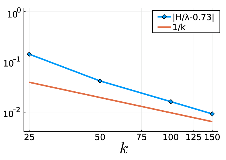
The numerical simulations and theoretical considerations suggest that a solution with sufficiently many lobes approaches the Crapper wave as the number of lobes grows (Fig. 3). The right panel of Fig. 3 indicates that steepness of the self-touching (limiting) Crapper wave is approached by the nonlinear solutions of (10) as the number of lobes $k$ increases. This can be explained as follows: the wavelength is given by $\lambda=2\pi/k$, and as it becomes small compared to the perimeter of the droplet (when $k$ grows), the effects of local curvature become less significant and vanish in the limit $k\to\infty$. Another open question concerns the number of lobes for which self-touching of neighboring waves occurs (Crapper scenario) versus the presently unknown limiting scenario for few lobes, e.g. $k=2$ and $k=3$ for which no indication of a tendency to self-intersect was observed.

Breaking of water waves in deep ocean is associated with generation of water droplet spray. The latter partially accounts for the energy–momentum transfer in wave turbulence. The physical processes that generate water spray have been observed in physical ocean ErininEtAlSprayGeneration2019, as well as theoretically DyachenkoNewell2016. As plunging breaker develops on the crest of an ocean wave, there is an abrupt growth of small scale features, and several physical mechanisms suddenly come into play. The force of the surface tension, normally having little effect on long gravity waves becomes one of the dominant forces at the crest of a breaking wave. The detachment of a water droplet from a plunging breaker is a complicated and nonlinear process, and the present work does not make an attempt to understand it to the full extent.

We considered a problem of deformation of a fluid disc with a free boundary subject to the force of surface tension. We found that a conformal map associated with such a flow satisfies a pseudo–differential equation that is similar to Babenko equation for the Stokes wave. We demonstrate the results of numerical simulation with initial data close to linear waves, and observe excellent agreement for small amplitude waves, and report significant deviations as amplitude grows.

The nonlinear equation (9), or its complex form (10), are solved by the Newton-Conjugate-Residual method yang2009newton; Saad2003 that is also applicable to the Stokes wave problem. The present work is a precursor to further investigation of nonlinear waves, and of particular interest are the questions of existence of the limiting wave, its nature and singularities. One may speculate that the limiting wave will not form an angle on the surface, since it would make the potential energy grow; yet the numerical simulations suggest the breaking of a droplet (for small number of lobes), and a tendency to develop a self-touching solution like the Crapper wave (for large number of lobes). The study of limiting scenarios is the subject of ongoing work.

References

- (1) K. I. Babenko, Some remarks on the theory of surface waves of finite amplitude, in Doklady Akademii Nauk, vol. 294, Russian Academy of Sciences, 1987, pp. 1033–1037.
- (2) G. Crapper, An exact solution for progressive capillary waves of arbitrary amplitude, Journal of Fluid Mechanics, 2 (1957), pp. 532–540.
- (3) D. Crowdy, Circulation-induced shape deformations of drops and bubbles: exact two-dimensional models, Physics of Fluids, 11 (1999), pp. 2836–2845.
- (4) A. I. Dyachenko, A. O. Korotkevich, and V. E. Zakharov, Weak turbulent kolmogorov spectrum for surface gravity waves, Physical review letters, 92 (2004), p. 134501.
- (5) S. Dyachenko and A. Newell, Whitecapping, Studies in Applied Mathematics, 137 (2016), pp. 199–213.
- (6) S. A. Dyachenko, Traveling capillary waves on the boundary of a fluid disc, Studies in Applied Mathematics, 148 (2022), pp. 125–140.
- (7) M. Erinin, S. Wang, R. Liu, D. Towle, X. Liu, and J. Duncan, Spray generation by a plunging breaker, Geophysical Research Letters, 46 (2019), pp. 8244–8251.
- (8) A. O. Korotkevich, Simultaneous numerical simulation of direct and inverse cascades in wave turbulence, Physical review letters, 101 (2008), p. 074504.
- (9) M. Longuet-Higgins, The generation of capillary waves by steep gravity waves, Journal of Fluid Mechanics, 16 (1963), pp. 138–159.
- (10) M. Longuet-Higgins, Limiting forms for capillary-gravity waves, Journal of Fluid Mechanics, 194 (1988), pp. 351–375.
- (11) L. Ovsyannikov, Dynamika sploshnoi sredy, lavrentiev institute of hydrodynamics, Sib. Branch Acad. Sci. USSR, 15 (1973), p. 104.
- (12) L. Rayleigh et al., On the capillary phenomena of jets, Proc. R. Soc. London, 29 (1879), pp. 71–97.
- (13) Y. Saad, Iterative methods for sparse linear systems, SIAM, 2003.
- (14) G. Stokes, On the theory of oscillatory waves, Trans. Camb. Phil. Soc., 8 (1847), pp. 411–455.
- (15) S. Tanveer, Singularities in water waves and rayleigh–taylor instability, Proceedings of the Royal Society of London. Series A: Mathematical and Physical Sciences, 435 (1991), pp. 137–158.
- (16) E. Trinh and T. Wang, Large-amplitude free and driven drop-shape oscillations: experimental observations, Journal of Fluid Mechanics, 122 (1982), pp. 315–338.
- (17) J. Yang, Newton-conjugate-gradient methods for solitary wave computations, Journal of Computational Physics, 228 (2009), pp. 7007–7024.