Radio Spectral Energy Distributions for Single Massive Star Winds with Free-Free and Synchrotron Emission
Abstract
The mass-loss rates from single massive stars are high enough to form radio photospheres at large distances from the stellar surface where the wind is optically thick to (thermal) free-free opacity. Here we calculate the far-infrared, millimeter, and radio band spectral energy distributions (SEDs) that can result from the combination of free-free processes and synchrotron emission, to explore the conditions for non-thermal SEDs. Simplifying assumptions are adopted in terms of scaling relations for the magnetic field strength and the spatial distribution of relativistic electrons. The wind is assumed to be spherically symmetric, and we consider the effect of Razin suppression on the synchrotron emission. Under these conditions, long-wavelength SEDs with synchrotron emission can be either more steep or more shallow than the canonical asymptotic power-law SED from a non-magnetic wind. When non-thermal emission is present, the resultant SED shape is generally not a power-law; however, the variation in slope can change slowly with wavelength. Consequently, over a limited range of wavelengths, the SED can masquerade as approximately a power law. While most observed non-thermal long-wavelength spectra are associated with binarity, synchroton emission can have only a mild influence on single-star SEDs, requiring finer levels of wavelength sampling for detection of the effect.
Keywords:
radiation mechanisms: nonthermal — stars: early-type — stars: magnetic fields — stars: mass loss — stars: winds, outflows — radio continuum: starsI Introduction
Massive stars are an important part of the story of cosmic evolution (Bromm & Larson 2004; Heger & Woosley 2010; Madau & Dickinson 2014, e.g.,) due to their luminous but short lifetimes (Langer 2012, e.g.,), their explosive endings (Woosley et al. 2002, e.g.,), the extreme remnants that they produce (Heger et al. 2003, e.g.,), and their strong influence on galactic evolution (Hopkins et al. 2012, e.g.,). Our developing understanding of massive star evolution is informed by factors such as stellar rotation, magnetism, and mass-loss rates. Ongoing observational and theoretical investigations continue to refine our ability to measure and interpret these properties for massive stars.
Radio studies are a foundational approach for determining the relatively high mass-loss rates () from massive stars, which can be large enough to produce radio photospheres that form in the stellar wind (Panagia & Felli 1975; Wright & Barlow 1975; Abbott et al. 1980; Abbott et al. 1981; Abbott et al. 1986; Bieging et al. 1989; Leitherer et al. 1995; Leitherer et al. 1997). The radio flux () is typically attributed to thermal (free-free) emission, and is proportional to both the mass-loss rate of the star and the terminal velocity of the wind () via (Lamers & Cassinelli 1996). However, additional factors such as globally structured magnetic fields (Owocki & ud-Doula 2004; Daley-Yates et al. 2019, e.g.,), non-thermal emission from gyrosynchrotron processes (White 1985; Chen & White 1994; Van Loo et al. 2006, e.g.,), and the existence of structured wind flows (Blomme & Runacres 1997; Nugis et al. 1998; Fullerton et al. 2006; Puls et al. 2006; Ignace 2016, “clumping”; e.g.,), have presented challenges for how radio measures can be used to infer values. An improved understanding of how these processes affect the shape of the spectral energy distribution (SED), and thus interpretations of the stellar mass-loss rate, is therefore required.
The discussion of non-thermal radio emission from massive stars has often focused on synchrotron emission in massive colliding wind binaries (Williams et al. 1994; Pittard et al. 2006; Falceta-Gonçalves & Abraham 2012; Parkin et al. 2014; Benaglia et al. 2015; De Becker et al. 2017, CWB; e.g.,). Electrons are accelerated at the shocks formed from the collision of highly supersonic wind flows, and the in situ magnetism where synchrotron emission is generated derives from a stellar magnetic field. A tremendous advantage of a CWB system is the opportunity to observe cyclical variations in the non-thermal spectrum. This variability provides diagnostic leverage to produce globally self-consistent models for the wind properties, shock properties, magnetism, and the physics underlying particle acceleration (Blomme et al. 2017; De Becker 2018, e.g.,).
Although CWB systems have considerable potential to describe the non-thermal emission from massive star binaries, they cannot be used to fully characterize the non-thermal emission from (purportedly) single early-type stars. In recent years, an increasing number of these have been detected, in no small part due to the successes of the spectropolarimetric surveys that have provided direct measurements of large-scale, nearly dipoler11 1 The assumption of a (nearly) dipolar magnetic topology is generally appropriate (Donati & Landstreet 2009, e.g.,). However, there are some notable exceptions, including Sco (Donati et al. 2006, HD 149438, B0.2 V;), HD 37776 (Kochukhov et al. 2011, B2V;), and CVn (Silvester et al. 2014, B9p;), which have fields with significantly more complex magnetic topologies. surface magnetic fields in massive stars (Alecian et al. 2014; Fossati et al. 2015; Morel et al. 2015; Wade et al. 2016; Grunhut et al. 2017, e.g., MiMeS, BOB;). The magnetic fields of O- and B-type stars channel the stellar wind into a structurally complex magnetosphere, which can provide the conditions necessary for synchrotron emission (Trigilio et al. 2004; Leto et al. 2006; Leto et al. 2021; Shultz et al. 2022, e.g.,). Non-thermal radio spectra of single, magnetic massive stars have been observed in several instances (Kurapati et al. 2017; Leto et al. 2017; Leto et al. 2018, e.g.,).
White 1985 published a seminal paper exploring the modeling and application of radio synchrotron emission for massive star winds. The work was later expanded by Chen & White 1991; White & Chen 1992; Chen & White 1994; White & Chen 1994, both in terms of including additional physical processes (e.g., inverse Compton cooling), and for consideration of very high-energy emissions. Two developments emerged from this series. First, it appeared that the majority of sources displaying non-thermal radio emission were in binaries, hence the increased focus on modeling of colliding wind binary systems (Dougherty et al. 2003; Pittard et al. 2021, e.g.,). Second was the recognition that there are challenges for understanding how relativistic electrons can survive and/or be energized at large radii in the wind (Van Loo et al. 2004; Van Loo et al. 2005; Van Loo et al. 2006). While these challenges remain, non-thermal radio emission has been observed in a few non-magnetic, purportedly single, early-type stars (Dougherty & Williams 2000, e.g.,). There is thus a need to further develop the theoretical description of how free-free and non-thermal emission jointly affect the SED, in order to provide benchmarks for these data.
In this paper, we present several new models of far-infrared, millimeter, and radio band spectral energy distributions (SEDs) resulting from the combination of thermal (free-free) and non-thermal (synchrotron) emissions. Section II develops the model components. In particular, our goal is to examine general trends for single-star winds, and to this end, we consider spherical winds and adopt scaling relations for the magnetic field strength and the density of high-energy electrons. Section III reports the results of our analysis. Finally, in Section IV, we discuss these results in light of the current data and interpretation of radio SEDs for massive-star winds.
II Modeling Radio SEDs
II.1 Thermal Free-Free Emission
Our model is based on a smooth, spherically symmetric wind. While it is clear that magnetism can alter the wind density and vector flow from a spherical geometry, a spherical wind is appropriate for a qualitative exploration of how synchrotron emission can influence radio SED shapes. Additionally, unlike numerically intensive MHD simulations and detailed radiative transfer, semi-analytic approaches afforded by simplifying assumptions (such as a spherical wind density) allows for a rapid exploration of the parameter space.
The emission coefficient for thermal free-free processes, expressed in terms of the power per unit frequency per unit volume per steradian, is written as (Rybicki & Lightman 1986, e.g.,)
| (1) |
where is the root-mean-square charge of the ion, is the gas temperature, and are respectively the free electron and ion densities, is the observation frequency, and is the free-free Gaunt factor (Brussaard & van de Hulst 1962; Hummer 1988, e.g.,). In the exponential, and are the usual Planck and Boltzmann constants. The numerical constant has been evaluated in cgs units.
In the Rayleigh-Jeans limit appropriate at long wavelengths where , the expression for the emission coefficient becomes
| (2) |
where we have scaled the temperature and ion number densities by fiducial values similar to those found in massive star winds.
The absorption coefficient, written here as the product of the opacity coefficient and the mass density, is given by (Rybicki & Lightman 1986, e.g.,)
| (3) |
which in the Rayleigh-Jeans limit is approximated as
| (4) |
Note that we now express the absorption coefficient in terms of the observation wavelength . The source function for free-free radiation is therefore
| (5) | |||||
We can estimate the extent of the radial photosphere (Cassinelli & Hartmann 1977) assuming the wind is optically thick to the free-free opacity (eq. [4]), with speed . The optical depth of a location in the wind is given by the integral of the free-free opacity along the observer’s line-of-sight,
| (6) |
where , is the impact parameter for a ray through the wind, and gives the angle between the radial direction and the observer’s line-of-sight.
We introduce as the radius at which an optical depth of unity is achieved, defined through
| (7) |
For an isothermal wind with K, setting , along with , the effective radius , expressed in terms of the stellar radius , is
| (8) |
Here, we scale the wavelength by a fiducial value of , and the stellar radius by . The number density scale constant ,
| (9) |
is derived from mass continuity (assuming spherical symmetry), where is the mass-loss rate, is the terminal velocity of the wind, and is the mean molecular weight per free electron. With , a wind of entirely ionized hydrogen would have , whereas a wind of entirely singly-ionized helium would have .
Equation (8) shows that the extent of the radio photosphere increases with wavelength, albeit the increase is more shallow than that from a linear dependence on . The radio photosphere at , assuming cm-3, is extensive22 2 A wind density scale of cm-3 is applicable to WR stars, which have a very dense wind environment. For OB supergiants, a wind density scale of cm-3 would be more appropriate. See also Appendix C.; however, ion abundances, the temperature and ionization state of the gas, and the stellar radius will realistically alter the value of , even assuming that does not change. Furthermore, the presence of clumping (Lucy & White 1980; Owocki et al. 1988, structured wind flows believed to result from the intrinsic instabilities associated with the wind-driving physics, see e.g.,) in the wind would also extend the radio photosphere (Ignace 2016).
Radio SEDs purely from free-free opacity have been well-studied. Wright & Barlow 1975 and Panagia & Felli 1975 derived the canonical SED power-law result, with the radio flux for a spherical wind, at long () wavelengths for which the extent of the radio photosphere is much greater than the stellar radius. Schmid-Burgk 1982 found that under the assumption of power-law distributions for the wind density and temperature, axisymmetric winds have SED slopes with the same power-law dependence of the frequency () as from spherically symmetric winds (although the luminosity level is different from the spherical result). This highlighted the idea that the SED slope is governed by the isophotal growth rate as a function of wavelength. Power-law SEDs result for isophotes whose shapes are invariant with wavelength. Ultimately, the expanding radio photosphere with wavelength provides an opportunity for mapping the wind density and geometry as a function of wavelength. For example, the canonical result of , while not unique, can generally be taken as evidence of a spherically symmetric wind expanding at a constant speed.
Free-free radio SEDs have been evaluated for a variety of additional considerations. A change in the SED power-law slope can result from a change in the geometry of the circumstellar medium. The study of Be stars performed by Klement et al. 2017 provides a useful example. The authors found that disk truncation can lead to a SED slope that steepens toward , which is suggestive of an as-yet-undetected binary companion. The influence of clumping for free-free radio SEDs has also been considered (Abbott et al. 1981; Blomme & Runacres 1997; Ignace et al. 2003; Ignace 2016, e.g.,). Clumping affects the opacity, impacting the location of the effective radius . Clumping also increases the emissivity, which scales as the square of density. The end result is that mass-loss rates derived from radio luminosities will be overestimated if clumping is not taken into account.
II.2 Synchrotron Emission
For a single electron, the specific luminosity of synchrotron emission is (Rybicki & Lightman 1986; Dougherty et al. 2003)
| (10) |
where is the magnetic field strength, is the electron mass, is the electron charge, is the pitch angle, and gives the spectral slope as a function of frequency. The quantity is the cut-off frequency, given by
| (11) |
where is the Lorentz factor of the relativistic electrons. For an electron, , or in terms of wavelength, .
The synchrotron spectrum can be derived from a power-law distribution of free electrons. At a given location in the wind, the energy distribution of the electron number density can be represented as
| (12) |
where is the energy, is a scale constant, and is the power-law exponent for the distribution. This can be recast in terms of the Lorentz factor for the relativistic electrons, with
| (13) |
where is the corresponding scale constant. Note that with respect to units, number density, but has units of energy that depend on the value of . The ratio of the scale constants is thus
| (14) |
The value of the scale constants and can vary with pitch angle (Rybicki & Lightman 1986), but we ignore such pitch angle effects for this study.
The number density of relativistic electrons associated with the production of synchrotron emission is then
| (15) |
The power-law index can vary with radius (Van Loo et al. 2005, e.g.,), but we choose33 3 Other values could certainly be used: Van Loo et al. 2004 suggest a steeper value with between 2 and 3. We adopt here the choice of to facilitate our quantitative examples. a constant value of , which is commonly adopted for strong shocks (see Ellison & Eichler 1985; Eichler & Usov 1993, and sources therein).
If we assume and for all locations in the wind, the number density of relativistic electrons becomes
| (16) |
where is a power-law exponent that is a free parameter of our model. The case of corresponds to an inverse-square decline of density of high-energy elections , matching the scaling of the gas density with radius in the asymptotic constant expansion portion of the wind.
Simplifying for the specific case of , we find that . Assuming equipartition, the scale constant for the particle distribution is expressed as (Dougherty et al. 2003)
| (17) |
where is the energy density of the relativistic particles, and is the largest value of achieved by any particle.
The emission coefficient for synchrotron processes, expressed as power per unit frequency per unit volume per steradian, is (Rybicki & Lightman 1986)
| (18) | |||||
where we choose for the pitch angle.
The absorption coefficient for synchrotron processes is given by (Rybicki & Lightman 1986)
| (19) | |||||
The source function for the synchrotron emission is then
| (20) | |||||
| (21) |
where
| (22) |
with
| (23) | |||||
| (24) | |||||
| (25) | |||||
| (26) |
Using and equation (14), the expressions for the synchrotron emission coefficient, opacity, and source function reduce to
| (27) | ||||
| (28) | ||||
| (29) |
It is possible to develop an “effective photosphere” analysis for pure, optically thick synchrotron radiation, following the approach of Cassinelli & Hartmann 1977. Details on the full solution and the approximation of an effective photosphere are given in Appendix A. With equation (16), and a field strength that declines like a toroid44 4 With flux freezing for highly ionized winds, rotation generally leads to a toroidal field topology (Ignace et al. 1998, e.g., ). with
| (30) |
where the “” notation indicates a value at the base of the stellar wind, the extent of the radio photosphere will then scale as . The corresponding specific radio luminosity becomes . For a choice of in , the photospheric radius will grow as , close to the value for free-free emission. However, the SED slope is somewhat steeper than the case of free-free, with . We note that for large values of , the radius of the synchrotron radio photosphere approaches a constant with wavelength, and the SED steepens to . However, there are other factors that influence the SED, such as Razin suppression, addressed below.
II.3 The Razin Effect
The Razin effect (Dougherty et al. 2003, e.g.,) refers to the suppression of synchrotron emission due to the refractive index of the plasma. It is dependent on the plasma frequency, and the frequency at which the effect becomes important is given by (Van Loo et al. 2004, e.g.,):
| (31) |
The suppression of the synchrotron emission scales as , where . At frequencies lower than (or wavelengths longer than ), the synchrotron emission is strongly reduced.
It is useful to develop a scale of where in the wind the Razin effect becomes significant. To provide an estimate, we assume the electron density decreases as , and the field strength decreases as . With a wind density of cm-3, and a stellar field strength of G, equation (31) gives cm at a radius of . At larger radii, the Razin wavelength will be greater. Consequently, for an observation wavelength of 1 cm, the Razin effect will suppress synchrotron emission for , but not for .
III SEDs from Winds with Free-Free and Synchrotron Emission
| 0.0, 0.5, 1.0 | |
| 1 | |
| 100 | |
| 30,000 | |
| 0 (no Razin), | |
| 1, 3, 9, 27, 81 |

We now consider an ionized and magnetized wind that is spherically symmetric, with both free-free and synchrotron opacities. The source function is
| (32) |
Except for very long wavelengths or very large distances in the wind, it is reasonable to expect that the synchrotron opacity is considerably smaller than the free-free opacity (Appendix A), so that the source function reduces to
| (33) |
with the free-free opacity (eq. [4]) as the sole contributor to the absorption coefficient.
From equation (6), the optical depth of the thermal absorption is the line-of-sight integral of the free-free opacity, along a constant impact parameter. The expression is analytic, and integrates to
| (34) |
where , , and . The angle varies over a range of [0, ], with describing the hemisphere of the observer. For simplicity we have defined the constant
| (35) |
With these quantities, and ignoring any radio emission from the star itself, the formal solution for a radio SED from an isothermal wind, is
| (36) | |||||
where , and we have ignored any contribution from the stellar disk. Note that we ignore Razin suppression of the synchrotron emission in this expression, which will be discussed below.
The first integral in equation 36 can be evaluated analytically as
| (37) | |||||
where in the second equality we have used
| (38) | |||||
with . Using the appropriate approximation for in the Rayleigh-Jeans limit, this expression can be recast as
| (39) |
with
| (40) |
as the scaling for the specific luminosity, with units of erg s-1 Hz-1. For the sake of illustrative models, we ignore the wavelength dependence of the free-free factor and set , yielding . Inclusion of would produce the canonical result.
The second integral in equation (36) can be recast as
| (41) |
where we have applied equation (27), assuming , and the constant .
For the case of , for an optically thick wind (), equation (41) can be solved analytically to express the wavelength dependence of the SED,
| (42) | |||||
where
| (43) |
and the constant is equal to
| (44) | |||||
Here, we have applied a fiducial scaling for the surface magnetic field . We note that is dependent on a number of parameters, especially considering that (eq. [9]) also depends on the stellar , , and . Thus a given may apply to a wide combination of observables. Table 1 lists the values of considered for our model SEDs.
The formal solution is then
| (45) |
While this result is essentially unphysical, since at sufficiently long wavelengths the luminosity integrated over wavelength is unbounded, (45) is useful for illustrating the transition of the SED from a thermal to a non-thermal spectrum. Model SEDs without the Razin suppression of the synchrotron emission (i.e., ) are shown as the red curves in Figure 1. These models show that the radio spectrum follows the curve expected from thermal emission at short wavelengths, but then becomes modified by the synchrotron emission at long wavelengths.
Including the Razin effect (suppressing synchrotron emission) in the formal solution yields
| (46) | |||||
where is the Razin wavelength (eqs. [30] and [31]). The Razin wavelength scale constant is defined as
| (47) |
Figure 1 also shows model SEDs that include the Razin effect (black curves). The inclusion of Razin suppression significantly diminishes the synchrotron component at long wavelengths.
IV Discussion
The synthetic SEDs shown in Figure 1 indicate that the inclusion of synchrotron emission can have a significant impact on the shape of the long-wavelength SED, even when Razin suppression is considered. In this regime, the SED is no longer dominated by thermal free-free emission, and so deviates from the canonical power law slope. This change is most pronounced when there is a fixed, constant ratio between the wind density and number density of relativistic electrons (left column).
For steeper distributions of relativistic electrons, the wavelength at which the free-free emission ceases to dominate the SED decreases. Razin suppression of the synchrotron emission becomes more pronounced, producing an SED with a slope that closely resembles the thermal power-law result. This implies that a sufficiently steep distribution of relativistic electrons may produce an SED with a power-law slope that mimics the result for thermal emission, particularly in a given waveband.
Our results indicate that, in the absence of other factors, synchrotron emission can influence single-star SEDs, although a relatively fine degree of wavelength sampling may be needed for detection of the effect owing to the gradual change in SED slope. Although we do not directly consider magnetic massive stars as a part of this analysis, we briefly explore the effect of a latitudinally dependant toroidal field on the shape of the SED in Appendix B.
The models reported here explore different distributions for the population of relativistic electrons using a power-law prescription for , although we offer no model for either how or where electrons are accelerated or transported throughout the wind. Indeed, the processes through which non-thermal synchrotron emission is produced in single, massive stars are still unclear. For stars with sufficient mass-loss rates to produce radio excesses in the wind, but with only modest surface magnetic fields (well below 1 kG), the radio photospheres is relatively extended compared to where synchrotron emission would typically form in the inner wind. As a result, little of the non-thermal component should escape to be observable. In order for non-thermal emission to compete in amplitude with the thermal component, electrons would need to be accelerated at relatively large radii of .
Wind clumping may provide one pathway to achieving non-thermal emission in the extended stellar wind of a single massive star. The wind instabilities commonly understood to be associated with clumping give rise to shocks that are spread throughout the wind outflow. Such shocks have generally been associated with X-ray production (Berghoefer et al. 1997; Nazé et al. 2011, e.g.,), and thus are a natural environment where electrons could be accelerated to relativistic energies (White 1985; Chen & White 1994, e.g.,). For example, XMM-Newton and Chandra observations of the Wolf-Rayet star WR 655 5 Schmutz & Koenigsberger 2019 have claimed that WR 6 may have a binary companion, which then could accounts for X-rays from large radii. In an independent analysis, St-Louis et al. 2020 have not been able to confirm the claim. Moreover, the resolved X-ray line profile shapes observed by Huenemoerder et al. 2015 are consistent with predictions for a spherically symmetric terminal speed flow (Ignace 2001). shows evidence for X-ray emitting hot plasma emerging from in the wind (Oskinova et al. 2012; Ignace et al. 2013; Huenemoerder et al. 2015), suggestive that shocks could form or persist to large radii.
More work will be needed to determine the role of wind instabilities in the production of non-thermal emission. Fully 3D simulations for the wind-driving instability mechanism have not yet been performed, although 2D simulations have been reported (Dessart & Owocki 2003; Sundqvist et al. 2018, e.g.,). A recent study by Sundqvist & Puls 2018 has suggested that porosity effects do not impact the radio photosphere of O-type stars. However, as Van Loo et al. 2006 point out, the results of 2D simulations inform our view of how shocks form and propagate outward in the wind. In particular, the 2D simulations indicate that round structures can form66 6 Formally, these are rings in the 2D simulations; one may naturally expect spheroidal structures to form in fully 3D models, which stands in opposition to the frequently invoked “pancake” shock geometry, referring to a shell that breaks up into multiple fragments of modest or small solid angle.
It is not yet clear how fully 3D simulations of the time-dependent wind flow would alter the expectations for particle acceleration. However, Ignace 2016 considered how porosity could impact the thermal radio emission in dense winds by including spherical clumps. Although a simplistic model in some respects, that study determined that porosity with spherical clumps implied that the radio photosphere forms deeper in the wind, as compared to the pure microclumping scenario. This may alleviate, to some extent, the distance to which relativistic electrons must survive or be accelerated in order for synchrotron emission to be significant.
The magnetospheres of single, magnetic massive stars provide another environment in which non-thermal emission can be produced. The confinement and channeling of the stellar wind by the magnetic field leads to the production of X-ray emission from shocks (Babel & Montmerle 1997a; ud-Doula & Owocki 2002; Gagné et al. 2005; Oskinova et al. 2011a; Oskinova et al. 2011b; Nazé et al. 2014; ud-Doula & Nazé 2016, e.g.,), which can accelerate electrons to the energies necessary for synchrotron emission. Babel & Montmerle 1997b used their model for magnetically confined wind shocks (MCWS) to describe the X-ray emission of IQ Aur (HD 34452; A0p), and suggested the model could also be generally applied to the non-thermal radio emission from chemically peculiar A- and B-type (ApBp) stars. In this scenario, relativistic electrons are produced via a second-order Fermi acceleration mechanism, leading to the observed synchrotron emission. Trigilio et al. 2004 reported an alternate model for magnetic chemically peculiar stars, suggesting that electrons are accelerated to relativistic speeds in current sheets that develop in the “middle magnetosphere” (where the stellar wind breaks open the magnetic field loops), while thermal-emitting plasma is trapped in the “inner magnetosphere” (the region within the closed magnetic field loops).
Recently, Leto et al. 2021 and Shultz et al. 2022 have proposed an alternate mechanism for the production of non-thermal emission in massive star magnetospheres. In contrast to the model developed by Trigilio et al. 2004, these authors argue for the production of synchrotron emission from a shellular “radiation belt” within the inner magnetosphere. The existance of such a structure appears to be supported by obervational evidence (Shultz et al. 2022).
The theoretical framework for how electrons are accelerated to relativistic energies in single, massive stars will need to be refined. Yet there is observational evidence for free-free and non-thermal emission in single, massive stars, particularly among the magnetic early-type star population. Thus, there is a pressing need for additional multiwavelength observations of radio SEDs, in order to further characterize this population.
The models reported here can be used to help predict and interpret the behavior of radio SEDs from single, massive stars. In terms of the emissive model, future developments of this work would include exploring the effects of an aspherical wind density, plus consideration of pitch angle effects for the relativistic electrons. Also needed is further work for the acceleration of electrons to relativistic energies and their distribution throughout the wind. These improvements are necessary to produce more quantitative predictions for SEDs involving both free-free and synchrotron contributions.
Appendix A Approximation of an Effective Photosphere for Synchrotron Emission
We develop here an “effective photosphere” analysis for pure, optically thick synchrotron radiation, using the method outlined in Cassinelli & Hartmann 1977.
The optical depth of a location in the wind is given by the integral of the synchrotron opacity (eq. [28]) along the observer’s line-of-sight. From Section II.2, the field strength is described by eq. (30), and we apply a constant power-law index of , so that the expression for the optical depth is written as
| (A1) | |||||
where in the second equality above, we have applied the change of variables , where is the impact parameter, and gives the angle between the radial direction and the observer’s line-of-sight. For simplicity, we also define the quantity
| (A2) |
Under the assumption that , , and the expression for the optical depth can be evaluated analytically,
| (A3) |
For the choice of , this yields
| (A4) |
Using equations 34 and 35 for the free-free optical depth, equations A2 and A4 for the synchrotron optical depth, the fiducial values given throughout this paper, and a choice of , we find .
Equation (A3) shows that the optical depth from pure synchrotron radiation increases more strongly with wavelength than the optical depth from free-free radiation (eq. [34]) alone. As discussed in Section II.2, the synchrotron radio photosphere will vary as . For , , with a stronger dependence on wavelength than the free-free radio photosphere, which grows as (eq. [8]). However, for , the synchrotron effective radius of has a similar scaling to that for pure free-free radiation.
Appendix B Solution for a Latitudinal Dependence of the Toroidal Field

There are three primary effects that can lead to deviations from spherical symmetry in relation to the approach adopted in this paper:
- (1)
the magnetic field has both a latitudinal and an azimuthal dependence for strength and direction,
- (2)
the pitch angles of the relativistic electrons are not random, and
- (3)
the wind density itself is not spherically symmetric.
Here, we only address the first point. Although this condition likely implies the third point, we assume the wind density is spherically symmetric, in order to isolate the effects of the field topology.
For synchrotron radiation formed in a wind that is thick to free-free opacity (Appendix A), at a radius far from the stellar surface, a toroidal component of the magnetic field is most relevant, due to its slow decline with radius as . One may reasonably expect a latitudinal dependence of the field, with
| (B1) |
where is the magnetic field strength at the stellar surface, and and are spherical angular coordinates defined by the axis of symmetry for the toroidal field.
We define the observer’s coordinates , with respect to the line-of-sight view that is inclined by angle to the field symmetry axis. Thus gives a magnetic pole-on view, and gives an “edge-on” view of the magnetic equator. The coordinate transformation between the observer’s and the latitude for the field is given by spherical trigonometry, with
| (B2) |
The free-free optical depth to a point in the wind is given by equation (34),
| (B3) |
The luminosity of the radio emission, including both free-free and synchrotron processes, for a toroidal magnetic field with a latitudinal component is then
| (B5) |
where and . Evaluation of the integral requires the elimination of in terms of and , using equation (B2). The result will therefore depend on the viewing inclination, giving a luminosity that depends on . Figure 2 shows results for calculations with , , , contrasting a pole-on view of (red curves) with an edge-on view of (blue curves).
Figure 2 reveals that including a latitudinal dependence of the toroidal field has fairly minimal impact on the SED shape or the brightness level. However, if considered in conjunction with a non-spherical density, the effects could more substantial. An adjustment of the model to include a non-spherical density will be challenging. An axisymmetric density will introduce at least two more free parameters: a density contrast and a distribution of density with latitude. Additionally, the free-free optical depth would no longer be generally analytic, so that a greater computational expense would be required to explore the range of outcomes with the multiple model parameters.
Appendix C Applicability of Constant Expansion
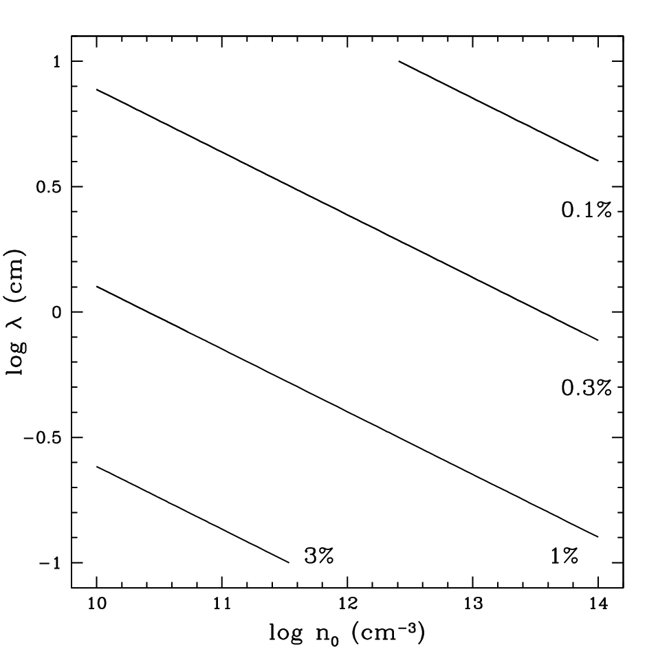
This contribution has explored how synchrotron emission can alter the SED shape formed by a wind that is optically thick to thermal free-free opacity. As discussed above, high opacity results from a combination of dense winds and long wavelength radiation, and the canonical SED shape is a power law with (using the assumption for the Gaunt Factor of adopted throughout this work). This result assumes a spherical, constantly expanding wind. Here, we comment on the applicability of this assumption.
Consider a canonical wind velocity law with , such that . In normalized form, applying the substitution , the velocity law can be expressed as . The optical depth to any location in the wind (eq. [6]), is then
| (C1) |
with
| (C2) |
We note that while is an analytic function of , the determinate of is implicit, requiring root finder methods for a solution.
For constant expansion, the characteristic radius of the free-free photosphere (eq. [8]) is then
| (C3) |
where the location has been defined by the condition of optical unity (eq. [7]).
One way to assess the applicability of our assumptions is to evaluate using eq. (C1). We define the relative error in the approximation for the optical depth as
| (C4) |
Fig. (3) provides a contour plot of this error. For simplicity, we assume a constant stellar luminosity , and have adopted the scaling relations for hot massive star winds from Vink 2021, with , for stellar mass and effective temperature and , respectively (see eq. [4] of that paper). We assume for massive stars that , and constant luminosity implies . For the wind terminal speed, . We apply these scaling relations to eq. (9) to obtain the wind density scale in terms of these quantities,
| (C5) |
Since the most luminous stars tend to have the highest wind mass-loss rates, the assumption of a constant implies , and thus . This is the scaling relation used in Fig. 3. While crude, the relation indicates that lower wind densities correspond to larger stars. For example, a wind density scale of cm-3 and a stellar radius is appropriate to describe a WR star. In contrast, under our assumptions, a density scale of cm-3 (appropriate for an O supergiant) would have a corresponding stellar radius of (which in reality is about a factor of two too large). Overall, Fig. 3 reveals that across the span of wind density scales appropriate to stars ranging from O supergiants to WRs, at wavelengths from around 10 cm to 1 mm, the approximation of constant expansion is quite good. We find a maximum error in the optical unity assumption of 5%, for mm with cm-3.
References
- Abbott et al. (1986) Abbott, D. C., Beiging, J. H., Churchwell, E., & Torres, A. V. 1986, ApJ, 303, 239, doi: 10.1086/164070
- Abbott et al. (1981) Abbott, D. C., Bieging, J. H., & Churchwell, E. 1981, ApJ, 250, 645, doi: 10.1086/159412
- Abbott et al. (1980) Abbott, D. C., Bieging, J. H., Churchwell, E., & Cassinelli, J. P. 1980, ApJ, 238, 196, doi: 10.1086/157973
- Alecian et al. (2014) Alecian, E., Kochukhov, O., Petit, V., et al. 2014, A&A, 567, A28, doi: 10.1051/0004-6361/201323286
- Babel & Montmerle (1997a) Babel, J., & Montmerle, T. 1997a, ApJ, 485, L29, doi: 10.1086/310806
- Babel & Montmerle (1997b) —. 1997b, A&A, 323, 121
- Benaglia et al. (2015) Benaglia, P., Marcote, B., Moldón, J., et al. 2015, A&A, 579, A99, doi: 10.1051/0004-6361/201425595
- Berghoefer et al. (1997) Berghoefer, T. W., Schmitt, J. H. M. M., Danner, R., & Cassinelli, J. P. 1997, A&A, 322, 167
- Bieging et al. (1989) Bieging, J. H., Abbott, D. C., & Churchwell, E. B. 1989, ApJ, 340, 518, doi: 10.1086/167414
- Blomme et al. (2017) Blomme, R., Fenech, D. M., Prinja, R. K., Pittard, J. M., & Morford, J. C. 2017, A&A, 608, A69, doi: 10.1051/0004-6361/201731403
- Blomme & Runacres (1997) Blomme, R., & Runacres, M. C. 1997, A&A, 323, 886
- Bromm & Larson (2004) Bromm, V., & Larson, R. B. 2004, ARA&A, 42, 79, doi: 10.1146/annurev.astro.42.053102.134034
- Brussaard & van de Hulst (1962) Brussaard, P. J., & van de Hulst, H. C. 1962, Reviews of Modern Physics, 34, 507, doi: 10.1103/RevModPhys.34.507
- Cassinelli & Hartmann (1977) Cassinelli, J. P., & Hartmann, L. 1977, ApJ, 212, 488, doi: 10.1086/155068
- Chen & White (1991) Chen, W., & White, R. L. 1991, ApJ, 366, 512, doi: 10.1086/169586
- Chen & White (1994) —. 1994, Ap&SS, 221, 259, doi: 10.1007/BF01091158
- Daley-Yates et al. (2019) Daley-Yates, S., Stevens, I. R., & ud-Doula, A. 2019, MNRAS, 489, 3251, doi: 10.1093/mnras/stz1982
- De Becker (2018) De Becker, M. 2018, Bulletin de la Societe Royale des Sciences de Liege, 87, 185
- De Becker et al. (2017) De Becker, M., Benaglia, P., Romero, G. E., & Peri, C. S. 2017, A&A, 600, A47, doi: 10.1051/0004-6361/201629110
- Dessart & Owocki (2003) Dessart, L., & Owocki, S. P. 2003, A&A, 406, L1, doi: 10.1051/0004-6361:20030810
- Donati & Landstreet (2009) Donati, J.-F., & Landstreet, J. D. 2009, ARA&A, 47, 333, doi: 10.1146/annurev-astro-082708-101833
- Donati et al. (2006) Donati, J. F., Howarth, I. D., Jardine, M. M., et al. 2006, MNRAS, 370, 629, doi: 10.1111/j.1365-2966.2006.10558.x
- Dougherty et al. (2003) Dougherty, S. M., Pittard, J. M., Kasian, L., et al. 2003, A&A, 409, 217, doi: 10.1051/0004-6361:20031048
- Dougherty & Williams (2000) Dougherty, S. M., & Williams, P. M. 2000, MNRAS, 319, 1005, doi: 10.1046/j.1365-8711.2000.03837.x
- Eichler & Usov (1993) Eichler, D., & Usov, V. 1993, ApJ, 402, 271, doi: 10.1086/172130
- Ellison & Eichler (1985) Ellison, D. C., & Eichler, D. 1985, Phys. Rev. Lett., 55, 2735, doi: 10.1103/PhysRevLett.55.2735
- Falceta-Gonçalves & Abraham (2012) Falceta-Gonçalves, D., & Abraham, Z. 2012, MNRAS, 423, 1562, doi: 10.1111/j.1365-2966.2012.20978.x
- Fossati et al. (2015) Fossati, L., Castro, N., Schöller, M., et al. 2015, A&A, 582, A45, doi: 10.1051/0004-6361/201526725
- Fullerton et al. (2006) Fullerton, A. W., Massa, D. L., & Prinja, R. K. 2006, ApJ, 637, 1025, doi: 10.1086/498560
- Gagné et al. (2005) Gagné, M., Oksala, M. E., Cohen, D. H., et al. 2005, ApJ, 628, 986, doi: 10.1086/430873
- Grunhut et al. (2017) Grunhut, J. H., Wade, G. A., Neiner, C., et al. 2017, MNRAS, 465, 2432, doi: 10.1093/mnras/stw2743
- Heger et al. (2003) Heger, A., Fryer, C. L., Woosley, S. E., Langer, N., & Hartmann, D. H. 2003, ApJ, 591, 288, doi: 10.1086/375341
- Heger & Woosley (2010) Heger, A., & Woosley, S. E. 2010, ApJ, 724, 341, doi: 10.1088/0004-637X/724/1/341
- Hopkins et al. (2012) Hopkins, P. F., Quataert, E., & Murray, N. 2012, MNRAS, 421, 3522, doi: 10.1111/j.1365-2966.2012.20593.x
- Huenemoerder et al. (2015) Huenemoerder, D. P., Gayley, K. G., Hamann, W. R., et al. 2015, ApJ, 815, 29, doi: 10.1088/0004-637X/815/1/29
- Hummer (1988) Hummer, D. G. 1988, ApJ, 327, 477, doi: 10.1086/166210
- Ignace (2001) Ignace, R. 2001, ApJ, 549, L119, doi: 10.1086/319141
- Ignace (2016) —. 2016, MNRAS, 457, 4123, doi: 10.1093/mnras/stw216
- Ignace et al. (1998) Ignace, R., Cassinelli, J. P., & Bjorkman, J. E. 1998, ApJ, 505, 910, doi: 10.1086/306189
- Ignace et al. (2013) Ignace, R., Gayley, K. G., Hamann, W. R., et al. 2013, ApJ, 775, 29, doi: 10.1088/0004-637X/775/1/29
- Ignace et al. (2003) Ignace, R., Quigley, M. F., & Cassinelli, J. P. 2003, ApJ, 596, 538, doi: 10.1086/377597
- Klement et al. (2017) Klement, R., Carciofi, A. C., Rivinius, T., et al. 2017, A&A, 601, A74, doi: 10.1051/0004-6361/201629932
- Kochukhov et al. (2011) Kochukhov, O., Lundin, A., Romanyuk, I., & Kudryavtsev, D. 2011, ApJ, 726, 24, doi: 10.1088/0004-637X/726/1/24
- Kurapati et al. (2017) Kurapati, S., Chandra, P., Wade, G., et al. 2017, MNRAS, 465, 2160, doi: 10.1093/mnras/stw2838
- Lamers & Cassinelli (1996) Lamers, H. J. G. L. M., & Cassinelli, I. P. 1996, in Astronomical Society of the Pacific Conference Series, Vol. 98, From Stars to Galaxies: the Impact of Stellar Physics on Galaxy Evolution, ed. C. Leitherer, U. Fritze-von-Alvensleben, & J. Huchra, 162
- Langer (2012) Langer, N. 2012, ARA&A, 50, 107, doi: 10.1146/annurev-astro-081811-125534
- Leitherer et al. (1995) Leitherer, C., Chapman, J. M., & Koribalski, B. 1995, ApJ, 450, 289, doi: 10.1086/176140
- Leitherer et al. (1997) —. 1997, ApJ, 481, 898, doi: 10.1086/304096
- Leto et al. (2006) Leto, P., Trigilio, C., Buemi, C. S., Umana, G., & Leone, F. 2006, A&A, 458, 831, doi: 10.1051/0004-6361:20054511
- Leto et al. (2017) Leto, P., Trigilio, C., Oskinova, L., et al. 2017, MNRAS, 467, 2820, doi: 10.1093/mnras/stx267
- Leto et al. (2018) Leto, P., Trigilio, C., Oskinova, L. M., et al. 2018, MNRAS, 476, 562, doi: 10.1093/mnras/sty244
- Leto et al. (2021) Leto, P., Trigilio, C., Krtička, J., et al. 2021, MNRAS, 507, 1979, doi: 10.1093/mnras/stab2168
- Lucy & White (1980) Lucy, L. B., & White, R. L. 1980, ApJ, 241, 300, doi: 10.1086/158342
- Madau & Dickinson (2014) Madau, P., & Dickinson, M. 2014, ARA&A, 52, 415, doi: 10.1146/annurev-astro-081811-125615
- Morel et al. (2015) Morel, T., Castro, N., Fossati, L., et al. 2015, in New Windows on Massive Stars, ed. G. Meynet, C. Georgy, J. Groh, & P. Stee, Vol. 307, 342–347, doi: 10.1017/S1743921314007054
- Nazé et al. (2014) Nazé, Y., Petit, V., Rinbrand, M., et al. 2014, ApJS, 215, 10, doi: 10.1088/0067-0049/215/1/10
- Nazé et al. (2011) Nazé, Y., Broos, P. S., Oskinova, L., et al. 2011, ApJS, 194, 7, doi: 10.1088/0067-0049/194/1/7
- Nugis et al. (1998) Nugis, T., Crowther, P. A., & Willis, A. J. 1998, A&A, 333, 956
- Oskinova et al. (2012) Oskinova, L. M., Gayley, K. G., Hamann, W. R., et al. 2012, ApJ, 747, L25, doi: 10.1088/2041-8205/747/2/L25
- Oskinova et al. (2011a) Oskinova, L. M., Hamann, W.-R., Cassinelli, J. P., Brown, J. C., & Todt, H. 2011a, Astronomische Nachrichten, 332, 988, doi: 10.1002/asna.201111602
- Oskinova et al. (2011b) Oskinova, L. M., Todt, H., Ignace, R., et al. 2011b, MNRAS, 416, 1456, doi: 10.1111/j.1365-2966.2011.19143.x
- Owocki et al. (1988) Owocki, S. P., Castor, J. I., & Rybicki, G. B. 1988, ApJ, 335, 914, doi: 10.1086/166977
- Owocki & ud-Doula (2004) Owocki, S. P., & ud-Doula, A. 2004, ApJ, 600, 1004, doi: 10.1086/380123
- Panagia & Felli (1975) Panagia, N., & Felli, M. 1975, A&A, 39, 1
- Parkin et al. (2014) Parkin, E. R., Pittard, J. M., Nazé, Y., & Blomme, R. 2014, A&A, 570, A10, doi: 10.1051/0004-6361/201423833
- Pittard et al. (2006) Pittard, J. M., Dougherty, S. M., Coker, R. F., O’Connor, E., & Bolingbroke, N. J. 2006, A&A, 446, 1001, doi: 10.1051/0004-6361:20053649
- Pittard et al. (2021) Pittard, J. M., Romero, G. E., & Vila, G. S. 2021, MNRAS, 504, 4204, doi: 10.1093/mnras/stab1107
- Puls et al. (2006) Puls, J., Markova, N., Scuderi, S., et al. 2006, A&A, 454, 625, doi: 10.1051/0004-6361:20065073
- Rybicki & Lightman (1986) Rybicki, G. B., & Lightman, A. P. 1986, Radiative Processes in Astrophysics (Wiley-VCH), 400
- Schmid-Burgk (1982) Schmid-Burgk, J. 1982, A&A, 108, 169
- Schmutz & Koenigsberger (2019) Schmutz, W., & Koenigsberger, G. 2019, A&A, 624, L3, doi: 10.1051/0004-6361/201935094
- Shultz et al. (2022) Shultz, M. E., Owocki, S. P., ud-Doula, A., et al. 2022, arXiv e-prints, arXiv:2201.05512. https://arxiv.org/abs/2201.05512
- Silvester et al. (2014) Silvester, J., Kochukhov, O., & Wade, G. A. 2014, MNRAS, 440, 182, doi: 10.1093/mnras/stu306
- St-Louis et al. (2020) St-Louis, N., Moffat, A. F. J., Ramiaramanantsoa, T., & Lenoir-Craig, G. 2020, in Stars and their Variability Observed from Space, ed. C. Neiner, W. W. Weiss, D. Baade, R. E. Griffin, C. C. Lovekin, & A. F. J. Moffat, 423–426
- Sundqvist et al. (2018) Sundqvist, J. O., Owocki, S. P., & Puls, J. 2018, A&A, 611, A17, doi: 10.1051/0004-6361/201731718
- Sundqvist & Puls (2018) Sundqvist, J. O., & Puls, J. 2018, A&A, 619, A59, doi: 10.1051/0004-6361/201832993
- Trigilio et al. (2004) Trigilio, C., Leto, P., Umana, G., Leone, F., & Buemi, C. S. 2004, A&A, 418, 593, doi: 10.1051/0004-6361:20040060
- ud-Doula & Nazé (2016) ud-Doula, A., & Nazé, Y. 2016, Advances in Space Research, 58, 680, doi: 10.1016/j.asr.2015.09.025
- ud-Doula & Owocki (2002) ud-Doula, A., & Owocki, S. P. 2002, ApJ, 576, 413, doi: 10.1086/341543
- Van Loo et al. (2004) Van Loo, S., Runacres, M. C., & Blomme, R. 2004, A&A, 418, 717, doi: 10.1051/0004-6361:20034480
- Van Loo et al. (2005) —. 2005, A&A, 433, 313, doi: 10.1051/0004-6361:20041973
- Van Loo et al. (2006) —. 2006, A&A, 452, 1011, doi: 10.1051/0004-6361:20054266
- Vink (2021) Vink, J. S. 2021, arXiv e-prints, arXiv:2109.08164. https://arxiv.org/abs/2109.08164
- Wade et al. (2016) Wade, G. A., Neiner, C., Alecian, E., et al. 2016, MNRAS, 456, 2, doi: 10.1093/mnras/stv2568
- White (1985) White, R. L. 1985, ApJ, 289, 698, doi: 10.1086/162933
- White & Chen (1992) White, R. L., & Chen, W. 1992, ApJ, 387, L81, doi: 10.1086/186310
- White & Chen (1994) —. 1994, Ap&SS, 221, 295, doi: 10.1007/BF01091161
- Williams et al. (1994) Williams, P. M., van der Hucht, K. A., & Spoelstra, T. A. T. 1994, A&A, 291, 805
- Woosley et al. (2002) Woosley, S. E., Heger, A., & Weaver, T. A. 2002, Reviews of Modern Physics, 74, 1015, doi: 10.1103/RevModPhys.74.1015
- Wright & Barlow (1975) Wright, A. E., & Barlow, M. J. 1975, MNRAS, 170, 41, doi: 10.1093/mnras/170.1.41