Accelerating phase-field-based simulation via machine learning
Abstract
Phase-field-based models have become common in material science, mechanics, physics, biology, chemistry, and engineering for the simulation of microstructure evolution. Yet, they suffer from the drawback of being computationally very costly when applied to large, complex systems. To reduce such computational costs, a Unet-based artificial neural network is developed as a surrogate model in the current work. Training input for this network is obtained from the results of the numerical solution of initial-boundary-value problems (IBVPs) based on the Fan-Chen model for grain microstructure evolution. In particular, about 250 different simulations with varying initial order parameters are carried out and 200 frames of the time evolution of the phase fields are stored for each simulation. The network is trained with 90% of this data, taking the -th frame of a simulation, i.e. order parameter field, as input, and producing the -th frame as the output. Evaluation of the network is carried out with a test dataset consisting of 2200 microstructures based on different configurations than originally used for training. The trained network is applied recursively on initial order parameters to calculate the time evolution of the phase fields. The results are compared to the ones obtained from the conventional numerical solution in terms of the errors in order parameters and the system’s free energy. The resulting order parameter error averaged over all points and all simulation cases is 0.005 and the relative error in the total free energy in all simulation boxes does not exceed 1%.
Keywords— Machine learning, Deep learning, Convolutional neural network, U-Net, Phase-Field, Grain growth, Allen-Cahn, Fan-Chen
1 Introduction
Over the past decades, phase-field (PF) approaches have become one of the most common methods for computational modeling and simulation of microstructure evolution in materials science and engineering as well as several other disciplines [1, 2, 3, 4, 5, 6, 7]. In the case of metallic alloy systems, PF-based models have been developed for a number of phenomena including solidification, structural phase transformation, chemical species transport, precipitation, defects, and plasticity, or recrystallization, mostly aiming at the prediction of microstructure evolution at the mesoscale [8, 9, 10, 11, 12, 13, 14, 15, 16, 7, 17].
In PF-based models for metallic alloys, the phases, their associated microstructures, and chemical composition are described by PFs that vary smoothly across phase interfaces. The energy landscape of the material, from which local driving forces are derived, is parameterized by the PFs, or the order parameters in the case of non-conservative phase fields. In the case of metallic alloys, PF-based models are either of Cahn-Hilliard (CH) type [18, 19] for conservative phase fields (e.g., chemical concentration) or Allen-Cahn (AC) [20, 21] type for non-conservative phase fields (e.g., structural order parameters).
Although PF-based models can describe microstructure evolution in a broad range of physical, biological, and chemical systems, the corresponding computational efforts required to solve them are often prohibitively expensive. The reasons for this include (i) the fine spatial and temporal discretization required for a converged (i.e., physical) solution of the corresponding initial-boundary-value problems (IBVPs) and (ii) iteration-based and often staggered numerical schemes to solve the underlying partial differential equations. Particularly in the case of coupled multi-physics models (where for instance structural, mechanical, and chemical fields must be considered), these are principle obstacles to the simulation of microstructure evolution, especially in systems much larger than the currently tackled microstructural lengthscales. In the multiphysics case, multiple material lengthscales need to be resolved in the same spatial domain during simulation based on the numerical solution of the corresponding coupled IBVPs. Such multiphysics cases in materials science and engineering include Li-ion batteries, hydrogen embrittlement, stress corrosion cracking, iron-ore reduction, or solidification, which involve a non-linear interplay of microstructure, chemistry, and mechanics. Finding ways to reduce the computational effort required for the PF-based computational modeling and simulation of such cases is essential for the extension of the PF approach to even larger and more complex systems. The core idea behind this is not simply to be able to deal with larger system sizes but to properly reflect the different coherence lengths involved in the respective fields (such as interface density, dislocation density, grain size, diffusion length, etc.). Also, the behavior of certain complex systems is often hidden behind the interplay of structure, mechanics, and chemistry. This means that the coupling that enters through multi-physics simulations and the system size becomes integral tasks of the proper formulation of the actual scientific problem addressed.
A number of steps have been taken to tackle this challenge; for example, developing more efficient numerical techniques [22, 23], parallel computing, or employing graphics processing units (GPU). Despite the success of these, the ever-increasing computational complexity, required system size, and number of variables, require even further increase in computational speed [24, 25, 26]. As a result, alternative approaches such as machine learning (ML) have received a lot of attention in recent years.
ML offers a range of powerful techniques, some of which have been applied in computational materials science [27, 28, 29]. Currently, many studies are focusing on applying ML in different areas of materials science [29, 30]. One recent application of ML in this regard is the development of so-called surrogate computational models based on trained artificial neural networks (tANNs). For instance, Mianroodi et al. [25] developed an ANN for surrogate computational modeling of the stress field in a grain microstructure consisting of elastoplastic single crystals. They demonstrated that the calculation of the stress field using the tANN-based surrogate model is up to 8000 times faster than the spectral-based numerical solution of the corresponding periodic IBVP, even for grain microstructures not included in the training data set. In a different context, Nyshadham et al. [31] developed a fast surrogate model to estimate the properties of materials such as elastic constants, enthalpy, and band-gap, with the accuracy of ab initio methods. In addition, surrogate models have also been employed in up-scaling of multi-scale systems (see [32, 33, 34]).
In the case of PF-based modeling, several attempts have been made to develop surrogate models for the evolution of chemical composition and structural order parameter fields based on spatio-temporal pattern correlation. Recently, Montes de Oca Zapiain et al. [35] presented a new data-driven surrogate model capable of predicting microstructure evolution in less than a second. They used a long-short-term memory network trained with results from the numerical solution of a physical IBVP. Comparison of results from their surrogate model for spinodal decomposition with those from the solution of the IBVP show 95% agreement. Zhang et al. [36] developed a surrogate model based on deep neural networks (DNNs) and convolutional neural networks (CNNs) trained using free energy fluctuations and used this to calculate the stress in their microstructure. They showed that both CNN-based and DNN-based neural network architectures are performing equally in capturing microstructure features and predicting free energy evolution. Teichert and Garikipati [37] carried out similar work in which DNNs were trained with free energy results from the numerical solution of a PF-model-based IBVP and employed in the surrogate modeling of precipitate morphology. In another study, Hermen et al. [38] developed a trained ANN based on results for chemical vapor deposition and applied this to the surrogate modeling of a corresponding microstructure. Similar surrogate models have been developed in [39, 40, 41].
Evaluation of surrogate models is often based on three criteria [24]: (i) size of the training dataset, (ii) time needed to train a neural network and obtain results, and (iii) model accuracy. In particular, (i) and (ii) are related to the efficiency of the training process. As usual, there is a trade-off between efficiency and accuracy, and so a need for further optimization, i.e., to reduce (i) and (ii) while maintaining (iii). In other words, a need exists to develop fast and accurate surrogate models based on training datasets of minimal size and training effort.
In this study, we develop a surrogate model trained with results from the numerical solution of IBVPs based on the Fan-Chen model for grain growth [42] and semi-implicit spectral methods. The resulting model is capable of calculating the change in order-parameter fields that represent the microstructure evolution at many timesteps forward. Compared to other approaches, the method suggested here is a point-wise neural network that requires a considerably smaller dataset (a few hundred microstructure evolution paths) compared to the other neural network architectures. A U-net-based ANN architecture is used in this work. Since the free energy is a functional of the order parameters, it is used as an accuracy measure. Following the introduction, the work begins in Section 2 with a summary of the Fan-Chen model and its numerical implementation. Based on this, Section 3 discusses the training dataset. In Section 4, the ANN architecture, input and output, and training are discussed. Evaluation of the resulting tANN-based surrogate model is carried out in Section 5 with the help of a number of comparison measures (e.g., the free energy) and benchmark cases for microstructure evolution. Besides on accuracy, emphasis is placed here on the increase in computational speed achieved. Finally, in Section 6, we draw conclusions and discuss future directions for the current work.
2 Fan-Chen model and numerical implementation
2.1 Model
Grain growth is an important and often property-critical phenomenon in metallurgy [43]. In conventional grain growth, grain boundaries move due to local capillary forces acting on them, minimizing the system’s total free energy, stemming in this case from the interfacial energy. Grain growth is of paramount importance owing to its impact on material properties [44, 45]. Consequently, it has been studied substantially from atomistic to continuum scales [46, 47, 45, 48]. At the mesoscale, several models have been proposed to simulate this phenomenon by using the PF method. One of the well-known and commonly used models is the Fan-Chen model [42]. In this model, each connected domain of the same crystallographic orientation, referred to as a grain, is represented by one specific non-conserved structural order parameter (or field variable) which is 1 inside the grain and 0 in all other grains. For example, in grain number 2, assumes the value 1, and in all other grains it is 0, changing its value smoothly across grain boundaries. Interested readers are referred to [42] for more details about the model. The evolution of order parameters () takes place by the non-conservative Allen–Cahn equation (or, respectively, the time-dependent Ginzburg-Landau equation)
| (1) |
where is the number of grains, is the mobility, is time, and
| (2) |
is the free energy functional. In (2), is the local free energy, and are the gradient energy coefficients, which are taken as constant here. Taking the functional derivative of (2) and combining it with (1), we get
| (3) |
The local free energy is written as
| (4) |
where , and are positive constants.
2.2 Numerical implementation
In this work, the spectral method, in particular, the Fast Fourier Transform (FFT), is chosen as the numerical tool to solve the PDE in (1) and generate high-fidelity reference data for training and testing the artificial neural network. In this method, quantities are transformed from the real space to the reciprocal space as
| (5) |
where is the wave vector. The spatial derivatives in Fourier space are given by
| (6) |
Taking the Fourier transform of the two sides of (3), the reciprocally-discrete equation is
| (7) |
Note that the quantity inside the bracket above must be transformed into Fourier space. consists of and components with a magnitude of . The semi-implicit form of (7) is
| (8) |
where is the timestep size. It is worthwhile to mention that for the forward and the backward transform into and from Fourier space, respectively, fft and ifft functions from the Numpy [49] package in python were used.
3 Data preparation
All parameters are in non-dimensional form. The 2D simulation domain is a square grid with 128 points in and directions ( = 128 and = 128). A grid point spacing of , and a timestep size of , are employed for the numerical solution of Equation (8). In addition, values of 20 and 0.3 are adopted for the relaxation coefficient and the gradient energy coefficient , respectively. Likewise, , and in Equation (4) are all assumed equal to 1.0. The choice of these parameters ensures a numerically well-resolved interface as well as reaching equilibrium before the end of the simulations.
In this study, for simplicity, we only consider binary grain structures. This means that we use only two types of crystals (grains) with homogeneous internal structure, i.e. they have a constant value of the structure variable in their interior, so that a grain is constituted by a homogeneous domain that assumes a value of 1 for one of the two order parameters. Therefore, there are only two order parameters used to describe the microstructure in this domain ( and ). takes a value of 1 in the first grain and 0 in the second one. Likewise, takes the value of 0 in the first grain and 1 in the second grain. The regions where these order parameters assume a value between 0 and 1 are the interface regions. Interface regions contribute an extra energy term to the system, resulting in a driving force for the evolution of the grain boundaries.
Initial order parameter field values in the simulation cell determining initial grain shapes are chosen randomly from a set of images. Fig. 1 depicts 9 different examples of initial configurations of .
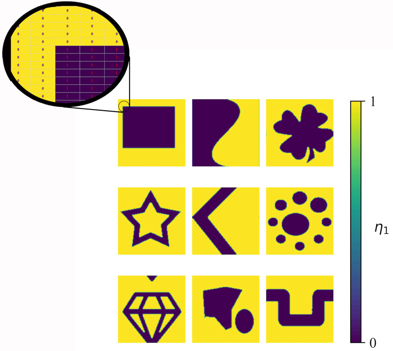
Since the system consists of only two grains, the second order parameter would be . The evolution of each configuration is simulated for 10,000 timesteps, and the solution of (8) for () is stored every 50 timesteps. As a result, the temporal evolution of each initial configuration is captured in the form of 200 subsequent frames. In other words, at the end of each simulation, 200 consecutive solution snapshots are saved, each containing the spatial distribution of the two order parameters in the 2D domain. We eliminate the first snapshot, as it has sharp interfaces and it is far from equilibrium. An example of the full evolution of one microstructure is shown in Fig. 2.
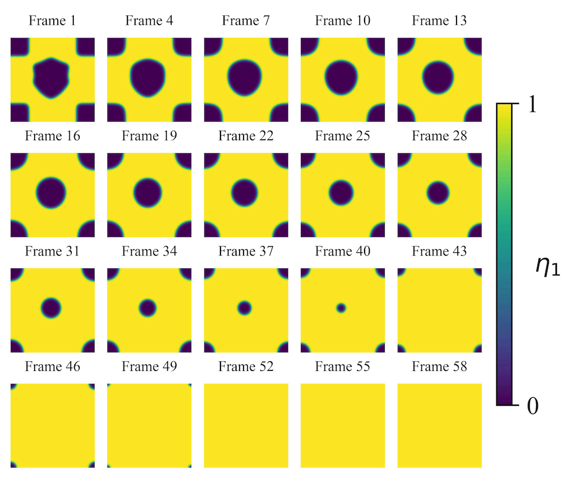
In the end, the 250 initial configurations generate 500,000 frames, each containing the evolving grain growth patterns produced by two order parameters, , and . As shown for example in Fig. 2, one grain grows (yellow in the figure) at the expense of the other during microstructure evolution, resulting in a homogeneous single crystal. In particular, due to concavity, the capillary driving force drives shrinkage of the unstable grain which completely disappears after the frame (or 2500 timesteps). In such cases, only the first two homogeneous solutions have been stored. Our goal is to train the network to reproduce the time-dependent behavior of the microstructure.
4 Neural network architecture and training
Most physical phenomena in materials science can be modeled through solving PDE-based mathematical formulations, hence, any method accelerating their solution is important in this field. In this context, trained ANNs as surrogate models to reproduce the numerical solution of PDEs are very promising.
In the current work, results from the solution of the IBVP discussed in the previous section are used to train an ANN directly, resulting in a tANN-based surrogate model. Our goal is to develop a tANN to reproduce the time evolution of the phase-field order parameter based on the numerical solution of a periodic IBVP based on the Fan-Chen model for grain growth as discussed above. To this end, a ”U-net” architecture [50] is adopted and modified for this purpose. U-net has been mainly used for classification and segmentation in computer vision. Recently, however, Mianroodi et al. [34] trained a U-net-based ANN for surrogate modeling of the stress field in polycrystalline microstructures. In this work, we show that a similar U-net can effectively reproduce results from the spatio-temporal numerical solution of an IBVP based on the Fan-Chen model.
4.1 Neural network architecture
The input to the network in the current context consists of values of order parameter fields for each grain in the microstructure. Since these are naturally dimensionless and take values between 0 and 1, they are ideally suited as training information. For simplicity, attention is limited here to 2 dimensions and a 2-grain or 2-phase microstructure. As such, the input consists of values for two order parameters and at each node/pixel in phase-field simulation domain (with ) discussed above, resulting in the input format shown on the left in Fig. 3.

In each of the 4 encoder stages (Fig. 3, left side, orange), the data are processed by two convolution layers. The padding for each convolution layer is considered the ”same”, so the dimension of any output data is the same as the input data. Convolution layers are based on kernels that are essentially simple filters that identify local pattern features in the training data. They are a core tool in such network architectures for pattern correlation via sequentially applied algebraic matrix operations. Stacking convolution layers in each stage of the encoder facilitates the correlation of important features in the input data. Note that the kernel of the convolution layers has a fixed size (in our case the kernel is a matrix). The components of the kernels are optimized during the training procedure. The activation function used in our network is a Rectified Linear Unit (ReLU). Batch normalization is employed between all convolution steps to compress the data. Downsampling is based on a Max Pooling operation with a stride size of two and a pool size of . As shown in Fig. 3, the input is compressed in the encoder to . This is then input into the decoder and expanded through 4 decoder stages. The skip connections concatenate the output of the corresponding encoder and decoder stages (orange arrows). In the final stage on the right, the resulting data is transformed into the format of the input data. Note that we use the terminology adopted by TensorFlow [51] for the different operations in the network, such as Conv2D (generate convolution kernel), MaxPool2D (downsamples data), and Conv2DTranspose (deconvolution that upsamples data).
4.2 Network input and output
In Section 3, the generation of the dataset has been explained. 250 initial configurations of different spatial patterns (grain microstructures) determined by the order parameter fields in a square domain discretized by 128128 pixels are employed as initial conditions to solve the initial-boundary-value problem (IBVP) based on the Fan-Chen model and Eq. (8) for 10,000 timesteps. The corresponding solutions are saved every 50 timesteps as arrays. Hence, the size and shape of the datasets for two order parameters is . Note that the initial order parameter patterns contain in part random shapes with sharp interfaces, i.e. the interface initially has zero thickness. Therefore, the time evolution of the order parameters in the few first steps of the solution is much faster, due to the large driving force from the gradient term, than during the rest of the simulations. Since we are not interested in sharp interface scenarios in this work, we removed the first frames from all simulations (corresponding to timestep 50) from the training data set. Therefore, the dimension of the dataset becomes . In some simulation cases, one of the grains will shrink and disappear depending on the initial conditions. Once a grain has been annihilated (overgrown), the solution will not evolve anymore as we do not include any nucleation process in this work. Thus, simulation frames with homogeneous order parameter distributions, representing a perfect single crystal, are removed from the database. After filtering such cases, around 22000 microstructures remain in the dataset.
The goal is to train the ANN to output results for the phase fields and microstructure for a given input that are close to those that would be obtained from a numerical solution of the corresponding IBVP based on the Fan-Chen model. An example of such a typical input and output scenario is shown in Fig. 4.

Here, order parameter values for timestep are input to the ANN, and order parameter results for timestep are output.
4.3 Network training
In training and testing ANN, a dataset is typically divided into three parts of (i) training, (ii) validation, and (iii) test datasets. The training dataset is used in optimizing the trainable parameters of the network, while the performance of the network on the validation dataset is monitored during the training to detect over / underfitting. The test dataset is kept separate and only used to evaluate the accuracy of the network after training. In this work, 90% of the entire dataset (randomly selected) has been assigned to training and the remaining 10% to testing. 10% of the training dataset was also considered for validating the neural network. Note that there is a terminology discrepancy between the field of constrained optimization (CO) and machine learning which is explained in the discussions. Here we adopt the common terminology in the field of machine learning. The total number of trainable parameters in the neural network is 487,226. As usual, training is based on minimization of the corresponding objective or ”loss” function, which in this work is the mean absolute error (MAE) between the results from the numerical solution () of the IBVP based on the Fan-Chen model and the corresponding output of the neural network ()
| (9) |
where is the number of all microstructures in the dataset. Monitoring the value of the loss function during network training is a common way to evaluate training. In Fig. 5 (a), the training and validation loss (based on the order parameters) as a function of epochs are reported.

Based on the results in this figure, no sign of over-fitting or under-fitting is observed. Besides the monitored evaluation of the loss function, the quality of training is also examined with respect to the relative error in the free energy displayed in Fig. 5 (b). This error is between 0.001 and 0.002 for both, training and validation. This means that the neural network produces a total free energy value for the respective microstructure at the next desired timestep with high precision.
The ADAM optimizer [53] is employed as the stochastic gradient descent algorithm with the learning rate of . The other parameters of the ADAM optimizer are as follows: , and . The neural network is trained for 64 epochs and a batch size of 32. These are found to be the optimal training parameters (hyperparameters) in our case, resulting in the smallest values of the loss function after training. The free energy (which quantifies all interface energy contributions in the Fan-Chen model, see (4)) is defined as an important metric for evaluating the neural network. The derivatives of the free energy with respect to the order parameters are the driving force for the evolution of the phase fields. After each epoch, the network compares the mean relative error between the results from the numerical solution of the Fan-Chen model and the one calculated by the neural network. The training takes about 30 minutes with a GeForce GTX 1060 GPU (compute capabilities = 6.1).
5 Results and discussion
In the first evaluation, we investigate the effect of the timesteps on the neural network’s performance. For this purpose, we train the same network three times to reproduce the evolving patterns of the order parameters after 100, 500, and 1000 timesteps. Next, we create new microstructures different from those used for training to investigate the network’s performance on unseen microstructures. Finally, we evaluate the neural network’s capability in determining the entire time series. In this case, the network’s output is used again as the input for calculating results for several timesteps.
5.1 Neural network output for one frame forward
As outlined above, the neural network can be trained to reproduce the solution of the Fan-Chen model at any desired timestep, Fig. 6 compares three models of the network that are trained to reproduce solutions after three different timesteps.

In this figure, (a) is the initial configuration of the order parameters. Note that the neural network has not seen this shape in the training process. Column (I) shows the microstructure after 100 timesteps, column (II) after 500 timesteps, and column (III) after 1000 timesteps (the timestep size is 0.008). Row (b) displays results from the neural network, row (c) from the numerical solution of the Fan-Chen model, and row (d) illustrates the error between the neural network and the numerical solution of the Fan-Chen model. It appears that as we increase the jump forward to the next timestep from 100 to 1000, the error goes up slightly in some particular areas of the microstructure, namely, at the grain boundaries, where the order parameters change from 1 to 0 and vice versa. However, the mean absolute error for three cases remains close (0.0011 for I, 0.0015 for II and 0.0021 for III). Furthermore, the relative error in total free energy for all three cases is around 0.002. We can conclude from this that choosing larger steps in the order parameter calculation has a limited impact on the error or overall performance of the neural network. In the rest of this work, we test the trained network to reproduce 500 timesteps forward with other microstructures, specifically with those that had not been included in the training dataset. Fig. 7 depicts four examples of order parameter output after 500 timesteps forward.

Fig. 7 (a) shows the configuration of the order parameter at timestep (). The evolution of (a) after 500 timesteps (i.e., ) is shown in (b) and (c) as output by the trained neural network and by the numerical solution of the Fan-Chen model, respectively. Row (d) shows the error between the results of the neural network and the numerical solution of the Fan-Chen model. Evidently, those output by the network agree well with those from the numerical solution of the Fan-Chen model. We also calculate the free energy of both cases, (b) and (c) through equation 4. The results are presented in table 1.
| Cases | I | II | III | IV |
|---|---|---|---|---|
| Free Energy, Fan-Chen model | -2750.24 | -3328.13 | -1258.49 | -2771.49 |
| Free Energy, trained network | -2747.93 | -3326.04 | -1254.87 | -2767.07 |
| MAE | 2.311 | 2.085 | -3.62 | 4.42 |
| MRE (%) | 0.08 | 0.06 | 0.28 | 0.15 |
The case (I) in Fig. 7 shows a grain inside another grain. Such topological scenarios are straightforward for the neural network to reproduce since just two grains exist, no box boundaries are involved, and the area occupied by grain number 1 (yellow) is larger than that of grain number 2. The neural network handles large curvatures (translating to a large capillary driving force in the Fan-Chen model) in this microstructure very well. Although the error in the order parameter in some areas of the microstructure reaches 0.07, the mean absolute error remains below 0.0013 over the whole domain. The mean relative error in the free energy for this case is 0.08%, showing that the network’s performance in such cases is excellent.
Case (II) in Fig. 7 shows a microstructure in which the area of grain 2 remains constant, and the microstructure does not change over time. This case shows that the neural network recognizes this special case very well. The maximum absolute error in the order parameter is 0.05, and the relative error on the free energy is 0.06%.
The third example, i.e., case (III) in Fig. 7 is another special case in which multiple grains with the same order parameter are inside each other. In this scenario, the grain with the lowest area shrinks faster than the others. The absolute error in some areas near the box boundary reaches 0.08, while in the grain boundaries, it is less than 0.04 and in the whole domain, the mean absolute error is below 0.0016. The value of the relative error on the free energy is 0.28%, which indicates that the neural network also outputs the microstructures accurately.
The fourth example, case (IV) in Fig. 7, is a scenario with two grains close to each other with concave and convex boundaries, respectively. In this configuration, these close grains merge instead of shrinking individually. Even though the absolute error in some points reaches 0.10, in other areas of the grain boundary, it is less than 0.02. The mean relative error of 0.15% for the free energy indicates that the neural network can accurately reproduce the evolution of the order parameter in this case as well.
In addition to the special cases discussed above, we also made comparisons for all microstructures in the test dataset consisting of 2000 different microstructures. The mean absolute error in the order parameter in our test dataset is less than 0.003. However, at the boundaries of the microstructures, it might reach around 0.1 in a few points. The relative error in the free energy can reach 1.0% in a few special cases, while it remains below 0.1% for most cases in the test dataset. This shows that the trained neural network output for the order parameter evolution is quite accurate after 500 timesteps. Next, we investigate the application of the same neural network recursively to reproduce the whole time series of the order parameters evolution.
5.2 Neural network output for time series
The neural network outputs the next desired timestep with reasonable accuracy, as described in the previous section. The network’s output can be fed again to the input recursively to reproduce the order parameter’s whole time evolution. Fig. 8 shows the temporal evolution of the three different microstructures according to the Fan-Chen model. We choose here grain microstructures different from those used in the training and testing process.

Fig. 8 (a1) shows the initial condition of a conventional microstructure, containing two grains. (b1) shows the evolution of (a1) as calculated by the neural network. (c1) shows the microstructure evolution of the starting configurations (a1), calculated by solving the PDEs of the Fan-Chen model numerically (as explained in the Methods section), where is shown after 500, 1000, 2000, 3000, and 3500 timesteps. The error in the trained network output is depicted in (d1). The result shows that the error accumulates slowly after each prediction, and at the end of the simulation, it goes up to 0.1 in some of the points in the domain, while the mean absolute error during the simulation drops from 0.0017 to 0.0010. (e1) also compares the total free energy of the domain, calculated based on the gradients of the order parameters at the interfaces. The error accumulation in the total free energy is quite small, reaching only 0.17% during the simulation. This result indicates that the accuracy of the network output is still quite high for time series prediction.
The second example, as shown in Fig. 8 (a2), considers two grains in the domain as in the preceding example, but this time one of them contains a secondary smaller grain. The temporal evolution of this scenario obtained from the neural network output and the numerical solution of the Fan-Chen model is shown in (b2) and (c2), respectively. (d2) shows the error, which in this case increases up to 0.15 at the end of the simulation. (e2) shows the free energy of the microstructure, calculated based again on the transition regions of the order parameters marking the interface regions. The maximum relative error on the free energy accumulating during the simulation between the two methods is 0.25%.
The last case (a3) in Fig. 8 shows an initial configuration of a complicated microstructure far from the dataset used to train the neural network. As described in the previous section, first, the grain with the smaller area shrinks and disappears, and then the grain with the largest area absorbs the other one. Both methods reproduce this trend correctly, as shown for the neural network output in in (b3) and the numerical solution in (c3). The errors in the order parameter (d3) and in the free energy (e3) illustrate that the neural network is able to reproduce the evolution of this microstructure scenario (a3), which was not included in the training dataset.
5.3 Computational speed
The results shown above demonstrate a good neural network accuracy for the time evolution of the order parameters for a wide variety of microstructural topologies. To investigate the increase in computational speed obtained with the network relative to the conventional forward simulation, we employ one core of an Intel(R) Core(TM)i5 CPU, clocked at 3.2 GHz, for both numerical solution of the Fan-Chen model and neural network output. The neural network calculates the next frame (500 timesteps forward) in 38 milliseconds (measured on average over multiple evaluations), while the FFT solver computes 500 timesteps in 3.448 seconds, meaning that in this case, the neural network calculates the next frame around 90 times faster than the FFT based solver. Note that the computation time for evaluating the microstructure evolution by the trained network is independent of the initial configuration of the order parameters. In contrast, the convergence of the numerical solver highly depends on the complexity of the order parameter distribution. Furthermore, the speedup reported above is merely an estimate. Both, the neural network and the FFT-based calculations could be performed in more efficient ways. For example, here, we focused mainly on output 500 timesteps forward. However, as shown in Fig. 6, with the same amount of calculations, the neural network will also work for output 1000 timestep forward. Similarly, the FFT-based solver could employ advanced adaptive time integration algorithms to speed up the calculations.
6 Conclusions
For a broad range of physical, biological, and chemical systems, the phase-field model provides a powerful and versatile computational methodology suited for calculating the evolution of microstructures and their associated properties. Current phase-field models and numerical methods, however, are computationally expensive by nature, necessitating high-performance computing systems as well as complex numerical integration approaches to obtain a reasonable level of precision. In this study, we presented a fast, efficient and accurate way to reproduce solutions of the Fan-Chen model for grain growth. For this goal, a dataset of non-conserved structural order parameters that define the grain microstructures and their evolution was generated by numerical simulation. A U-net architecture was then used to learn from a subset of these conventional full-field solutions the time-dependent evolution of the patterns (i.e. microstructures) in the dataset. The U-net is a Convolutional Artificial Neural Network architecture that can receive the matrix of order parameters and extract important features in the latent space while transferring the spacial information through skip connections. The trained U-net is then evaluated with the use of the test dataset as well as with special microstructure topology cases that had not been included in the original training dataset. Our findings show that the U-net is able to find the solution to the time-dependent PDE (here Fan-Chen model) by mapping the order parameter in the next desired timestep to the previous one. We trained the U-net on the simulation data with frames generated each 100, 500, and 1000 timesteps. Although larger leaps might be possible, we selected 500 timesteps as a reasonable compromise between error and efficiency. Recursive application of the neural network results in generating the whole time series of the order parameter evolution with minimum accumulated error in our case. Besides the reasonable accuracy of the method, the U-net is shown to be about 90 times faster than the numerical simulation with a mean absolute error of the order parameter and a mean relative error of free energy around 0.0015 and 0.002, respectively. Besides, the solution from the U-net surrogate model can be fed directly into a conventional high-fidelity phase-field model and evolve by numerical simulation to jump in time and speed up the conventional high-fidelity phase-field simulation, opening the opportunity for highly efficient hybrid modeling architectures. We can take advantage of this accelerated framework to quickly explore a large phase-field input domain for all kinds of mesoscale problems that can be described by non-conserved order parameters and the Fan-Chen equation. Future studies on multi-scale and multi-physics simulations will benefit from these findings.
Data availability: The data that support the findings of this study are available from the corresponding author upon reasonable request.
Code availability: The code used for machine learning in this study is open-source and accessible in github.com/tensorflow. Other codes and scripts used in this work are available from the corresponding author upon reasonable request.
Acknowledgement: The support from Shahid Beheshti University is gratefully acknowledged. This research did not receive any specific grant from funding agencies in the public, commercial, or not-for-profit sectors.
Author contributions: I.P., J.R.M. and G.A. developed the initial concept and workflow. I.P. and J.R.M developed the PF and the neural network framework. N.H.S. and R.G. contributed to the neural network design and training approach. I.P. and carried out the PF calculations and neural network training. D.R. , B.S. and G.A. helped in the interpretation of the results. I.P. and J.R.M prepared the initial draft of the manuscript. J.R.M supervised the work. All authors discussed and contributed to preparing the final version of the manuscript.
Competing interests: The authors declare no competing financial or non-financial interests.
References
- [1] Mannor, S., Peleg, D. & Rubinstein, R. The cross entropy method for classification. In Proceedings of the 22nd International Conference on Machine Learning, ICML ’05, 561–568 (Association for Computing Machinery, New York, NY, USA, 2005).
- [2] Chen, L.-Q. Phase-field models for microstructure evolution. Annu. Rev. Mater. Res. 32, 113–140 (2002).
- [3] Biner, S. B. An Overview of the Phase-Field Method and Its Formalisms, 1–7 (Springer International Publishing, Cham, 2017).
- [4] Boettinger, W. J., Warren, J. A., Beckermann, C. & Karma, A. Phase-field simulation of solidification. Annu. Rev. Mater. Res. 32, 163–194 (2002).
- [5] Steinbach, I. Phase-field models in materials science. Model. Simul. Mater. Sci. Eng. 17, 073001 (2009).
- [6] Porter, D. A. & Easterling, K. E. Phase transformations in metals and alloys (revised reprint) (CRC press, 2009).
- [7] Chen, L.-Q. Phase-field models for microstructure evolution. Annu. Rev. Mater. Res. 32, 113–140 (2002).
- [8] Li, Y., Hu, S., Sun, X. & Stan, M. A review: applications of the phase field method in predicting microstructure and property evolution of irradiated nuclear materials. Npj Comput. Mater. 3, 1–17 (2017).
- [9] Millett, P. C. & Tonks, M. Application of phase-field modeling to irradiation effects in materials. Curr. Opin. Solid. State Mater. Sci. 15, 125–133 (2011).
- [10] Tonks, M. R., Cheniour, A. & Aagesen, L. How to apply the phase field method to model radiation damage. Comput. Mater. Sci. 147, 353–362 (2018).
- [11] Ambati, M., Gerasimov, T. & De Lorenzis, L. A review on phase-field models of brittle fracture and a new fast hybrid formulation. Comput. Mech. 55, 383–405 (2015).
- [12] Cervera, M., Barbat, G., Chiumenti, M. & Wu, J.-Y. A comparative review of xfem, mixed fem and phase-field models for quasi-brittle cracking. Arch. Comput. Methods Eng. 1–75 (2021).
- [13] Steinbach, I. Why solidification? why phase-field? Jom 65, 1096–1102 (2013).
- [14] Mamivand, M., Zaeem, M. A. & El Kadiri, H. A review on phase field modeling of martensitic phase transformation. Comput. Mater. Sci. 77, 304–311 (2013).
- [15] Bui, T. Q. & Hu, X. A review of phase-field models, fundamentals and their applications to composite laminates. Eng. Fract. Mech. 107705 (2021).
- [16] Tonks, M. R. & Aagesen, L. K. The phase field method: mesoscale simulation aiding material discovery. Annu. Rev. Mater. Res. 49, 79–102 (2019).
- [17] Singer-Loginova, I. & Singer, H. The phase field technique for modeling multiphase materials. Rep. Prog. Phys. 71, 106501 (2008).
- [18] Cahn, J. W. & Hilliard, J. E. Free energy of a nonuniform system. i. interfacial free energy. J. Chem. Phys. 28, 258–267 (1958).
- [19] Cahn, J. W. On spinodal decomposition. Acta metallurgica 9, 795–801 (1961).
- [20] Allen, S. M. & Cahn, J. W. Ground state structures in ordered binary alloys with second neighbor interactions. Acta Metallurgica 20, 423–433 (1972).
- [21] Allen, S. M. & Cahn, J. W. A correction to the ground state of fcc binary ordered alloys with first and second neighbor pairwise interactions. Scripta Metallurgica 7, 1261–1264 (1973).
- [22] Cheng, Y., Kurganov, A., Qu, Z. & Tang, T. Fast and stable explicit operator splitting methods for phase-field models. J. Comput. Phys. 303, 45–65 (2015).
- [23] Tang, T. On effective numerical methods for phase-field models. Proceedings of the International Congress of Mathematicians (ICM 2018) (2019).
- [24] Alizadeh, R., Allen, J. K. & Mistree, F. Managing computational complexity using surrogate models: a critical review. Res. Eng. Des. 31, 275–298 (2020).
- [25] Mianroodi, J. R., Siboni, N. H. & Raabe, D. Teaching solid mechanics to artificial intelligence—a fast solver for heterogeneous materials. Npj Comput. Mater. 7, 1–10 (2021).
- [26] Li, Z.-Y. et al. Fourier neural operator for parametric partial differential equations. ArXiv abs/2010.08895 (2021).
- [27] Huang, J., Liew, J., Ademiloye, A. & Liew, K. M. Artificial intelligence in materials modeling and design. Arch. Comput. Methods Eng. 28, 3399–3413 (2021).
- [28] Ward, L. et al. Strategies for accelerating the adoption of materials informatics. MRS Bull. 43, 683–689 (2018).
- [29] Schmidt, J., Marques, M. R., Botti, S. & Marques, M. A. Recent advances and applications of machine learning in solid-state materials science. Npj Comput. Mater. 5, 1–36 (2019).
- [30] Ward, L. & Wolverton, C. Atomistic calculations and materials informatics: A review. Curr. Opin. Solid. State Mater. Sci. 21, 167–176 (2017).
- [31] Nyshadham, C. et al. Machine-learned multi-system surrogate models for materials prediction. Npj Comput. Mater. 5, 1–6 (2019).
- [32] Peng, G. C. et al. Multiscale modeling meets machine learning: What can we learn? Arch. Comput. Methods Eng. 28, 1017–1037 (2021).
- [33] Wang, K. & Sun, W. A multiscale multi-permeability poroplasticity model linked by recursive homogenizations and deep learning. Comput. Methods Appl. Mech. Eng. 334, 337–380 (2018).
- [34] Mianroodi, J. R., Rezaei, S., Siboni, N. H., Xu, B.-X. & Raabe, D. Lossless multi-scale constitutive elastic relations with artificial intelligence. Npj Comput. Mater. 8, 67 (2022).
- [35] de Oca Zapiain, D. M., Stewart, J. A. & Dingreville, R. Accelerating phase-field-based microstructure evolution predictions via surrogate models trained by machine learning methods. Npj Comput. Mater. 7, 1–11 (2021).
- [36] Zhang, X. & Garikipati, K. Machine learning materials physics: Multi-resolution neural networks learn the free energy and nonlinear elastic response of evolving microstructures. Comput. Methods Appl. Mech. Eng. 372, 113362 (2020).
- [37] Teichert, G. H. & Garikipati, K. Machine learning materials physics: Surrogate optimization and multi-fidelity algorithms predict precipitate morphology in an alternative to phase field dynamics. Comput. Methods Appl. Mech. Eng. 344, 666–693 (2019).
- [38] Herman, E., Stewart, J. A. & Dingreville, R. A data-driven surrogate model to rapidly predict microstructure morphology during physical vapor deposition. Appl. Math. Model. 88, 589–603 (2020).
- [39] Jiang, X., Zhang, R., Zhang, C., Yin, H. & Qu, X. Fast prediction of the quasi phase equilibrium in phase field model for multicomponent alloys based on machine learning method. Calphad 66, 101644 (2019).
- [40] Latypov, M. I. et al. Bisque for 3d materials science in the cloud: microstructure–property linkages. Integr. Mater. Manuf. Innov. 8, 52–65 (2019).
- [41] Yabansu, Y. C., Iskakov, A., Kapustina, A., Rajagopalan, S. & Kalidindi, S. R. Application of gaussian process regression models for capturing the evolution of microstructure statistics in aging of nickel-based superalloys. Acta Mater. 178, 45–58 (2019).
- [42] Fan, D. & Chen, L.-Q. Computer simulation of grain growth using a continuum field model. Acta Mater. 45, 611–622 (1997).
- [43] Flint, T. F., Sun, Y. L., Xiong, Q., Smith, M. C. & Francis, J. A. Phase-field simulation of grain boundary evolution in microstructures containing second-phase particles with heterogeneous thermal properties. Sci. Rep. 9 (2019).
- [44] Flint, T. et al. Prediction of grain boundary evolution in an titanium alloy substrate using a novel phase field model coupled with a semi-analytical thermal solution, 14 (Verlag der Technischen Universität Graz, Austria, 2018).
- [45] Zöllner, D. Grain growth. In Reference Module in Materials Science and Materials Engineering (Elsevier, 2016).
- [46] Miodownik, M. A. A review of microstructural computer models used to simulate grain growth and recrystallisation in aluminium alloys. J. Light Met. 2, 125–135 (2002).
- [47] Najafkhani, F., Kheiri, S., Pourbahari, B. & Mirzadeh, H. Recent advances in the kinetics of normal/abnormal grain growth: a review. Arch. Civ. Mech 21, 1–20 (2021).
- [48] Louat, N. On the theory of normal grain growth. Acta metallurgica 22, 721–724 (1974).
- [49] Harris, C. R. et al. Array programming with NumPy. Nature 585, 357–362 (2020).
- [50] Ronneberger, O., Fischer, P. & Brox, T. U-net: Convolutional networks for biomedical image segmentation. In International Conference on Medical image computing and computer-assisted intervention, 234–241 (Springer, 2015).
- [51] et al., M. A. TensorFlow: Large-scale machine learning on heterogeneous systems (2015). URL https://www.tensorflow.org/. Software available from tensorflow.org.
- [52] Chollet, F. et al. Keras (2015). URL https://github.com/fchollet/keras.
- [53] Kingma, D. P. & Ba, J. Adam: A method for stochastic optimization. CoRR abs/1412.6980 (2015).