Optimization via Rejection-Free Partial Neighbor Search

Optimization is the cornerstone of many areas, and it plays a crucial role in finding feasible solutions to real-life problems, from mathematical programming to operations research, economics, management science, business, medicine, life science, and artificial intelligence (Floudas and Pardalos 2008). Prior to the invention of linear and integer programming in the 1950s, optimization was characterized by several independent topics, such as optimum assignment, the shortest spanning tree, transportation, and the traveling salesman problem, which were then united into one framework (Schrijver 2005). Today, combinatorial optimization plays an important role in research because most of its problems originate from practice and are dealt with on a daily basis (Schrijver 2005). The process of finding a feasible solution to some complex combinatorial optimization problems may take a considerable amount of time. In particular, no algorithm for NP-hard problems can guarantee that the optimal state of the problem will be found within a limitation governed by a polynomial based on the input length (Garey et al 1974).

In general, metaheuristics are algorithmic frameworks that are often nature-inspired and are used to solve complex optimization problems (Bianchi et al 2009) by arriving at a feasible solution, regardless of whether it is optimal. The Simulated Annealing algorithm (Kirkpatrick et al 1983), based on the Metropolis algorithm (Metropolis et al 1953) at decreasing temperatures, is a typical method of this kind. The Simulated Annealing algorithm, however, may be inefficient with respect to rejections. In order to improve the performance of Simulated Annealing, we adopt the Rejection-Free algorithm for sampling (Rosenthal et al 2021) into an optimization version. Additionally, Rejection-Free may experience inefficiency when it enters local extreme areas. Therefore, we propose another algorithm based on the Rejection-Free algorithm called Partial Neighbor Search (PNS) in order to further enhance its efficiency.

Even when applied to a single-core implementation, Rejection-Free and PNS are more efficient in many optimization problems than Simulated Annealing. Moreover, the implementation of these algorithms can also be carried out through parallelism in order to increase efficiency even further. It is possible to use processors designed for general purposes, such as Intel and AMD cores, for parallel computing to accelerate the algorithm to some extent. However, these chips were not built for parallel computing, and off-chip communication significantly slows the data transfer rate to and from the cores (Sodan et al 2010). On the other hand, parallelism hardware designed specifically for MCMC trials has been proposed. For example, the second generation of Fujitsu Digital Annealer uses a dedicated processor called Digital Annealing Unit (DAU) (Matsubara et al 2020) to achieve high speed. This dedicated processor is designed to minimize communication overhead in arithmetic circuitry and with memory. It is possible to achieve 100x to 10,000x speedups by combining Rejection-Free and PNS with such parallelism hardware (Sheikholeslami 2021).

We next review the Simulated Annealing algorithm, the Metropolis algorithm, and the Rejection-Free algorithm for sampling. Following that, Section 2 describes how to use the Rejection-Free algorithm to solve optimization problems. Our next point is that the local maximum may lead to another kind of inefficiency for Rejection-Free, and Section 3 introduces our Partial Neighbor Search (PNS) algorithm for optimization, which considers just subsets of neighbor states for possible moves. In Section 4, we demonstrate how PNS can be applied to quadratic unconstrained binary optimization (QUBO) questions and its effectiveness in solving them. We then discuss why this improvement occurs (Section 5), and how its subsets of partial neighbors should be chosen (Section 6), as well as its relation to the Tabu Search algorithm (Section 7). Moreover, we present several other examples, such as the Knapsack problem (Section 8) and the 3R3XOR problem (Section 9), to illustrate the advantages of the PNS algorithm in discrete optimization problems. Furthermore, Section 10 illustrates another advantage of PNS over Rejection-Free by providing a continuous optimization example known as quadratic programming. PNS can easily be adapted to the general state space by selecting only a finite subset, and it outperforms Simulated Annealing, whereas Rejection-Free cannot be applied in this case due to the need to consider all neighbors at each step.

In addition to sampling, the above Rejection-Free algorithm can also be applied to optimization problems. Given a set $\mathcal{S}$ and a real-valued target distribution $\pi$ on the set $\mathcal{S}$, we can use the Rejection-Free algorithm to find $X\in\mathcal{S}$ that maximizes $\pi(X)$ by Algorithm 4. Algorithm 4 is again designed to converge to states $X_{k}$ with nearly-maximal values of $\pi(X_{k})$, with greater efficiency by avoiding rejections, though that is again not guaranteed. Although the purpose of sampling and optimization are different, regarding the implementation, Rejection-Free for optimization is only different from Rejection-Free for sampling by getting rid of the multiplicity list $\{M_{k}\}$.

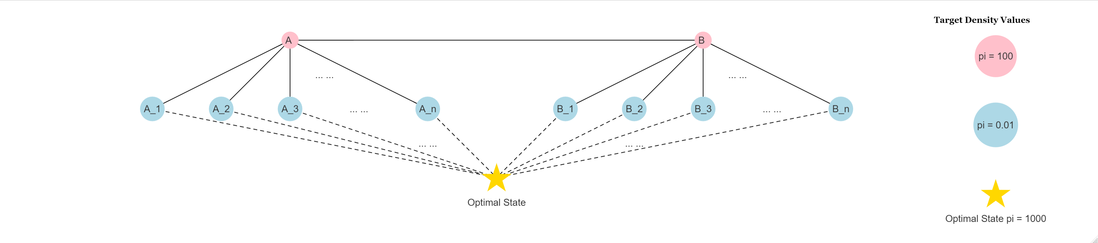
Although the Rejection-Free algorithm for optimization can help reduce the inefficiency of rejections, local maximum areas of $\pi$ can still be a problem. For example, we want to find $X\in S$, which maximizes $\pi(X)$ from a state space starting at state $A$ in Figure 1. Here, we use a uniform proposal distribution $\mathcal{Q}$ on the neighbor sets $\mathcal{N}$ as shown in Figure 1. We will have many rejections if we constantly use Simulated Annealing with $T\equiv 1$. Note that, $\pi(A_{1})=\pi(A_{2})=\dots=\pi(A_{n})=0.01$ while $\pi(A)=\pi(B)=100$. The probability of escaping from A is $\frac{1}{n+1}+\frac{n}{n+1}\times\frac{1}{10000}$, where $\frac{1}{n+1}$ represents the probability of moving from state A to state B, and $\frac{n}{n+1}\times\frac{1}{10000}$ is the probability of moving from state A to $A_{1},A_{2},\dots,A_{n}$. Cooling Schedules can help reduce the probability of rejection at the beginning of Simulated Annealing since $T$ should be large at the beginning. However, as we move on in Simulated Annealing, we will be more and more likely to be trapped by local maximum areas like this. The Rejection-Free algorithm for optimization can produce some speedup in this case, but the Rejection-Free chain will still be stuck by the local maximum area $\{\pi(A),\pi(B)\}$. If $n$, the number of other neighbors for $A$ and $B$, is small, this chain will be switching between A and B for a really long time, since

To help our Markov chain escape from those local maximums in optimization, we propose another method called Partial Neighbor Search based on the Rejection-Free algorithm.

Partial Neighbor Search (PNS) is an algorithm based on the Rejection-Free, also designed as a Markov chain used for optimization as described in Algorithm 5. Algorithm 5 is again designed to converge to states $X_{k}$ with nearly-maximal values of $\pi(X_{k})$, with greater efficiency by avoiding both rejections and traps in local maximum areas.

The $(\star)$ step in Algorithm 5 is the key of PNS. At this step, $\mathcal{N}_{k}(J_{k-1})$ could be random $50\%$ of the elements from $\mathcal{N}(J_{k-1})$. In Section 6, we will explore many other choices for the $(\star)$ step to figuring out the best strategy. Moreover, for continuous cases, PNS can be applied, and we only need to ensure the Partial Neighbor Sets $\mathcal{N}_{k}$ are always finite, $\forall k$. On the other hand, Algorithms 3 and Algorithm 4 for Rejection-Free only work for discrete cases where the number of neighbors for all states must be finite, and we will illustrate these by an optimization example in continuous cases in Section 10.

The motivation for PNS is simple: we have a better chance of escaping from the local maximum area if we force the algorithm to avoid some neighbors randomly. For example, in Figure 1, if we only consider half of the neighbors at state $A$, then we may disregard state $B$ with probability $50\%$, then we have a probability of at least $50\%$ of selecting a state from $\{A_{1},A_{2},\dots,A_{n}\}$ as our next state in the PNS chain. If this occurs, we are more likely to escape from the local maximum area $\{\pi(A),\pi(B)\}$.

The quadratic unconstrained binary optimization (QUBO) has gained increasing attention in the field of combinatorial optimization due to its wide range of applications in finance and economics to machine learning (Kochenberger et al 2014). The QUBO problem is known to be NP-hard (Glover et al 2018), so it is common to use Simulated Annealing to find the optimal or workable solution. This problem can now be addressed using our PNS algorithm. (Additional applications are in Sections 8, Section 9, and Section 10 below.)

For a given $N$ by $N$ matrix $Q$ (usually upper triangular), the QUBO question aims to find

(Sometimes $\arg\min$ is used in place of $\arg\max$, which is equivalent to taking the negative of $Q$, so for simplicity, we focus on the $\arg\max$ version here.)

As part of our algorithm, we use a uniform proposal distribution among all neighbors where the neighbors are defined as binary vectors with Hamming distance 1. That is, $\mathcal{Q}(X,Y)=\frac{1}{N}$ for $\forall Y\in\mathcal{N}(X)$, where $Y\in\mathcal{N}(X)\iff\lvert X-Y\rvert=\sum_{i=1}^{N}\lvert X_{i}-Y_{i}\rvert=1$, $\forall X,Y\in\{0,1\}^{N}$. We randomly choose half of the neighbors at each step of PNS, which means we only consider a random subset $\mathcal{N}_{K}(x)\subset\mathcal{N}(x)$ whose cardinality is $\lvert\mathcal{N}_{k}(X)\rvert=\frac{1}{2}\lvert\mathcal{N}(X)\rvert=\frac{1}{2}N$ for $\forall X\in\{0,1\}^{N}$. In addition, the target distribution $\pi(x)=\exp\{x^{T}Qx\}$, since we need the target distribution to be positive all time to use the Cooling Schedule, and maximizing $x^{T}Qx$ is the same as maximizing $\exp\{x^{T}Qx\}$. Furthermore, $T(k)$ represents the temperature at step $k$ for the cooling schedule here.

We compare Simulated Annealing, Rejection-Free for Optimization, and PNS in 1000 simulation runs. We randomly generate a 200 by 200 upper triangular as the QUBO matrix $Q$. The non-zero elements from $Q$ were generated randomly by $Q_{i,j}\sim\text{Normal}(0,100^{2})\mbox{, }\forall i\leq j$.

The result for the simulation is shown in Figure 2. Here, we used a violin plot to summarize the results. The violin plot uses the information available from local density estimates and the basic summary statistics to provide a useful tool for data analysis and exploration (Hintze and Nelson 1998). The violin plot combines two density traces on both sides and three quantile lines ($25\%$, $50\%$, and $75\%$) to reveal the data structure. In addition, we added a long segment of the bottom layer as the mean for the values. We also added a short segment on the y-axis to help compare the mean values.

From Figure 2, we can see that the PNS is always the best in all four different cooling schedules. Note that the number of iterations used for Simulated Annealing is $200,000$ for Simulated Annealing while they are $1000$ for both Rejection-Free and PNS. We used these many iterations because we need to consider $200$ neighbors at each iteration in Rejection-Free, while we only need to consider one neighbor for each iteration in Simulated Annealing. If we proceed with all three algorithms on a single-core machine, the run time of a single simulation run for simulated Annealing is about 20 seconds; the run time for Rejection-Free is about 10 seconds; the run time for PNS is only 5 seconds. In addition, parallelism in computer hardware can increase the speed of both Rejection-Free and PNS by distributing the calculation of the transition probabilities for different neighbors onto different cores (Rosenthal et al 2021). Besides that, we can also use multiple replicas at different temperatures, such as in parallel tempering, or deploy a population of replicas at the same temperature (Sheikholeslami 2021). Combining these methods by parallelism can yield 100x to 10,000x speedups for both Rejection-Free and PNS (Sheikholeslami 2021).

In the above example, the improvement in the efficiency of Rejection-Free is not hard to understand. The performance of PNS is somehow counter-intuitive. Compared to Rejection-Free, why would we get a better result by considering fewer neighbors at each step? To illustrate how PNS works, we can look closely at the Markov chains generated in the above example.

In this section, we found a local maximum area for the target distribution $\pi$ purposefully in the previous QUBO example in Section 4 by looking at the final results from the simulation runs from the previous section. Many Rejection-Free chains stopped at this local maximum area after 1000 iterations. For this local maximum area, the target distribution value is around 82600, and this local maximum area contains three states whose target distribution values are much larger than all their other neighbors. Thus, this local maximum can trap the regular Rejection-Free chain for a long time, just like the cases we mentioned in Figure 1. We can plot the Markov chains by PNS with the target distribution values for all the neighbors by Rejection-Free and the random subset of neighbors by PNS in the form of boxplots. The boxplot of the first 30 steps from the first simulation in PNS is shown in the first plot in Figure 3

From the first plot in Figure 3, most of the target distribution values within the boxplot are not useful since they are too small to be picked by the algorithm. Therefore, we only need to consider the important neighbors likely to be chosen. Firstly, for each state $J_{k}$ in the Markov Chain, we find the max value among all the transition probabilities, and we define the important neighbors to be those neighbors whose transition probability is larger than $\exp\{-10\}$ times the highest transition probability among all neighbors. That is, for each $J_{k}$ from the chain, we find $q(Y_{0})=\max\{q(Y)\mid Y\in\mathcal{N}(J_{k})\}$, and then we define $\{Y\mid Y\in\mathcal{N}(J_{k}),q(Y)>\exp\{-10\}\times q(Y_{0})\}$ to be important neighbors for $J_{k}$. This time, we only have several important neighbors at each step. Thus, we used points instead of boxplots to show the important neighbors. The result from Rejection-Free and PNS is also shown in Figure 3.

From the second plot in Figure 3, the red dots represent the important neighbors, and the pink line means the Rejection-Free chain. We can see that this local maximum area of three states can easily trap the Rejection-Free chains because their target distribution values are much higher than all other neighbors. Thus, the important neighbors for any of these three states are only the remaining two, and the Rejection-Free chain will be switching between these three for a long time. At the same time, the blue dots in the second plot represent the important neighbors if we start to do PNS from that state. Although we did not apply PNS in the second plot, we still put the random subset for PNS there as a comparison. From the blue dots in the second plot, we can say that if we perform PNS, then the Markov chain can escape from this local maximum area faster since some groups of the blue dots do not contain any of these three states with high target distribution values.

On the other hand, the third plot in Figure 3 shows that the PNS chain (blue line) escapes from this local maximum area within five steps. Again, the blue dots represent the important neighbor from PNS, and the red dots represent the important neighbor if we start to perform Rejection-Free from that step. For each step of PNS within the local maximum area of three states, the Markov Chain has the probability of $25\%$ to include neither of the remaining neighbors from the three states. Thus, PNS helped the Markov chain to escape from this local maximum area. In addition, in the middle part of the PNS chain, when the target distribution value of the PNS chain is increasing, we usually have more than one important neighbor. For example, if we have three important neighbors, we only have $12.5\%$ for considering none of them by PNS.

Thus, the PNS is better than Rejection-Free because the PNS performs much better than the Rejection-Free algorithm when the local maximum areas trap the Markov chain. On the other hand, PNS is not much worse than Rejection-Free when the Markov chain is increasing with respect to the target distribution value.

This section uses $50\%$ random partial neighbors for each step. We have many other choices, and we will consider and compare these choices in the next section.

We formally define the way of choosing Partial Neighbors Sets. Before we start the Markov chain, we need to define a proposal distribution $\mathcal{Q}$ and corresponding neighbor sets $\mathcal{N}(X):=\{Y\in S\mid\mathcal{Q}(X,Y)>0\}$. Partial Neighbor Sets $\mathcal{N}_{k}$ means any set satisfies the following conditions:

1. 1.

   $\mathcal{N}_{k}:\mathcal{S}\to P(\mathcal{S})$, where $\mathcal{S}$ is the state space, and $P(\mathcal{S})$ is the power set of $\mathcal{S}$.

2. 2.

   $\mathcal{N}_{k}(X)\subset\mathcal{N}(X)$, $\forall X\in\mathcal{S}$.

3. 3.

   $Y\in\mathcal{N}_{k}(X)\iff X\in\mathcal{N}_{k}(Y)$, $\forall X,Y\in\mathcal{S}$.

4. 4.

   Define $\mathcal{Q}_{k}(X,Y):\mathcal{S}\times\mathcal{S}\to\mathbb{R}$ be the corresponding partial proposal distribution where $\mathcal{Q}_{k}(X,Y)\propto\mathcal{Q}(X,Y)$ for $Y\in\mathcal{N}_{k}(X)$ and $\mathcal{Q}_{k}(X,Y)=0$ otherwise.

5. 5.

   Define the Partial Neighbor Weight $t\coloneqq\int_{Y\in\mathcal{N}_{k}(X)}\mathcal{Q}(X,y)dy$. Note that if we want to ensure the reversibility of the Markov chain, then we have to make sure the Partial Neighbor Weight is a constant.

Usually, we want to pick $\mathcal{N}_{i}$ such that $\lvert\mathcal{N}_{k}(X)\rvert<\lvert\mathcal{N}(X)\rvert$ to perform proper PNS. In addition, to ensure irreducibility, we need to make sure $\cup_{i=0}^{K-1}\mathcal{N}_{k}(X)=\mathcal{N}(X)$ for all $X\in\mathcal{S}$.

Here, we compare the four different ways to choose the proposal distribution $\{\mathcal{Q}_{k},\mathcal{N}_{k}\}$ for PNS in the $(\star)$ step in Algorithm 5:

• •

  Method A (random subset every step): The Partial Neighbor Sets $\mathcal{N}_{k}$ are randomized for every step, where $\lvert\mathcal{N}_{k}(X)\rvert=\frac{1}{2}\times\lvert\mathcal{N}(X)\rvert$. $\mathcal{Q}_{k}$’s are defined accordingly.

• •

  Method B (random subset every 10 steps): The Partial Neighbor Sets $\mathcal{N}_{k}$ are randomized for once 10 steps, where $\lvert\mathcal{N}_{k}(X)\rvert=\frac{1}{2}\times\lvert\mathcal{N}(X)\rvert$. That is, $\mathcal{N}_{10\times k+1}=\mathcal{N}_{10\times k+2}=\dots=\mathcal{N}_{10\times k+10}$ for $\forall k\in\mathbb{N}$. $\mathcal{Q}_{k}$’s are defined accordingly.

• •

  Method C (systematic subset every step): Before we start our Markov Chain, we define two Partial Neighbor Sets $\mathcal{N}_{1}$ and $\mathcal{N}_{2}$, where $\lvert\mathcal{N}_{1}(X)\rvert=\lvert\mathcal{N}_{2}(X)\rvert=\frac{1}{2}\times\lvert\mathcal{N}(X)\rvert$, $\mathcal{N}_{1}(X)\cap\mathcal{N}_{2}(X)=\emptyset$. For step $k$ of the Markov chain, we only randomly generate $r_{k}\in\{1,2\}$, and apply $\mathcal{N}_{r_{k}}$ for step $k$. $\mathcal{Q}_{1}$ and $\mathcal{Q}_{2}$ are defined accordingly.

• •

  Method D (systematic subset every 10 steps): Before we start our Markov Chain, we define two Partial Neighbor Sets $\mathcal{N}_{1}$ and $\mathcal{N}_{2}$, where $\lvert\mathcal{N}_{1}(X)\rvert=\lvert\mathcal{N}_{2}(X)\rvert=\frac{1}{2}\times\lvert\mathcal{N}(X)\rvert$, $\mathcal{N}_{1}(X)\cap\mathcal{N}_{2}(X)=\emptyset$. For every ten steps of the Markov chain, we only randomly generate $r_{k}\in\{1,2\}$ and apply $\mathcal{N}_{r_{k}}$. That is $r_{10\times k+1}=r_{10\times k+2}=\ldots=r_{10\times k+10}$ for $\forall k\in\mathbb{N}$. $\mathcal{Q}_{1}$ and $\mathcal{Q}_{2}$ are defined accordingly.

Again, we use the $200\times 200$ QUBO example. The settings for the simulation are the same as in Section 4. For Method C and D, the two Partial Neighbor Sets $\mathcal{N}_{1}$ and $\mathcal{N}_{2}$ are defined to be flipping the first 100 entries in $x$ and flipping the last 100 entries in $x$. The result for the simulation is shown in Figure 4. This figure shows that the random subset at every step (Method A) performs the best in all four Cooling Schedules. Therefore, we will keep using Method A in all later parts.

In addition, we used Partial Neighbor Sets with half elements from all neighbors in previous simulations. Now we compare the Partial Neighbor Sets with cardinality of $\lvert\mathcal{N}(X)\rvert\times\{1,\frac{3}{4},\frac{2}{3},\frac{1}{2},\frac{1}{3},\frac{1}{4},\frac{1}{5},\frac{1}{6},\frac{1}{7},\frac{1}{8}\}$ by the same simulation settings as before. From Figure 5, we can see that $\frac{1}{3},\frac{1}{4},\frac{1}{5}$ are overall the best among all the choices. Thus, we can conclude that Partial Neighbor Sets with around $25\%$ of the neighbors being considered at each step are the best for the QUBO question stated above.

Therefore, we conclude that our best method to do optimization for the $200\times 200$ QUBO question is Algorithm 6.

Tabu search (Glover 1989) (Glover 1990) is also a methodology in optimization that guides a local heuristic search procedure to explore the solution space beyond local optimality. The idea of Tabu search is to prohibit access to specific previously-visited solutions. Tabu search is the most intuitive method to help the Markov Chain escape from local maximum areas, as in Figure 1. After moving from state A to state B, we must choose our next state among $\{B_{1},B_{2},\dots,B_{N}\}$. We can combine our Rejection-Free algorithm for optimization with Tabu search and then compare this new method to the PNS by the QUBO question. Note that we do not need to record all visited states since we are almost impossible to revisit a state after a certain number of steps. Thus, we only need to record the last several steps and prohibit our Markov chain from revisiting them. The new algorithm is formulated as Algorithm 7.

Here, we compare PNS with L-step Simplified Tabu Rejection-Free for $L=1,2,3,\dots,9$. Again, we randomly generate a 200 by 200 upper triangular QUBO matrix. The non-zero elements from the 200 by 200 upper triangular matrix $Q$ were generated randomly with $Q_{i,j}\sim N(0,100^{2})$ for $i<j$. Note that we need to consider about $200$ neighbors at each step for both Rejection-Free and Simplified Tabu Rejection-Free, while we only need to consider $50$ neighbors at each iteration for PNS. If we proceed with the algorithms with a single-core implementation, Rejection-Free and Tabu Rejection-Free need about four times longer than PNS with the same number of steps. Therefore, we can compare the PNS with $4\times 100=400$ iterations with the other methods to get a fair comparison for the program on a single core. Note that we are using this many numbers of steps here because 400 steps are enough for PNS to find a good enough answer. The result for the simulation is shown in Figure 6. From this plot, we can see that PNS performs much better than Rejection-Free and Simplified Tabu Rejection-Free.

The Knapsack problem is another well-known NP-hard problem in optimization (Salkin and De Kluyver 1975). We consider the simplest 0-1 Knapsack problem here. Given a knapsack of max capacity $W$ and $N$ items with corresponding values $\{v_{i}\}_{i=1}^{N}$ and weights $\{w_{i}\}_{i=1}^{N}$, we want to find a finite number of items among all $N$ items which can maximize the total value while not exceeding the max capacity of the knapsack. That is, for given $W>0$, $\{v_{i}\}_{i=1}^{N}>0$ and $\{w_{i}\}_{i=1}^{N}>0$, find a sequence of $N$ binary variable $\{X_{i}\}_{i=1}^{N}\in\{0,1\}$ to maximize

Since the Knapsack problem is NP-hard, we can use the Simulated Annealing algorithm to find a feasible solution. For this simulation, we set $W=100,000$. We randomly generate $N=1000$ items where the values and weights are random by $w_{i},v_{i}\sim\mbox{Poisson}(1000)$. The mean and the variance for $\mbox{Poisson}(1000)$ are both 1000. Suppose we want to find a binary vector $X=(X_{1},X_{2},\dots,X_{N})^{T}$ of dimension $N$ to maximize $v^{T}X$ subject to $w^{T}X\leq W$.

Again, we used a uniform proposal distribution among all neighbors where the neighbors are defined as binary vectors with Hamming distance 1. That is, $\mathcal{Q}(X,Y)=\frac{1}{N}$ for $\forall Y\in\mathcal{N}(X)$, where $Y\in\mathcal{N}(X)\iff\lvert X-Y\rvert=\sum_{i=1}^{N}\lvert X_{i}-Y_{i}\rvert=1$, $\forall X,Y\in\{0,1\}^{N}$. We randomly choose half of the neighbors at each step for PNS. That is, $\lvert\mathcal{N}_{k}(X)\rvert=\frac{1}{2}\lvert\mathcal{N}(X)\rvert=500$ for $\forall X\in\{0,1\}^{N}$. Moreover, the target density $\pi(X)=\mathbb{1}(w^{T}X\leq W)\times v^{T}X$, where $\mathbb{1}$ represents the indicator function. In addition, $T(k)$ represents the temperature at step $k$ for the Cooling Schedule here.

Again, we compare Simulated Annealing, Rejection-Free with PNS here. The result is shown in Figure 7. The plot shows that Rejection-Free for optimization and PNS algorithm are better than the regular Simulated Annealing algorithm in all four Cooling Schedules. Again, for the simulation shown in Figure 7, the numbers of iterations used for the three methods are set to be different to have a fair comparison between three methods. We set the number of iterations for Simulated Annealing to be $1000,000$. The numbers of iterations for Rejection-Free and PNS are $1000$ since we need to consider $1000$ neighbors at each iteration for Rejection-Free for optimization. In contrast, we only need to consider one neighbor for each iteration in Simulated Annealing.

This result shows that PNS is not always that much better than Rejection-Free when the number of iterations is the same. In some cases, where the target distribution is not sharply peaked, and there are not too many local extreme areas, Rejection-Free can also have excellent performance. Note that if we run the above simulation on a single core, PNS will only take about half of the time used by Rejection-Free, and if we use parallel hardware to apply the above algorithm, Rejection-Free and PNS will take about the same time.

In addition, Rejection-Free is not always better than simple Simulated Annealing. For example, if $\pi(X)\equiv 1$ for all $X\in S$, there will be no rejections. The Simulated Annealing will move to a new state by computing a single probability, while the Rejection-Free will do the same but compute the probabilities for all neighbors. However, when the dimension of the problem is large, or the target density is sharply peaked, the PNS will perform much better than Rejection-Free, and Rejection-Free will perform much better than Simulated Annealing.

The 3R3XOR problem is a methodology for generating benchmark problem sets for Ising machines devices designed to solve discrete optimization problems cast as Ising models introduced by Hen 2019. The Ising model, named after Ernst Ising, is concerned with the physics of magnetic-driven phase transitions (Cipra 1987). The Ising model is defined on a lattice, where a spin $s_{i}\in\{-1,1\}$ is located on each lattice site (Block and Preis 2012). The optimization question for the Ising model has been widely applied to many scientific problems such as neuroscience (Hopfield 1982) and environmental science (Ma et al 2014). Thus, algorithms, even special-purpose programmable devices, designed to solve discrete optimization problems cast as Ising models are popular (Hen 2019), and our PNS algorithm is one of them.

However, the non-planar Ising model is NP-complete (Cipra 2000). We cannot find an optimal state from an Ising model in polynomial time. Then, it is hard for us to compare the performance of the heuristic solvers, such as Rejection and PNS, by the time used to find the optimal state from a random Ising model. On the other hand, Hen 2019 introduced a tool for benchmarking Ising machines in 2019. In his approach, linear systems of equations are cast as Ising cost functions. The linear systems can be solved quickly, while the corresponding Ising model exhibits the features of NP-hardness (Hen 2019). This way, we can construct special Ising models with a unique known optimal state. Then we can use these special Ising models to compare the heuristic solvers’ runtimes for finding the optimal state.

In this section, we focus on constructing a simplified version of 3-body Ising with $N$ spins from a binary linear system of $N$ equations. The simplified version is defined as follows:

where $s_{i}\in\{-1,1\}$ for $\forall i=1,2,\ldots,N$. $\mathbf{M}_{a,b,c}$ is a $N\times N\times N$ matrix where $\mathbf{M}_{a,b,c}=0$ $\forall a\geq b$, $b\geq c$, or $a\geq c$.

In Hen 2019’s (Hen 2019) approach, we start by choosing a binary matrix $\{\mathbf{A}_{i,j}\}$ and a binary vector $\{\mathbf{b}_{j}\}$ to form a modulo 2 linear system of N equations in N variables.

This module 2 linear system of equations can always be solved in polynomial time using Gaussian elimination. In addition, as long as the binary matrix $\{\mathbf{A}_{i,j}\}$ is invertible, the solution (if exists) is unique. Suppose $\{x_{1},...,x_{n}\}$ are $n$ binary variables. Then for given $\{\mathbf{A}_{i,j}\}$ and $\{\mathbf{b}_{j}\}$, we define

where $\mathbb{1}$ means indicator function here. Since $F$ is a sum of $N$ indicator functions, then $0\leq F\leq N$ and the minimum bound is reached when $\{x_{j}\}$ is the solution to the modulo 2 linear system.

Let $s_{j}=1-2x_{j}\in\{-1,1\}\mbox{ for }j=1,2,\dots,N$ be $N$ Ising spins. Then we must have

$\forall i=1,2,\dots,m$. Then

After dropping immaterial constants, we define

Note that $F\geq 0$ and the minimum bound is reached when $\{x_{j}\}$ is the solution to the modulo 2 linear system. Thus, $F_{0}\leq N$, and the maximum bound will be reached when $\{x_{j}\mid x_{j}=\frac{1}{2}(1-s_{j})\}$ is the solution to the modulo 2 linear system. In addition, as long as the matrix $\{\mathbf{A}_{i,j}\}$ is invertible, the solution to the equation system must uniquely exist, and then there must exist a single configuration maximize $F_{0}$ whose maximum value is exactly $N$.

Again, the Hamiltonian for simplified 3-body Ising model including only the cubic term to be $H(\{s_{j}\})=\sum_{a<b<c}\mathbf{M}_{a,b,c}s_{a}s_{b}s_{c}$. Here, we assume, on each row of binary matrix $\{\mathbf{A}_{i,j}\}$, $\sum_{j=1}^{N}\mathbf{A}_{i,j}=3$. Then, let $\mathbf{M}_{a,b,c}=(-1)^{\mathbf{b}_{i}}$ if $\exists i,a<b<c$ such that $\mathbf{A}_{i,a}=\mathbf{A}_{i,b}=\mathbf{A}_{i,c}=1$, and $\mathbf{M}_{a,b,c}=0$ otherwise. Then, we have $H(\{s_{j}\})=F_{0}(\{s_{j}\})$.

Thus, we can construct an Ising model with a unique optimal bound with a known optimal value $N$ as follows:

1. 1.

   find an invertible binary matrix $\{\mathbf{A}_{i,j}\}$ and a binary vector $\{\mathbf{b}_{i}\}$, where $\sum_{j=1}^{N}\mathbf{A}_{i,j}=3$, $\forall i$

2. 2.

   solve the modulo 2 linear equation system $\sum_{j=1}^{N}\mathbf{A}_{i,j}x_{j}\equiv\mathbf{b}_{i}\mod 2$, for $i=1,2,\dots,N$ to make sure the unique solution exists

3. 3.

   define $\mathbf{M}_{a,b,c}$ be a $N\times N\times N$ matrix where $\mathbf{M}_{a,b,c}=(-1)^{\mathbf{b}_{i}}$ if $\exists i,a<b<c$ such that $\mathbf{A}_{i,a}=\mathbf{A}_{i,b}=\mathbf{A}_{i,c}=1$, and $\mathbf{M}_{a,b,c}=0$ otherwise

4. 4.

   then we must have a unique optimal solution $s_{\max}$ for $H(s_{\max})=\max(H(s))=N$

By constructing the special 3-body $N\times N\times N$ Ising model with a unique optimal solution of maximum bound $N$, we can examine the performance of the Rejection-Free and PNS algorithms on these special Ising models. Again, uniform proposal distributions are used here, and the neighbors are defined as binary vectors with Hamming distance 1. We random generate the special Ising models with four different sizes $N=12$, $24$, $48$ and $96$. For each of these four different sizes, we generate 50 different Ising models and record the time used by the algorithms to reach the unique optimal state. The median of these 50 results for both Rejection-Free and PNS algorithms are shown in Figure 8. From this figure, Rejection-Free is the worst. $25\%$ PNS performs comparably to $75\%$, and the $50\%$ PNS performs the best.

In previous sections, we focused on optimization questions with the discrete state space $\mathcal{S}$ where all states have at most a finite number of neighbors. Meanwhile, Simulated Annealing works for general state space. In addition, Theorem $13$ in Rosenthal et al 2021 extended the Rejection-Free for sampling to general state space. Similarly, we can extend the Rejection-Free for optimization to general state space.

Although we have a solid theory base for Rejection-Free in general state space, it is challenging to apply Rejection-Free to those cases. There is a major difficulty involved in the for loop that calculates the transition probability of all neighbors in Algorithm 4. In continuous cases, although numerical integration of all transition probability can be performed, it is unlikely that such tasks may be efficiently divided among specialized hardware with a certain number of parallel processing units. On the other hand, PNS, as described in Algorithm 5, can be applied straightforwardly to continuous cases by choosing the Partial Neighbors Sets $\mathcal{N}_{k}(X)$ to be finite subsets of all the neighbors $\mathcal{N}(X)$ in Algorithm 5.

We compare the performance of Simulated Annealing with our PNS on a simple example of quadratic programming, which belongs to the category of continuous optimization, as stated below:

where $Q$ is a given an upper triangular $N$ by $N$ matrix and $x\in\mathbb{R}^{N}$. For most cases, the quadratic programming is stated by $\arg\min$ instead of $\arg\max$. We use the $\arg\max$ version here to be consistent with the QUBO question in Section 4, and $\arg\max$ is equivalent to $\arg\min$ when replacing $Q$ by $-Q$. This quadratic programming question is also NP-hard as long as $Q$ is indefinite (Sahni 1974), where indefinite means matrices that are neither positive semi-definite nor negative semi-definite.

We randomly generate a 200 by 200 upper triangular to be the matrix $Q$, where the non-zero elements from the 200 by 200 upper triangular matrix $Q$ were generated randomly by $Q_{i,j}\sim\text{Normal}(0,100^{2})\mbox{, }\forall i\leq j$. We compare Simulated Annealing and PNS in 100 simulation runs here. We omit Rejection-Free since applying Rejection-Free to continuous cases is quite hard.

The target density value is set to be $\pi(x)=\exp\{x^{T}Qx\}$, $\forall x$ such that $x_{i}\in(0,1)$, $\forall i=1,2,\dots,N$, and $\pi(x)=-\infty$ otherwise. In addition, the proposal distribution $\mathcal{Q}$ and the corresponding neighbor set $\mathcal{N}$ are defined as follows:

1. 1.

   for state $x=(x_{1},x_{2},\dots,x_{N})^{T}\in\mathcal{S}$, choose a random entry $x_{r}$ for $r\in\{1,2,\dots,N\}$;

2. 2.

   generate a random value $s\sim\text{Normal}(0,0.1^{2})$;

3. 3.

   let $y_{r}=x_{r}+s$ and $y_{n}=x_{n}\times\frac{1-x_{r}}{1-y_{r}}$, $\forall n\neq r$;

4. 4.

   if $y_{r}\notin(0,1)$, then the corresponding $\pi(y)$ is defined to be $-\infty$; in practice, we just need to generate a new $y$; also note that, as long as $y_{r},x\in(0,1)$, we must have $y\in(0,1)$ as well;

5. 5.

   to ensure the reversibility within each Partial Neighbor Set, we also consider $y^{\prime}_{r}=x_{r}-s$ and $y^{\prime}_{n}=x_{n}\times\frac{1-x_{r}}{1-y^{\prime}_{r}}$, $\forall n\neq r$; if $y^{\prime}_{r}\notin(0,1)$, then we can ignore $y^{\prime}$.

With the given steps, we have $\sum_{n=1}^{N}y_{n}=1$ as long as $\sum_{n=1}^{N}x_{n}=1$. This method is similar to component-wise Simulated Annealing. We find a random component, magnify or minify it, and then modify the rest of the entries accordingly to make the summation remain unchanged. This proposal distribution $\mathcal{Q}$ is therefore systematic. By the above ways to generate neighbors, we can eliminate the constraints that $x_{i}\geq 0\mbox{, }\forall i=1,2,\dots,N$, and $\sum_{i=1}^{N}x_{i}=1$, and we only need to focus on $\arg\max x^{T}Qx$.

For Simulated Annealing, we randomly generate one neighbor by the above given steps and calculate the transition probability. For PNS, we can generate, for example, $20$ random neighbors at each step. In this case, the Partial Neighbor Set $\mathcal{N}_{i}$ is only a random subset of $\mathcal{N}$ with $20$ elements, and thus, the implementation of PNS is simple compared to the Rejection-Free.

The result for the simulation is shown in Figure 9. We can see that the PNS performs better than Simulated Annealing in all four different cooling schedules. However, the difference between PNS and Simulated Annealing in this continuous example is not as much as the difference between the algorithms from the discrete QUBO questions. This is because the continuous example is not as sharply peaked as the discrete example from Section 6. After we choose a random entry $r$, we only need to move a small step around the original value of $x_{r}$. On the other hand, we have to flip between $0$ and $1$ in the discrete example. Thus, the rejection rate for the Simulated Annealing is lower than the rate from the discrete example, so the performance of these two algorithms gets closer.

In addition, PNS is specially designed for parallelism hardware. Again, with a specialized dedicated processor such as DAU, PNS can yield 100x to 10,000x speedups Sheikholeslami 2021. In addition, this example also shows PNS has more flexibility compared to the Rejection-Free algorithm. Again, Rejection-Free can hardly work for cases with infinite neighbors, while PNS can be easily applied by choosing finite $\mathcal{N}_{k}$.

Moreover, the number of elements in $\mathcal{N}_{k}$ needs to be reasonable for PNS to keep its performance. For example, if we used $\lvert\mathcal{N}_{k}\rvert=500$, we would calculate too many transition probabilities at each step, and the algorithm would be inefficient. Meanwhile, if we used $\lvert\mathcal{N}_{k}\rvert=2$, the number of Partial Neighbor Sets being considered at each step would be too few. As PNS will force the Markov chain to move to one element from the Partial Neighbor Set $\mathcal{N}_{k}$, it will move to some terrible choices of states when all states in the Partial Neighbor Set $\mathcal{N}_{k}$ have small target distribution values. In the above simulation, choosing $\lvert\mathcal{N}_{k}\rvert$ from $10$ to $30$ won’t make a big difference.

This paper illustrates Rejection-Free Simulated Annealing algorithms that consider all neighbors at each step in order to prevent inefficiency from rejections. We have also proposed a Partial Neighbor Search (PNS) algorithm based on the Rejection-Free technique in order to address the issue of local maximum area. Three sets of discrete examples have been simulated to demonstrate that PNS can produce significant speedups in optimization problems. PNS has also been applied to continuous examples in order to demonstrate its greater flexibility in comparison to Rejection-Free.

The author(s) would like to thank Fujitsu Ltd. and Fujitsu Consulting (Canada) Inc. for providing financial support.

References

- Albright (2007) Albright B (2007) An introduction to simulated annealing. The College Mathematics Journal 38(1):37–42.
- Beichl and Sullivan (2000) Beichl I, Sullivan F (2000) The Metropolis algorithm. Computing in Science & Engineering 2(1):65–69.
- Bertsimas and Tsitsiklis (1993) Bertsimas D, Tsitsiklis J (1993) Simulated annealing. Statistical science 8(1):10–15.
- Bianchi et al (2009) Bianchi L, Dorigo M, Gambardella LM, et al (2009) A survey on metaheuristics for stochastic combinatorial optimization. Natural Computing 8(2):239–287.
- Block and Preis (2012) Block B, Preis T (2012) Computer simulations of the Ising model on graphics processing units. The European Physical Journal Special Topics 210(1):133–145.
- Cipra (1987) Cipra BA (1987) An introduction to the Ising model. The American Mathematical Monthly 94(10):937–959.
- Cipra (2000) Cipra BA (2000) The Ising model is NP-complete. SIAM News 33(6):1–3.
- Floudas and Pardalos (2008) Floudas CA, Pardalos PM (2008) Encyclopedia of optimization, Springer Science & Business Media, pp 1538–1542.
- Garey et al (1974) Garey MR, Johnson DS, Stockmeyer L (1974) Some simplified NP-complete problems. In: Proceedings of the sixth annual ACM symposium on Theory of computing, pp 47–63.
- Glover (1989) Glover F (1989) Tabu search—part I. ORSA Journal on computing 1(3):190–206.
- Glover (1990) Glover F (1990) Tabu search—part II. ORSA Journal on computing 2(1):4–32.
- Glover et al (2018) Glover F, Kochenberger G, Du Y (2018) A tutorial on formulating and using QUBO models. arXiv:1811.11538
- Hen (2019) Hen I (2019) Equation planting: A tool for benchmarking Ising machines. Phys Rev Applied 12:011,003.
- Hintze and Nelson (1998) Hintze JL, Nelson RD (1998) Violin plots: a box plot-density trace synergism. The American Statistician 52(2):181–184.
- Hitchcock (2003) Hitchcock DB (2003) A history of the Metropolis-Hastings algorithm. The American Statistician 57(4):254–257.
- Hopfield (1982) Hopfield JJ (1982) Neural networks and physical systems with emergent collective computational abilities. Proceedings of the national academy of sciences 79(8):2554–2558.
- Kirkpatrick et al (1983) Kirkpatrick S, Gelatt CD, Vecchi MP (1983) Optimization by simulated annealing. science 220(4598):671–680.
- Kochenberger et al (2014) Kochenberger G, Hao JK, Glover F, et al (2014) The unconstrained binary quadratic programming problem: a survey. Journal of combinatorial optimization 28(1):58–81.
- Ma et al (2014) Ma YP, Sudakov I, Strong C, et al (2014) Ising model for melt ponds on Arctic sea ice. arXiv:1408.2487
- Matsubara et al (2020) Matsubara S, Takatsu M, Miyazawa T, et al (2020) Digital annealer for high-speed solving of combinatorial optimization problems and its applications. 2020 25th Asia and South Pacific Design Automation Conference (ASP-DAC) pp 667–672.
- Metropolis et al (1953) Metropolis N, Rosenbluth AW, Rosenbluth MN, et al (1953) Equation of State Calculations by Fast Computing Machines. The Journal of Chemical Physics 21(6):1087–1092.
- Rosenthal et al (2021) Rosenthal JS, Dote A, Dabiri K, et al (2021) Jump Markov chains and rejection-free Metropolis algorithms. Computational Statistics 36(4):2789–2811.
- Rutenbar (1989) Rutenbar RA (1989) Simulated annealing algorithms: An overview. IEEE Circuits and Devices magazine 5(1):19–26.
- Sahni (1974) Sahni S (1974) Computationally related problems. SIAM Journal on computing 3(4):262–279.
- Salkin and De Kluyver (1975) Salkin HM, De Kluyver CA (1975) The knapsack problem: a survey. Naval Research Logistics Quarterly 22(1):127–144.
- Schrijver (2005) Schrijver A (2005) On the history of combinatorial optimization (till 1960). Handbooks in operations research and management science 12:1–68.
- Sheikholeslami (2021) Sheikholeslami A (2021) The power of parallelism in stochastic search for global optimum: Keynote paper. In: ESSCIRC 2021 - IEEE 47th European Solid State Circuits Conference (ESSCIRC), pp 36–42.
- Sodan et al (2010) Sodan AC, Machina J, Deshmeh A, et al (2010) Parallelism via multithreaded and multicore CPUs. Computer 43(3):24–32