A Simple Nonconforming Tetrahedral Element for the Stokes Equations

We consider the Stokes equations in a domain $\Omega$ in ${\mathbb{R}}^{3}$: find the velocity ${\boldsymbol{u}}=\left[u_{i}\right]_{i=1}^{3}$ and the pressure $p$ such that

Let us define the spaces

and

where $(\cdot,\cdot)_{\Omega}$ is the standard $L^{2}$ scalar product. Then we have the weak form of (8): find $({\boldsymbol{u}},p)\in W\times Q$ such that

where the forms are given by

To define the finite element method, we introduce the non-conforming finite element space constructed from the space $V_{h}$ in (7) by defining

and the space of continuous piecewise linear polynomials

The finite element method is to find $({\boldsymbol{u}}_{h},p_{h})\in W_{h}\times Q_{h}$ such that

Here the form is defined by

with

and $\nabla{\boldsymbol{v}}={\boldsymbol{v}}\otimes\nabla$ is the tensor with elements $({\boldsymbol{v}}\otimes\nabla)_{ij}=\partial_{j}v_{i}$.

Define the norms

and

We let $a\lesssim b$ denote $a\leq Cb$ with $C$ a positive constant independent of the mesh parameter. Then we have the following continuities of the forms $b$ and $A_{h}$.

PROOF. Define $[{\boldsymbol{n}}\cdot{\boldsymbol{v}}]={\boldsymbol{n}}_{1}\cdot{\boldsymbol{v}}_{1}+{\boldsymbol{n}}_{2}\cdot{\boldsymbol{v}}_{2}$ for an interior face shared by elements $T_{1}$ and $T_{2}$ and $[{\boldsymbol{n}}\cdot{\boldsymbol{v}}]={\boldsymbol{n}}\cdot{\boldsymbol{v}}$ for a face at the boundary belonging to element $T$. Noting that for a face $F$ we then have $[{\boldsymbol{n}}\cdot{\boldsymbol{v}}({\boldsymbol{x}}_{E})]=0$ for the midpoint ${\boldsymbol{x}}_{E}$ of the edge $E$. Therefore $([{\boldsymbol{n}}\cdot{\boldsymbol{v}}],1)_{F}=0$, since the quadrature formula based on the midpoints of the edges on a triangle is exact for quadratic polynomials. We therefore have $([{\boldsymbol{n}}\cdot{\boldsymbol{v}}],q)_{F}=([{\boldsymbol{n}}\cdot{\boldsymbol{v}}],(I-P_{0,F})q)_{F}$, where $P_{0,F}$ is the $L^{2}$ projection on constants on the face $F$. With these preparations at hand we obtain the following bound

which proves (23). Finally, (24) follows directly from (23) and the Cauchy-Schwarz inequality.       

We shall now define interpolants for the finite element space. Starting with the pressure space we let $\pi_{h,p}:L^{2}(\Omega)\rightarrow Q_{h}$ be a Clement interpolant. We then have the standard estimate

To construct an interpolant for the velocity space we use component-wise Scott-Zhang interpolation to satisfy the Dirichlet boundary conditions (in the nodes),

Here we also have the interpolation estimate

From here on we simplify the notation and write $\pi_{h,p}=\pi_{h}$ and $\pi_{h,u}=\pi_{h}$ and interpret the operator in the correct way depending on in which space the argument reside. Combining the estimates we get

We first recall the following standard result from [1].

We shall now prove that (34) holds for the nonconforming space $W_{h}\times Q_{h}$ using an approach called Verfürth’s trick [8], which proceeds in two steps.

PROOF. For each $q\in Q_{h}$ there exists a ${\boldsymbol{v}}\in W$ such that

We shall now replace ${\boldsymbol{v}}\in W$ by the interpolant $\pi_{h}{\boldsymbol{v}}$ and estimate the remainder term as follows

Here we used partial integration together with the continuity of $q$ and the boundary condition ${\boldsymbol{v}}=0$ on $\partial\Omega$, the interpolation estimate (32) and the boundedness $\|\nabla\pi_{h}{\boldsymbol{v}}\|_{\Omega}\lesssim\|\nabla{\boldsymbol{v}}\|_{\Omega}$ of the interpolation operator.       

PROOF. Using partial integration we have the identity

Observing that $\nabla p$ is element-wise constant we may apply the quadrature formula

which is exact for $w\in V_{h}$, to obtain

where $\{\varphi_{E}\}_{E\in\mathcal{E}_{h}}$ is the global basis in $V_{h}$, $\mathcal{E}_{h}(T)$ is the set of edges belong to element $T$, and $\varphi_{T,E}=\varphi_{E}|_{T}$.

Since $q$ is continuous it follows that the tangent derivative ${\boldsymbol{t}}_{E}\cdot\nabla q$ along each edge $E$, with unit tangent vector ${\boldsymbol{t}}_{E}$, is also continuous and thus taking

where $\mathcal{E}_{h}^{I}\subset\mathcal{E}_{h}$ is the set of interior edges, we get

since $\nabla q$ is element-wise constant and there are, by assumption, three linearly independent tangent vectors in the set $\{{\boldsymbol{t}}_{E}\}_{E\in\mathcal{E}_{h}(T)}$ for each element $T\in\mathcal{T}_{h}$. Finally, noting that

where we used an inverse bound to conclude that $\|\nabla\varphi_{E}\|_{T}^{2}\lesssim h^{-2}\|\varphi_{E}\|_{T}^{2}\lesssim h^{-2}h^{3}$, and summing over $T$ gives

Combining the estimates we get the desired result since

PROOF. Multiply (36) by $c_{3}$ and (42) by $2c_{2}$ and add up to find

Thus (34) holds with the hidden constant $c_{3}=\min(c_{1},c_{2})/(c_{3}+2c_{2})$.       

PROOF. We first split the error in an interpolation error part and a discrete part

The first term can be estimated using the interpolation error estimate (33). To estimate the discrete part of the error we employ the inf-sup condition (35) to obtain

Here we used continuity (24) of the form $A_{h}$ for the first term which can now be estimated using the interpolation error estimate (33). The second term accounts for the consistency error and using partial integration we find that

where $[{\boldsymbol{v}}\otimes{\boldsymbol{n}}]={\boldsymbol{v}}_{1}\otimes{\boldsymbol{n}}_{1}+{\boldsymbol{v}}_{2}\otimes{\boldsymbol{n}}_{2}$ for a face $F$ shared by elements $T_{1}$ and $T_{2}$ with ${\boldsymbol{v}}|_{T_{i}}={\boldsymbol{v}}_{i}$, $i=1,2.$ and $[{\boldsymbol{v}}\otimes{\boldsymbol{n}}]={\boldsymbol{v}}\otimes{\boldsymbol{n}}$ for a face at the boundary. Then using the fact that $[{\boldsymbol{v}}]={\boldsymbol{0}}$ in the midpoints of the edges and that midpoint quadrature is exact for quadratic polynomials on a triangle it follows that $(1,([{\boldsymbol{v}}\otimes{\boldsymbol{n}}])_{ij})_{F}=0$ and therefore we may subtract the $L^{2}$-projection on constant functions on the faces and then estimate the contributions using the following standard bounds

where $\nabla_{F}=(I-{\boldsymbol{n}}_{F}\otimes{\boldsymbol{n}})\nabla$, with ${\boldsymbol{n}}_{F}$ a unit normal to the $F$, is the tangential gradient to the face $F$. Combing the bounds gives the desired estimate.       

We consider a problem in the ball with radius 1 and with center at the origin. A fabricated solution is given by

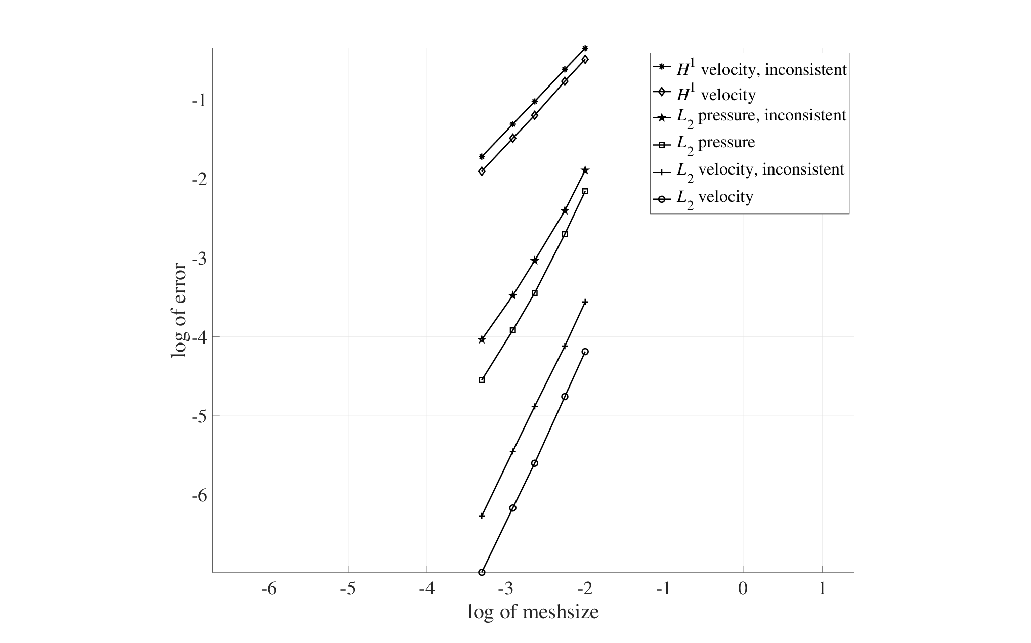
with ${\boldsymbol{f}}={\bf 0}$. The exact solution is used as Dirichlet data and zero mean pressure is imposed by a Lagrange multiplier. We compare the convergence of the pressure inconsistent method, using $\tilde{b}({\boldsymbol{u}},q)$, to the pressure consistent method, using $b({\boldsymbol{u}},q)$, in Fig. 3. The convergence is shown in $L_{2}$ for the pressure and the velocity and in broken $H^{1}$ semi–norm for the velocity. We note that the methods converge at the same rate, albeit with a slightly larger error constant for the inconsistent method. The observed rates from Fig. 3 are

As we do not have full $P^{2}$ approximation for the velocity, the observed rate of convergence of pressure is better than expected.

In Fig. 4 we compare the pressure solutions to the interpolated pressure on the boundary, shown on the finest mesh in the sequence used for the convergence study.

In this example we show that the strain formulation of Stokes equations poses no problem as we have a Korn inequality for our approximation. We consider a Poiseuille type problem in the domain $\Omega=(0,3)\times(0,1)\times(0,1/10)$ with boundary conditions ${\boldsymbol{u}}=(x_{2}(1-x_{2}),0,0)$ at $x_{1}=0$, at $x_{2}=0$, and at $x_{2}=1$, and with $u_{3}=0$ at $x_{3}=0$ and at $x_{3}=1/10$. In Fig. 6 we show the velocity field in the $(x_{1},x_{2})$–plane and we note that the strain formulation gives a stress free condition at the outflow. In Fig. 6 we show the corresponding pressure. The computations were made using the $\tilde{b}$–form of the side condition.

References

• [1] F. Brezzi and M. Fortin. Mixed and hybrid finite element methods, volume 15 of Springer Series in Computational Mathematics. Springer-Verlag, New York, 1991.
• [2] M. Crouzeix and P.-A. Raviart. Conforming and nonconforming finite element methods for solving the stationary Stokes equations. I. Revue Française Automatique Informatique Recherche Opérationnelle Série Rouge, 7(R-3):33–75, 1973.
• [3] P. Hansbo. A nonconforming rotated Q1Q_{1} approximation on tetrahedra. Computer Methods in Applied Mechanics and Engineering, 200(9-12):1311–1316, 2011.
• [4] P. Hansbo. Nonconforming rotated Q1Q_{1} tetrahedral element with explicit time stepping for elastodynamics. Internat. J. Numer. Methods Engrg., 91(10):1105–1114, 2012.
• [5] P. Hansbo and F. Larsson. The nonconforming linear strain tetrahedron for a large deformation elasticity problem. Comput. Mech., 58(6):929–935, 2016.
• [6] R. Rannacher and S. Turek. Simple nonconforming quadrilateral Stokes element. Numerical Methods for Partial Differential Equations, 8(2):97–111, 1992.
• [7] C. Taylor and P. Hood. A numerical solution of the Navier–Stokes equations using the finite element technique. Computers & Fluids, 1(1):73–100, 1973.
• [8] R. Verfürth. Error estimates for a mixed finite element approximation of the Stokes equations. RAIRO Anal. Numér., 18(2):175–182, 1984.