Proximal ADMM for Nonconvex and Nonsmooth Optimization

Yu Yang Email: yangyu21@xjtu.edu.cn Qing-Shan Jia Email: jiaqs@tsinghua.edu.cn Zhanbo Xu Email: zhanbo.xu@xjtu.edu.cn Xiaohong Guan Email: xhguan@xjtu.edu.cn Costas J. Spanos Email: spanos@berkeley.edu

Abstract

By enabling the nodes or agents to solve small-sized subproblems to achieve coordination, distributed algorithms are favored by many networked systems for efficient and scalable computation. While for convex problems, substantial distributed algorithms are available, the results for the more broad nonconvex counterparts are extremely lacking. This paper develops a distributed algorithm for a class of nonconvex and nonsmooth problems featured by i) a nonconvex objective formed by both separate and composite components regarding the decision variables of interconnected agents, ii) local bounded convex constraints, and iii) coupled linear constraints. This problem is directly originated from smart buildings and is also broad in other domains. To provide a distributed algorithm with convergence guarantee, we revise the powerful alternating direction method of multiplier (ADMM) method and proposed a proximal ADMM. Specifically, noting that the main difficulty to establish the convergence for the nonconvex and nonsmooth optimization with ADMM is to assume the boundness of dual updates, we propose to update the dual variables in a discounted manner. This leads to the establishment of a so-called sufficiently decreasing and lower bounded Lyapunov function, which is critical to establish the convergence. We prove that the method converges to some approximate stationary points. We besides showcase the efficacy and performance of the method by a numerical example and the concrete application to multi-zone heating, ventilation, and air-conditioning (HVAC) control in smart buildings.

keywords

distributed nonconvex and nonsmooth optimization, proximal ADMM, bounded Lagrangian multipliers, global convergence, smart buildings.

^†^†thanks: [^†^†address: School of Automation Science and Engineering, Xi’an Jiaotong University, Shaanxi, China.^†^†address: CFINS, Department of Automation, BNRist, Tsinghua University, Beijing, China.^†^†address: Electrical Engineering and Computer Sciences, University of California, Berkeley.

footnoteinfo] This work is supported by the Republic of Singapore’s National Research Foundation through a grant to the Berkeley Education Alliance for Research in Singapore (BEARS) for the Singapore-Berkeley Building Efficiency and Sustainability in the Tropics (SinBerBEST) Program. This work is also supported in part by National Natural Science Foundation of China (62192752, 62192750, 62125304, 62073182), 111 International Collaboration Project (BP2018006), and Tsinghua University Initiative Scientific Research Program.
Yu Yang is the corresponding author.

, , , ,

1 Introduction

By enabling the nodes or agents to solve small-sized subproblems to achieve coordination, distributed algorithms are favored by many networked systems to achieve efficient and scalable computation. While distributed algorithms for convex optimization have been studied extensively [1, 2, 3], the results for the more broad nonconvex counterparts are extremely lacking. The direct extension of distributed algorithms for convex problems to nonconvex counterparts is in general not applicable either due to the failure of convergence or the lack of theoretical convergence guarantee ( see [4, 5] for some divergent examples). This paper focuses on developing a distributed algorithm for a class of nonconvex and nonsmooth problems in the canonical form of


$\displaystyle\min_{\mathbf{x}=(\mathbf{x}_{i})_{i=1}^{N}}$	$\displaystyle F(\mathbf{x})=g(\mathbf{x})+\sum_{i=1}^{N}f_{i}(\mathbf{x}_{i})$	( $\mathbf{P}$ )
$\displaystyle{\rm s.t.}~$	$\displaystyle\sum_{i=1}^{N}\mathbf{A}_{i}\mathbf{x}_{i}=\mathbf{b}.$	(1a)
	$\displaystyle\mathbf{x}_{i}\in\mathbf{X}_{i},~i=1,2,\cdots,N.$	(1b)

where $i=1,2,\cdots,N$ denotes the computing nodes or agents, $\mathbf{x}_{i}\in\mathbf{R}^{n_{i}}$ is the local decision variables of agent $i$ and $\mathbf{x}=(\mathbf{x}_{i})_{i=1}^{N}\in\mathbf{R}^{n}$ with $n={\textstyle\sum}_{i=1}^{N}n_{i}$ stacks the decision variables of all agents. We have $f_{i}:\mathbf{R}^{n_{i}}\rightarrow\mathbf{R}$ and $g:\mathbf{R}^{n}\rightarrow\mathbf{R}$ denote the separate and composite objective components, which are continuously differentiable but possibly nonconvex. We have $\mathbf{X}_{i}$ represent the local bounded and convex constraints of agent $i$ . As expressed by the formulation, the agents are expected to optimize their local decision variables in a cooperative manner so as to achieve the optimal system performance measured by $F(\mathbf{x})=g(\mathbf{x})+{\textstyle\sum}_{i=1}^{N}f_{i}(\mathbf{x}_{i})$ considering both their local constraints $\mathbf{X}_{i}$ and the global coupled linear constraints (1a) encoded by $\mathbf{A}_{i}\in\mathbf{R}^{m\times n_{i}}$ and $b\in\mathbf{R}^{m}$ . By defining $\mathbf{A}=(\mathbf{A}_{1},\mathbf{A}_{2},\cdots,\mathbf{A}_{N})\in\mathbf{R}^{m\times n}$ and $f(\mathbf{x})=\sum_{i=1}^{N}f_{i}(\mathbf{x}_{i})$ , the coupled constraints and objective can be expressed by $\mathbf{A}\mathbf{x}=\mathbf{b}$ and $F(\mathbf{x})=f(\mathbf{x})+g(\mathbf{x})$ . Note that the presence of local constraints $\mathbf{X}_{i}$ and nonconvex objectives $f_{i}$ and $g$ makes the problem nonconvex and nonsmooth, which represents the major challenge to develop distributed algorithm with convergence guarantee.

Problem ( P ) is directly originated from smart buildings where smart devices are empowered to make local decisions while accounting for the interactions or the shared resource limits with the other devices in the proximity (see, for examples [6, 7]). Many other applications also fit into this formulation, including but not limited to smart sensing [8], energy storage sharing [9, 10], electric vehicle charging management [11, 12, 13, 14, 15, 16], peer-to-peer energy trading [17, 18], power system control [19], wireless communication control [20]. When the number of nodes is large, centralized methods usually suffer bottlenecks from the heavy computation, data storing and communication (see [6, 19, 20] and the references therein). Also, centralized methods may disrupt privacy as the complete information of all agents (e.g., the private local objectives) are required by a central computing agent. As a result, distributed algorithms are usually preferred for privacy, computing efficiency, small data storage, and scaling properties.

When problem ( P ) is convex, plentiful distributed solution methods are available. The methods can be distinguished by the presence of the composite objective component $g$ and the number of decision blocks $N$ . When $g$ is null, we have the classic dual decomposition methods [21, 22], the well-known alternating direction method of multiplier (ADMM) for two decision blocks ( $N=2$ ) [23] and the variations for multi-block settings ( $N\geq 3$ )[24, 25, 26]. While the classic ADMM and its variations propose to update the decision components in a sequential manner (usually called Gauss-Seidel decomposition), the works [2] and [27] have made some effort in developing parallel ADMM and its variations (usually called Jacobian ADMM or parallel ADMM). The above methods are generally limited to separable objective functions (i.e., only $f_{i}$ exist and $g=0$ ). For the general case with composite objective component $g$ , linearized ADMM [28] and inexact linearized ADMM [29] are also studied.

The above results are all for convex problems. Nevertheless, massive applications arising from the engineering systems and machine learning domains require to handle the type of problem ( P ) with possibly nonconvex objectives $f_{i}$ and $g$ . The non-convexity may originate from the complex system performance metrics or the penalties imposed on the operation constraints. When the objectives $f_{i}$ and $g$ lack convexity (i.e., the monotonically non-decreasing property of gradients or subgradients is lost), developing distributed methods with theoretical convergence guarantee becomes a much more challenging problem. Though some fresh distributed methods for constrained nonconvex problems have been developed, they can not be applied to problem ( P ) due to the nonsmoothness caused by the local constraints $\mathbf{X}_{i}$ . This can be perceived from the following literature.

Table 1: Distributed constrained nonconvex optimization

# Type	Problem structures	Main assumptions	Methods	Scheme	Convergence	Papers
1	$\begin{aligned} &\min_{(\mathbf{x}_{i})_{i=1}^{N}}\sum_{i=1}^{N}f_{i}(\mathbf{x}_{i})\\ &{\rm s.t.}~\sum_{i=1}^{N}\mathbf{A}_{i}\mathbf{x}_{i}=\mathbf{b}.\\ &\mathbf{x}_{i}\in\mathbf{X}_{i},~i=1,2,\cdots,N.\end{aligned}$	$f_{i}$ continuously differentiable. Strong second-order optimality condition.	ADAL	Jacobian	Local convergence. Local optima.	[27]
2	$\begin{aligned} &\min_{\mathbf{x}=(\mathbf{x}_{i})_{i=0}^{p},y}\!\!\!\!g(\mathbf{x})\!+\!\sum_{i=0}^{p}f_{i}(\mathbf{x}_{i})\!+\!h(\mathbf{y})\\ &{\rm s.t.}~\sum_{i=0}^{p}\mathbf{A}_{i}\mathbf{x}_{i}+\mathbf{B}\mathbf{y}=0.\\ \end{aligned}$	$g$ and $h$ Lipschitz continuous gradient. $f_{i}$ weakly convex. $\text{Im}(\mathbf{A})\subseteq\text{Im}(\mathbf{B})$ .	ADMM	Gauss-Seidel	Global convergence. Stationary points.	[5, 30] [31, 32]
3	$\begin{aligned} &\min_{\mathbf{x}=(\mathbf{x}_{i})_{i=1}^{N},y}\!\!\!\!\!\!g(\mathbf{x},\mathbf{y})\!\!+\!\!\sum_{i=1}^{N}\!f_{i}(\mathbf{x}_{i})\!+\!h(\mathbf{y})\\ &{\rm s.t.}~\sum_{i=1}^{N}\mathbf{A}_{i}\mathbf{x}_{i}+\mathbf{B}\mathbf{y}=0.\\ \end{aligned}$	$g$ and $h$ Lipschitz continuous gradient. $\text{Im}(\mathbf{A})\subseteq\text{Im}(\mathbf{B})$ .	Linearized ADMM	Gauss-Seidel	Global convergence. Stationary points.	[33]
4	$\begin{aligned} &\min_{(\mathbf{x}_{k})_{k=0}^{K}}\sum_{k=1}^{k}g_{k}(\mathbf{x}_{k})+h(\mathbf{x}_{0})\\ &{\rm s.t.}~\mathbf{x}_{k}=\mathbf{x}_{0}.\\ &\mathbf{x}_{0}\in\mathbf{X}.\end{aligned}$	$g$ Lipschitz continuous gradient. $h$ convex.	Flexible ADMM	Gauss-Seidel	Global convergence. Stationary points.	[34]
5	$\begin{aligned} &\min_{(\mathbf{x}_{k})_{k=0}^{K}}\sum_{k=1}^{N}g_{x}(\mathbf{x}_{k})+\ell(\mathbf{x}_{0})\\ &{\rm s.t.}~\sum_{k=1}^{K}\mathbf{A}_{k}\mathbf{x}_{k}=\mathbf{x}_{0}.\\ &\mathbf{x}_{k}\in\mathbf{X}_{k},~k=1,\cdots,N.\end{aligned}$	$\ell$ $\Lips$ continuous gradient. $g$ nonconvex but smooth or convex but non-smooth.	Flexible ADMM	Gauss-Seidel	Global convergence. Stationary points.	[34]
6	$\begin{aligned} &\min_{(\mathbf{x}_{i})_{i=1}^{N},\bar{\mathbf{x}}}\sum_{i=1}^{N}f_{i}(\mathbf{x}_{i})\\ &{\rm s.t.}~\sum_{i=1}^{N}\mathbf{A}_{i}\mathbf{x}_{i}+\mathbf{B}\bar{\mathbf{x}}=0.\\ &\mathbf{x}_{i}\in\mathbf{X}_{i},h_{i}(\mathbf{x}_{i})=0,\\ &\quad\quad i=1,\cdots,N.\\ &\bar{\mathbf{x}}\in\bar{\mathbf{X}}.\end{aligned}$	$f_{i}$ continuously differentiable. $h_{i}$ non-linear (possibly nonconvex). $\mathbf{B}$ full column rank. $\mathbf{X}_{i}$ possibly nonconvex.	ALM + ADMM	Gauss-Seidel	Global convergence. Stationary points.	[35, 36, 37]
7	$\begin{aligned} &\min_{(\mathbf{x}_{i})_{i=1}^{N}}g(\mathbf{x})+\sum_{i=1}^{N}f_{i}(\mathbf{x}_{i})\\ &{\rm s.t.}~\sum_{i=1}^{N}\mathbf{A}_{i}\mathbf{x}_{i}=\mathbf{b}.\\ &\mathbf{x}_{i}\in\mathbf{X}_{i},~i=1,2,\cdots,N.\end{aligned}$	$f_{i}$ and $g$ Lipschitz continuous gradient.	Proximal ADMM	Jacobian	Global convergence. Approximate stationary points.	This paper

Note: the set

\mathbf{X}_{i}

and

\bar{\mathbf{X}}

are bounded convex sets.

A comprehensive survey of ADMM for constrainted optimization is available [38]. The existing works for constrained nonconvex optimization can be distinguished by problem structures, main assumptions, decomposition scheme (i.e., Jacobian or Gaussian-Seidel) and convergence guarantee as reported in Table 1. Overall, they can be uniformly expressed by the template of problem ( P ) but are slightly different in the settings and assumptions.

The first category (Type 1) is concerned with problem ( P ) without any composite objective component $g$ [27]. An accelerated distributed augmented Lagrangian (ADAL) method was proposed to handle the possibly nonconvex but continuously differentiable objectives $f_{i}$ . This method follows the classic ADMM framework but introduces an interpolation procedure regarding the primal updates at each iteration, which reads as $\mathbf{A}_{i}\mathbf{x}_{i}^{k+1}=\mathbf{A}_{i}\mathbf{x}_{i}^{k}+\mathbf{T}\left(\mathbf{A}_{i}\hat{\mathbf{x}}^{k}_{i}-\mathbf{A}_{i}\mathbf{x}^{k}_{i}\right)$ ( $k$ the iteration and $\mathbf{T}$ is a weighted matrix). To our understanding, this can be interpreted as a means to slow down the primal update for enhancing the convergence in nonconvex settings. By assuming the existence of stationary points that satisfy the strong second-order optimality condition, this paper established the local convergence of the method. The notion of local convergence is that the convergence towards some local optima can be assured if starting with a point sufficiently close to that local optima.

The subsequent four categories (Type 2, 3, 4, 5) differ from the first one mainly in the presence of a last block encoded by $\mathbf{B}$ . Note that [34] can be viewed as a special case with $\mathbf{B}=\mathbf{I}$ , where $\mathbf{I}$ are identity matrices of suitable sizes. The last block is exceptional due to the unconstrained and $\Lips$ differentiable property, which are critical to bound the dual updates for establishing convergence (see the references therein). That’s why the last decision block is usually distinguished by some special notations (i.e., $\mathbf{y}$ , $\mathbf{x}_{0}$ ). While the first category employs Jacobian decomposition for primal update, these four categories fall into Gauss-Seidel decomposition (i.e., alternating minimization). Specially, the works [5] and [33] have made some effort in handling possible composite objective components $g$ but via different ways. Specifically, [5] employed block coordinate and [33] used linearization technique. Particularly, [34, 5] build a general framework to establish the convergence for Gauss-Seidel ADMM towards local optima or stationary points in nonconvex settings, which comprises two key steps: 1) identifying a so-called sufficiently decreasing Lyapunov function, and 2) establishing the lower boundness property of the Lyapunov function. The sufficiently decreasing and lower boundness property of a proper Lyapunov function state that [5]

\begin{split}&T(\mathbf{x}^{k+1},\bm{\lambda}^{k+1})-T(\mathbf{x}^{k},\bm{\lambda}^{k})\\ &\quad\quad\quad\leq-a_{\mathbf{x}}\|\mathbf{x}^{k+1}-\mathbf{x}^{k}\|^{2}-a_{\bm{\lambda}}\|\bm{\lambda}^{k+1}-\bm{\lambda}^{k}\|^{2}.\\ &T(\mathbf{x}^{k},\bm{\lambda}^{k})>-\infty.\end{split}

(2)

where $T(\cdot,\cdot)$ is a general Lyapunov function, $\mathbf{x}$ and $\bm{\lambda}$ are primal and dual variables, $a_{\mathbf{x}}$ and $a_{\bm{\lambda}}$ are positive coefficients. The augmented Lagrangian (AL) function has been often used as the Lyapunov function in nonconvex settings (see [34, 5] and the references therein). However, they depend on the following two necessary conditions on the last decision block encoded by $\mathbf{B}$ to bound the dual updates $\|\bm{\lambda}^{k+1}-\bm{\lambda}^{k}\|^{2}$ by the primal updates $\|\mathbf{x}^{k+1}-\mathbf{x}^{k}\|^{2}$ [34, 5].

a)

$\mathbf{B}$ has full column rank and $\text{Im}(\mathbf{A})\subseteq\text{Im}(\mathbf{B})$ ( $\text{Im}(\cdot)$ represents the image of a matrix).
b)

The last decision block is unconstrained and with $\Lips$ differentiable objective.

Noted that the forth and fifth category (Type 4, 5) originated from [34] are a special case with $\mathbf{B}=\mathbf{I}$ and thus satisfy the necessary condition a).

Following the line of works, the sixth category (Type 6) studied the extension of ADMM to non-linearly constrained nonconvex problems [35, 36, 37]. Since it is difficult (if not impossible) to directly handle the non-linear couplings by the AL framework, [35] proposed to first convert the non-linearly constrained problems to linearly constrained ones by introducing decision copies for interconnected agents. This yields linearly constrained nonconvex problems with local non-linear constraints. The work [35] argues that the direct extension of ADMM to the reformulated problem is not applicable for the two necessary conditions condition a) and b) can not be satisfied simultaneously. To bypass the challenge, [35] proposed to introduce a block of slack variables working as the last block. To force the slack block to zero, this paper developed a two-level method where the inner-level uses classic ADMM to solve a relaxed problem with a penalty on the slack variables , and the outer-level gradually forces the slack variables towards zero.

As can be perceived from the literature, it is difficult (if not impossible) to develop a distributed method with convergence guarantee for ( P ) due to the lack of a well-behaved last block satisfying condition a) and b). The work [27] provided a solution with local convergence guarantee but can not handle the probable composite objective components $g$ . Though the idea of introducing slack variables in [35] can provide a solution with global convergence guarantee but at the cost of heavy iteration complexity caused by the two-level structure. Despite these limitations, what we can learn from the literature is that the behaviors of dual variables is important to draw the convergence of ADMM for nonconvex problems.

This paper focuses on developing a distributed method for problem ( P ) with theoretical convergence guarantee. Our main contributions are

•

We propose a proximal ADMM by revising the dual update procedure of classic ADMM into a discounted manner. This leads to the boundness of dual updates, which is critical to establish the convergence.
•

We establish the global convergence of the method towards approximate stationary points by identifying a proper Lyapunov function which is sufficiently decreasing and lower bounded as required.
•

We showcase the performance of the distributed method with a numerical example and a concrete application arising from smart buildings, which demonstrate the method’s effectiveness.

The reminder of this paper is organized as follows. In Section 2, we present the proximal ADMM. In Section 3, we study the convergence of the method. In Section 4, we showcase the method’s performance with a numerical example and smart building application. In Section 5, we conclude this paper and discuss the future work.

2 Proximal ADMM

2.1 Notations

Throughout the paper, we will visit the following notations. We use the bold alphabets $\mathbf{x},\mathbf{y},\mathbf{a},\mathbf{b},\mathbf{c}$ and $\mathbf{A},\mathbf{A}_{i},\mathbf{Q},\mathbf{M}$ to represent vectors and matrices. We define $\mathbf{I}_{n}$ or $\mathbf{I}$ as identity matrices of $n\times n$ or suitable size. We use the operator $:=$ to give definitions. We have $\mathbf{R}^{n}$ represent the $n$ -dimensional real space and $(\mathbf{x}_{i})_{i=1}^{N}:=(\mathbf{x}_{1}^{\top},\mathbf{x}_{2}^{\top},\cdots,\mathbf{x}_{N}^{\top})^{\top}$ is the stack of sub-vector $\mathbf{x}_{i}\in\mathbf{R}^{n_{i}}$ . We refer to $\|\!\cdot\!\|$ as Euclidean norm without specification, i.e., $\|\mathbf{x}\|=\sqrt{{\textstyle\sum}_{i=1}^{n}x_{i}^{2}}$ for $\mathbf{x}\in\mathbf{R}^{n}$ , and $\langle\mathbf{x},\mathbf{y}\rangle$ denote the dot product of vector $\mathbf{x},\mathbf{y}\in\mathbf{R}^{n}$ . We besides have $\|\mathbf{x}\|^{2}_{\mathbf{A}}=\mathbf{x}^{\top}\mathbf{A}\mathbf{x}$ . We use $\text{diag}(\mathbf{A}_{1},\mathbf{A}_{2},\cdots,\mathbf{A}_{N})$ to denote the diagonal matrix formed by the sub-matrices $\mathbf{A}_{1},\mathbf{A}_{2},\cdots,\mathbf{A}_{N}$ . We have the normal cone to a convex set $\mathbf{X}\subseteq\mathbf{R}^{n}$ at $\mathbf{x}^{*}$ defined by $N_{\mathbf{X}}(\mathbf{x}^{*}):=\{\nu\in\mathbf{R}^{n}|\langle\nu,\mathbf{x}-\mathbf{x}^{*}\rangle\leq 0,\forall\mathbf{x}\in\mathbf{X}\}$ . For $g:\mathbf{R}^{n}\rightarrow\mathbf{R}$ and $\mathbf{x}=(\mathbf{x}_{i})_{i=1}^{N}\in\mathbf{R}^{n}$ , we denote $\nabla_{i}g(\mathbf{x})=\nabla_{\mathbf{x}_{i}}g(\mathbf{x})$ as the partial differential of $g$ with respect to component $\mathbf{x}_{i}\in\mathbf{R}^{n_{i}}$ . We define ${\rm dist}(\mathbf{x},\mathbf{X})=\min_{\mathbf{y}\in\mathbf{X}}\|\mathbf{x}-\mathbf{y}\|$ as the distance of vector $\mathbf{x}\in\mathbf{R}^{n}$ to the subset $\mathbf{X}\subseteq\mathbf{R}^{n}$ .

2.2 Algorithm

In this part, we introduce the proximal ADMM for solving problem ( P ) in a distributed manner. The proximal ADMM is a type of AL methods that depend on the AL technique to relax constraints and employ the primal-dual scheme to update variables. By defining Lagrangian multipliers $\bm{\lambda}\in\mathbf{R}^{m}$ for the coupled constraints (1a), we have the AL function for problem ( P )

\displaystyle\mathbb{L}_{\rho}(\mathbf{x},\bm{\lambda})=

\displaystyle F(\mathbf{x})+\left\langle\bm{\lambda},\mathbf{A}\mathbf{x}-\mathbf{b}\right\rangle\!+\!\frac{\rho}{2}\|\mathbf{A}\mathbf{x}-\mathbf{b}\|^{2}

(3)

where $F(\mathbf{x})=g(\mathbf{x})+\sum_{i=1}^{N}f_{i}(\mathbf{x}_{i})$ and $\rho$ is the penalty parameter.

Following the standard AL methods, the proximal ADMM is composed of Primal update and Dual update as shown in Algorithm 1. In Primal update, the primal variables $\mathbf{x}=(\mathbf{x}_{i})_{i=1}^{N}$ are updated in a distributed manner via Jacobian decomposition. Particularly, to handle the composite objective component $g$ , we linearize the composite term at each iteration $k$ by $g(\mathbf{x}^{k})+\langle\nabla g(\mathbf{x}^{k}),\mathbf{x}-\mathbf{x}^{k}\rangle$ (the constant part $g(\mathbf{x}^{k})$ is dropped). Note that the local objective terms $f_{i}$ can also be linearized similarly if necessary and the proof of this paper still applies. To favor computation efficiency and scaling properties, we adopt the Jacobian scheme and empower the agents to update their decision components in parallel at each iteration with the preceding information from their interconnected agents. Particularly, to enhance convergence, a proximal term $\|\mathbf{x}_{i}-\mathbf{x}_{i}^{k+1}\|^{2}$ is imposed on the local objective of each agent (Step 3). This has been used in many Jacobian ADMM both in convex [39, 2, 40] and nonconvex [33, 41] settings. Note that the subproblems (6) are either convex or nonconvex optimization over the local constraints $\mathbf{X}_{i}$ , depending on $f_{i}$ . There are many first-order solvers to solve those subproblems, such as the projected gradient method [42] and the proximal gradient method [43]. This paper focuses on developing a general distribute framework for solving problem ( P ) and will not discuss the subproblems in detail. The major difference of the proximal ADMM from the existing distributed AL methods is that we have modified the Dual update by imposing a discounting factor $(1-\tau)$ ( $\tau\in[0,1)$ ) (Step 4). The idea and motivation behind are to update the dual variables by the constraints residual in a discounted manner so as to bound the dual variables in the iterative process, which has been identified as critical to draw theoretical convergence. In this setting, the dual variables are the discounted running sum of the constraints residual, i.e.,

\begin{split}\bm{\lambda}^{k+1}&=(1-\tau)\bm{\lambda}^{k}+\rho(\mathbf{A}\mathbf{x}^{k+1}-\mathbf{b})\\ &=(1-\tau)^{2}\bm{\lambda}^{k-1}+(1-\tau)\rho(\mathbf{A}\mathbf{x}^{k}-\mathbf{b})\\ &\hskip 9.24994pt\hskip 9.24994pt\hskip 9.24994pt\hskip 9.24994pt\hskip 9.24994pt\hskip 9.24994pt\hskip 9.24994pt+\rho(\mathbf{A}\mathbf{x}^{k+1}-\mathbf{b})\\ &\cdots\\ &=(1-\tau)^{k+1}\bm{\lambda}^{0}+{\textstyle\sum}_{\ell=0}^{k}(1-\tau)^{k-\ell}\rho(\mathbf{A}\mathbf{x}^{\ell+1}-\mathbf{b}).\end{split}

(4)

This differs from classic ADMM where the dual variables are the running sum of the constraints residual, i.e.,

	$\displaystyle\bm{\lambda}^{k+1}$	$\displaystyle=\bm{\lambda}^{k}+\rho(\mathbf{A}\mathbf{x}^{k+1}-\mathbf{b})$
		$\displaystyle=\bm{\lambda}^{k-1}+\rho(\mathbf{A}\mathbf{x}^{k}-\mathbf{b})+\rho(\mathbf{A}\mathbf{x}^{k+1}-\mathbf{b})$
		$\displaystyle\cdots$
		$\displaystyle=\bm{\lambda}^{0}+{\textstyle\sum}_{\ell=0}^{k}\rho(\mathbf{A}\mathbf{x}^{\ell+1}-\mathbf{b}).$

From this perspective, classic ADMM can be viewed as a special case of the proximal ADMM with $\tau=0$ . In the proximal ADMM, the Primal update and Dual update are alternated until the stopping criterion

\displaystyle\|T_{c}^{k+1}-T_{c}^{k}\|\leq\epsilon

(5)

is reached, where $T_{c}^{k}$ is the Lyapunov function to be discussed later. The parameter $\epsilon$ is a user-defined positive threshold.

Algorithm 1 Proximal ADMM for problem ( P )

1: Initialize:

\mathbf{x}^{0}

\mathbf{\bm{\lambda}}^{0}

and

\rho>0

\tau\in[0,1)

, and set

k\rightarrow 0

2: Repeat:

3: Primal update:

\begin{split}&\mathbf{x}_{i}^{k+1}\!=\!\arg\!\min_{\mathbf{x}_{i}\in\mathbf{X}_{i}}\!\!\left\{\begin{array}[]{l}\langle\nabla_{i}g(\mathbf{x}^{k}),\mathbf{x}_{i}-\mathbf{x}_{i}^{k}\rangle\\ \!+f_{i}(\mathbf{x}_{i})+\langle\bm{\lambda}^{k},\mathbf{A}_{i}\mathbf{x}_{i}^{k}\rangle\\ \!+\rho/2\|\mathbf{A}_{i}\mathbf{x}_{i}\!+\!\!{\textstyle\sum}_{j\neq i}\mathbf{A}_{j}\mathbf{x}_{j}^{k}\!-\!\mathbf{b}\|^{2}\\ \!+\beta/2\|\mathbf{x}_{i}-\mathbf{x}_{i}^{k}\|^{2}_{\mathbf{B}_{i}}\end{array}\right\}\\ \end{split}

(6)

4: Dual update:

\displaystyle\bm{\lambda}^{k+1}

\displaystyle\!=\!(1-\tau)\bm{\lambda}^{k}\!+\!\rho\left(\mathbf{A}\mathbf{x}^{k+1}\!-\!\mathbf{b}\right)

(7)

5: Until the stopping criterion (5) is reached.

3 Convergence Analysis

Before establishing the convergence of Algorithm 1, we first clarify the main assumptions.

3.1 Main assumptions

(A1)

Function $f\!:\!\mathbf{R}^{n}\rightarrow\mathbf{R}$ and $g:\mathbf{R}^{n}\rightarrow\mathbf{R}$ have $\Lips$ continuous gradient (i.e., $\Lips$ differentiable) with modulus $L_{f}$ and $L_{g}$ over the set $\mathbf{X}=\mathbf{X}_{1}\times\mathbf{X}_{2}\times\cdots\times\mathbf{X}_{N}$ , i.e., [31]

		$\displaystyle\\|\nabla f(\mathbf{x})-\nabla f(\mathbf{y})\\|\leq L_{f}\\|\mathbf{x}-\mathbf{y}\\|,~\forall\mathbf{x},\mathbf{y}\in\mathbf{X}.$
		$\displaystyle\\|\nabla g(\mathbf{x})-\nabla g(\mathbf{y})\\|\leq L_{g}\\|\mathbf{x}-\mathbf{y}\\|,~\forall\mathbf{x},\mathbf{y}\in\mathbf{X}.$

(A2)

Function $\!f\!:\mathbf{R}^{n}\!\!\rightarrow\!\mathbf{R}$ and $g\!:\mathbf{R}^{n}\!\rightarrow\!\!\mathbf{R}$ are lower bounded over the set $\mathbf{X}\!=\!\mathbf{X}_{1}\!\times\!\mathbf{X}_{2}\times\!\cdots\!\times\!\mathbf{X}_{N}$ , i.e.,

	$\displaystyle f(\mathbf{x})$	$\displaystyle>-\infty,~~\forall\mathbf{x}\in\mathbf{X}.$
	$\displaystyle g(\mathbf{x})$	$\displaystyle>-\infty,~~\forall\mathbf{x}\in\mathbf{X}.$

3.2 Main results

As discussed, there are two key steps to draw convergence for a distributed AL method in nonconvex settings: 1) identifying a so-called sufficiently decreasing Lyapunov function; and 2) establishing the lower boundness property of the Lyapunov function. To achieve the objective, we first draw the following two propositions.

Proposition 1

For the sequences $\{\mathbf{x}^{k}\}_{k\in\mathbf{K}}$ and $\{\bm{\lambda}^{k}\}_{k\in\mathbf{K}}$ generated by Algorithm 1, we have

\begin{split}&\frac{1-2\tau^{2}}{2\rho}\left\|\bm{\lambda}^{k+1}-\bm{\lambda}^{k}\right\|^{2}+\frac{1}{2}\|\mathbf{x}^{k+1}-\mathbf{x}^{k}\|^{2}_{\mathbf{Q}}\\ &\quad+\frac{L_{g}}{2}\|\mathbf{x}^{k+1}-\mathbf{x}^{k}\|^{2}+\frac{1}{2}\|\mathbf{w}^{k}\|^{2}_{\mathbf{Q}}\\ &\leq\frac{1-2\tau^{2}}{2\rho}\left\|\bm{\lambda}^{k}-\bm{\lambda}^{k-1}\right\|^{2}+\frac{1}{2}\|\mathbf{x}^{k}-\mathbf{x}^{k-1}\|^{2}_{\mathbf{Q}}\\ &\quad+\frac{L_{g}}{2}\|\mathbf{x}^{k}-\mathbf{x}^{k-1}\|^{2}+\rho_{F}\left\|\mathbf{x}^{k+1}-\mathbf{x}^{k}\right\|^{2}\\ &\quad-{\tau(1+\tau)}/{\rho}\|\bm{\lambda}^{k+1}-\bm{\lambda}^{k}\|^{2}.\end{split}

where we have the iterations $\mathbf{K}:=\{1,2,\cdots,K\}$ and

	$\displaystyle\mathbf{w}^{k}:$	$\displaystyle=(\mathbf{x}^{k+1}-\mathbf{x}^{k})-(\mathbf{x}^{k}-\mathbf{x}^{k-1})$
	$\displaystyle G_{\mathbf{A}}:$	$\displaystyle=\text{diag}\left(\mathbf{A}_{1}^{\top}\mathbf{A}_{1},\cdots,\mathbf{A}_{N}^{\top}\mathbf{A}_{N}\right)$
	$\displaystyle G_{\mathbf{B}}:$	$\displaystyle=\text{diag}\left(\mathbf{B}_{1}^{\top}\mathbf{B}_{1},\cdots,\mathbf{B}_{N}^{\top}\mathbf{B}_{N}\right)$
	$\displaystyle\mathbf{Q}:$	$\displaystyle=\rho G_{\mathbf{A}}+\beta G_{\mathbf{B}}-\rho\mathbf{A}^{\top}\mathbf{A}$
	$\displaystyle\rho_{F}:$	$\displaystyle=L_{f}+L_{g}.$

Proof of Prop. 1: We defer the proof to Appendix A.

Let $\mathbb{L}^{+}_{\rho}(\mathbf{x},\bm{\lambda}):=\mathbb{L}_{\rho}(\mathbf{x},\bm{\lambda})-\frac{\tau}{2\rho}\|\bm{\lambda}\|^{2}$ be the regularized AL function. We have the subsequent proposition to quantify the change of regularized AL function over the successive iterations.

Proposition 2

For the sequences $\{\mathbf{x}^{k}\}_{k\in\mathbf{K}}$ and $\{\bm{\lambda}^{k}\}_{k\in\mathbf{K}}$ generated by Algorithm 1, we have

\begin{split}&\mathbb{L}^{+}_{\rho}(\mathbf{x}^{k+1},\bm{\lambda}^{k+1})-\mathbb{L}^{+}_{\rho}(\mathbf{x}^{k},\bm{\lambda}^{k})\\ &\leq-\|\mathbf{x}^{k+1}-\mathbf{x}^{k}\|_{\mathbf{Q}}^{2}+\frac{\rho_{F}}{2}\|\mathbf{x}^{k+1}-\mathbf{x}^{k}\|^{2}\!\\ &\quad-\frac{\rho}{2}\|\mathbf{A}(\mathbf{x}^{k+1}-\mathbf{x}^{k})\|^{2}+\frac{2-\tau}{2\rho}\|\bm{\lambda}^{k+1}-\bm{\lambda}^{k}\|^{2}.\end{split}

Proof of Prop. 2: We defer the proof to Appendix B.

In the literature, the AL function is often used as the Lyapunov function if the sufficiently decreasing property can be established (see [5, 30, 31, 32] for examples). However, this is not the case for Algorithm 1. From Prop. 2, we note that the sufficiently decreasing property of the (regularized) AL function can be established if and only if the dual updates $\|\bm{\lambda}^{k+1}-\bm{\lambda}^{k}\|^{2}$ can be bounded by the primal updates $\|\mathbf{x}^{k+1}-\mathbf{x}^{k}\|^{2}$ (see the definition (2)). This is difficult (if not impossible) due to the lack of a well-behaved last block (i.e., unconstrained and $\Lips$ differentiable) as discussed.

However, by combing Prop. 1 and Prop. 2, we indeed can identify a sufficiently decreasing Lyapunov function. Specifically, from Prop. 2, we have the (regularized) AL function $\mathbb{L}^{+}_{\rho}(\mathbf{x}^{k+1},\bm{\lambda}^{k+1})$ is ascending in $\|\bm{\lambda}^{k+1}-\bm{\lambda}^{k}\|^{2}$ and descending in $\|\mathbf{x}^{k+1}-\mathbf{x}^{k}\|^{2}$ . This is exactly opposite to the descending and ascending properties of the term $\frac{1-2\tau^{2}}{2\rho}\|\bm{\lambda}^{k+1}-\bm{\lambda}^{k}\|^{2}+\frac{1}{2}\|\mathbf{x}^{k+1}-\mathbf{x}^{k}\|^{2}_{\mathbf{Q}}$ stated in Prop. 1. Note that this is attributed to the imposed discounted factor $\tau>0$ , otherwise the term $\tau(1-\tau)/\rho\|\bm{\lambda}^{k+1}-\bm{\lambda}^{k}\|^{2}$ in Prop. 1 would be zero. We therefore build the Lyapunov function as

		$\displaystyle T_{c}(\mathbf{x}^{k+1},\bm{\lambda}^{k+1};\mathbf{x}^{k},\bm{\lambda}^{k})=\mathbb{L}^{+}_{\rho}(\mathbf{x}^{k+1},\bm{\lambda}^{k+1})$
		$\displaystyle\quad~+c\bigg(\frac{1-2\tau^{2}}{2\rho}\\|\bm{\lambda}^{k+1}-\bm{\lambda}^{k}\\|^{2}+\frac{1}{2}\\|\mathbf{x}^{k+1}-\mathbf{x}^{k}\\|^{2}_{\mathbf{Q}}$
		$\displaystyle\quad~+\frac{L_{g}}{2}\\|\mathbf{x}^{k}-\mathbf{x}^{k-1}\\|^{2}\bigg)$		(8)

where $c$ is a constant parameter to be determined for ensuring the sufficiently decreasing and lower boundness property of the Lyapunov function.

Let $T_{c}^{k+1}:=T_{c}(\mathbf{x}^{k+1},\bm{\lambda}^{k+1};\mathbf{x}^{k},\bm{\lambda}^{k})$ be the Lyapunov function at iteration $k$ , we have the following proposition regarding the sufficiently decreasing property.

Proposition 3

For the sequences $\{\mathbf{x}^{k}\}_{k\in\mathbf{K}}$ and $\{\bm{\lambda}^{k}\}_{k\in\mathbf{K}}$ generated by Algorithm 1, we have

\begin{split}&T_{c}^{k+1}\!-\!T_{c}^{k}\leq-a_{\mathbf{x}}\|\mathbf{x}^{k+1}\!-\!\mathbf{x}^{k}\|^{2}\!-\!a_{\bm{\lambda}}\|\bm{\lambda}^{k+1}\!-\!\bm{\lambda}^{k}\|^{2}\!-\!\frac{c}{2}\|\mathbf{w}^{k}\|^{2}\end{split}

where we have $\rho_{F}=L_{f}+L_{g}$ and

\begin{split}&a_{\mathbf{x}}:=\frac{2\rho G_{\mathbf{A}}+2\beta G_{\mathbf{B}}-\rho\mathbf{A}^{\top}\mathbf{A}-(2c+1)\rho_{F}\mathbf{I}_{N}}{2}\\ &a_{\bm{\lambda}}:=\frac{2c\tau(1+\tau)-(2-\tau)}{2\rho}.\end{split}

Proof of Prop. 3: Based on Prop. 1 and Prop. 2, we have

		$\displaystyle T_{c}^{k+1}-T_{c}^{k}=-\\|\mathbf{x}^{k+1}-\mathbf{x}^{k}\\|_{\mathbf{Q}}^{2}+\frac{\rho_{F}}{2}\\|\mathbf{x}^{k+1}-\mathbf{x}^{k}\\|^{2}$
		$\displaystyle\quad-\frac{\rho}{2}\\|\mathbf{A}(\mathbf{x}^{k+1}-\mathbf{x}^{k})\\|^{2}+\frac{2-\tau}{2\rho}\\|\bm{\lambda}^{k+1}-\bm{\lambda}^{k}\\|^{2}$
		$\displaystyle\quad+c\Big(\rho_{F}\left\\|\mathbf{x}^{k+1}-\mathbf{x}^{k}\right\\|^{2}-{\tau(1+\tau)}/{\rho}\\|\bm{\lambda}^{k+1}-\bm{\lambda}^{k}\\|^{2}$
		$\displaystyle\quad-{1}/{2}\\|\mathbf{w}^{k}\\|^{2}_{\mathbf{Q}}\Big)$
		$\displaystyle\leq-a_{\mathbf{x}}\\|\mathbf{x}^{k+1}-\mathbf{x}^{k}\\|^{2}-a_{\bm{\lambda}}\\|\bm{\lambda}^{k+1}-\bm{\lambda}^{k}\\|^{2}-\frac{c}{2}\\|\mathbf{w}^{k}\\|^{2}_{\mathbf{Q}}$

where the inequality is directly derived by rearranging the terms. We therefore close the proof.

Remark 1

Prop. 3 implies that we would have the sufficiently decreasing property hold by the constructed Lyapunov function $T_{c}^{k}$ if we have $a_{\mathbf{x}}>0$ , $a_{\bm{\lambda}}>0$ , $c\geq 0$ and $\mathbf{Q}\geq 0$ . Actually, this can be achieved by setting the tuple ( $\tau$ , $\rho$ , $\beta$ , $\mathbf{B}_{i}$ , $c$ ) properly for Algorithm 1, which will be discussed shortly.

As discussed, another key step to draw the convergence is to establish the lower boundness property of the Lyapunov function. To this end, we first prove the lower boundness property of Lagrangian multipliers resulting from the discounted dual update scheme.

Proposition 4

Let $\Delta^{k}:=\|\mathbf{A}\mathbf{x}^{k}-\mathbf{b}\|$ be the constraints residual at iteration $k$ , $\Delta^{\max}:=\max_{\mathbf{x}\in\mathbf{X}}\|\mathbf{A}\mathbf{x}-\mathbf{b}\|$ denote the maximal constraints residual over the closed feasible set $\mathbf{X}$ , and Algorithm 1 start with any given initial dual variable $\bm{\lambda}^{0}$ , we have $\|\bm{\lambda}^{k}\|$ is bounded, i.e.,

\begin{split}&\|\bm{\lambda}^{k}\|\leq\|\bm{\lambda}^{0}\|+\tau^{-1}\rho\Delta^{\max}\\ \text{or}~~&\|\bm{\lambda}^{k}\|^{2}\leq 2\|\bm{\lambda}^{0}\|^{2}+2\tau^{-2}\rho^{2}(\Delta^{\max})^{2}.\end{split}

(9)

Proof of Prop. 4: Recall the dual update scheme in (4), we have

	$\displaystyle\\|\bm{\lambda}^{k}\\|$	$\displaystyle=\\|(1-\tau)^{k+1}\bm{\lambda}^{0}+{\textstyle\sum}_{\ell=0}^{k}\rho(1-\tau)^{k-\ell}\Delta^{\ell+1}\\|$
		$\displaystyle\leq\\|(1-\tau)^{k+1}\bm{\lambda}^{0}\\|+{\textstyle\sum}_{\ell=0}^{k}\\|\rho(1-\tau)^{k-\ell}\Delta^{\ell+1}\\|$
		$\displaystyle\leq\\|(1-\tau)^{k+1}\bm{\lambda}^{0}\\|+\rho\Delta^{\max}\frac{1-(1-\tau)^{k}}{\tau}$
		$\displaystyle\leq\\|\bm{\lambda}^{0}\\|+\tau^{-1}\rho\Delta^{\max}$

where the first inequality is by the triangle inequality of norm, the second inequality infers from $\Delta^{k}\leq\Delta^{\max},\forall k$ , and the last inequality holds because of $\tau\in(0,1)$ .

Further based on $\|\mathbf{a}+\mathbf{b}\|^{2}\leq 2\|\mathbf{a}\|^{2}+2\|\mathbf{b}\|^{2}$ , we directly have $\|\bm{\lambda}^{k}\|^{2}\leq 2\|\bm{\lambda}^{0}\|^{2}+2\tau^{-2}\rho^{2}(\Delta^{\max})^{2}$ . We therefore complete the proof.

Based on Prop. 4, we are able to establish the lower boundness property of Lyapunov function as below.

Proposition 5

For the sequences $\{\mathbf{x}^{k}\}_{k\in\mathbf{K}}$ and $\{\bm{\lambda}^{k}\}_{k\in\mathbf{K}}$ generated by Algorithm 1, we have

\displaystyle T_{c}^{k+1}>-\infty,\forall k\in\mathbf{K}.

(10)

Proof of Prop. 5: By examining the terms of $T_{c}^{k+1}$ in (3.2), we only require to establish the lower boundness property of $\mathbb{L}_{\rho}^{+}(\mathbf{x}^{k+1},\bm{\lambda}^{k+1})=\mathbb{L}_{\rho}(\mathbf{x}^{k+1},\bm{\lambda}^{k+1})-\frac{\tau}{2\rho}\|\bm{\lambda}^{k+1}\|^{2}$ for the other terms are all non-negative. Based on Prop. 4, we directly have $-\frac{\tau}{2\rho}\|\bm{\lambda}^{k+1}\|^{2}$ lower bounded since $\|\bm{\lambda}^{k+1}\|^{2}$ is upper bounded. We therefore only need to prove that $\mathbb{L}_{\rho}(\mathbf{x}^{k+1},\bm{\lambda}^{k+1})=f(\mathbf{x}^{k+1})+\langle\bm{\lambda}^{k+1},\mathbf{A}\mathbf{x}^{k+1}-b\rangle+{\rho}/{2}\left\|\mathbf{A}\mathbf{x}^{k+1}-\mathbf{b}\right\|^{2}$ is lower bounded. Note that we have $f(\mathbf{x}^{k+1})>-\infty$ over the compact set $\mathbf{X}$ (see (A2)) and the quadratic term non-negative. This infers we only need to prove the lower boundness for the second term $\langle\bm{\lambda}^{k+1},\mathbf{A}\mathbf{x}^{k+1}-b\rangle$ . Based on the dual update (7), we have

		$\displaystyle\langle\bm{\lambda}^{k+1},\mathbf{A}\mathbf{x}^{k+1}-\mathbf{b}\rangle=\left\langle\bm{\lambda}^{k+1},\frac{\bm{\lambda}^{k+1}-(1-\tau)\bm{\lambda}^{k}}{\rho}\right\rangle$
		$\displaystyle=\left\langle\bm{\lambda}^{k+1},\frac{1-\tau}{\rho}(\bm{\lambda}^{k+1}-\bm{\lambda}^{k})+\frac{\tau}{\rho}\bm{\lambda}^{k+1}\right\rangle$		(11)
		$\displaystyle=\frac{\tau}{\rho}\\|\bm{\lambda}^{k+1}\\|^{2}+\frac{1-\tau}{\rho}\left\langle\bm{\lambda}^{k+1},\bm{\lambda}^{k+1}-\bm{\lambda}^{k}\right\rangle$
		$\displaystyle=\frac{\tau}{\rho}\\|\bm{\lambda}^{k+1}\\|^{2}\!+\!\frac{1-\tau}{2\rho}\big(\\|\bm{\lambda}^{k+1}\!-\!\bm{\lambda}^{k}\\|^{2}\!+\!\\|\bm{\lambda}^{k+1}\\|^{2}\!-\!\\|\bm{\lambda}^{k}\\|^{2}\big)$

Since we have $\|\bm{\lambda}^{k}\|^{2}$ is upper bounded (see Prop. 4), we therefore have $\mathbb{L}_{\rho}(\mathbf{x}^{k+1},\bm{\lambda}^{k+1})$ lower bounded for the other terms of (3.2) are all non-negative. We thus complete the proof.

To present the main results regarding the convergence of Algorithm 1, we first give the definition on Approximate stationary solution.

Definition 1

(Approximate stationary solution) For any given $\epsilon$ , we say a tuple $(\mathbf{x}^{*},\bm{\lambda}^{*})$ is an $\epsilon$ -stationary solution of problem ( P ), if we have

\begin{split}&\text{\emph{dist}}\big(\nabla F(\mathbf{x}^{*})+\mathbf{A}^{\top}\bm{\lambda}^{*}+N_{\mathbf{X}}(\mathbf{x}^{*}),\mathbf{0}\big)+\|\mathbf{A}\mathbf{x}^{*}-\mathbf{b}\|\leq\epsilon.\\ \end{split}

where $\nabla F(\mathbf{x}^{*})=\nabla f(\mathbf{x}^{*})+\nabla g(\mathbf{x}^{*})$ .

In terms of the convergence of Algorithm 1 for problem ( P ), we have the following main results.

Theorem 1

For Algorithm 1 with the tuple ( $\tau$ , $\rho$ , $\beta$ , $\mathbf{B}_{i}$ , $c$ ) selected by

		$\displaystyle\tau:\tau\in(0,1)$
		$\displaystyle c:c>\frac{2-\tau}{2\tau(1+\tau)}$		(C1)
		$\displaystyle(\rho,\beta,\mathbf{B}_{i}):\!\begin{cases}&\!\!\!\!\!2\rho G_{\mathbf{A}}\!+\!2\beta G_{\mathbf{B}}\!-\!\rho\mathbf{A}^{\top}\mathbf{A}\geq(2c+1)\rho_{F}\mathbf{I}_{N}\\ &\!\!\!\!\!\mathbf{Q}:=\!\rho G_{\mathbf{A}}+\beta G_{\mathbf{B}}\!-\!\rho\mathbf{A}^{\top}\mathbf{A}\geq 0\end{cases}$

(a)

The generated sequence $\{\mathbf{x}^{k}\}_{k\in\mathbf{K}}$ and $\{\bm{\lambda}^{k}\}_{k\in\mathbf{K}}$ are bounded and convergent, i.e.,

$\displaystyle\bm{\lambda}^{k+1}-\bm{\lambda}^{k}\rightarrow 0,~~\mathbf{x}^{k+1}-\mathbf{x}^{k}\rightarrow 0.$
(b)

Suppose we have the limit tuple $(\mathbf{x}^{*},\bm{\lambda}^{*})$ , then $(\mathbf{x}^{*},\hat{\bm{\lambda}}^{*})$ with $\hat{\bm{\lambda}}^{*}=(1+\tau\bm{\lambda}^{*})$ is $\tau\rho^{-1}\|\bm{\lambda}^{*}\|$ -stationary solution of problem ( P ).

Proof of Theorem 1: (a) Recall Prop. 3, we have

\begin{split}&\sum_{k=1}^{K}\big(T_{c}^{k}-T_{c}^{k+1}\big)\geq a_{\mathbf{x}}\sum_{k=1}^{K}\|\mathbf{x}^{k+1}\!-\!\mathbf{x}^{k}\|^{2}\\ &\hskip 9.24994pt\hskip 9.24994pt\hskip 9.24994pt\hskip 9.24994pt\hskip 9.24994pt\hskip 9.24994pt+a_{\bm{\lambda}}\sum_{k=1}^{K}\|\bm{\lambda}^{k+1}\!-\!\bm{\lambda}^{k}\|^{2}+\frac{c}{2}\sum_{k=1}^{K}\|\mathbf{w}^{k}\|^{2}\\ \end{split}

By assuming $K\rightarrow\infty$ , we have

\begin{split}&T_{c}^{1}-\lim_{K\rightarrow\infty}T_{c}^{k+1}\geq a_{\mathbf{x}}\sum_{k=1}^{\infty}\|\mathbf{x}^{k+1}\!-\!\mathbf{x}^{k}\|^{2}\\ &\quad\quad\quad\quad\quad\quad+a_{\bm{\lambda}}\sum_{k=1}^{\infty}\|\bm{\lambda}^{k+1}\!-\!\bm{\lambda}^{k}\|^{2}+\frac{c}{2}\sum_{k=1}^{\infty}\|\mathbf{w}^{k}\|^{2}\\ \end{split}

Since we have $T_{c}^{k+1}>-\infty$ (see Prop. 5), we thus have

\begin{split}&\infty\!\geq\!a_{\mathbf{x}}\sum_{k=1}^{\infty}\|\mathbf{x}^{k+1}\!-\!\mathbf{x}^{k}\|^{2}\!+\!a_{\bm{\lambda}}\sum_{k=1}^{\infty}\|\bm{\lambda}^{k+1}\!-\!\bm{\lambda}^{k}\|^{2}\!+\!\frac{c}{2}\sum_{k=1}^{\infty}\|\mathbf{w}^{k}\|^{2}.\\ \end{split}

We therefore conclude

\begin{split}&\|\mathbf{x}^{k+1}-\mathbf{x}^{k}\|\rightarrow 0,~~~\|\bm{\lambda}^{k+1}-\bm{\lambda}^{k}\|\rightarrow 0,\\ &\|\mathbf{w}^{k}\|=\|(\mathbf{x}^{k+1}-\mathbf{x}^{k})-(\mathbf{x}^{k}-\mathbf{x}^{k-1})\|\rightarrow 0.\end{split}

(b) According to (a), we have the sequences $\{\mathbf{x}^{k}\}_{k\in\mathbf{K}}$ and $\{\bm{\lambda}^{k}\}_{k\in\mathbf{K}}$ converge to some limit tuple $(\mathbf{x}^{*},\bm{\lambda}^{*})$ , i.e., if $k\rightarrow\infty$ , we have $\mathbf{x}^{k+1}\rightarrow\mathbf{x}^{*},\bm{\lambda}^{k+1}\rightarrow\bm{\lambda}^{*}$ and $\mathbf{x}^{k+1}\rightarrow\mathbf{x}^{k}$ and $\bm{\lambda}^{k+1}\rightarrow\bm{\lambda}^{k}$ .

Based on the dual update procedure (7), we have the stationary tuple $(\mathbf{x}^{*},\bm{\lambda}^{*})$ satisfy

\begin{split}&\mathbf{A}\mathbf{x}^{*}-\mathbf{b}=\tau\rho^{-1}\bm{\lambda}^{*}.\\ \end{split}

(12)

Since we have $\hat{\bm{\lambda}}^{k}=\bm{\lambda}^{k}+\rho(\mathbf{A}\mathbf{x}^{k}-\mathbf{b})$ , we thus have $\hat{\bm{\lambda}}^{k}\rightarrow(1+\tau)\bm{\lambda}^{*}$ . Let $\hat{\bm{\lambda}}^{*}=(1+\tau)\bm{\lambda}^{*}$ , we have $\hat{\bm{\lambda}}^{k}\rightarrow\hat{\bm{\lambda}}^{*}$ .

Recall the first-order optimality condition (A) and assume $k\rightarrow\infty$ that the stationary point ( $\mathbf{x}^{*},\bm{\lambda}^{*}$ ) is reached, we would have

\displaystyle\langle\nabla f(\mathbf{x}^{*})\!+\!\nabla g(\mathbf{x}^{*})\!+\!\mathbf{A}^{\top}\hat{\bm{\lambda}}^{*},\mathbf{x}^{*}-\mathbf{x}\rangle\leq 0,\forall\mathbf{x}\in\mathbf{X}.

This implies that

\displaystyle\bm{0}\in\nabla f(\mathbf{x}^{*})\!+\!\nabla g(\mathbf{x}^{*})\!+\!\mathbf{A}^{\top}\hat{\bm{\lambda}}^{*}+N_{\mathbf{X}}(\mathbf{x}^{*}).

We further have

\begin{split}&\text{dist}\big(\nabla f(\mathbf{x}^{*})\!+\!\nabla g(\mathbf{x}^{*})\!+\!\mathbf{A}^{\top}\hat{\bm{\lambda}}^{*}+N_{\mathbf{X}}(\mathbf{x}^{*}),0\big)=0\\ \end{split}

(13)

By combing (12) and (13), we therefore conclude

		$\displaystyle\text{dist}\big(\nabla f(\mathbf{x}^{})+\nabla g(\mathbf{x}^{})+\mathbf{A}^{\top}\hat{\bm{\lambda}}^{}+N_{\mathbf{X}}(\mathbf{x}^{}),0\big)$
		$\displaystyle+\\|\mathbf{A}\mathbf{x}^{}-\mathbf{b}\\|\leq\tau\rho^{-1}\\|\bm{\lambda}^{}\\|,$

which closes the proof.

From Theorem 1, we note that if the convergent $\bm{\lambda}^{*}$ does not depend on $\tau$ and $\rho$ , we could decrease $\tau$ or increase $\rho$ to achieve any sub-optimality. If that is not the case, we give the following corollary to show that this still can be achieved by properly setting the initial point and parameters.

Corollary 1

For any given $\epsilon>0$ , if Algorithm 1 starts with $\bm{\lambda}^{0}=0$ and $\mathbf{A}\mathbf{x}^{0}=\mathbf{b}$ , $\tau\in(0,1)$ , and the penalty parameter $\rho$ is selected that

		$\displaystyle\rho\geq~\epsilon^{-2}\tau\big(4+c(1-2\tau^{2})+c/2\big)d_{F}+\epsilon^{-2}{cL_{g}}/{2}\\|\mathbf{x}^{0}\\|^{2}$
		$\displaystyle\quad\quad+\epsilon^{-2}\tau{cL_{g}}/{2}\\|\mathbf{x}^{0}\\|^{2}+\epsilon^{-2}\tau{c\rho_{F}}/{4}~d_{\mathbf{x}},$

we have the limit tuples $(\mathbf{x}^{*},\bm{\lambda}^{*})$ and $(\mathbf{x}^{*},\hat{\bm{\lambda}}^{*})$ with $\hat{\bm{\lambda}}^{*}=(1+\tau\bm{\lambda}^{*})$ is $\epsilon$ -stationary solution of problem ( P ). where we have $d_{F}=\max_{\mathbf{x}\in\mathbf{X}}f(\mathbf{x})+g(\mathbf{x})$ , $d_{\mathbf{x}}=\max_{\mathbf{x},\mathbf{y}\in\mathbf{X}}\|\mathbf{x}-\mathbf{y}\|^{2}$ , and we assume $f(\mathbf{x})\geq 0$ , $g(\mathbf{x})\geq 0$ without losing any generality.

Proof of Corollary 1: We only give the sketch of the proof and defer the details to Appendix C. The proof is structured by two parts which include: i) proving $\|\bm{\lambda}^{*}\|^{2}\leq\rho\tau^{-1}T_{c}^{0}$ , and ii) proving $T_{c}^{0}\leq\big(4+c(1-2\tau^{2})+c/2\big)d_{F}+{cL_{g}}/{2}\|\mathbf{x}^{0}\|^{2}+{c\rho_{F}}/{4}~d_{\mathbf{x}}$ . Based on i) and ii), we have $\tau^{2}\rho^{-2}\|\bm{\lambda}^{*}\|^{2}\leq\epsilon^{2}$ . We then directly draw the conclusion based on Theorem 1.

4 Numerical Experiments

4.1 A numerical example

We first consider a numerical example with $N=2$ agents given by

$\displaystyle\min_{x_{1},x_{2}}~~$	$\displaystyle 0.1x_{1}^{3}+0.1x_{2}^{3}+0.1x_{1}x_{2}$	( $\mathbf{P1}$ )
s.t.	$\displaystyle~x_{1}+x_{2}=1$
	$\displaystyle-1\leq x_{1}\leq 1$
	$\displaystyle-1\leq x_{2}\leq 1$

For this example, we have $f_{1}(x_{1})=0.1x_{1}^{3}$ , $f_{2}(x_{2})=0.1x_{2}^{3}$ , and $g(x_{1},x_{2})=0.1x_{1}x_{2}$ . The $\Lips$ continuous gradient modulus for $f$ and $g$ are $L_{f}=0.6$ and $L_{g}=0.2$ . Besides, we have $\mathbf{A}_{1}=1$ , $\mathbf{A}_{2}=1$ , $\mathbf{A}=(1~1)$ . The stationary point of the problem is $x^{\star}_{1}=0.5,x^{\star}_{2}=0.5$ .

To our best knowledge, there is no distributed solution methods for solving problem ( P1 ) with theoretical convergence guarantee. In the following, we apply the proximal ADMM to solve this problem and verify the solution quality. We consider four different parameter settings for Algorithm 1:

S1) $\tau=0.1$ , $\rho=10$ , $\beta=10$ , $c=8.7$
S2) $\tau=0.1$ , $\rho=20$ , $\beta=20$ , $c=8.7$
S3) $\tau=0.05$ , $\rho=5$ , $\beta=16$ , $c=18.6$
S4) $\tau=0.05$ , $\rho=10$ , $\beta=16$ , $c=18.6$

The other parameters are set as $\mathbf{B}_{1}=\mathbf{B}_{2}=1$ , $\tau=0.1$ , $x_{1}^{0}=0.2$ , $x_{2}^{0}=0.8$ , $\lambda^{0}=0$ and kept the same for S1-S4. Note that we have $\tau/\rho=0.01$ for S1/S3 and $\tau/\rho=0.005$ for S2/S4. We make such settings for comparisons as we have the suboptimality of the method related to the ratio $\tau/\rho$ as stated in Theorem 1. We therefore study how the ratio $\tau/\rho$ will affect the convergence rate and the solution quality of the method.

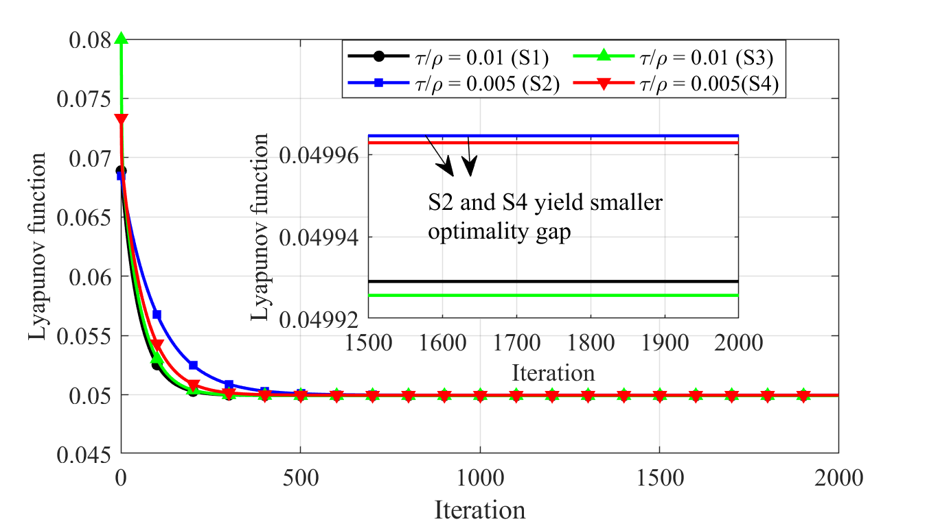
Before running the algorithm, we first can easily verify the convergence condition (C1) stated in Theorem 1 for S1-S4. We use the interior-point method embedded in the fmincon solver of MATLAB to solve subproblems (6). We run Algorithm 1 sufficiently long (i.e., $K=2000$ iterations when the Lyapunov function does not change apparently) for the settings S1-S4. We first examine the convergence of the method indicated by the Lyapunov function. Fig. 1 (a) shows the evolution of the Lyapunov function w.r.t. the iterations with S1-S4. We observe that for all the settings S1-S4, the Lyapunov functions strictly decrease w.r.t. the iterations and finally stabilize at some value that is close to the optima $f^{\star}=0.1x_{1}^{\star}+0.1x_{2}^{\star}+0.1x_{1}^{\star}x_{2}^{\star}=0.05$ . By further examining the results, we note that a larger ratio $\tau/\rho$ yields faster convergence rate as with S1/S3 ( $\tau/\rho=0.01$ ) compared with S2/S4 ( $\tau/\rho=0.005$ ). This is caused by the relatively smaller penalty factor $\rho$ and proximal factor $\beta$ required to ensure the convergence condition (C1) for a larger $\tau/\rho$ . Note that the penalty factor $\rho$ and the proximal factor $\beta$ can be interpreted as some means to slow down the primal updates as they have an effect in penalizing the deviation from current update $\mathbf{x}^{k}$ . Oppositely, a smaller ratio $\tau/\rho$ generally yields higher solution quality (i.e., smaller suboptimality gap) as with S2/S4 ( $\tau/\rho=0.005$ ) compared with S1/S3 ( $\tau/\rho=0.01$ ). This is in line with Theorem 1.

To further examine the solution quality, we report the detailed results with the four settings S1-S4 (Prox-ADMM-Sx, x = 1, 2, 3, 4) and the centralized method (using the interior-point method embedded in the fmincon solver of MATLAB) in Table 2. Note that the convergent solution $\hat{x}_{1}$ and $\hat{x}_{2}$ with proximal ADMM under the settings S1-S4 are quite close to the optimal solution $x^{\star}_{1}=0.5$ and $x_{2}^{\star}=0.5$ obtained from the centralized method. More specifically, by measuring the sub-optimality by $\|\hat{\mathbf{x}}-\mathbf{x}^{\star}\|/\|\mathbf{x}^{\star}\|$ where $\hat{\mathbf{x}}=(\hat{x}_{1},\hat{x}_{2})$ and $\mathbf{x}^{\star}=(x_{1}^{\star},x_{2}^{\star})$ are the convergent and optimal solution, we have the sub-optimality of proximal ADMM is around 1.2E-3 with S1/S3 ( $\tau/\rho=0.01$ ) and 5.9E-4 with S2/S4 ( $\tau/\rho=0.005$ ). We therefore imply that a smaller ratio $\tau/\rho$ can achieve higher solution quality but generally at the cost of slower convergence rate as observed in Fig. 1 (a). This implies that a trade-off in terms of the solution quality and the convergence speed is necessary while configuring the algorithm (i.e., the ratio of $\tau/\rho$ ) for specific applications. For this example, considering both the solution quality and convergence rate, we have S4 a preferred option. We therefore display the convergence of primal variables $x_{1}$ and $x_{2}$ with S4 in Fig. 1(b). Note that $x_{1}$ and $x_{2}$ gradually approach the optimal solution $\mathbf{x}_{1}^{\star}=0.5$ and $x_{2}^{\star}=0.5$ .

Table 2: Performance of proximal ADMM under the settings S1-S4 vs. Centralized method

Method	$\tau/\rho$	$\hat{x}_{1}$	$\hat{x}_{2}$	Sub- optimality	Convergence Rate
Centralized	–	0.5	0.5	–	–
Prox-ADMM-S1	0.01	0.4994	0.4994	1.1E-3	No. 1
Prox-ADMM-S2	0.005	0.4997	0.4997	5.7E-4	No. 4
Prox-ADMM-S3	0.01	0.4994	0.4994	1.2E-3	No .2
Prox-ADMM-S4	0.005	0.4997	0.4997	5.9E-4	No. 3

Refer to caption — Figure 1: (a) The evolution of Lyapunov function $T_{c}^{k}$ with S1-S4. (b) The evolution of primal variables $x_{1}$ and $x_{2}$ with S4.

4.2 Application: multi-zone HVAC control

To showcase the performance of proximal ADMM in applications, we apply it to the multi-zone heating, ventilation, and air conditioning (HVAC) control arising from smart buildings [7, 6, yang2021stochastic]. The goal is to optimize the HVAC operation to provide the comfortable temperature with minimal electricity bill. Due to the thermal capacity of buildings, the evolution of indoor temperature is a slow process affected both by the dynamic indoor occupancy (thermal loads) and the HVAC operation (cooling loads). The general solution is to design a model predictive controller for optimizing HVAC operation (i.e., zone mass flow and zone temperature trajectories) to minimize the overall electricity cost while respecting the comfortable temperature ranges based on the predicted information (i.e., indoor occupancy, outdoor temperature, electricity price, etc.). The general problem formulation is presented below.


$\displaystyle\min_{\mathbf{m}^{z},\mathbf{T}}$	$\displaystyle\sum_{t}c_{t}\big\{c_{p}(1-d_{r})\sum_{i}m^{zi}_{t}(T^{o}_{t}-T^{c})$	( $\mathbf{P2}$ )
	$\displaystyle+c_{p}\eta d_{r}\sum_{i}m^{zi}_{t}(T^{i}_{t}-T^{c})+\kappa_{f}\big(\textstyle\sum_{i}{m^{zi}_{t}}\big)^{2}\big\}\Delta_{t}$
s.t.	$\displaystyle~T^{i}_{t+1}=A_{ii}T^{i}_{t}+{\textstyle\sum}_{j\in N_{i}}A_{ij}T^{j}_{t}$
	$\displaystyle\hskip 9.24994pt\hskip 9.24994pt\hskip 9.24994pt+C_{ii}m^{zi}_{t}(T^{i}_{t}-T^{c})+D^{i}_{t},~\forall i,t.$	(14a)
	$\displaystyle{T}^{i}_{\min}\leq T^{i}_{t}\leq T^{i}_{\max},~~~~\forall i,t.$	(14b)
	$\displaystyle m^{zi}_{\min}\leq m^{zi}_{t}\leq m^{zi}_{\max},~\forall i,t.$	(14c)
	$\displaystyle\textstyle\sum_{i}m^{zi}_{t}\leq\overline{m},~\forall t.$	(14d)

where $i$ and $t$ are zone and time indices, $\mathbf{T}=(T^{i}_{t})_{\forall i,t}$ and $\mathbf{m}^{z}=(m^{zi}_{t})_{\forall i,t}$ are zone temperature and the supplied zone mass flow rates, which are decision variables. Note that we have the HVAC system serves $N$ zones with thermal couplings (i.e., heat transfer) within a building. The other notations are parameters. For example, $[T^{i}_{\min},T^{i}_{\max}]$ represent the comfortable temperature range of zone $i$ . The problem is subject to the constraints including zone thermal couplings (14a), comfortable temperature margins (14b), zone mass flow rate limits (14c), and total zone mass flow rate limits (14d).

Note that problem ( P2 ) is generally in large scale for a commercial building due to the large number of zones and rooms. This problem represents one of the major challenging problems with smart buildings. Centralized strategies are generally not suitable due to the computation and communication overheads. In this part, we show how the proximal ADMM can be applied to solve problem ( P2 ) in a distributed manner and thus overcome the computation burden. We first reformulate problem ( P2 ) as ( P3 ). We have


		$\displaystyle\min_{\mathbf{m}^{z},\mathbf{T}}\sum_{t}c_{t}\big\{c_{p}(1-d_{r})\sum_{i}m^{zi}_{t}(T^{o}_{t}-T^{c})$		( $\mathbf{P3}$ )
		$\displaystyle+c_{p}\eta d_{r}\sum_{i}m^{zi}_{t}(T^{ii}_{t}-T^{c})+\kappa_{f}\big(\textstyle\sum_{i}{m^{zi}_{t}}\big)^{2}\big\}\Delta_{t}$
		$\displaystyle+M\textstyle\sum_{i}\textstyle\sum_{t}\big(T^{ii}_{t+1}-A_{ii}T^{ii}_{t}-{\sum}_{j\in N_{i}}A_{ij}T^{ij}_{t}$
		$\displaystyle\hskip 9.24994pt\hskip 9.24994pt-C_{ii}m^{zi}_{t}(T^{ii}_{t}-T^{c})-D^{i}_{t}\big)^{2}$
		$\displaystyle\text{s.t.}~~T^{ij}_{t}=\overline{T}^{j}_{t},~~\forall i,j,t.$		(15a)
		$\displaystyle\hskip 9.24994pt\hskip 9.24994ptT^{i}_{\min}\leq T^{ii}_{t}\leq T^{i}_{\max},~~~\forall i,t.$		(15b)
		$\displaystyle\hskip 9.24994pt\hskip 9.24994ptT^{i}_{\min}\leq\overline{T}^{i}_{t}\leq T^{i}_{\max},~~~\forall i,t.$		(15c)
		$\displaystyle\hskip 9.24994pt\hskip 9.24994ptm^{zi}_{\min}\leq m^{zi}_{t}\leq m^{zi}_{\max},~~~\forall i,t.$		(15d)
		$\displaystyle\hskip 9.24994pt\hskip 9.24994pt\textstyle\sum_{i}m^{zi}_{t}\leq\overline{m},~\forall t.$		(15e)

where we have augmented the decision variables for each zone controller to involve the copy of temperature for its neighboring zones, i.e., $\mathbf{T}^{i}:=(T^{ij}_{t})_{j\in N_{i},~t}$ with $T^{ij}_{t}$ denoting the estimated temperature of zone $j$ by zone $i$ and $N_{i}$ representing the neighboring zones of zone $i$ . Besides, to drive the consistence of duplicated zone temperature copies, we introduce a block of consensus variable $\overline{\mathbf{T}}=(\overline{T}^{i}_{t})_{i,t}$ . Considering the challenging to handle the hard non-linear constraints (14a), we turn to the penalty method and penalize the violations by quadratic terms. Note that problem ( P3 ) fits into the template ( P ) and we have $N+1$ computing agents, where agents $1$ to $N$ correspond to the zones with the augmented decision variable $\mathbf{x}_{i}=((T^{ij}_{t})_{j\in N_{i},t},(m^{zi}_{t})_{t})$ , and agent $0$ control the consensus decision variable $\overline{\mathbf{T}}=(\overline{T}_{i})_{i\in N}$ . Constraints (15a) and (15e) represents the coupled linear constraints which can be expressed in the compact form $\mathbf{A}\mathbf{x}=\mathbf{b}$ if necessary. The other constraints comprise the local bounded convex constraints $\mathbf{X}_{i}$ for the agents.

We consider a case study with $N=10$ zones and the predicted horizon $T=48$ time slots (a whole day with a sampling interval of 30 $\mathrm{m}\mathrm{i}\mathrm{n}\mathrm{s}$ ). We set the lower and upper comfortable temperature bounds as $T^{i}_{\min}=24^{\circ}$ C and $T^{i}_{\max}=26^{\circ}$ C. The specifications for HVAC system can refer to [6, 7]. The algorithm of proximal ADMM is configured by $\rho=2.0$ , $\tau=0.1$ , $\beta=3.0$ , $\mathbf{B}_{i}=\mathbf{I}$ (suitable sizes), and $c=8.7$ . We run the algorithm suitably long ( $K=200$ iterations when both the residual and Lyapunov function do not change apparently). We first examine the convergence of the algorithm measured by the Lyapunov function and the norm of (coupled) constraints residual. We visualize the Lyapunov function and constraints residual in Fig. 2. Note that the Lyapunov function strictly declines along the iterations, which is consistent with our theoretical analysis. Besides, the constraints residual almost strictly decreases with the iterations as well and finally approaches zero. We have the overall norm of the constraints residual at the end of iterations is about $0.38$ , which is quite small considering the problem scale $T\cdot N=480$ . This justifies the convergence property of proximal ADMM for the smart building application.

We next evaluate the solution quality measured by the HVAC electricity cost and human comfort. We randomly pick $3$ zones (zone 1, 3, 7) and display the predicted zone occupancy (inputs), the zone mass flow rates (zone MFR, control variables) , and the zone temperature (zone temp., control variables) over the $48$ time slots in Fig. 3. Note that the variations of zone MFR are almost consistent with the zone occupancy. This is reasonable as the zone occupancy determines the thermal loads which need to be balanced by the zone mass flow rates. We besides see that the zone temp. are all maintained within the comfortable range $[24,26]^{\circ}$ C. This infers the satisfaction of human comfort. To further evaluate the solution quality and computation efficiency, we compare the proximal ADMM (Prox-ADMM) with centralized method (Centralized). Specifically, we use the interior-point embedded in the fmincon solver of MATLAB to solve both the subproblems (6) with Prox-ADMM and problem ( P2 ) with Centralized. For the Centralized, we run the solver sufficiently long without considering the time with the objective to approach the best possible optimal solution. We compare the two methods in three folds, i.e., electricity cost, the norm of constraints residual, and computation time as reported in Table 3. We see that electricity cost with Prox-ADMM is about $160.20$ (s$) versus $153.12$ (s$) yield by Centralized. We imply the sub-optimality of Prox-ADMM in terms of the objective is about $5.0\%$ . However, the Prox-ADMM obviously outperforms the Centralized in computation efficiency. The average computing time for each zone is about 50 $\mathrm{m}\mathrm{i}\mathrm{n}$ with Prox-ADMM (parallel computation) while the Centralized takes more than 10 $\mathrm{h}$ . Note that we have picked $T=48$ time slots (a whole day) as the predicted horizon, the computing time could be largely sharpened in practice with a much smaller prediction horizon, say $T=10$ time slots (5 $\mathrm{h}$ ).

Table 3: Prox-ADMM vs. Centralized for HVAC control in smart buildings (

N=10

zones)

Method	Electricity cost (s$)	Human comfort	Constraints residual	Computing time
Centralized	153.12	Y	0	$\geq 10$ $\mathrm{h}$
Prox-ADMM	160.54	Y	0.38	50 $\mathrm{min}$

5 Conclusion and Future Work

This paper focused on developing a distributed algorithm for a class of nonconvex and nonsmooth problems with convergence guarantee. The problems are featured by i) a possibly nonconvex objective composed of both separate and composite components, ii) local bounded convex constraints, and iii) global coupled linear constraints. This class of problems is broad in application but lacks distributed methods with convergence guarantee. We turned to the powerful alternating direction method of multiplier (ADMM) for constrained optimization but faced the challenge to establish convergence. Noting that the underlying obstacle is to assume the boundness of dual updates, we revised the classic ADMM and proposed to update the dual variables in a distributed manner. This leads to a proximal ADMM with the convergence guarantee towards the approximate stationary points of the problem. We demonstrated the convergence and solution quality of the distributed method by a numerical example and a concrete application to the multi-zone heating, ventilation, and air-condition (HVAC) control arising from smart buildings.

This paper proposed the discounted dual update scheme in conjunction with ADMM for a class of nonconvex and nonsmooth problems, some interesting future work includes studying whether the discounted dual update scheme can be explored to develop distributed methods for more broad classes of problems both in convex and nonconvex settings.

References

[1] W. Shi, Q. Ling, K. Yuan, G. Wu, and W. Yin, “On the linear convergence of the ADMM in decentralized consensus optimization,” IEEE Transactions on Signal Processing, vol. 62, no. 7, pp. 1750–1761, 2014.
[2] W. Deng, M.-J. Lai, Z. Peng, and W. Yin, “Parallel multi-block ADMM with O (1/k) convergence,” Journal of Scientific Computing, vol. 71, no. 2, pp. 712–736, 2017.
[3] A. Falsone, I. Notarnicola, G. Notarstefano, and M. Prandini, “Tracking-ADMM for distributed constraint-coupled optimization,” Automatica, vol. 117, p. 108962, 2020.
[4] B. Houska, J. Frasch, and M. Diehl, “An augmented lagrangian based algorithm for distributed nonconvex optimization,” SIAM Journal on Optimization, vol. 26, no. 2, pp. 1101–1127, 2016.
[5] Y. Wang, W. Yin, and J. Zeng, “Global convergence of ADMM in nonconvex nonsmooth optimization,” Journal of Scientific Computing, vol. 78, no. 1, pp. 29–63, 2019.
[6] Y. Yang, G. Hu, and C. J. Spanos, “HVAC energy cost optimization for a multizone building via a decentralized approach,” IEEE Transactions on Automation Science and Engineering, vol. 17, no. 4, pp. 1950–1960, 2020.
[7] Y. Yang, S. Srinivasan, G. Hu, and C. J. Spanos, “Distributed Control of Multizone HVAC Systems Considering Indoor Air Quality,” IEEE Transactions on Control Systems Technology, 2021.
[8] J. A. Ansere, G. Han, L. Liu, Y. Peng, and M. Kamal, “Optimal resource allocation in energy-efficient internet-of-things networks with imperfect CSI,” IEEE Internet of Things Journal, vol. 7, no. 6, pp. 5401–5411, 2020.
[9] Y. Yang, G. Hu, and C. J. Spanos, “Optimal sharing and fair cost allocation of community energy storage,” IEEE Transactions on Smart Grid, vol. 12, no. 5, pp. 4185–4194, 2021.
[10] Y. Yang, U. Agwan, G. Hu, and C. J. Spanos, “Selling renewable utilization service to consumers via cloud energy storage,” arXiv preprint arXiv:2012.14650.
[11] L. Zhang, V. Kekatos, and G. B. Giannakis, “Scalable electric vehicle charging protocols,” IEEE Transactions on Power Systems, vol. 32, no. 2, pp. 1451–1462, 2016.
[12] Y. Yang, Q.-S. Jia, X. Guan, X. Zhang, Z. Qiu, and G. Deconinck, “Decentralized ev-based charging optimization with building integrated wind energy,” IEEE Transactions on Automation Science and Engineering, vol. 16, no. 3, pp. 1002–1017, 2018.
[13] Y. Yang, Q.-S. Jia, G. Deconinck, X. Guan, Z. Qiu, and Z. Hu, “Distributed coordination of ev charging with renewable energy in a microgrid of buildings,” IEEE Transactions on Smart Grid, vol. 9, no. 6, pp. 6253–6264, 2017.
[14] Y. Yang, Q.-S. Jia, and X. Guan, “Stochastic coordination of aggregated electric vehicle charging with on-site wind power at multiple buildings,” in 2017 IEEE 56th Annual Conference on Decision and Control (CDC), pp. 4434–4439, IEEE, 2017.
[15] Y. Yang, Q.-S. Jia, and X. Guan, “The joint scheduling of ev charging load with building mounted wind power using simulation-based policy improvement,” in 2016 International Symposium on Flexible Automation (ISFA), pp. 165–170, IEEE, 2016.
[16] T. Long, Q.-S. Jia, G. Wang, and Y. Yang, “Efficient real-time ev charging scheduling via ordinal optimization,” IEEE Transactions on Smart Grid, vol. 12, no. 5, pp. 4029–4038, 2021.
[17] Y. Yang, Y. Chen, G. Hu, and C. J. Spanos, “Optimal network charge for peer-to-peer energy trading: A grid perspective,” arXiv preprint arXiv:2205.01945, 2022.
[18] Y. Chen, Y. Yang, and X. Xu, “Towards transactive energy: An analysis of information-related practical issues,” Energy Conversion and Economics, vol. 3, no. 3, pp. 112–121, 2022.
[19] M. K. Arpanahi, M. H. Golshan, and P. Siano, “A Comprehensive and Efficient Decentralized Framework for Coordinated Multiperiod Economic Dispatch of Transmission and Distribution Systems,” IEEE Systems Journal, 2020.
[20] S. Hashempour, A. A. Suratgar, and A. Afshar, “Distributed Nonconvex Optimization for Energy Efficiency in Mobile Ad Hoc Networks,” IEEE Systems Journal, 2021.
[21] I. Necoara and V. Nedelcu, “On linear convergence of a distributed dual gradient algorithm for linearly constrained separable convex problems,” Automatica, vol. 55, pp. 209–216, 2015.
[22] A. Falsone, K. Margellos, S. Garatti, and M. Prandini, “Dual decomposition for multi-agent distributed optimization with coupling constraints,” Automatica, vol. 84, pp. 149–158, 2017.
[23] S. Boyd, N. Parikh, and E. Chu, Distributed optimization and statistical learning via the alternating direction method of multipliers. Now Publishers Inc, 2011.
[24] T.-Y. Lin, S.-Q. Ma, and S.-Z. Zhang, “On the sublinear convergence rate of multi-block ADMM,” Journal of the Operations Research Society of China, vol. 3, no. 3, pp. 251–274, 2015.
[25] X. Cai, D. Han, and X. Yuan, “On the convergence of the direct extension of ADMM for three-block separable convex minimization models with one strongly convex function,” Computational Optimization and Applications, vol. 66, no. 1, pp. 39–73, 2017.
[26] J. Bai, J. Li, F. Xu, and H. Zhang, “Generalized symmetric ADMM for separable convex optimization,” Computational optimization and applications, vol. 70, no. 1, pp. 129–170, 2018.
[27] N. Chatzipanagiotis and M. M. Zavlanos, “On the convergence of a distributed augmented lagrangian method for nonconvex optimization,” IEEE Transactions on Automatic Control, vol. 62, no. 9, pp. 4405–4420, 2017.
[28] N. S. Aybat, Z. Wang, T. Lin, and S. Ma, “Distributed linearized alternating direction method of multipliers for composite convex consensus optimization,” IEEE Transactions on Automatic Control, vol. 63, no. 1, pp. 5–20, 2017.
[29] J. Bai, W. W. Hager, and H. Zhang, “An inexact accelerated stochastic ADMM for separable convex optimization,” Computational Optimization and Applications, pp. 1–40, 2022.
[30] L. Yang, T. K. Pong, and X. Chen, “Alternating direction method of multipliers for a class of nonconvex and nonsmooth problems with applications to background/foreground extraction,” SIAM Journal on Imaging Sciences, vol. 10, no. 1, pp. 74–110, 2017.
[31] K. Guo, D. Han, and T.-T. Wu, “Convergence of alternating direction method for minimizing sum of two nonconvex functions with linear constraints,” International Journal of Computer Mathematics, vol. 94, no. 8, pp. 1653–1669, 2017.
[32] G. Li and T. K. Pong, “Global convergence of splitting methods for nonconvex composite optimization,” SIAM Journal on Optimization, vol. 25, no. 4, pp. 2434–2460, 2015.
[33] Q. Liu, X. Shen, and Y. Gu, “Linearized ADMM for nonconvex nonsmooth optimization with convergence analysis,” IEEE Access, vol. 7, pp. 76131–76144, 2019.
[34] M. Hong, Z.-Q. Luo, and M. Razaviyayn, “Convergence analysis of alternating direction method of multipliers for a family of nonconvex problems,” SIAM Journal on Optimization, vol. 26, no. 1, pp. 337–364, 2016.
[35] K. Sun and X. A. Sun, “A two-level distributed algorithm for general constrained non-convex optimization with global convergence,” arXiv preprint arXiv:1902.07654, 2019.
[36] K. Sun and X. A. Sun, “A two-level ADMM algorithm for AC OPF with convergence guarantees,” IEEE Transactions on Power Systems, 2021.
[37] Y. Yang, G. Hu, and C. J. Spanos, “A proximal linearization-based decentralized method for nonconvex problems with nonlinear constraints,” arXiv preprint arXiv:2001.00767, 2020.
[38] Y. Yang, X. Guan, Q.-S. Jia, L. Yu, B. Xu, and C. J. Spanos, “A survey of admm variants for distributed optimization: Problems, algorithms and features,” arXiv preprint arXiv:2208.03700, 2022.
[39] X. Li, G. Feng, and L. Xie, “Distributed proximal algorithms for multiagent optimization with coupled inequality constraints,” IEEE Transactions on Automatic Control, vol. 66, no. 3, pp. 1223–1230, 2020.
[40] T.-H. Chang, M. Hong, and X. Wang, “Multi-agent distributed optimization via inexact consensus ADMM,” IEEE Transactions on Signal Processing, vol. 63, no. 2, pp. 482–497, 2014.
[41] S. Lu, J. D. Lee, M. Razaviyayn, and M. Hong, “Linearized ADMM converges to second-order stationary points for non-convex problems,” IEEE Transactions on Signal Processing, vol. 69, pp. 4859–4874, 2021.
[42] P. Jain and P. Kar, “Non-convex optimization for machine learning,” 2017.
[43] H. Li and Z. Lin, “Accelerated proximal gradient methods for nonconvex programming,” Advances in neural information processing systems, vol. 28, 2015.

Appendix A Proof of Proposition 1

Prop. 1 is established based on the first-order optimality condition of subproblems (6) and the $\Lips$ continuous gradient property of $f$ and $g$ .

We first establish the following equality and notation.

		$\displaystyle\mathbf{A}_{i}\mathbf{x}^{k+1}_{i}+{\textstyle\sum}_{j\neq i}\mathbf{A}_{j}\mathbf{x}^{k}_{j}-\mathbf{b}$		(16)
		$\displaystyle~=\!\mathbf{A}\mathbf{x}^{k}-\mathbf{b}+\mathbf{A}_{i}(\mathbf{x}_{i}^{k+1}-\mathbf{x}_{i}^{k}).$
		$\displaystyle~=\!\mathbf{A}\mathbf{x}^{k+1}\!-\!\mathbf{b}+\mathbf{A}(\mathbf{x}^{k}-\mathbf{x}^{k+1})+\mathbf{A}_{i}(\mathbf{x}_{i}^{k+1}-\mathbf{x}_{i}^{k}).$
		$\displaystyle\hat{\bm{\lambda}}^{k}:=\bm{\lambda}^{k}+\rho(\mathbf{A}\mathbf{x}^{k+1}-\mathbf{b}).$		(17)

For subproblems (6), the first-order optimality condition states that there exists $\nu_{i}^{k+1}\in N_{\mathbf{X}_{i}}(\mathbf{x}_{i}^{k+1})$ that

	$\displaystyle 0$	$\displaystyle=~\nabla f_{i}(\mathbf{x}_{i}^{k+1})+\nabla_{i}g(\mathbf{x}^{k})+\mathbf{A}^{\top}_{i}\bm{\lambda}^{k}$
		$\displaystyle\hskip 9.24994pt\hskip 9.24994pt+\rho\mathbf{A}^{\top}_{i}(\mathbf{A}_{i}\mathbf{x}^{k+1}_{i}+{\textstyle\sum}_{j\neq i}\mathbf{A}_{j}\mathbf{x}^{k}_{j}-\mathbf{b})$
		$\displaystyle\hskip 9.24994pt\hskip 9.24994pt+\beta\mathbf{B}^{\top}_{i}\mathbf{B}_{i}(\mathbf{x}^{k+1}_{i}-\mathbf{x}^{k}_{i})+\nu_{i}^{k+1}$
		$\displaystyle=~\nabla f_{i}(\mathbf{x}_{i}^{k+1})+\nabla_{i}g(\mathbf{x}^{k})+\mathbf{A}^{\top}_{i}\big(\bm{\lambda}^{k}+\rho(\mathbf{A}\mathbf{x}^{k+1}-\mathbf{b})\big)$
		$\displaystyle\hskip 9.24994pt\hskip 9.24994pt+\rho\mathbf{A}_{i}^{\top}\mathbf{A}(\mathbf{x}^{k}-\mathbf{x}^{k+1})+\rho\mathbf{A}_{i}^{\top}\mathbf{A}_{i}(\mathbf{x}_{i}^{k+1}-\mathbf{x}_{i}^{k})$
		$\displaystyle\hskip 9.24994pt\hskip 9.24994pt+\beta\mathbf{B}^{\top}_{i}\mathbf{B}_{i}(\mathbf{x}^{k+1}_{i}-\mathbf{x}^{k}_{i})+\nu_{i}^{k+1}~~~~~~~~~~\text{by }\eqref{eq:equality}$
		$\displaystyle=~\nabla f_{i}(\mathbf{x}_{i}^{k+1})+\nabla_{i}g(\mathbf{x}^{k})+\mathbf{A}^{\top}_{i}\hat{\bm{\lambda}}^{k}+\rho\mathbf{A}^{\top}_{i}\mathbf{A}(\mathbf{x}^{k}-\mathbf{x}^{k+1})$
		$\displaystyle\hskip 9.24994pt\hskip 9.24994pt+\rho\mathbf{A}^{\top}_{i}\mathbf{A}_{i}(\mathbf{x}_{i}^{k+1}-\mathbf{x}_{i}^{k})$
		$\displaystyle\hskip 9.24994pt\hskip 9.24994pt+\beta\mathbf{B}^{\top}_{i}\mathbf{B}_{i}\big(\mathbf{x}^{k+1}_{i}-\mathbf{x}^{k}_{i}\big)+\nu_{i}^{k+1}~~~~~~~~~~\text{by}~\eqref{eq:hatlambda}.$

Multiplying by ( $\mathbf{x}_{i}^{k+1}-\mathbf{x}_{i}$ ) in both sides, we have

\begin{split}&\langle\nabla f_{i}(\mathbf{x}_{i}^{k+1}),\mathbf{x}_{i}^{k+1}-\mathbf{x}_{i}\rangle+\langle\nabla_{i}g(\mathbf{x}^{k}),\mathbf{x}_{i}^{k+1}-\mathbf{x}_{i}\rangle\\ &+\langle\hat{\bm{\lambda}}^{k},\mathbf{A}_{i}(\mathbf{x}_{i}^{k+1}-\mathbf{x}_{i})\rangle\\ &+\rho\langle\mathbf{A}(\mathbf{x}^{k}-\mathbf{x}^{k+1}),\mathbf{A}_{i}(\mathbf{x}_{i}^{k+1}-\mathbf{x}_{i})\rangle\\ \ &+\rho\langle\mathbf{A}_{i}(\mathbf{x}_{i}^{k+1}-\mathbf{x}_{i}^{k}),\mathbf{A}_{i}(\mathbf{x}_{i}^{k+1}-\mathbf{x}_{i})\rangle\\ &+\beta\langle\mathbf{B}_{i}(\mathbf{x}^{k+1}_{i}-\mathbf{x}^{k}_{i}),\mathbf{B}_{i}(\mathbf{x}_{i}^{k+1}-\mathbf{x}_{i})\rangle\\ =&-\langle\nu_{i}^{k+1},\mathbf{x}_{i}^{k+1}-\mathbf{x}_{i}\rangle\leq 0,~~\forall\mathbf{x}_{i}\in\mathbf{X}_{i}.\end{split}

(18)

Summing up (18) over $i$ , we have $\forall\mathbf{x}_{i}\in\mathbf{X}_{i}$ ,

	$\displaystyle\langle\nabla$	$\displaystyle f(\mathbf{x}^{k+1}),\mathbf{x}^{k+1}-\mathbf{x}\rangle+\langle\nabla g(\mathbf{x}^{k}),\mathbf{x}^{k+1}-\mathbf{x}\rangle$
		$\displaystyle+\langle\hat{\bm{\lambda}}^{k},\mathbf{A}(\mathbf{x}^{k+1}-\mathbf{x})\rangle+(\mathbf{x}^{k+1}-\mathbf{x})\rho\mathbf{A}^{\top}\mathbf{A}(\mathbf{x}^{k}-\mathbf{x}^{k+1})$
		$\displaystyle+\textstyle\sum_{i}(\mathbf{x}^{k+1}_{i}-\mathbf{x}_{i})^{\top}(\rho\mathbf{A}^{\top}_{i}\mathbf{A}_{i}+\beta\mathbf{B}^{\top}_{i}\mathbf{B}_{i})(\mathbf{x}^{k+1}_{i}-\mathbf{x}^{k}_{i})\leq 0.$

Plugging in $\mathbf{Q}:=\rho G_{\mathbf{A}}+\beta G_{\mathbf{B}}-\rho\mathbf{A}^{\top}\mathbf{A}$ , we have

$\displaystyle\langle\nabla$	$\displaystyle f(\mathbf{x}^{k+1}),\mathbf{x}^{k+1}-\mathbf{x}\rangle+\langle\nabla g(\mathbf{x}^{k}),\mathbf{x}^{k+1}-\mathbf{x}\rangle$
	$\displaystyle+\langle\hat{\bm{\lambda}}^{k},\mathbf{A}(\mathbf{x}^{k+1}-\mathbf{x})\rangle$
	$\displaystyle+(\mathbf{x}^{k+1}-\mathbf{x})^{\top}\mathbf{Q}(\mathbf{x}^{k+1}-\mathbf{x}^{k})\leq 0,~~\forall\mathbf{x}\in\mathbf{X}.$	(19)

By induction, we have

$\displaystyle\langle\nabla$	$\displaystyle f(\mathbf{x}^{k}),\mathbf{x}^{k}-\mathbf{x}\rangle+\langle\nabla g(\mathbf{x}^{k-1}),\mathbf{x}^{k}-\mathbf{x}\rangle$
	$\displaystyle+\langle\hat{\bm{\lambda}}^{k-1},\mathbf{A}(\mathbf{x}^{k}-\mathbf{x})\rangle$
	$\displaystyle+(\mathbf{x}^{k}-\mathbf{x})^{\top}\mathbf{Q}(\mathbf{x}^{k}-\mathbf{x}^{k-1})\leq 0,~~\forall\mathbf{x}\in\mathbf{X}.$	(20)

By setting $\mathbf{x}=\mathbf{x}^{k}$ and $\mathbf{x}=\mathbf{x}^{k+1}$ with (A) and (A), we have

$\displaystyle\langle\nabla$	$\displaystyle f(\mathbf{x}^{k+1}),\mathbf{x}^{k+1}-\mathbf{x}^{k}\rangle+\langle\nabla g(\mathbf{x}^{k}),\mathbf{x}^{k+1}-\mathbf{x}^{k}\rangle$
	$\displaystyle+\langle\hat{\bm{\lambda}}^{k},\mathbf{A}(\mathbf{x}^{k+1}-\mathbf{x}^{k})\rangle$
	$\displaystyle+(\mathbf{x}^{k+1}-\mathbf{x}^{k})^{\top}\mathbf{Q}(\mathbf{x}^{k+1}-\mathbf{x}^{k})\leq 0.$	(21)
$\displaystyle\langle\nabla$	$\displaystyle f(\mathbf{x}^{k}),\mathbf{x}^{k}-\mathbf{x}^{k+1}\rangle+\langle\nabla g(\mathbf{x}^{k-1}),\mathbf{x}^{k}-\mathbf{x}^{k+1}\rangle$
	$\displaystyle+\langle\hat{\bm{\lambda}}^{k-1},\mathbf{A}(\mathbf{x}^{k}-\mathbf{x}^{k+1})\rangle$
	$\displaystyle+(\mathbf{x}^{k}-\mathbf{x}^{k+1})^{\top}\mathbf{Q}(\mathbf{x}^{k}-\mathbf{x}^{k-1})\leq 0.$	(22)

Summing up (21) and (22) and plugging in $\mathbf{w}^{k}:=(\mathbf{x}^{k+1}-\mathbf{x}^{k})-(\mathbf{x}^{k}-\mathbf{x}^{k-1})$ , we have

\begin{split}\langle\nabla&f(\mathbf{x}^{k+1})-\nabla f(\mathbf{x}^{k}),\mathbf{x}^{k+1}-\mathbf{x}^{k}\rangle\\ &+\langle\nabla g(\mathbf{x}^{k})-\nabla g(\mathbf{x}^{k-1}),\mathbf{x}^{k+1}-\mathbf{x}^{k}\rangle\\ &+\langle\hat{\bm{\lambda}}^{k}-\hat{\bm{\lambda}}^{k-1},\mathbf{A}(\mathbf{x}^{k+1}-\mathbf{x}^{k})\rangle\\ &+(\mathbf{x}^{k+1}-\mathbf{x}^{k})^{\top}\mathbf{Q}\mathbf{w}^{k}\leq 0.\end{split}

(23)

Based on the $\Lips$ continuous gradient property of $f$ over the compact set $\mathbf{x}\in\mathbf{X}$ , we have

\begin{split}\langle\nabla f(\mathbf{x}^{k+1})\!-\!\nabla f(\mathbf{x}^{k}),\mathbf{x}^{k+1}\!-\!\mathbf{x}^{k}\rangle\!\geq\!-L_{f}\|\mathbf{x}^{k+1}\!-\!\mathbf{x}^{k}\|^{2}.\end{split}

(24)

We also have

		$\displaystyle\langle\nabla g(\mathbf{x}^{k})-\nabla g(\mathbf{x}^{k-1}),\mathbf{x}^{k+1}-\mathbf{x}^{k}\rangle$
		$\displaystyle=\langle\frac{\nabla g(\mathbf{x}^{k})-\nabla g(\mathbf{x}^{k-1})}{\sqrt{L_{g}}},\sqrt{L_{g}}(\mathbf{x}^{k+1}-\mathbf{x}^{k})\rangle$
		$\displaystyle\geq-\frac{1}{2L_{g}}\\|\nabla g(\mathbf{x}^{k})-\nabla g(\mathbf{x}^{k-1})\\|^{2}-\frac{L_{g}}{2}\\|\mathbf{x}^{k+1}-\mathbf{x}^{k}\\|^{2}$
		$\displaystyle\geq-\frac{L_{g}}{2}\\|\mathbf{x}^{k}-\mathbf{x}^{k-1}\\|^{2}-\frac{L_{g}}{2}\\|\mathbf{x}^{k+1}-\mathbf{x}^{k}\\|^{2}$

where the last equality is based on the $\Lips$ continuous gradient property of $g$ .

Besides, we have

\begin{split}&\hskip 9.24994pt\langle\hat{\bm{\lambda}}^{k}-\hat{\bm{\lambda}}^{k-1},\mathbf{A}(\mathbf{x}^{k+1}-\mathbf{x}^{k})\rangle\\ &=\left\langle\bm{\lambda}^{k+1}-\bm{\lambda}^{k}+\tau(\bm{\lambda}^{k}-\bm{\lambda}^{k-1}),\mathbf{A}(\mathbf{x}^{k+1}-\mathbf{x}^{k})\right\rangle\\ &=\Big\langle\bm{\lambda}^{k+1}-\bm{\lambda}^{k}+\tau(\bm{\lambda}^{k}-\bm{\lambda}^{k-1}),\\ &\hskip 9.24994pt\hskip 9.24994pt\hskip 9.24994pt\hskip 9.24994pt\frac{\bm{\lambda}^{k+1}-\bm{\lambda}^{k}}{\rho}-\frac{(1-\tau)}{\rho}(\bm{\lambda}^{k}-\bm{\lambda}^{k-1})\Big\rangle\\ &=\frac{\|\bm{\lambda}^{k+1}\!-\!\bm{\lambda}^{k}\|^{2}}{\rho}\!-\!\frac{(1-2\tau)}{\rho}\langle\bm{\lambda}^{k+1}-\bm{\lambda}^{k},\bm{\lambda}^{k}-\bm{\lambda}^{k-1}\rangle\\ &\hskip 9.24994pt-\frac{\tau(1-\tau)}{\rho}\|\bm{\lambda}^{k}-\bm{\lambda}^{k-1}\|^{2}\\ &\geq\frac{\|\bm{\lambda}^{k+1}-\bm{\lambda}^{k}\|^{2}}{\rho}-\frac{1-2\tau}{2\rho}\|\bm{\lambda}^{k+1}-\bm{\lambda}^{k}\|^{2}\\ &\hskip 9.24994pt-\frac{1-2\tau}{2\rho}\|\bm{\lambda}^{k}-\bm{\lambda}^{k-1}\|^{2}-\frac{\tau(1-\tau)}{\rho}\|\bm{\lambda}^{k}-\bm{\lambda}^{k-1}\|^{2}\\ &=\frac{1-2\tau^{2}}{2\rho}\|\bm{\lambda}^{k+1}-\bm{\lambda}^{k}\|^{2}-\frac{1-2\tau^{2}}{2\rho}\|\bm{\lambda}^{k}-\bm{\lambda}^{k-1}\|^{2}\\ &\hskip 9.24994pt+{\tau(\tau+1)}/{\rho}\|\bm{\lambda}^{k+1}-\bm{\lambda}^{k}\|^{2}\end{split}

(25)

where the inequality is by $\langle\mathbf{a},\mathbf{b}\rangle\leq\frac{1}{2}(\|\mathbf{a}\|^{2}+\|\mathbf{b}\|^{2})$ .

Based on the inequality $\mathbf{b}^{\top}\mathbf{M}(\mathbf{b}-\mathbf{c})=\frac{1}{2}(\|\mathbf{b}-\mathbf{c}\|_{\mathbf{M}}^{2}+\|\mathbf{b}\|_{\mathbf{M}}^{2}-\|\mathbf{c}\|_{\mathbf{M}}^{2})$ , and by setting $\mathbf{M}=\mathbf{Q}$ , $\mathbf{b}=\mathbf{x}^{k+1}-\mathbf{x}^{k}$ , and $\mathbf{c}=\mathbf{x}^{k}-\mathbf{x}^{k-1}$ , we have

\begin{split}(\mathbf{x}^{k+1}-\mathbf{x}^{k})^{\top}\mathbf{Q}\mathbf{w}^{k}=&\frac{1}{2}(\|\mathbf{w}^{k}\|^{2}_{\mathbf{Q}}+\|\mathbf{x}^{k+1}-\mathbf{x}^{k}\|^{2}_{\mathbf{Q}}\\ &-\|\mathbf{x}^{k}-\mathbf{x}^{k-1}\|^{2}_{\mathbf{Q}}).\end{split}

(26)

Plugging (24), (25), (26) into (23), we have

		$\displaystyle\frac{1-2\tau^{2}}{2\rho}\left\\|\bm{\lambda}^{k+1}-\bm{\lambda}^{k}\right\\|^{2}+\frac{1}{2}\\|\mathbf{x}^{k+1}-\mathbf{x}^{k}\\|^{2}_{\mathbf{Q}}$
		$\displaystyle\hskip 9.24994pt+\frac{L_{g}}{2}\\|\mathbf{x}^{k+1}-\mathbf{x}^{k}\\|^{2}+\frac{1}{2}\\|\mathbf{w}^{k}\\|^{2}_{\mathbf{Q}}$
		$\displaystyle\leq\frac{1-2\tau^{2}}{2\rho}\left\\|\bm{\lambda}^{k}-\bm{\lambda}^{k-1}\right\\|^{2}+\frac{1}{2}\\|\mathbf{x}^{k}-\mathbf{x}^{k-1}\\|^{2}_{\mathbf{Q}}$
		$\displaystyle\hskip 9.24994pt+\frac{L_{g}}{2}\\|\mathbf{x}^{k}-\mathbf{x}^{k-1}\\|^{2}+(L_{g}+L_{f})\left\\|\mathbf{x}^{k+1}-\mathbf{x}^{k}\right\\|^{2}$
		$\displaystyle\hskip 9.24994pt-{\tau(1+\tau)}/{\rho}\\|\bm{\lambda}^{k+1}-\bm{\lambda}^{k}\\|^{2}.$

We therefore complete the proof.

Appendix B Proof of Proposition 2

Before starting the proof, we first establish the following inequalities to be used. Based on the $\Lips$ continuous gradient property of $f:\mathbf{R}^{n}\rightarrow\mathbf{R}$ over $\mathbf{x}\in\mathbf{X}$ (see (A1)), we have [31]

	$\displaystyle f(\mathbf{x}^{k+1})-f(\mathbf{x}^{k})\leq~$	$\displaystyle\langle\nabla f(\mathbf{x}^{k+1}),\mathbf{x}^{k+1}-\mathbf{x}^{k}\rangle$
		$\displaystyle+L_{f}/2\\|\mathbf{x}^{k}-\mathbf{x}^{k+1}\\|^{2}.$		(27)

Similarly, for $g:\mathbf{R}^{n}\rightarrow\mathbf{R}$ with $\Lips$ continuous gradient over $\mathbf{x}\in\mathbf{X}$ (see (A1)), we have [31]

	$\displaystyle g(\mathbf{x}^{k+1})-g(\mathbf{x}^{k})\leq~$	$\displaystyle\langle\nabla g(\mathbf{x}^{k}),\mathbf{x}^{k+1}-\mathbf{x}^{k}\rangle$
		$\displaystyle+L_{g}/2\\|\mathbf{x}^{k}-\mathbf{x}^{k+1}\\|^{2}.$		(28)

Besides, we have

	$\displaystyle~~~\frac{\rho}{2}\\|\mathbf{A}\mathbf{x}^{k+1}-\mathbf{b}\\|^{2}-\frac{\rho}{2}\\|\mathbf{A}\mathbf{x}^{k}-\mathbf{b}\\|^{2}$
$\displaystyle=$	$\displaystyle~~~\frac{\rho}{2}\left\langle\mathbf{A}(\mathbf{x}^{k+1}-\mathbf{x}^{k}),\mathbf{A}\mathbf{x}^{k+1}+\mathbf{A}\mathbf{x}^{k}-2\mathbf{b}\right\rangle$	(29)
$\displaystyle=$	$\displaystyle~~~\frac{\rho}{2}\left\langle\mathbf{A}(\mathbf{x}^{k+1}-\mathbf{x}^{k}),\mathbf{A}(\mathbf{x}^{k}-\mathbf{x}^{k+1})+2(\mathbf{A}\mathbf{x}^{k}-\mathbf{b})\right\rangle$
$\displaystyle=$	$\displaystyle-\!\frac{\rho}{2}\\|\mathbf{A}(\mathbf{x}^{k+1}\!\!-\!\!\mathbf{x}^{k})\\|^{2}\!+\!\left\langle\mathbf{A}(\mathbf{x}^{k+1}\!\!-\!\!\mathbf{x}^{k}),\rho(\mathbf{A}\mathbf{x}^{k+1}\!\!-\!\!\mathbf{b})\right\rangle.$

We next quantify the decrease of $\mathbb{L}_{\rho}(\mathbf{x},\bm{\lambda})$ with respect to (w.r.t.) the primal updates. We have

\begin{split}&\mathbb{L}_{\rho}(\mathbf{x}^{k+1},\bm{\lambda}^{k})-\mathbb{L}_{\rho}(\mathbf{x}^{k},\bm{\lambda}^{k})\\ =&~f(\mathbf{x}^{k+1})\!-\!f(\mathbf{x}^{k})+g(\mathbf{x}^{k+1})\!-\!g(\mathbf{x}^{k})+\langle\bm{\lambda}^{k},\mathbf{A}(\mathbf{x}^{k+1}-\mathbf{x}^{k})\rangle\\ &\hskip 9.24994pt+\frac{\rho}{2}\|\mathbf{A}\mathbf{x}^{k+1}-\mathbf{b}\|^{2}-\frac{\rho}{2}\|\mathbf{A}\mathbf{x}^{k}-\mathbf{b}\|^{2}\\ \leq&~\langle\nabla f(\mathbf{x}^{k+1})+\nabla g(\mathbf{x}^{k}),\mathbf{x}^{k+1}-\mathbf{x}^{k}\rangle+\rho_{F}/2\|\mathbf{x}^{k}-\mathbf{x}^{k+1}\|^{2}\\ &\hskip 9.24994pt+\left\langle\bm{\lambda}^{k},\mathbf{A}(\mathbf{x}^{k+1}-\mathbf{x}^{k})\right\rangle-\frac{\rho}{2}\|\mathbf{A}(\mathbf{x}^{k+1}-\mathbf{x}^{k})\|^{2}\\ &\hskip 9.24994pt\!+\!\left\langle\mathbf{A}(\mathbf{x}^{k+1}-\mathbf{x}^{k}),\rho(\mathbf{A}\mathbf{x}^{k+1}-\mathbf{b})\right\rangle~\text{by \eqref{eq:Lipsf}, \eqref{eq:Lipsg}, \eqref{eq:inequality2}}\\ =&~\langle\nabla f(\mathbf{x}^{k+1})+\nabla g(\mathbf{x}^{k})+\mathbf{A}^{\top}\hat{\bm{\lambda}}^{k},\mathbf{x}^{k+1}-\mathbf{x}^{k}\rangle\\ &\hskip 9.24994pt+\rho_{F}/2\|\mathbf{x}^{k}-\mathbf{x}^{k+1}\|^{2}-{\rho}/{2}\|\mathbf{A}(\mathbf{x}^{k+1}-\mathbf{x}^{k})\|^{2}~~\text{by \eqref{eq:hatlambda}}\\ \leq&-\!\|\mathbf{x}^{k+1}\!-\!\mathbf{x}^{k}\|_{\mathbf{Q}}^{2}\!+\!{\rho_{F}}/{2}\|\mathbf{x}^{k}\!-\!\mathbf{x}^{k+1}\|^{2}\!\\ &\hskip 9.24994pt-\!{\rho}/{2}~\|\mathbf{A}(\mathbf{x}^{k+1}-\mathbf{x}^{k})\|^{2}~~\text{by \eqref{eq:k}}.\\ \end{split}

(30)

We next quantify the change of $\mathbb{L}_{\rho}(\mathbf{x},\bm{\lambda})$ w.r.t. dual update. We have

\begin{split}&\mathbb{L}_{\rho}(\mathbf{x}^{k+1},\bm{\lambda}^{k+1})-\mathbb{L}_{\rho}(\mathbf{x}^{k+1},\bm{\lambda}^{k})\\ =&\left\langle\bm{\lambda}^{k+1}-\bm{\lambda}^{k},\mathbf{A}\mathbf{x}^{k+1}-\mathbf{b}\right\rangle\\ =&\left\langle\bm{\lambda}^{k+1}-\bm{\lambda}^{k},\frac{\bm{\lambda}^{k+1}-(1-\tau)\bm{\lambda}^{k}}{\rho}\right\rangle\\ =&\left\langle\bm{\lambda}^{k+1}\!-\!\bm{\lambda}^{k},\frac{1-\tau}{\rho}(\bm{\lambda}^{k+1}-\bm{\lambda}^{k})+\frac{\tau}{\rho}\bm{\lambda}^{k+1}\right\rangle\\ =&\frac{(1-\tau)}{\rho}\|\bm{\lambda}^{k+1}-\bm{\lambda}^{k}\|^{2}+\frac{\tau}{2\rho}\Big(\|\bm{\lambda}^{k+1}-\bm{\lambda}^{k}\|^{2}\\ &+\|\bm{\lambda}^{k+1}\|^{2}-\|\bm{\lambda}^{k}\|^{2}\Big)\\ =&\frac{2-\tau}{2\rho}\|\bm{\lambda}^{k+1}\!-\!\bm{\lambda}^{k}\|^{2}\!+\!\frac{\tau}{2\rho}\|\bm{\lambda}^{k+1}\|^{2}-\frac{\tau}{2\rho}\|\bm{\lambda}^{k}\|^{2}.\end{split}

(31)

Combining (30) and (31), we have

\begin{split}&\mathbb{L}_{\rho}(\mathbf{x}^{k+1},\bm{\lambda}^{k+1})\!-\!\frac{\tau}{2\rho}\|\bm{\lambda}^{k+1}\|^{2}-\big(\mathbb{L}_{\rho}(\mathbf{x}^{k},\bm{\lambda}^{k})\!-\!\frac{\tau}{2\rho}\|\bm{\lambda}^{k}\|^{2}\big)\\ &\leq-\|\mathbf{x}^{k+1}-\mathbf{x}^{k}\|_{\mathbf{Q}}^{2}+\frac{\rho_{F}}{2}\|\mathbf{x}^{k}-\mathbf{x}^{k+1}\|^{2}\!\\ &\quad-\frac{\rho}{2}\|\mathbf{A}(\mathbf{x}^{k+1}-\mathbf{x}^{k})\|^{2}+\frac{2-\tau}{2\rho}\|\bm{\lambda}^{k+1}-\bm{\lambda}^{k}\|^{2}.\end{split}

We have $\mathbb{L}_{\rho}^{+}(\mathbf{x},\bm{\lambda})=\mathbb{L}_{\rho}(\mathbf{x},\bm{\lambda})-\frac{\tau}{2\rho}\|\bm{\lambda}\|^{2}$ , we therefore close the proof.

Appendix C Proof of Corollary 1

i) Prove $\|\bm{\lambda}^{*}\|^{2}\leq\rho\tau^{-1}T_{c}^{0}$ : Based on the sufficiently decreasing property of $T_{c}^{k+1}$ (see Prop. 3), we have

\displaystyle T_{c}^{k+1}\leq T_{c}^{0}

(32)

Recalling the definition of the Lyapunov function in (3.2) and invoking (3.2), we have

\begin{split}&T_{c}^{k+1}=f(\mathbf{x}^{k+1})+g(\mathbf{x}^{k+1})+\frac{\tau}{\rho}\|\bm{\lambda}^{k+1}\|^{2}\\ &+\frac{1-\tau}{2\rho}\big(\|\bm{\lambda}^{k+1}-\bm{\lambda}^{k}\|^{2}+\|\bm{\lambda}^{k+1}\|^{2}-\|\bm{\lambda}^{k}\|^{2}\big)\\ &+\frac{\rho}{2}\|\mathbf{A}\mathbf{x}^{k+1}-\mathbf{b}\|^{2}+c\Big(\frac{1-2\tau^{2}}{2\rho}\|\bm{\lambda}^{k+1}\!-\!\bm{\lambda}^{k}\|^{2}\\ &+{1}/{2}\|\mathbf{x}^{k+1}-\mathbf{x}^{k}\|^{2}_{\mathbf{Q}}+{L_{g}}/{2}\|\mathbf{x}^{k}-\mathbf{x}^{k-1}\|^{2}\Big)\\ \end{split}

(33)

By combing (32) and (33), we have

\displaystyle\frac{1-\tau}{2\rho}\big(\|\bm{\lambda}^{k+1}\|^{2}-\|\bm{\lambda}^{k}\|^{2}\big)+\frac{\tau}{\rho}\|\bm{\lambda}^{k+1}\|^{2}\leq T_{c}^{0}.

(34)

The above holds because we have $f(\mathbf{x})\geq 0$ , $g(\mathbf{x})\geq 0$ over $\mathbf{X}$ and the other terms are all non-negative.

We next prove $\frac{\tau}{\rho}\|\bm{\lambda}^{k+1}\|^{2}\leq T_{c}^{0}$ by induction. For $k=0$ , we can properly pick the initial point to satisfy the inequality. For iteration $k$ , we assume $\frac{\tau}{\rho}\|\bm{\lambda}^{k}\|^{2}\leq T_{c}^{0}$ . We consider the two possible cases for iteration $k+1$ , i.e., if $\|\bm{\lambda}^{k+1}\|^{2}\leq\|\bm{\lambda}^{k}\|^{2}$ , we straightforwardly have $\frac{\tau}{\rho}\|\bm{\lambda}^{k+1}\|^{2}\leq\frac{\tau}{\rho}\|\bm{\lambda}^{k}\|^{2}\leq T_{c}^{0}$ , and else if $\|\bm{\lambda}^{k+1}\|^{2}\geq\|\bm{\lambda}^{k}\|^{2}$ , we also have $\frac{\tau}{\rho}\|\bm{\lambda}^{k+1}\|^{2}\leq T_{c}^{0}$ by (34). We therefore conclude $\|\bm{\lambda}^{*}\|^{2}\leq\rho\tau^{-1}T_{c}^{0}$ .

ii) Prove $T_{c}^{0}\leq\big(4+c(1-2\tau^{2})+c/2\big)d_{F}+{cL_{g}}/{2}\|\mathbf{x}^{0}\|^{2}+{c\rho_{F}}/{4}~d_{\mathbf{x}}$ : Invoke Prop. 2 and set $k=0$ , we have

		$\displaystyle\mathbb{L}_{\rho}(\mathbf{x}^{1},\bm{\lambda}^{1})-\frac{\tau}{2\rho}\\|\bm{\lambda}^{1}\\|^{2}\leq\mathbb{L}_{\rho}(\mathbf{x}^{0},\bm{\lambda}^{0})-\frac{\tau}{2\rho}\\|\bm{\lambda}^{0}\\|^{2}$
		$\displaystyle-\\|\mathbf{x}^{1}-\mathbf{x}^{0}\\|_{\mathbf{Q}}^{2}+\frac{\rho_{F}}{2}\\|\mathbf{x}^{1}-\mathbf{x}^{0}\\|^{2}-\frac{\rho}{2}\\|\mathbf{A}(\mathbf{x}^{1}-\mathbf{x}^{0})\\|^{2}$
		$\displaystyle+\frac{2-\tau}{2\rho}\\|\bm{\lambda}^{1}-\bm{\lambda}^{0}\\|^{2}.$

By invoking (3.2) and setting $\bm{\lambda}^{-1}=0$ , $\bm{\lambda}^{0}=0$ , $\mathbf{A}\mathbf{x}^{0}=b$ , $\mathbf{Q}:=\rho G_{\mathbf{A}}+\beta G_{\mathbf{B}}-\rho\mathbf{A}^{\top}\mathbf{A}$ , we have

		$\displaystyle\frac{\rho}{2}\\|\mathbf{A}\mathbf{x}^{1}-\mathbf{b}\\|^{2}+\frac{2\mathbf{Q}+\rho\mathbf{A}^{\top}\mathbf{A}-\rho_{f}\mathbf{I}_{N}}{2}\\|\mathbf{x}^{1}-\mathbf{x}^{0}\\|^{2}$
		$\displaystyle\leq f(\mathbf{x}^{0})+g(\mathbf{x}^{0})-f(\mathbf{x}^{1})-g(\mathbf{x}^{1})$

Since we have $f(\mathbf{x})\geq 0$ and $f(\mathbf{x})\geq 0$ over the set $\mathbf{X}$ , we have (the term $\frac{\rho\mathbf{A}^{\top}\mathbf{A}}{2}\|\mathbf{x}^{1}-\mathbf{x}^{0}\|^{2}$ is non-negative)

		$\displaystyle\frac{\rho}{2}\\|\mathbf{A}\mathbf{x}^{1}-\mathbf{b}\\|^{2}\leq d_{F}.$		(35)
		$\displaystyle\frac{2\mathbf{Q}-\rho_{F}\mathbf{I}_{N}}{2}\\|\mathbf{x}^{1}-\mathbf{x}^{0}\\|^{2}\leq d_{F}$
		$\displaystyle\\|\mathbf{x}^{1}-\mathbf{x}^{0}\\|^{2}_{\mathbf{Q}}\leq d_{F}+\rho_{F}/2d_{\mathbf{x}}.$		(36)

where the last inequality is by $d_{\mathbf{x}}:=\max_{\mathbf{x},\mathbf{y}}\|\mathbf{x}-\mathbf{y}\|^{2}$ .

Further, based on the dual update, we have

\displaystyle\frac{1}{2\rho}\|\bm{\lambda}^{1}\|^{2}=\frac{\rho}{2}\|\mathbf{A}\mathbf{x}^{1}-\mathbf{b}\|^{2}\leq d_{F}

(37)

Further, we have

	$\displaystyle T_{c}^{0}$	$\displaystyle=f(\mathbf{x}^{1})+g(\mathbf{x}^{1})+\frac{2+c(1-2\tau^{2})}{2\rho}\\|\bm{\lambda}^{1}\\|^{2}+\frac{\rho}{2}\\|\mathbf{A}\mathbf{x}^{1}-\mathbf{b}\\|^{2}$
		$\displaystyle+\frac{c}{2}\\|\mathbf{x}^{1}-\mathbf{x}^{0}\\|^{2}_{\mathbf{Q}}+\frac{cL_{g}}{2}\\|\mathbf{x}^{0}\\|^{2}~~\text{by \eqref{eq:T_def2}~and $\bm{\lambda}^{0}=0$}$
	$\displaystyle\leq$	$\displaystyle~~d_{F}+(2+c(1-2\tau^{2}))d_{F}+d_{F}$
		$\displaystyle\hskip 9.24994pt\hskip 9.24994pt+\frac{c}{2}d_{F}+\frac{c\rho_{F}}{4}d_{\mathbf{x}}+\frac{cL_{g}}{2}\\|\mathbf{x}^{0}\\|^{2}~~\text{by \eqref{eq:C4}, \eqref{eq:C5}, \eqref{eq:C6}}$
	$\displaystyle=$	$\displaystyle~~\big(4+c(1-2\tau^{2})+c/2\big)d_{F}+{cL_{g}}/{2}\\|\mathbf{x}^{0}\\|^{2}+{c\rho_{F}}/{4}~d_{\mathbf{x}}$

By combining i) and ii), we have $\tau^{2}\rho^{-2}\|\bm{\lambda}^{*}\|^{2}\leq\epsilon^{2}$ . By invoking Theorem 1, we directly have

		$\displaystyle\text{dist}\big(\nabla f(\mathbf{x}^{})+\nabla g(\mathbf{x}^{})+\mathbf{A}^{\top}\hat{\bm{\lambda}}^{}+N_{\mathbf{X}}(\mathbf{x}^{}),0\big)$
		$\displaystyle+\\|\mathbf{A}\mathbf{x}^{}-\mathbf{b}\\|\leq\tau\rho^{-1}\\|\bm{\lambda}^{}\\|\leq\epsilon,$

which closes the proof.

		$\displaystyle T_{c}^{k+1}-T_{c}^{k}=-\\|\mathbf{x}^{k+1}-\mathbf{x}^{k}\\|_{\mathbf{Q}}^{2}+\frac{\rho_{F}}{2}\\|\mathbf{x}^{k+1}-\mathbf{x}^{k}\\|^{2}$
		$\displaystyle\quad-\frac{\rho}{2}\\|\mathbf{A}(\mathbf{x}^{k+1}-\mathbf{x}^{k})\\|^{2}+\frac{2-\tau}{2\rho}\\|\bm{\lambda}^{k+1}-\bm{\lambda}^{k}\\|^{2}$
		$\displaystyle\quad+c\Big(\rho_{F}\left\\|\mathbf{x}^{k+1}-\mathbf{x}^{k}\right\\|^{2}-{\tau(1+\tau)}/{\rho}\\|\bm{\lambda}^{k+1}-\bm{\lambda}^{k}\\|^{2}$
		$\displaystyle\quad-{1}/{2}\\|\mathbf{w}^{k}\\|^{2}_{\mathbf{Q}}\Big)$
		$\displaystyle\leq-a_{\mathbf{x}}\\|\mathbf{x}^{k+1}-\mathbf{x}^{k}\\|^{2}-a_{\bm{\lambda}}\\|\bm{\lambda}^{k+1}-\bm{\lambda}^{k}\\|^{2}-\frac{c}{2}\\|\mathbf{w}^{k}\\|^{2}_{\mathbf{Q}}$

	$\displaystyle\\|\bm{\lambda}^{k}\\|$	$\displaystyle=\\|(1-\tau)^{k+1}\bm{\lambda}^{0}+{\textstyle\sum}_{\ell=0}^{k}\rho(1-\tau)^{k-\ell}\Delta^{\ell+1}\\|$
		$\displaystyle\leq\\|(1-\tau)^{k+1}\bm{\lambda}^{0}\\|+{\textstyle\sum}_{\ell=0}^{k}\\|\rho(1-\tau)^{k-\ell}\Delta^{\ell+1}\\|$
		$\displaystyle\leq\\|(1-\tau)^{k+1}\bm{\lambda}^{0}\\|+\rho\Delta^{\max}\frac{1-(1-\tau)^{k}}{\tau}$
		$\displaystyle\leq\\|\bm{\lambda}^{0}\\|+\tau^{-1}\rho\Delta^{\max}$

		$\displaystyle\frac{1-2\tau^{2}}{2\rho}\left\\|\bm{\lambda}^{k+1}-\bm{\lambda}^{k}\right\\|^{2}+\frac{1}{2}\\|\mathbf{x}^{k+1}-\mathbf{x}^{k}\\|^{2}_{\mathbf{Q}}$
		$\displaystyle\hskip 9.24994pt+\frac{L_{g}}{2}\\|\mathbf{x}^{k+1}-\mathbf{x}^{k}\\|^{2}+\frac{1}{2}\\|\mathbf{w}^{k}\\|^{2}_{\mathbf{Q}}$
		$\displaystyle\leq\frac{1-2\tau^{2}}{2\rho}\left\\|\bm{\lambda}^{k}-\bm{\lambda}^{k-1}\right\\|^{2}+\frac{1}{2}\\|\mathbf{x}^{k}-\mathbf{x}^{k-1}\\|^{2}_{\mathbf{Q}}$
		$\displaystyle\hskip 9.24994pt+\frac{L_{g}}{2}\\|\mathbf{x}^{k}-\mathbf{x}^{k-1}\\|^{2}+(L_{g}+L_{f})\left\\|\mathbf{x}^{k+1}-\mathbf{x}^{k}\right\\|^{2}$
		$\displaystyle\hskip 9.24994pt-{\tau(1+\tau)}/{\rho}\\|\bm{\lambda}^{k+1}-\bm{\lambda}^{k}\\|^{2}.$

		$\displaystyle\frac{\rho}{2}\\|\mathbf{A}\mathbf{x}^{1}-\mathbf{b}\\|^{2}\leq d_{F}.$		(35)
		$\displaystyle\frac{2\mathbf{Q}-\rho_{F}\mathbf{I}_{N}}{2}\\|\mathbf{x}^{1}-\mathbf{x}^{0}\\|^{2}\leq d_{F}$
		$\displaystyle\\|\mathbf{x}^{1}-\mathbf{x}^{0}\\|^{2}_{\mathbf{Q}}\leq d_{F}+\rho_{F}/2d_{\mathbf{x}}.$		(36)