Spatial-Temporal Meta-path Guided Explainable Crime Prediction

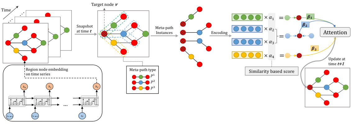
The overall architecture of the proposed STMEC model is shown in Figure 2. Different from existing graph based crime prediction models which represent the links between regions by either geographical distance or similarity of points of interest (POI), we model the interaction between regions via an intermediate node of a certain attribute type (e.g., demographic distribution). These interactions are characterized as symmetric meta-paths such as $\langle region,factor,region\rangle$ on a meta-path based graph. Given the temporal properties of this meta-path based graph, the embedding of each region is learned and updated along the time steps. To achieve better representation learning for regions, the procedure is decomposed into four steps. Firstly, the initial embedding of each region is obtained by learning the latent representations of local crime trends with a recurrent neural network (i.e., Long Short-Term Memory networks (LSTM)). Secondly, for each meta-path instance, we integrate the embeddings of attributes and regions along the path. Thirdly, similarity based weights are computed and assigned to meta-path instances to improve the interpretability and accuracy of the model. In this step, the weights are conditioned on the attribute distributions between the pair of regions, and we obtain the representation via weighted aggregation of all meta-path instances of the same type. Finally, the final representation of aggregated meta-paths is generated via an attention mechanism to facilitate predictions. The attention weights help reason out the contributions of different attribute types, providing insights into crime prevention.

We firstly learn the latent representation of each region at every time step from the criminal records. For sequential data modeling, LSTM is known for its ability to capture both short-term and long-term dependencies when compared with other RNN based models Felix01. Thus, in this task, we deploy a time-series oriented LSTM to learn latent representations from the given sequence of crime records.

For each region $r_{i}$, given a list of crime records containing $T$ daily data points $\mathcal{Y}_{i}=\{\mathbf{y}_{i}^{1},\mathbf{y}_{i}^{2},\ldots,\mathbf{y}_{i}^{t},\ldots\mathbf{y}_{i}^{T}\}\in\mathbb{R}^{T\times C}$, where $\mathbf{y}_{i}^{t}\in\mathbb{R}^{C}$ is the number of crime records for all crime types $C$ at time step $t$. We aim to initialize the representation of region $r_{i}$ at time step $t$ based on the crime records from previous $M$ time steps, which is denoted as $\mathcal{Y}_{i}^{M}=\{\mathbf{y}_{i}^{t-M+1},\ldots,\mathbf{y}_{i}^{t}\}\in\mathbb{R}^{M\times C}$. By taking a region’s features $\mathbf{y}$ at different time steps as the input, the hidden states $\mathbf{h}_{r_{i}}^{t}$ derived from the LSTM will be utilized as the initial representation of region $r_{i}$ at time step $t$. An LSTM unit is composed of a forget gate, an input gate, and an output gate, which regulate the flow of information. Formally, the LSTM layer performs the following functions to update the hidden states $\mathbf{h}_{r_{i}}^{t}$:

where $\mathbf{y}_{i}^{t}$ is the input at time $t$ with dimension $d_{y}$, and $\mathbf{h}_{r_{i}}^{t}$ is the hidden state at time $t$ with dimension $d_{s}$. Furthermore, the input gate, forget gate, output gate and cell state are denoted as $\mathbf{i}_{r_{i}}^{t}$, $\mathbf{f}_{r_{i}}^{t}$, $\mathbf{o}_{r_{i}}^{t}$, and $\mathbf{c}_{r_{i}}^{t}$, respectively. Each of the $\mathbf{W}_{x*}\in\mathbb{R}^{{d_{y}}\times{d_{s}}}$ is the weight matrix to control information flow from input to LSTM cell, while each of the $\mathbf{W}_{h*}\in\mathbb{R}^{{d_{s}}\times{d_{s}}}$ is the weight matrix to transform the previous states $\mathbf{h}_{r_{i}}^{t-1}$ to LSTM cell. Also, $\mathbf{b}_{*}\in\mathbb{R}^{d_{s}}$ represents the bias term. The sigmoid function denoted as $\sigma$ helps the LSTM cell to update or forget the data. For notation simplicity, we denote Eq. 1 as $\mathbf{h}_{r_{i}}^{t}=\mathrm{LSTM}(*,\mathbf{c}_{r_{i}}^{t-1},\mathbf{h}_{r_{i}}^{t-1})$ in the following subsections.

In crime prediction tasks, external features depicting the community profiles are normally considered as auxiliary knowledge to complement the machine learning methods. For instance, demographics, income level, and human behavioral factors indicating the socioeconomic characteristics 10.1145/2663204.2663254; Fateha01 are commonly used to improve the crime incident prediction. However, how to leverage heterogeneous and ubiquitous information effectively is always a challenge. In this case, the meta-path based graph is considered to represent heterogeneous information as it can model various relationships between different types of objects intuitively and precisely. Different meta-path based embedding techniques, such as the random-walk based methods 10.1145/3097983.3098036; 10.1109/TKDE.2018.2833443 (i.e., Metapath2vec and HERec), are proposed to aggregate information from neighbors along the paths but are generally more focused on the structural information of each meta-path type and simply treat the inherent node attributes as features. However, in the crime prediction context, how the regions correlate and interact with those features are crucial to accurate predictions. In general, criminal activities always interact with different socioeconomic factors, and the relations can be modeled in a symmetric structure denoted as $\langle region,factor,region\rangle$. This structure protects the diversity of auxiliary information and maps the correlation between regions in terms of different views. Thus, inspired by 10.1145/3366423.3380297, we distill comprehensive semantics by differentiating meta-path instances into different categories and integrating information by meta-path aggregation methods. In this work, we consider six factors as potential causes of crime-prone communities, including demographics, income level, job type, journey to work, urban facilities, and geographical distance. Each factor is represented by a vector that describes the distribution of its attributes. For example, a feature vector for urban facilities carries the proportion of recreation, residential, and public safety facilities.

It is also worth mentioning that, we consider only symmetric meta-paths for capturing region-wise similarity. For example, if two regions have similar income statistics, they will be connected by a virtual meta-path link as $\langle region,income,region\rangle$ (RIR), and it can be extended to RIRIR which has a length of more than 2, but it will reduce the training efficiency as more steps of aggregation are involved. Also, as we focus on learning the importance of different factors to the prediction results, asymmetric meta-path like $\langle region,income,region,job,region\rangle$ (RIRJR) is likely to introduce more noise in the meta-path instance, and will bring difficulties in quantifying the contributions of different socioeconomic factors like income and job in this case. Furthermore, asymmetric meta-paths come with a higher demand on the feature engineering process that heavily depends on domain expertise.

Given target region $r_{i}$ for which we want to predict the crime incidents in the next time step $t+1$, we first take the snapshot of the entire meta-path based graph at time $t$. In the snapshot, we can find a candidate region $r_{j}$ connects to $r_{i}$ via an intermediate node indicating a certain factor. As a meta-path is defined by $\langle region,factor,region\rangle$, we denote the meta-path instance as $p(r_{i},r_{j})$ and the intermediate node as $m^{p(r_{i},r_{j})}$, where the type of meta-path instance $P_{A}$ is determined by the type of intermediate node $A\in\mathcal{A}$. For each type of meta-path, the basic idea is to find all meta-path instances containing target node $r_{i}$ and measure the priority of each instance. This is achieved by quantifying the similarity between the target region and another region w.r.t. their relationships towards the intermediate node. For instance, if region $r_{i}$ and region $r_{j}$ both belong to low-income areas, they will be connected by the intermediate node $income$. If $r_{j}$ has similar measurements regarding the income-related features (i.e., mean, median, and variance in our case), we would consider $r_{j}$ as an important candidate for predicting events that happen in $r_{i}$ when modeling the $\langle region,income,region\rangle$ meta-path. Section 3.4 further introduces the computation of pairwise similarities between two regions in a meta-path instance.

We denote region $r_{i}$’s feature vector of a certain factor as $\mathbf{m}_{r_{i}}$. For example, the feature vector that describes the region’s income level comprises of the median, mean, variance, and stand deviation of the local income. To embed the information along a particular path instance into a low-dimensional vector, we concatenate the node features to preserve the heterogeneity yili01; 8731426. Following the concatenation, we apply a linear transformation to map the sequence of features into the same latent space. For a meta-path instance $p(r_{i},r_{j})$, we denote its embedding at time $t$ as follows:

where $\mathbf{h}_{p(r_{i},r_{j})}\in\mathbb{R}^{d_{e}}$ is the meta-path instance embedding, and $\mathbf{W}_{p}\in\mathbb{R}^{d_{e}\times d^{\prime}}$ is the learnable parameter. Here, $d^{\prime}$ is the dimension of the concatenated feature vector and $d_{e}$ is the embedding size of the concatenated features. In addition, $\mathbf{h}_{r_{i}}^{t}$ is the temporal embedding of region $r_{i}$ learnt from the previous $M$ time steps.

To aggregate information from meta-path instances for target node $r_{i}$, we can perform a weighted sum of the instances for each type of meta-path $P_{A}$:

where $r_{*}$ denotes the candidate region connected by a meta-path instance belonging to type $P_{A}$ and ends at region $r_{i}$. The similarity score $s(r_{i},r_{*})$ is computed by our proposed distribution-aware PathSim. In what follows, we present the innovative design of this path based similarity metric.

PathSim 10.14778/3402707.3402736 is a well-established method that outstands for its ability to capture the subtle semantic similarities between objects in symmetric meta-paths. The original PathSim is presented below:

However, the original PathSim relies only on occurrences of categorical node features and lacks an effective approach to take into account the fine-grained, sub-divided categorical features when computing two regions’ similarity in the crime prediction context. For example, in the meta-path with $urban\,facilities$ as the intermediate node, a vector containing proportions of different building facilities has been used to indicate the urbanization level of a region. A building facility is described as a commonplace that accommodates diverse activities, such as residential, civic, educational, or commercial facilities. These types of facilities are further subdivided into more specific facility types like high school and primary school in the category of educational facilities. Such sub-divided categorical features are commonly observed within the ubiquitous data, making the traditional PathSim incompatible. This is because the similarity between regions w.r.t. different fine-grained categorical features are treated evenly in PathSim, which leads to significant information loss. Hence, we propose a distribution-aware PathSim to complement the similarity metrics. The distribution-aware PathSim $s(r_{i},r_{j})$ for two regions is given by:

where $z$ represents the facility category (e.g., $Educational$), $Z$ indicates all types of urban facilities, and $\mathcal{P}_{z}$ denotes the meta-path connected by the category $z$. Here, $\lvert z\rvert$ and $\lvert Z\rvert$ denote the number of facility types in category $z$ and the number of facility types across all categories. For example, region $r_{1}$ in Table 2 has two categories of urban facilities as $Educational$ and $Recreational$, where $Elementary\ School$ and $High\ School$ are the 2 facility types of $Educational$, and there are in total 4 facility types: $Elementary\ School$, $High\ School$, $Zoo$, and $Pool$ across all categories. Thus, $\frac{\lvert z\rvert}{\lvert Z\rvert}$ can represent the proportion of $Educational$ in all facility types as $\frac{2}{4}$. Also, $s\left(r_{i},z,r_{j}\right)$ represents the similarity score between region $r_{i}$ and $r_{j}$ in terms of the category $z$, while $s\left(r_{i},r_{j}\right)$ is the similarity between two regions concerning all categories $Z$. The measurement is mainly based on the number of path instances between two regions, which is denoted as $\lvert p_{r_{i}\rightarrow r_{j}}\rvert$.

To demonstrate how our proposed method works, we use a toy example as shown in Table 2 to illustrate the reliability of the method compared with the original PathSim. The example shows the number of urban facilities in region $r_{1}$, $r_{2}$, and $r_{3}$. The urban facilities can be divided into two categories as $Educational$ and $Recreational$, and each has two facility types as $Elementary\ School$ and $High\ School$, $Zoo$ and $Pool$ respectively. We aim to find the region with the most similar structure as $r_{1}$. As $r_{2}$ has both educational and recreational facilities of the same amount, it is more close to the urban structure as $r_{1}$. PathSim measures the similarity scroes as: $s^{\prime}(r_{1},r_{2})=\frac{2\times\left(2\times 2+2\times 2+5\times 10\right)}{\left(2\times 2+2\times 2+5\times 5+5\times 5\right)+\left(2\times 2+2\times 2+10\times 10\right)}=0.699$, while $s^{\prime}(r_{1},r_{3})=0.926$. The distribution-aware PathSim complements the problem by taking the weighted sum of PathSim in terms of categories. Thus, we compute the similarity score as $s(r_{1},r_{2})=\frac{2}{4}\cdot 1+\frac{2}{4}\cdot\frac{2\times\left(5\times 10\right)}{\left(5\times 5+5\times 5\right)+\left(10\times 10\right)}=0.833$, while $s(r_{1},r_{3})=0.5$. Apparently, our distribution-aware PathSim has stronger consistency with human intuition owing to the consideration of different categories.

Intuitively, different meta-paths carry different semantics in a region-region interaction. In the task of crime prediction, it is hard to identify the leading factor that contributes more to criminal behaviors. Also, for different regions, a meta-path may have varying semantics as it collects information from different instances via the interaction. Hence, we apply a graph attention layer to rank the importance of meta-paths and then summarize the flow of information by weighted sum.

For region $r_{i}\in I$, we have the summarization of the meta-path $P_{A}$ denoted as $\mathbf{h}_{r_{i}}^{P_{A}}$, where $P_{A}\in\mathcal{P}$ and $\mathcal{P}$ is a set of meta-paths containing node $r_{i}$. First, we transform the meta-path based representations for all nodes $r_{i}\in I$, and obtain the average value with respect to each meta-path type $P_{A}$:

where $\mathbf{M}_{u}\in\mathbb{R}^{d_{a}\times d_{e}}$ and $\mathbf{b}_{u}\in\mathbb{R}^{d_{a}}$ are learnable parameters. The number of nodes is denoted by $|I|$.

Then the attention mechanism is utilized to fuse the meta-path based context, the weights are learnt over different types of meta-path as follows:

where $\mathbf{q}\in\mathbb{R}^{d_{a}}$ is the attention vector to be learned in the training process, and $\beta^{P_{A}}$ is the learnt importance score of meta-path $P_{A}$. The summarized context information based on each type of meta-path is embedded as $\mathbf{h}_{r_{i}}^{\mathcal{P}}$, which will be projected to a $C$-dimensional output via a dense layer with sigmoid activation. The final output is the estimated probability of crime $c$ that will happen in region $r_{i}$, which is denoted as $\hat{y}_{r_{i}}^{t,c}$.

Our objective is to obtain the value of $\hat{\mathbf{y}}_{r_{i}}^{t}$ at each time step $t$, where the $c$-th element $\hat{y}_{r_{i}}^{t,c}$ denotes the probability that crime event of category $c$ will happen in the next time step $t+1$. As this can be viewed as $C$ binary classification tasks, we employ cross entropy as the loss function:

where $\hat{y}_{r_{i}}^{t,c}$ is the estimated probability of crime $c$ that will happen in region $r_{i}$ in the next time slot $t+1$ and $y_{r_{i}}^{t+1,c}$ is the corresponding ground-truth record at time slot $t+1$. Also, $S$ is the crime event set in the training process. In this work, the model parameters are learnt by minimizing the loss function with Adaptive Moment Estimation (Adam) Diederik01.

In our work, the hyperparameters of each baseline model are carefully tuned to ensure optimal results. We implement STMEC with Pytorch architecture. We set the dimension of temporal embedding $d_{s}$ as $128$ and the number of LSTM layers as $2$. The optimal time window $M$, from which the temporal dynamics are learned, is set as $28$ days for 2015 dataset and $21$ days for 2014 dataset. Also, The embedding size of meta-path instances $d_{e}$ is set as $64$ and the attention vector size $d_{a}$ is set as $128$. Additionally, the learning process is optimized by Adam, with the learning rate 0.0001. The effect of different hyperparameter setting has been discussed in Section 4.5.

We investigate 6 different types of factors that may affect the criminal activities which are represented as meta-paths: $\langle region,demographic,region\rangle$ (RDR), $\langle region,income,region\rangle$ (RIR), $\langle region,job\>type,region\rangle$ (RJR), $\langle region,commuting\>ways,region\rangle$ (RCR), $\langle region,urbanization,region\rangle$ (RUR), and $\langle region,geographic,region\rangle$ (RGR). The importance of the factors is discussed in the following subsections.

Apart from the superior performance given by STMEC, another contribution of the framework is to give explanations on forecasts. This work involves 6 different types of meta-paths which represent the features from different categories of potential factors. As we generate pre-defined region-to-region instances and sum up the impacts from each path by a given similarity score, the effect of the black box is relieved by explicitly modeling the interactions and ranking priorities of the path instances. Furthermore, the attention mechanism that obtains the weight of each meta-path type also helps to rank the importance of factors in the crime prediction tasks. Table 6 demonstrates the summary of importance sores with respect to different factors. As the scores are obtained from each test instance given by day, the result indicates that the importance of each factor varies a lot along the timeline. Specifically, we can observe the variation of importance for each factor from Figure 8. It shows that urbanization level is the leading factor for most of our predictions, while the type of job in the population is the least important factor in the task. Additionally, we can also observe that the impact of geographical information is relatively stable, while the others dramatically change up and down. It is worth noticing that the causes of criminal activities are not constant along the time. This observation supports our idea of constructing the model by considering the variations and interactions between features.

To understand the significance of different components in our proposed framework, we further examine the efficacy of the attention module and the distribution-aware PathSim by replacing them with a mean aggregator in the degraded variants of STMEC. In general, the experimental results in Figure 11 have shown that both key components are beneficial to the performance of our model. Besides, attention module reflects more significance on predicting crimes of NYC 2014, while PathSim shows more potential in predicting crimes of NYC 2015.

This work has been reviewed by the Research Ethics and Integrity and is deemed to be exempt from ethics review under the National Statement on Ethical Conduct in Human Research and relevant University of Queensland policy (PPL 4.20.07).

This article does not contain any experimentation with human or animal subjects.

Not applicable.

All datasets used for supporting the conclusions of this article are available from the public data repository at the website of data.cityofnewyork.us and www.kaggle.com.

All authors have no competing interests as defined by Springer, or other interests that might be perceived to influence the results and/or discussion reported in this paper.

No funding was received for conducting this study.

Yuting Sun implemented the methodology, performed data curation, wrote the original draft, and conducted the experiment.

Tong Chen proposed the conceptualization and methodology, prepared the figures, and performed review and editing.

Hongzhi Yin proposed the research problem and methodology, supervised the whole research work, wrote the introduction and abstract parts, and performed review and editing.

We gratefully thank Dr. Thomas Taimre (the University of Queensland) and Dr. Radislav Vaisman (the University of Queensland) for valuable discussions on this research and helpful comments on the manuscript. This work is supported by Australian Research Council Future Fellowship (Grant No. FT210100624) and Discovery Project (Grant No.DP190101985).

Yuting Sun, Ph.d candidature, School of Information Technology and Electrical Engineering, the University of Queesnland, Brisbane, Australia.

Tong Chen, Lecturer, School of Information Technology and Electrical Engineering, the University of Queesnland, Brisbane, Australia.

Hongzhi Yin, Associate Professor/ARC Future Fellow, School of Information Technology and Electrical Engineering, the University of Queesnland, Brisbane, Australia.

References

- (1) GBD 2017 Causes of Death Collaborators: Global, regional, and national age-sex-specific mortality for 282 causes of death in 195 countries and territories, 1980–2017: a systematic analysis for the global burden of disease study 2017. The Lancet 392(10159), 1736–1788 (2018). https://doi.org/10.1016/S0140-6736(18)32203-7
- (2) Russell, S.: Estimating the costs of serious and organised crime in australia 2016–17. Statistical Report 9, Australian Institute of Criminology, Canberra (October 2018)
- (3) de Melo, S.N., Pereira, D.V.S., Andresen, M.A.: Spatial-temporal variations of crime: A routine activity theory perspective. International Journal of Offender Therapy and Comparative Criminology 62(7), 1967–1991 (2017). https://doi.org/10.1177/0306624X17703654
- (4) Li, Z., Zhang, T., Yuan, Z., Wu, Z., Du, Z.: Spatio-temporal pattern analysis and prediction for urban crime. In: 2018 Sixth International Conference on Advanced Cloud and Big Data (CBD), pp. 177–182 (2018). https://doi.org/10.1109/CBD.2018.00040
- (5) Nafi’iyah, N., Mauladi, K.F.: Linear regression analysis and svr in predicting motor vehicle theft. In: 2021 International Seminar on Application for Technology of Information and Communication (iSemantic), pp. 54–58 (2021). https://doi.org/10.1109/iSemantic52711.2021.9573225
- (6) Zhao, X., Tang, J.: Modeling temporal-spatial correlations for crime prediction. In: Proceedings of the 2017 ACM on Conference on Information and Knowledge Management. CIKM ’17, pp. 497–506 (2017). https://doi.org/10.1145/3132847.3133024
- (7) Yi, F., Yu, Z., Zhuang, F., Zhang, X., Xiong, H.: An integrated model for crime prediction using temporal and spatial factors. In: 2018 IEEE International Conference on Data Mining (ICDM), pp. 1386–1391 (2018). https://doi.org/10.1109/ICDM.2018.00190
- (8) Huang, C., Zhang, J., Zheng, Y., Chawla, N.V.: Deepcrime: Attentive hierarchical recurrent networks for crime prediction. In: Proceedings of the 27th ACM International Conference on Information and Knowledge Management. CIKM ’18, pp. 1423–1432 (2018). https://doi.org/10.1145/3269206.3271793
- (9) Huang, C., Zhang, C., Zhao, J., Wu, X., Yin, D., Chawla, N.: Mist: A multiview and multimodal spatial-temporal learning framework for citywide abnormal event forecasting. In: The World Wide Web Conference. WWW ’19, pp. 717–728 (2019). https://doi.org/10.1145/3308558.3313730
- (10) Snaphaan, T., Hardyns, W.: Environmental criminology in the big data era. European Journal of Criminology 18(5), 713–734 (2021). https://doi.org/10.1177/1477370819877753
- (11) Chen, H., Yin, H., Sun, X., Chen, T., Gabrys, B., Musial, K.: Multi-level graph convolutional networks for cross-platform anchor link prediction. In: Proceedings of the 26th ACM SIGKDD International Conference on Knowledge Discovery & Data Mining. KDD ’20, pp. 1503–1511 (2020). https://doi.org/10.1145/3394486.3403201
- (12) Wang, Y., Ge, L., Li, S., Chang, F.: Deep temporal multi-graph convolutional network for crime prediction. In: Conceptual Modeling - 39th International Conference. ER 2020, pp. 525–538 (2020). https://doi.org/10.1007/978-3-030-62522-1_39
- (13) Lin, Y., Yen, M., Yu, L.: Grid-based crime prediction using geographical features. ISPRS International Journal of Geo-Information 7(8:298) (2018). https://doi.org/10.3390/ijgi7080298
- (14) Weatherburn, D.: What causes crime. Crime and Justice Bulletin (2001)
- (15) Glaeser, E.L., Sacerdote, B.: Why is there more crime in cities? Journal of Political Economy 107(S6), 225–258 (1999). https://doi.org/10.1086/250109
- (16) Bappee, F.K., Petry, L.M., Soares, A., Matwin, S.: Analyzing the impact of foursquare and streetlight data with human demographics on future crime prediction. In: Advances in Data Science and Information Engineering. ICMI ’14, pp. 435–449 (2021). https://doi.org/10.1007/978-3-030-71704-9_29
- (17) Almanie, T., Mirza, R., Lor, E.: Crime prediction based on crime types and using spatial and temporal criminal hotspots. International Journal of Data Mining & Knowledge Management Process (IJDKP) 5(4) (2015). https://doi.org/10.5121/ijdkp.2015.5401
- (18) Alves, L.G.A., Ribeiro, H.V., Rodrigues, F.A.: Crime prediction through urban metrics and statistical learning. Physica A: Statistical Mechanics and its Applications 505, 435–443 (2018). https://doi.org/10.1016/j.physa.2018.03.084
- (19) Saltos, G., Coceas, M.: An exploration of crime prediction using data mining on open data. International Journal of Information Technology & Decision Making 16(5), 1155–1181 (2017). https://doi.org/10.1142/S0219622017500250
- (20) Sun, Y., Han, J., Yan, X., Yu, P.S., Wu, T.: Pathsim: Meta path-based top-k similarity search in heterogeneous information networks. Proceedings of the VLDB Endowment 4(11), 992–1003 (2011). https://doi.org/10.14778/3402707.3402736
- (21) Hussein, R., Yang, D., Cudré-Mauroux, P.: Are meta-paths necessary? revisiting heterogeneous graph embeddings. In: Proceedings of the 27th ACM International Conference on Information and Knowledge Management (CIKM), pp. 437–446 (2018). https://doi.org/10.1145/3269206.3271777
- (22) Chen, T., Yin, H., Ren, J., Huang, Z., Zhang, X., Wang, H.: Uniting heterogeneity, inductiveness, and efficiency for graph representation learning. IEEE Transactions on Knowledge and Data Engineering (2021). https://doi.org/10.1109/TKDE.2021.3100529
- (23) Wang, B., Lin, Y., Guo, S., Wan, H.: Gsnet: Learning spatial-temporal correlations from geographical and semantic aspects for traffic accident risk forecasting. In: Proceedings of the AAAI Conference on Artificial Intelligence, vol. 35, pp. 4402–4409 (2021)
- (24) Gers, F.A., Eck, D., Schmidhuber, J.: Applying lstm to time series predictable through time-window approaches. In: Proceedings of the 12th Italian Workshop on Neural Nets. Neural Nets WIRN Vietri-01, pp. 193–200 (2002). https://doi.org/10.1007/978-1-4471-0219-9_20
- (25) Bogomolov, A., Lepri, B., Staiano, J., Oliver, N., Pianesi, F., Pentland, A.: Once upon a crime: Towards crime prediction from demographics and mobile data. In: Proceedings of the 16th International Conference on Multimodal Interactions. ICMI ’14, pp. 427–434 (2014). https://doi.org/10.1145/2663204.2663254
- (26) Dong, Y., Chawla, N.V., Swami, A.: Metapath2vec: Scalable representation learning for heterogeneous networks. In: Proceedings of the 23rd ACM SIGKDD International Conference on Knowledge Discovery and Data Mining. KDD ’17, pp. 135–144 (2017). https://doi.org/10.1145/3097983.3098036
- (27) Shi, C., Hu, B., Zhao, W.X., Yu, P.S.: Heterogeneous information network embedding for recommendation. IEEE Trans. on Knowl. and Data Eng. 31(2), 357–370 (2019). https://doi.org/10.1109/TKDE.2018.2833443
- (28) Fu, X., Zhang, J., Meng, Z., King, I.: Magnn: Metapath aggregated graph neural network for heterogeneous graph embedding. In: Proceedings of The Web Conference 2020. WWW ’20, pp. 2331–2341 (2020). https://doi.org/10.1145/3366423.3380297
- (29) Li, Y., Jin, Y., Song, G., Zhu, Z., Shi, C., Wang, Y.: Graphmse: Efficient meta-path selection in semantically aligned feature space for graph neural networks. In: Proceedings of the AAAI Conference on Artificial Intelligence 2021. AAAI ’21, pp. 4206–4214 (2021)
- (30) Chen, H., Yin, H., Chen, T., Nguyen, Q.V.H., Peng, W.-C., Li, X.: Exploiting centrality information with graph convolutions for network representation learning. In: 2019 IEEE 35th International Conference on Data Engineering (ICDE), pp. 590–601 (2019). https://doi.org/10.1109/ICDE.2019.00059
- (31) Kingma, D.P., Ba, J.: Adam: A method for stochastic optimization. In: The 3rd International Conference for Learning Representations. ICLR ’15 (2015)
- (32) MuonNeutrino: Demographic, economic, and location data for census tracts in nyc. Kaggle (2017)
- (33) Department of Information Technology and Telecommunications (DOITT): Points of interest. NYC Open Data (2016)
- (34) Police Department (NYPD): Nypd complaint data historic. NYC Open Data (2016)
- (35) Green, B., Horel, T., Papachristos, A.V.: Modeling contagion through social networks to explain and predict gunshot violence in chicago, 2006 to 2014. JAMA Internal Medicine 177(3), 326–333 (2017). https://doi.org/10.1001/jamainternmed.2016.8245
- (36) Huang, C., Wu, X., Zhang, X., Zhang, C., Zhao, J., Yin, D., Chawla, N.V.: Online purchase prediction via multi-scale modeling of behavior dynamics. In: Proceedings of the 25th ACM SIGKDD International Conference on Knowledge Discovery & Data Mining. KDD ’19, pp. 2613–2622 (2019). https://doi.org/10.1145/3292500.3330790
- (37) Munnelly, G., Lawless, S.: Investigating entity linking in early english legal documents. In: Proceedings of the 18th ACM/IEEE on Joint Conference on Digital Libraries. JCDL ’18, pp. 59–68 (2018). https://doi.org/10.1145/3197026.3197055
- (38) Jin, G., Wang, Q., Zhu, C., Feng, Y., Huang, J., Zhou, J.: Addressing crime situation forecasting task with temporal graph convolutional neural network approach. In: 2020 12th International Conference on Measuring Technology and Mechatronics Automation (ICMTMA). KDD ’19, pp. 474–478 (2020). https://doi.org/10.1109/ICMTMA50254.2020.00108
- (39) Han, X., Hu, X., Wu, H., Shen, B., Wu, J.: Risk prediction of theft crimes in urban communities: An integrated model of lstm and st-gcn. IEEE Access 8, 217222–217230 (2020). https://doi.org/10.1109/ACCESS.2020.3041924
- (40) Liang, W., Wang, Y., Tao, H., Cao, J.: Towards hour-level crime prediction: A neural attentive framework with spatial–temporal-categorical fusion. Neurocomputing (2021). https://doi.org/10.1016/j.neucom.2021.11.052
- (41) Kipf, T.N., Welling, M.: Semi-supervised classification with graph convolutional networks. In: The 5th International Conference on Learning Representations. ICLR 2017 (2017)
- (42) Zhao, L., Song, Y., Zhang, C., Liu, Y., Wang, P., Lin, T., Deng, M., Li, H.: T-gcn: A temporal graph convolutional network for traffic prediction. IEEE Transactions on Intelligent Transportation Systems 21(9), 3848–3858 (2020). https://doi.org/10.1109/TITS.2019.2935152
- (43) Deng, S., Rangwala, H., Ning, Y.: Learning dynamic context graphs for predicting social events. In: Proceedings of the 25th ACM SIGKDD International Conference on Knowledge Discovery & Data Mining. KDD ’19, pp. 1007–1016 (2019). https://doi.org/10.1145/3292500.3330919
- (44) Yu, B., Yin, H., Zhu, Z.: Spatio-temporal graph convolutional networks: A deep learning framework for traffic forecasting. In: Proceedings of the Twenty-Seventh International Joint Conference on Artificial Intelligence. IJCAI-18, pp. 3634–3640 (2018). https://doi.org/10.5555/3304222.3304273
- (45) Wang, C., Lin, Z., Yang, X., Sun, J., Yue, M., Shahabi, C.: Hagen: Homophily-aware graph convolutional recurrent network for crime forecasting. In: Proceedings of the AAAI Conference on Artificial Intelligence, pp. 4193–4200 (2022)
- (46) Song, G., Bernasco, W., Liu, L., Xiao, L., Zhou, S., Liao, W.: Crime feeds on legal activities: Daily mobility flows help to explain thieves’ target location choices. Journal of Quantitative Criminology 35(26), 831–854 (2019). https://doi.org/10.1007/s10940-019-09406-z
- (47) Rumi, S.K., Deng, K., Salim, F.D.: Theft prediction with individual risk factor of visitors. In: Proceedings of the 26th ACM SIGSPATIAL International Conference on Advances in Geographic Information Systems. SIGSPATIAL ’18, pp. 552–555 (2018). https://doi.org/10.1145/3274895.3274994
- (48) Rumi, S.K., Salim, F.D.: Modelling regional crime risk using directed graph of check-ins. In: Proceedings of the 29th ACM International Conference on Information & Knowledge Management. CIKM ’20, pp. 2201–2204 (2020). https://doi.org/10.1145/3340531.3412065
- (49) Kadar, C., Pletikosa, I.: Mining large-scale human mobility data for long-term crime prediction. EPJ Data Science 7(26) (2018). https://doi.org/10.1140/epjds/s13688-018-0150-z
- (50) Rosés, R., Kadar, C., Malleson, N.: A data-driven agent-based simulation to predict crime patterns in an urban environment. Computers, Environment and Urban Systems 89(101660) (2021). https://doi.org/10.1016/j.compenvurbsys.2021.101660
- (51) Wang, Z., Jiang, R., Cai, Z., Fan, Z., Liu, X., Kim, K.-S., Song, X., Shibasaki, R.: Spatio-temporal-categorical graph neural networks for fine-grained multi-incident co-prediction. In: Proceedings of the 30th ACM International Conference on Information & Knowledge Management. CIKM ’21, pp. 2060–2069 (2021). https://doi.org/10.1145/3459637.3482482
- (52) Park, S., Serrà, J., Martinez, E.F., Oliver, N.: Mobinsight: A framework using semantic neighborhood features for localized interpretations of urban mobility. ACM Transactions on Interactive Intelligent Systems 8(3) (2018). https://doi.org/10.1145/3158433
- (53) Fengli Xu, Z.L., Xia, T., Guo, D., Li, Y.: Sume: Semantic-enhanced urban mobility network embedding for user demographic inference. Proceedings of the ACM on Interactive, Mobile, Wearable and Ubiquitous Technologies 4(3), 1–25 (2020). https://doi.org/10.1145/3411807
- (54) Yang, D., Qu, B., Yang, J., Cudré-Mauroux, P.: Lbsn2vec++: Heterogeneous hypergraph embedding for location-based social networks. IEEE Transactions on Knowledge and Data Engineering 34, 1843–1855 (2020). https://doi.org/10.1109/TKDE.2020.2997869
- (55) Huang, Y., Bi, H., Li, Z., Mao, T., Wang, Z.: Stgat: Modeling spatial-temporal interactions for human trajectory prediction. In: Proceedings of the IEEE/CVF International Conference on Computer Vision. ICCV ’19, pp. 6272–6281 (2019). https://doi.org/10.1109/ICCV.2019.00637
- (56) Wang, S., Miao, H., Chen, H., Huang, Z.: Multi-task adversarial spatial-temporal networks for crowd flow prediction. In: Proceedings of the 29th ACM International Conference on Information & Knowledge Management. CIKM ’20, pp. 1555–1564 (2020). https://doi.org/10.1145/3340531.3412054
- (57) Chen, T., Yin, H., Chen, H., Wu, L., Wang, H., Zhou, X., Li, X.: Tada: trend alignment with dual-attention multi-task recurrent neural networks for sales prediction. In: 2018 IEEE International Conference on Data Mining (ICDM), pp. 49–58 (2018). IEEE
- (58) Chen, T., Yin, H., Nguyen, Q.V.H., Peng, W.-C., Li, X., Zhou, X.: Sequence-aware factorization machines for temporal predictive analytics. In: 2020 IEEE 36th International Conference on Data Engineering (ICDE), pp. 1405–1416 (2020). IEEE
- (59) Tam, N.T., Weidlich, M., Zheng, B., Yin, H., Hung, N.Q.V., Stantic, B.: From anomaly detection to rumour detection using data streams of social platforms. Proceedings of the VLDB Endowment 12(9), 1016–1029 (2019)
- (60) Trung, H.T., Van Vinh, T., Tam, N.T., Yin, H., Weidlich, M., Hung, N.Q.V.: Adaptive network alignment with unsupervised and multi-order convolutional networks. In: 2020 IEEE 36th International Conference on Data Engineering (ICDE), pp. 85–96 (2020). IEEE
- (61) Yao, H., Liu, Y., Wei, Y., Tang, X., Li, Z.: Learning from multiple cities: A meta-learning approach for spatial-temporal prediction. In: The World Wide Web Conference. WWW ’19, pp. 2181–2191 (2019). https://doi.org/10.1145/3308558.3313577
- (62) Wang, H., Kifer, D., Graif, C., Li, Z.: Crime rate inference with big data. In: Proceedings of the 22nd ACM SIGKDD International Conference on Knowledge Discovery and Data Mining, pp. 635–644 (2016). https://doi.org/10.1145/2939672.2939736
- (63) Wang, T., Rudin, C., Wagner, D., Sevieri, R.: Learning to detect patterns of crime. In: Joint European Conference on Machine Learning and Knowledge Discovery in Databases (ECML), pp. 515–530 (2013). https://doi.org/10.1007/978-3-642-40994-3_33
- (64) Yang, D., Heaney, T., Tonon, A., Wang, L., Cudré-Mauroux, P.: Crimetelescope: crime hotspot prediction based on urban and social media data fusion. World Wide Web 21(5), 1323–1347 (2018). https://doi.org/10.1007/s11280-017-0515-4
- (65) Zhao, X., Fan, W., Liu, H., Tang, J.: Multi-type urban crime prediction. In: Proceedings of the AAAI Conference on Artificial Intelligence (2022)