Holographic Schwinger effect and electric instability with anisotropy
Abstract
According to the gauge-gravity duality, we systematically study the Schwinger effect and electric instability with anisotropy in a top-down holographic approach. The anisotropic black brane and bubble (soliton) background in IIB supergravity are employed and the dual theories in these backgrounds are expected to be anisotropic theory at finite temperature and anisotropic theory with confinement respectively. Then performing the potential analysis, we find due to the anisotropy, the potential barrier behaves oppositely with parallel and perpendicular electric fields, and this behavior agrees with the previous study about the quark potential with anisotropy in this system. Afterwards, we evaluate the pair production rate by solving the equation of motion for a fundamental string numerically which reveals the consistent behavior with the potential analysis. Furthermore, the probe D7-brane as flavor is introduced into the bulk in order to investigate the electric instability. The vacuum decay rate can be obtained by evaluating the imaginary part of the D7-brane action which again agrees with our potential analysis. Solving the associated constraint of gauge field strength on the flavor brane, we finally obtain the V-A curve displaying the distinct behavior of the conductivity in parallel and perpendicular direction which is in agreement with some bottom-up and phenomenologically holographic approaches in anisotropic fluid. Accordingly, we believe this work may be remarkable to study the electric features in strongly coupled anisotropic system.
Si-wen Li11 1 Email: siwenli@dlmu.edu.cn, Sen-kai Luo22 2 Email: luosenkai@dlmu.edu.cn, Hao-qian Li33 3 Email: lihaoqian@dlmu.edu.cn,
Department of Physics, School of Science,
Dalian Maritime University,
Dalian 116026, China
1 Introduction
There are many interesting phenomena in the heavy-ion collision experiment, especially under the strong electromagnetic field created by the collision of the charged particles. The Schwinger effect is one of the most significant phenomenon in the heavy-ion collision since it relates to the particle production rate. Specifically, due to the high speed of the charged particles, an extremely strong electromagnetic field would be generated in the collision so that virtual pairs of particles in the vacuum are able to be excited by the electromagnetic field to become real particles [1, 2]. In this sense, the Schwinger effect may be remarkable to understand the process of particle creation and thermalization in the heavy-ion collision. On the other hand, many researches reveal that the product in the heavy-ion collision, i.e. the quark-gluon plasma (QGP), is strongly coupled [3, 4] with anisotropic pressure [5, 6, 7, 8]. So when the collision occurs, it forms highly dense and anisotropic situation with extremely strong electromagnetic field, therefore the Schwinger effect would appear and be affected by the anisotropy. In this sense, investigating the Schwinger effect in an anisotropic dense situation would be very constructive to the experiment of heavy-ion collision.
However the calculations in [1, 2] imply Schwinger effect is non-perturbative, thus it is very challenging to evaluate Schwinger effect in the framework of quantum field theory (QFT) strictly. Fortunately, the gauge-gravity duality and AdS/CFT may provide an alternative method to study the strongly coupled QFT [9, 10], in particular, to evaluate Schwinger effect in holography [11, 12, 13, 14, 15, 16, 17, 18, 19]. Since the equivalence between the type IIB super string theory on and the four-dimensional super Yang-Mills theory on D3-branes is the most famous example in gauge-gravity duality, the authors of [20, 21] construct the solution in type IIB supergravity then obtain anisotropic black brane solution and bubble solution as gravity soliton in order to study anisotropic gauge theory at finite temperature and with confinement respectively. Accordingly, one of the motivation of this work is to investigate holographically the Schwinger effect with anisotropy in the backgrounds proposed in [20, 21]. And it would also be interesting to compare our work with the holographic anisotropic Schwinger effect in some bottom-up approaches e.g. [22]. So in the first part of this work, we compute the critical electric field for Schwinger effect, perform the potential analysis then evaluate the pair production rate numerically by solving the equation of motion for a fundamental string in bulk with respect to the black brane background and bubble background. Importantly, due to the anisotropy in the background geometry, we need to deal with the cases with parallel and perpendicular electric field respectively. Our numerical results display that, in the presence of the anisotropy, the potential barrier is suppressed with the parallel electric field while it is enhanced with the perpendicular electric field. Thus the pair production rate is increased/decreased by the anisotropy with the parallel/perpendicular electric field correspondingly. And this conclusion qualitatively agrees with the analysis of the quark potential in this system [21] and partly, with the bottom-up approach in [22].
In addition, we consider the probe D7-branes as flavor embedding into the bulk geometry to explore the vacuum electric instability in holography as [23, 24]. Since the action of the flavor brane corresponds to the effective flavored Lagrangian in the dual theory, it is allowed to evaluate the vacuum decay rate by (where refers to the time-evolution operator) for Schwinger effect once an imaginary part of the Lagrangian can be obtained [24] 44 4 There are also some works with such a holographic setup by including the magnetic field, or in the D4/D8 approach, as [25, 26, 27]. Keeping these in hand, we turn on the parallel and perpendicular electric field on the flavor brane with respect to the anisotropy, then evaluate the vacuum decay rate in the black brane and bubble background respectively. Afterwards, we solve the constraint of the electric charge, stable current and electric field, thus obtain the relation of the stable current and electric field numerically as the V-A curve in this holographic approach. The V-A curve illustrates the conductivity in perpendicular direction is always smaller than the conductivity in the parallel direction in an anisotropic situation. And this conclusion is in good agreement with the phenomenological approaches in the anisotropic background [28, 29]. The interpretation of this conductivity behavior can be obtained by analyzing the transport properties of the anisotropic fluid as [20, 28]. Therefore, this work provides a parallel top-down holographic approach to study the electric feature in strongly coupled anisotropic system.
The outline of this manuscript is as follows. In Section 2, we review the anisotropic solutions in IIB supergravity proposed in [20, 21]. In Section 3, we evaluate the critical electric field then perform the potential analysis for Schwinger effect. In Section 4, we numerically solve the equation of motion for a fundamental string in bulk with circular trajectory at boundary as the Wilson loop, then evaluate the pair production by computing the onshell action of the string. In Section 5, we introduce probe D7-brane as flavor, evaluate the imaginary part of its Lagrangian, obtain the V-A curve by solving the associated constraints. Summary and discussion are given in the final section. Besides, we list the analytical formulas of the functions (presented in the bulk metric) in the appendix which are very useful for our calculation.
2 The anisotropic solution in IIB supergravity
In this section, we will briefly review the anisotropic solutions in IIB supergravity which are the black brane solution and the bubble solution respectively, then outline the dual theory in both gravity backgrounds.
2.1 The black brane solution
Let us start with the action of type IIB supergravity. In string frame, it reads,
| (2.1) |
This action contains the dynamics of graviton in , dilaton and Ramond-Ramond forms with their field strength which are the massless bosonic excitations in the IIB superstring theory. We note that the index runs over 0 to 9 and is the ten-dimensional gravitational coupling constant . Solving the equations of motion associated to (2.1), an anisotropic solution with non-vanished axion field is obtained in [20] as,
| (2.2) |
where is named as the axion field and refers to the unit volume form of a five-sphere . This solution describes the dynamics of coincident D3-branes with D7-branes dissolved in the bulk in the large limit and the configuration of the D-branes in this system is given in Table 1.
| Black brane solution | ||||||
|---|---|---|---|---|---|---|
| D3-branes | - | - | - | - | ||
| D7-branes | - | - | - | - |
The regular functions depend on the radial coordinate and anisotropy which in general are non-analytical functions. Noticeably, there is a horizon located at i.e. and the holographic boundary is located at . Remarkably, this solution exhibits the anisotropy in direction because . The parameters in this solution are given as,
| (2.3) |
where refers to the string coupling, the radius of the bulk and the ’t Hooft coupling constant respectively. The constant is the distribution density of the D7-branes which are distributed along direction. Since the dynamic of the axion field , which is magnetically couples to D7-branes, is involved in the bulk, in the large limit we have while is fixed in this system. The Hawking temperature can be obtained by avoiding the conical singularities in the bulk. Resultantly its formula is given as,
| (2.4) |
It would be difficult to do calculations with (2.2) since in general the functions are not analytical. However, fortunately if the temperature is sufficiently high i.e. , the functions can be written analytically as the series of which are given in the appendix. On the other hand, since Schwinger effect in the heavy-ion collision experiment usually occurs in the situation with very high temperature, it is suitable to employ the analytical formulas of . And analytical formulas of would also simplify our calculation greatly.
2.2 The bubble solution
In the gauge-gravity duality, the bubble solution, as the gravity soliton, can be obtained by performing the double Wick rotation and compactification to the black brane solution as it is discussed in the famous [30, 32]. Accordingly, the bubble solution associated to (2.2) reads [21],
| (2.5) |
where direction is compactified on a circle with a period ,
| (2.6) |
To distinguish the bubble solution (2.5) from the black brane solution (2.2), we have renamed as and the configuration of the D-branes in the bubble solution is given in Table 2.
| Bubble solution | ||||||
|---|---|---|---|---|---|---|
| D3-branes | - | - | - | - | ||
| D7-branes | - | - | - | - |
The bubble solution (2.5) describes the Cigar-like bulk geometry defining only in , so there is not a horizon in this solution. Since never goes to zero, the dual theory would exhibit confinement according to the behavior of the Wilson loop in this geometry. As the type IIB supergravity theory corresponds to the super Yang-Mills theory on D3-brane in holography, the super Yang-Mills theory on D3-brane would become effectively three-dimensional below the energy scale . Moreover, the conformal symmetry and supersymmetry in the super Yang-Mills theory would break down once the periodic and anti-periodic boundary condition is imposed respectively to the bosonic and fermionic fields along . In a word, the dual theory becomes three-dimensional confining Yang-Mills theory after performing the compactification in [30]. Note that in the bubble solution, the dual theory is defined at zero temperature limit since the period of is infinity. And the bubble solution would be very useful to study the Schwinger effect in a confining system as [14, 16, 17, 19].
A worthy notable feature here is that if we remain to employ the analytical formulas of in the bubble solution, it refers to the case that the size of the compactified direction trends to be vanished so that the dual theory becomes exactly three-dimensional. The reason is that direction in the bubble solution (2.5) corresponds exactly to the direction in the black brane solution (2.2) by the double Wick rotation. That is why they satisfy same condition (2.4), (2.6) in order to avoid conical singularities. Therefore, one may find the metric with high temperature in the black brane solution corresponds exactly to the case of in the bubble solution. That means the dual theory will become exactly three-dimensional if we take (i.e. ). Accordingly, we can remain to employ the analytical formulas of in the bubble solution because the dual theory is expected definitely to be three-dimensional via holography.
2.3 The effective action in the dual theory and its anisotropy
Based on the gauge-gravity duality, the action for the dual theory can be examined by introducing a probe D3-brane located at the holographic boundary with . Consider the action for such a probe D3-brane which is 55 5 The bosonic action is enough since the supersymmetry has been broken down in the background (2.2) (2.5).,
| (2.7) |
where is the tension of the D3-brane and is the induced metric, the gauge field strength respectively on the probe D3-brane. Impose the black brane solution (2.2) to (2.7) and expand the action up to quadratic order, we obtain,
| (2.8) |
where is the -depended theta angle. Notice that the metric is anisotropic, so the dual theory in the black brane solution is expected to be four-dimensional anisotropic Yang-Mills theory with a theta term at finite temperature.
Furthermore, when the bubble solution is imposed to (2.7), the -dependence can be integrated out by part leading to,
| (2.9) |
where
| (2.10) |
is the Chern-Simons three-form and is the three-dimensional ’t Hooft coupling constant because the dual theory in the bubble solution is expected to be three-dimensional. Altogether, the dual theory in the bubble solution is three-dimensional anisotropic and confining Yang-Mills theory at zero temperature limit with a Chern-Simons term.
Besides, based on the fluid-gravity correspondence, the supergravity solution of the metric (2.2) (2.5) also describe the hydrodynamics of the dual theory with anisotropic pressure [20]66 6 As most discussion about gauge-gravity duality and fluid-gravity correspondence, the black brane background describes the strongly coupled plasma in holography e.g. QGP. However, the fluid description of the dual theory corresponding to the bubble background would be less clear since it is a confining theory. Nonetheless, we can obtain the stress tensor of the dual theory corresponding to the bubble background which takes the same formula as the black brane, since the bubble background is obtained by a double Wick rotation on the black brane background. So the bubble background also describe anisotropic situation in the dual theory.. This could be confirmed by reviewing the formula of the holographically renormalized stress tensor of the dual theory which is given as [20, 31],
| (2.11) |
where the dots represent the terms independent on the metric and is a schedule-dependent number. Here refer to the expansion coefficients of the asymptotic metric near the boundary on the Fefferman-Graham coordinate. And their exact formulas are given in [20, 31]. As the diagonal components of represent the energy and the spatial pressure in the dual theory, we have
| (2.12) |
So due to the anisotropy presented in the bulk metric (2.2) (2.5), the pressure in the stress tensor of the dual theory is also anisotropic. Thus it can be calculated by using (2.2) (2.5) as [20] (up to terms),
| (2.13) |
where in the black brane background, “” refers to the direction and “” refers to the direction, in the bubble background, “” refers to the direction and “” refers to the direction. And are numerical numbers which have to be determined by the equations of motion for the bulk fields [20]. Therefore the pressure of the dual theory is obviously anisotropic because of .
3 Potential analysis
In this section, we are going to evaluate the holographic potential for Schwinger effect according to the AdS/CFT dictionary [11, 12, 14, 16]. Specifically, we need to compute the critical electric field, its associated separation and the potential behavior with the anisotropy in the black brane and bubble background respectively. Particularly, since the background geometry is anisotropic, we need to analyze the case that the electric field is parallel (denoted by “”) and perpendicular (denoted by “”) to the D7-branes in the bulk.
3.1 The critical electric field
The critical electric field in the dual theory can be evaluated by considering the classical action for a probe D3-brane located at with which has been given in (2.7). Accordingly, it would be easy to understand the following constraint
| (3.1) |
should be satisfied in (2.7), otherwise the classical action will become imaginary. This constraint reduces to a critical value of the electric field. On the other hand, since the metric is anisotropic, we turn on the nonzero components of the field strength as with in the black brane background. In the bubble background, we set the nonzero components of the field strength as . Keeping these in mind then imposing the background geometry (2.2) and (2.5) to the action (2.7) respectively, so in the black brane background, the action could be written as,
| (3.2) |
thus the critical electric field is evaluated as77 7 We evaluate the critical electric field in parallel and perpendicular case respectively. That means when we evaluate , is turned off and vice versa. ,
| (3.3) |
Similarly, in the bubble background action (2.7) becomes,
| (3.4) |
then the critical electric field is evaluated as,
| (3.5) |
3.2 The separation and the holographic potential
In order to evaluate the holographic potential for Schwinger effect, we need to compute the total energy of a pair of the fundamental particles which is recognized as the vacuum expectation value (VEV) of the rectangular Wilson loop. According to the AdS/CFT dictionary [33], the VEV corresponds to the world-sheet area or namely the onshell Nambu-Goto (NG) action of a fundamental string. However, the choice of the static gauge in the parallel and perpendicular case would be a little different as,
| (3.6) |
since the background metric is anisotropic. It implies we could consider a fundamental string stretched in the and plane respectively as it is illustrated in Figure 1.
So the induced metric on the world-sheet is,
| (3.7) |
where “” refers to the derivative with respect to . Then the NG Lagrangian of the string can be obtained as,
| (3.8) |
and its associated Hamiltonian is,
| (3.9) |
which is a constant since the Lagrangian does not depend on . Using the condition , the derivative of and the formula of the separation can be solved respectively. Afterwards, the potential energy (PE) including the static energy (SE) of the string can be evaluated by
| (3.10) |
To obtain the total potential energy, we need to compare (3.10) with the associated electric potential energy as,
| (3.11) |
Keeping the above formulas in mind, let impose the background geometry (2.2) and (2.5) to (3.7) - (3.11). Recall our notations, in the black brane solution, we have and in bubble solution , then the relevant formulas are listed as follows, in the black brane solution,
| (3.12) |
and
| (3.13) |
where we have introduced,
| (3.14) |
And in the bubble solution, we have,
| (3.15) |
and
| (3.16) |
The behaviors of the separation and total potential presented in (3.12) - (3.16) can be evaluated numerically which are illustrated in Figure 2, 3. The parameters are set as in our numerical calculations which refer to the situation of finite temperature and fixed in the black and bubble background respectively. As we can see, the numerical calculation shows the separation is suppressed by the presence of the anisotropy denoted by and the potential barrier begins to be vanished for with various . Therefore, the critical electric field obtained from the potential analysis agrees with (3.3) and (3.5) obtained form the D-brane action. Figure 3 also confirms the behavior of the holographic potential as it is in [11, 12, 13] even if the anisotropy is presented, however the influence of the anisotropy parameter is too slight to be caught obviously. So, in order to specify the dependence of the anisotropy in the total potential, we plot out the behavior of the potential for fixed by enhancing the affect of the anisotropy with various in Figures 4, 5, 6, 7, which show that, both in the black brane and bubble background, the barrier of the potential in parallel direction is suppressed by the presented anisotropy while in the perpendicular direction, the barrier of potential is increased by the anisotropy. And this behavior is in agreement with the analysis of the holographic quark potential in this system as in [21] since the quark tension is increased/decreased by the anisotropy in the perpendicular/parallel direction respectively 88 8 One may additional find the barrier of the potential in parallel direction also agrees with the bottom-up approach in [22]. So it might be a parallel verification of the holographic Schwinger effect with anisotropy. . So this may support the statement of [21], in which the deconfinement in QCD caused by the extremal anisotropy is predicted holographically.
4 Quark pair production
In this section, we will evaluate the pair production rate according to the AdS/CFT dictionary which is to compute the onshell action of a fundamental open string in bulk with circular trajectory of each endpoint in the boundary, as it is illustrated in Figure 8.
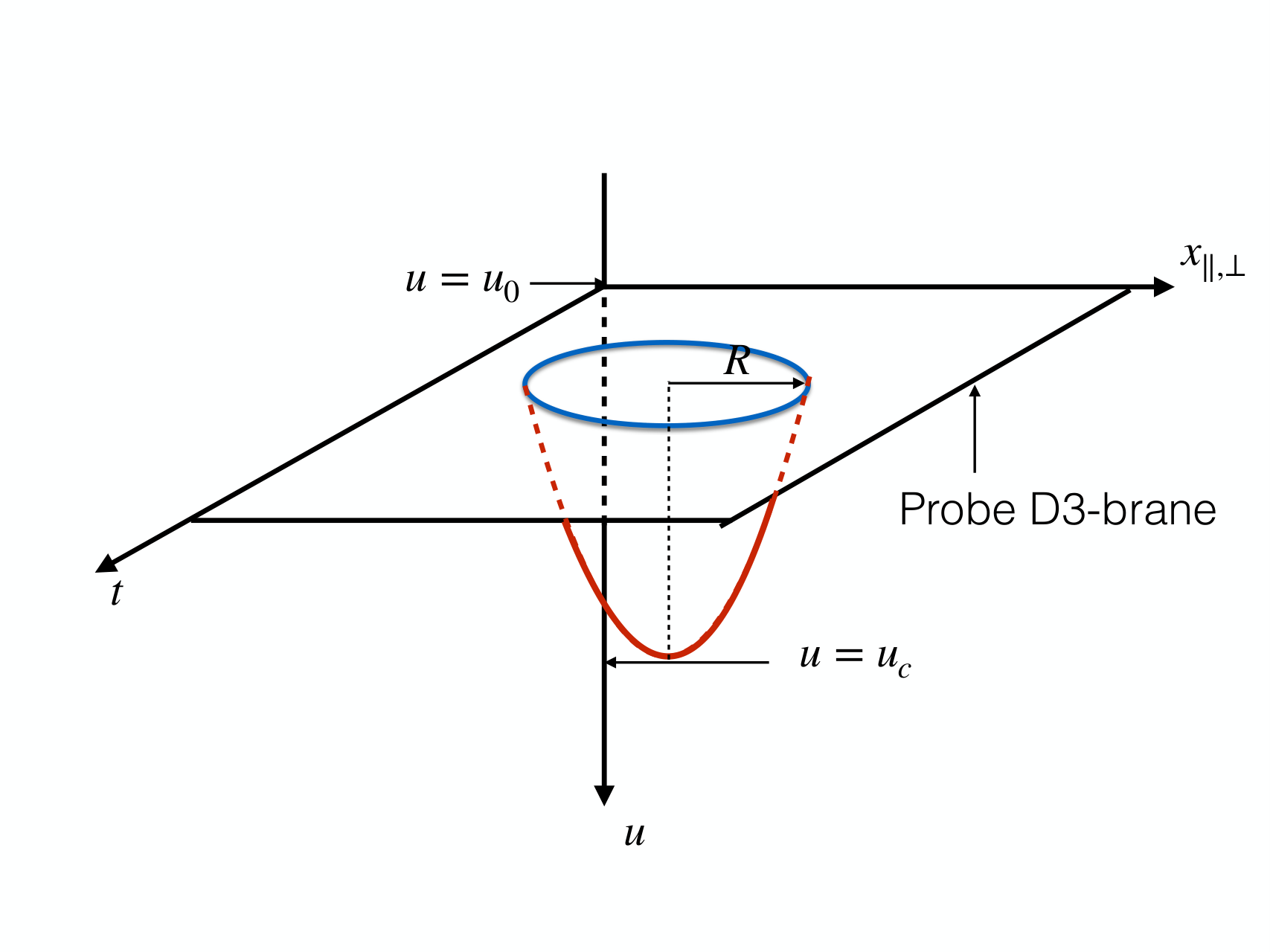
Since our concern is the radial dependence of string embedding, it would be convenient to choose the polar coordinates on the probe brane located at boundary as [12, 16, 18, 19]. However this would be a little tricky due to the anisotropy in the background geometry. To specify the derivation, let us first take into account the Wilson loop living in the plane of the probe D3-brane which is located at . Then impose the black brane solution with our notation , we can obtain the induced metric on plane as,
| (4.1) |
Hence the polar coordinates should be introduce as
| (4.2) |
so that
| (4.3) |
which reduces to a local coordinate transformation. Nonetheless, it is possible to evaluate the dependence of the anisotropy with this local coordinate transformation in holography since the asymptotic behavior of the background geometry near the holographic boundary is exactly same as the pure AdS spacetime i.e. . [20]. Therefore we can obtain the induced metric on the string world sheet with the polar coordinates given in (4.2) as,
| (4.4) |
where “” refers to . In this sense the NG action for such a fundamental string reads,
| (4.5) |
Then the equation of motion associated to action is given as,
| (4.6) |
which is expected to be solved numerically.
For the Wilson loop living in the plane, the NG action with our notation becomes,
| (4.7) |
where “” refers to and the local coordinate transformation is expected to be,
| (4.8) |
Then the associated equation of motion is obtained as,
| (4.9) |
In the bubble background, let us perform the above discussion again, then one may find the equation of motion for the fundamental string is as same as (4.6) and (4.9). Thus what we need to do next is to solve (4.6) and (4.9) numerically in order to evaluate the onshell action of the fundamental string. The boundary condition for (4.6) and (4.9) is illustrated in Figure 8 which is collected as,
| (4.10) |
Besides, the embedding function must satisfy the constraint as it is given in [15]. Accordingly, in our anisotropic system, for the Wilson loop living in the plane, the constraint is,
| (4.11) |
For the Wilson loop living in the plane, the constraint is,
| (4.12) |
Altogether, it would be possible to find a numerical solution for (4.6) (4.9) with the boundary condition (4.10) and the constraints (4.11) (4.12).
Afterwards, the pair production rate can be evaluated from the total onshell action of a fundamental string, which is given as
And the behavior of , as a function of , is numerically computed in Figure 9.
Our numerical calculation displays when the electric field is parallel (i.e. the case that the Wilson loop living in the plane), the pair production rate is increased by the anisotropy. However the pair production rate behaves oppositely in the perpendicular case (Wilson loop living in the plane). Interestingly, this conclusion seemingly agrees with the potential analysis in section 3. Since the potential barrier decreases/increases in the parallel/perpendicular case by the anisotropy, the production rate increases/decreases correspondingly in the parallel/perpendicular case.
5 Involving the flavor brane
As most works about D3-D7 approach, it is possible to investigate the involvement of flavors when a stack of probe flavor D7-branes is introduced into the bulk. In this section, we will briefly outline the embedding of the flavor D7-branes, then derive the effective flavored Lagrangian in dual theory, study the vacuum decay rate for the Schwinger effect and finally take a look at the V-A curve in this holographic system.
5.1 The effective Lagrangian
To begin with, let us introduce a probe D7-brane to the bulk. While there are different constructions to embed D7-brane as flavor in the IIB supergravity background, in this work we would consider the most widely used configuration of the flavor D7-brane embedding, that is the flavor D7-brane is parallel to the D3-branes. The D-brane configuration with respect to the black brane and bubble background is illustrated in Table 3 and 4.
| Black brane background | 0 | 1 | 2 | 3 | 4 | 5 | 6 | 7 | 8 | 9 |
|---|---|---|---|---|---|---|---|---|---|---|
| D3-brane | - | - | - | - | ||||||
| D7-brane | - | - | - | - | - | - | - | - | ||
| flavor D7-brane | - | - | - | - | - | - | - | - |
| Bubble background | 0 | 1 | 2 | 3 | 4 | 5 | 6 | 7 | 8 | 9 |
|---|---|---|---|---|---|---|---|---|---|---|
| D3-brane | - | - | - | - | ||||||
| D7-brane | - | - | - | - | - | - | - | - | ||
| flavor D7-brane | - | - | - | - | - | - | - | - |
According to the gauge-gravity duality, the hypermultiplet is excited due to the oscillations of an open string connecting the color (D3) and flavor (D7) branes, thus the massless/massive state corresponds to the configuration that D7-brane is touched/untouched to the stack of D3-branes, which is the content in the low-energy theory. Therefore the dual theory will contain the dynamics of flavors when the action of the flavor brane is taken into account. So the effective Lagrangian for dual theory is given by the bosonic action for the flavor D7-brane as99 9 While there should be a Wess-Zumino term in the D-brane action, it is vanished according to the supergravity solution in Section 1.,
| (5.1) |
where runs over the flavor brane, is the tension of the D7-brane, refers to the induced metric and is the gauge field strength on the flavor brane. By picking up the black brane background (2.2), we can obtain the induced metric on the flavor D7-brane as,
| (5.2) |
When the bubble background (2.5) is imposed, the induced metric on the flavor D7-brane becomes,
| (5.3) |
In addition, we need to turn on the external electric fields to evaluate electric features in dual theory as [24, 25, 26, 27]. Due to the anisotropy in the background geometry, we set the nonzero components of the gauge field strength as for the case that the electric field is parallel to the D7-branes in both backgrounds. For the case that the electric field is perpendicular to the D7-branes, we turn on the components of the gauge field strength as in the black brane background. Notice that in the perpendicular case, the nonzero components of the gauge field strength should be in the bubble background since the anisotropy is exhibited by of the metric. Here we use to refer to the homogeneous external electric field. Keeping these in hand, the effective action (5.1) could be written as, in the black brane background,
| (5.4) |
where,
| (5.5) |
And in the bubble background, the effective action (5.1) becomes,
| (5.6) |
where refers to the size of the compatified direction and,
| (5.7) |
5.2 The electric instability and vacuum decay rate
The electric instability and vacuum decay rate can be studied by analyzing the effective Lagrangian in dual theory since it may relate to the vacuum-to-vacuum amplitude [24] as,
| (5.8) |
where refers to the time-evolution operator with external fields, represents the spatial volume and refers to the vacuum state without external fields. So if the effective Lagrangian includes an imaginary part as 1010 10 For example, QED has the imaginary part of its Lagrangian up to 1-loop order as, which relates to a single quantum tunneling process in Schwinger effect where a pair of an electron and a positron is created from the vacuum.,
| (5.9) |
could be interpreted as the the vacuum decay rate. Accordingly, in order to evaluate the vacuum decay rate for the Schwinger effect, we need to derive the imaginary part of the effective Lagrangian with external electric fields presented in (5.4) (5.6) via holography. To achieve this goal, the equations of motion for the gauge field on the flavor brane are necessary which are 1111 11 The non-vanished components of the gauge field potential can be set as ., in the black brane background,
| (5.10) |
Since nothing depends on or in (5.10), it leads to and two constants defined as,
| (5.11) |
which is recognized as the electric charge and current . Plugging (5.11) back into (5.5) with respect to the case of “” and “”, we can obtain,
| (5.12) |
in the black brane background. Remarkably, for any stable configuration, it demands since the action (5.4) contains a factor . However, general choice of may lead to negative quantities for . Thus it implies there must be a critical position where the denominator and numerator in change their sign together. Then recall (5.8) (5.9) and suppose the electric field is turned on at suddenly, the original vacuum without electric current () would become unstable under the external electric field . Therefore the factor could not be real in the region which leads to an imaginary part of the effective Lagrangian as,
| (5.13) |
corresponding to the vacuum decay rate . And the critical position is determined by constraining (5.12), for parallel case, as
| (5.14) |
For perpendicular case, is determined by,
| (5.15) |
Using (5.13), the behavior of as a function of is plotted numerically in Figure 10 and 11 by solving the constraint of and in (5.14) (5.15).
Our numerical calculation displays the vacuum decay rate is a monotonic function of which agrees with the intuition that strong electric field would induce instability. On the other hand, as the analytical formulas of describes the situation of high temperature in the dual theory which is expected to be (like) deconfined quark-gluon plasma, thus there would not be a definitely critical value of the electric field for the Schwinger effect in conductive plasma. In addition, this holographic approach reveals that the vacuum decay rate would be increased/decreased by the presence of anisotropy with respect to parallel and perpendicular electric field . And this conclusion remains to agree with the potential analysis in Section 3 and the behaviors of the pari production rate given in Section 4.
Similarly, when the bubble background is picked up, the equations of motion for the gauge field strength can be obtained by varying action (5.6), then the electric charge and current can be achieved by their equations of motions as they are in (5.10) (5.11). As a result, the exact formula for in the bubble background is computed as follows,
| (5.16) |
Therefore the critical position must be determined by the constraints,
| (5.17) |
in the parallel case and,
| (5.18) |
in the perpendicular case. Afterwards, the vacuum decay rate can be obtained by evaluating the imaginary part of the effective Lagrangian in (5.6) which is given as,
| (5.19) |
Solving the constraint of and in (5.17) (5.18), we plot out the behavior of in (5.19) as a function of in Figure 12 and 13.
Obviously, the numerical calculation shows us a critical value of electric field when the bubble background is imposed which is distinct to the calculations in the black brane background. The reason is that the bubble background as a soliton solution corresponds to the confinement in the dual theory [30, 32]. So due to the confinement below , there should not be agreement with the calculations in the black brane background at small . Besides, Figure 12 and 13 also displays the similar behavior of the vacuum decay rate depending on the anisotropy as the black brane case, so it again agrees with our holographic investigation in Section 3 and 4.
5.3 The V-A curve
In this section, let us study the V-A curve in this holographic system. Since the relation of charge , current , critical position and the electric field is constrained by (5.14) (5.15) (5.17) (5.18), we solve these equations numerically and respectively by eliminating in order to obtain the relation of current and electric field . The numerical results are collected in Figure 14 and 15 in which the stable electric current is a function of the electric field with various and fixed .
We can see both in the black brane and bubble side, the behavior of the conductivity trends to become constant at large electric field which reveals the feature of DC conductor. And the presence of the anisotropy increases/decreases respectively which is in qualitative agreement with the phenomenologically holographic approach in this anisotropic background [28]1212 12 Notice that the notation of “” and “” in our manuscript is opposite to them in [28]. In our manuscript, “” and “” refer to that the physical variables is parallel/perpendicular to the dissolved D7-branes in the bulk while they refer to the variables is parallel/perpendicular to the anisotropic direction in [28].. However at small , our system is nearly insulated with charge density in bubble side which is consistent with its feature of confinement.
6 Summary and discussion
In this work, we study the Schwinger effect and vacuum electric instability in the anisotropic IIB supergravity via holography. In gravity side, two anisotropic gravity solutions are taken into account which are respectively the black brane solution and the bubble solution (as the soliton solution in gravity theory). The dual theory in the black brane background is analyzed at finite temperature while it is expected to be a three-dimensional confining theory at zero temperature in the bubble background. Using the AdS/CFT dictionary, we derive the critical electric field, the separation, the behavior of the holographic potential and the associated quark pair production both in the the black brane and the bubble background. However due to the anisotropy in the background, we also deal with the derivation in the parallel and perpendicular case respectively. Furthermore, when the D7-brane as flavor is introduced to the bulk geometry, it is possible to investigate the vacuum electric instability and the vacuum decay rate for Schwinger effect by calculating the imaginary part of the effective Lagrangian. In this sense, we solve the constraints of the charge, current, electric field then obtain the V-A curve and the conductivity in this holographic system. Since the analytical formulas of the background geometry is imposed, our calculation is valid in the limit of high temperature (black brane case), or in the exactly three-dimensional confining theory (bubble case).
Overall, our numerical calculation displays consistent results. First, for fixed electric field, the potential analysis reveals the potential barrier in parallel case is suppressed by the anisotropy while it is enhanced in the perpendicular case. And this behavior is in partly qualitative agreement with the numerical evaluation in the bottom-up holographic approach of the anisotropic Schwinger effect in [22]. Correspondingly, in our current work, the associated quark production rate increases/decreases in the parallel/perpendicular case, since potential barrier always hinders the pair production. And this conclusion agrees with the behavior of the quark potential in our anisotropic background studied in [21], in which the quark tension increases/decreases by the presented anisotropy in the perpendicular/parallel case. Second, when the flavor brane is introduced, we find that while the vacuum decay rate behaves differently at small electric field, it indicates similar behaviors of the dependence on the anisotropy as the quark production rate in the perpendicular/parallel case respectively. So we believe this is a parallel approach to verify the dependence on the anisotropy of the production rate via holography. Finally the V-A curve shows us a straightforward conclusion that is is always smaller than one with the anisotropy. This conclusion is in qualitative agreement with the phenomenologically holographic approach [28] in this system due to the interpretation of the transport property of anisotropic matters.
Additionally, in this framework, we can obtain the ratio of the perpendicular and parallel pressure in the dual theory is also smaller than one i.e. according to (2.13) or [20] at very high temperature or in the associated three-dimensional confining theory. Comparing with , it may lead to the statement that the pressure in very hot plasma or dense three-dimensional QCD may be roughly proportionally related to the conductivity. Afterwards combining the above conclusions together, we may find a consistent interpretation for the behaviors of the holographic potential and conductivity: Under the condition with anisotropy, the parallel direction may be more conductive than the perpendicular direction due to (i.e. the conductivity in the perpendicular/parallel direction is decreased/increased by the anisotropy respectively). Accordingly, it implies the virtual pairs of charged particles would be easier to be pulled apart to become real charged particles in the parallel direction than in the perpendicular direction under an external electric field. Therefore, the Schwinger effect with parallel electric field would be more likely to appear than with perpendicular electric field intuitively due to the presence of the anisotropy, which is embodied consistently as that the barrier of the holographic potential is decreased/increased with parallel/perpendicular electric field by the anisotropy because the potential barrier always hinders the Schwinger effect. In this sense, all the behaviors of the holographic potential in the presence of the anisotropy are basically due to the anisotropic bulk metric in our holographic setup. Thus we believe this holographic approach could provide a very powerful way to explore the non-perturbative Schwinger effect in the presence of anisotropy.
Acknowledgements
We would like to thank Xun Chen and Jing Zhou for helpful discussion. This work is supported by the National Natural Science Foundation of China (NSFC) under Grant No. 12005033, the research startup foundation of Dalian Maritime University in 2019 under Grant No. 02502608 and the Fundamental Research Funds for the Central Universities under Grant No. 3132022198.
Appendix: The analytical formulas for the anisotropic background
In general, the functions presented in (2.2) and (2.5) are non-analytical functions which must be determined by the equations of motion associated to the supergravity action (2.1). The details to solve numerically can be reviewed in [20]. Here we only collect the relevant formulas used in this work. We focus on the analytical formulas of which can be obtained in the high temperature limit , or in the black brane solution (2.2) as (up to the leading order terms of ),
| (A-1) |
where
| (A-2) |
Here refers to the event horizon in the black brane solution. We note that the functions in (A-1) ( A-2) are in fact a series of once the relation of and is imposed. So the high temperature analysis of refers to the condition in the original solution exactly.
Since the bubble background (2.5) is obtained under the double Wick rotation, it would reduce to the replacement where refers to the period of . Note that in the bubble background we would replace by because it now refers to the bottom of the Cigar-like bulk instead of a horizon. In this sense, the high temperature limit , or in the original black brane solution corresponds to the limit of dimension reduction or in the bubble solution. Namely, in this limit, the size of the compactified direction trends to be zero in (2.5). In a word, by replacing by , if we remain to employ analytical formulas of given in (A-1) (A-2) in the bubble background, the dual theory is effectively three-dimensional below with which means the dual theory would become exactly a three-dimensional theory. And in this work, we use the above formulas for functions , thus it means all our calculations are valid with the anisotropy of under the condition .
References
- [1] J. Schwinger, “On gauge invariance and vacuum polarization,” Phys. Rev. 82 (1951) 664.
- [2] I. Affleck, O. Alvarez and N. S. Manton, “Pair Production At Strong Coupling In Weak External Fields,” Nucl. Phys. B 197 (1982) 509.
- [3] E. Shuryak, “Why does the quark gluon plasma at RHIC behave as a nearly ideal fluid?”, Prog.Part.Nucl.Phys. 53 (2004) 273-303, arXiv:hep-ph/0312227.
- [4] E. Shuryak, “What RHIC experiments and theory tell us about properties of quark-gluon plasma? ”, Nucl.Phys.A 750 (2005) 64-83, arXiv:hep-ph/0405066.
- [5] W. Florkowski, R. Ryblewski, “Highly-anisotropic and strongly-dissipative hydrodynamics for early stages of relativistic heavy-ion collisions”, Phys.Rev.C 83 (2011) 034907, arXiv:1007.0130.
- [6] R. Ryblewski, W. Florkowski, “Non-boost-invariant motion of dissipative and highly anisotropic fluid”, J.Phys.G 38 (2011) 015104, arXiv:1007.4662.
- [7] M. Martinez, M. Strickland, “Dissipative Dynamics of Highly Anisotropic Systems”, Nucl.Phys.A 848 (2010) 183-197, arXiv:1007.0889.
- [8] M. Martinez, M. Strickland, “Non-boost-invariant anisotropic dynamics”, Nucl.Phys.A 856 (2011) 68-87, arXiv:1011.3056.
- [9] O. Aharony, S. S. Gubser, J. M. Maldacena, H. Ooguri and Y. Oz, “Large N field theories, string theory and gravity”, Phys. Rept. 323 (2000) 183, arXiv:hep-th/9905111.
- [10] E. Witten, “Anti-de Sitter space and holography”, Adv.Theor.Math.Phys. 2 (1998) 253-291, arXiv:hep-th/9802150.
- [11] G. Semenoff, K. Zarembo, “Holographic Schwinger Effect”, Phys.Rev.Lett. 107 (2011) 171601, arXiv:1109.2920.
- [12] Y. Sato, K. Yoshida, “Potential Analysis in Holographic Schwinger Effect”, JHEP 08 (2013) 002, arXiv:1304.7917.
- [13] Y. Sato, K. Yoshida, “Universal aspects of holographic Schwinger effect in general backgrounds”, JHEP 12 (2013) 051, arXiv:1309.4629.
- [14] Y. Sato, K. Yoshida, “Holographic Schwinger effect in confining phase”, JHEP 09 (2013) 134, arXiv:1306.5512.
- [15] Y. Sato, K. Yoshida, “Holographic description of the Schwinger effect in electric and magnetic fields”, JHEP 04 (2013) 111, arXiv:1303.0112.
- [16] D. Kawai, Y. Sato, K. Yoshida, “Schwinger pair production rate in confining theories via holography”, Phys.Rev.D 89 (2014) 10, 101901, arXiv:1312.4341.
- [17] M. Ghodrati, “Schwinger Effect and Entanglement Entropy in Confining Geometries”, Phys.Rev.D 92 (2015) 6, 065015, arXiv:1506.08557.
- [18] L. Shahkarami, M. Dehghani, P. Dehghani, “Holographic Schwinger Effect in a D-Instanton Background”, Phys.Rev.D 97 (2018) 4, 046013, arXiv:1511.07986.
- [19] S. Li, “Holographic Schwinger effect in the confining background with D-instanton”, Eur.Phys.J.C 81 (2021) 9, 797, arXiv:2005.11955.
- [20] D. Mateos, D. Trancanelli, “Thermodynamics and Instabilities of a Strongly Coupled Anisotropic Plasma”, JHEP 07 (2011) 054, arXiv:1106.1637.
- [21] S. Li, S. Luo, Y. Hu, “Holographic QCD and Chern-Simons theory from anisotropic supergravity”, JHEP 06 (2022) 040, arXiv:2203.14489.
- [22] J. Zhou, J. Chen, L. Zhang, J. Ping, X. Chen, “Holographic Schwinger Effect in Anisotropic Media”, arXiv: 2101.08105.
- [23] A. Karch, E. Katz, “Adding flavor to AdS / CFT”, JHEP 0206 (2002) 043, arXiv:hep- th/0205236.
- [24] K. Hashimoto, T. Oka, “Vacuum Instability in Electric Fields via AdS/CFT: Euler-Heisenberg Lagrangian and Planckian Thermalization”, JHEP 1310 (2013) 116, arXiv:1307.7423.
- [25] K.Hashimoto, T. Oka, A. Sonoda, “Magnetic instability in AdS/CFT: Schwinger effect and Euler-Heisenberg Lagrangian of supersymmetric QCD”, JHEP 06 (2014) 085, arXiv:1403.6336.
- [26] K.Hashimoto, T. Oka, A. Sonoda, “Electromagnetic instability in holographic QCD”, JHEP 06 (2015) 001, arXiv:1412.4254.
- [27] W. Cai, K. Li, S. Li, “Electromagnetic instability and Schwinger effect in the Witten–Sakai–Sugimoto model with D0–D4 background”, Eur.Phys.J.C 79 (2019) 11, 904, arXiv:1612.07087.
- [28] A. Rebhan, D. Steineder, “Violation of the Holographic Viscosity Bound in a Strongly Coupled Anisotropic Plasma”, Phys.Rev.Lett. 108 (2012) 021601, arXiv:1110.6825.
- [29] R. Janik, P. Witaszczyk, “Towards the description of anisotropic plasma at strong coupling”, JHEP 09 (2008) 026, arXiv:0806.2141.
- [30] E. Witten, “Anti-de Sitter space, thermal phase transition, and confinement in gauge theories”, Adv. Theor. Math. Phys. 2 (1998), 505-532, arXiv:hep-th/9803131.
- [31] I. Papadimitriou, “Holographic Renormalization of general dilaton-axion gravity”, JHEP 08 (2011) 119, arXiv: 1106.4826.
- [32] K. Becker, M. Becker, J. Schwarz, “String Theory and M-Theory, A Modern Introduction”, Cambridge University Press, Cambridge, 2007.
- [33] J. Maldacena, “Wilson loops in large N field theories”, Phys.Rev.Lett. 80 (1998) 4859-4862, arXiv:hep-th/9803002.