Nonparametric inference under a monotone hazard ratio order
University of Massachusetts Amherst
August 11, 2026
Abstract
The ratio of the hazard functions of two populations or two strata of a single population plays an important role in time-to-event analysis. Cox regression is commonly used to estimate the hazard ratio under the assumption that it is constant in time, which is known as the proportional hazards assumption. However, this assumption is often violated in practice, and when it is violated, the parameter estimated by Cox regression is difficult to interpret. The hazard ratio can be estimated in a nonparametric manner using smoothing, but smoothing-based estimators are sensitive to the selection of tuning parameters, and it is often difficult to perform valid inference with such estimators. In some cases, it is known that the hazard ratio function is monotone. In this article, we demonstrate that monotonicity of the hazard ratio function defines an invariant stochastic order, and we study the properties of this order. Furthermore, we introduce an estimator of the hazard ratio function under a monotonicity constraint. We demonstrate that our estimator converges in distribution to a mean-zero limit, and we use this result to construct asymptotically valid confidence intervals. Finally, we conduct numerical studies to assess the finite-sample behavior of our estimator, and we use our methods to estimate the hazard ratio of progression-free survival in pulmonary adenocarcinoma patients treated with gefitinib or carboplatin-paclitaxel.
1 Introduction
1.1 Background and literature review
Time-to-event data are commonplace in many scientific fields, including biomedicine, economics, and engineering. In many circumstances, interest focuses on comparing the distribution of the time it takes for some event to occur, known as the event time, in two populations. For instance, in the medical sciences, patients may be randomly assigned to treatment or control, and followed until an event of interest occurs, such as onset, recurrence, or cure of a disease. In this case, the two populations are patients randomized to treatment and patients randomized to control. While the methods discussed in this paper are applicable to any time-to-event data, we will use “patients” to refer to the units in the population of interest for convenience.
In the analysis of time-to-event data, one common parameter of interest is the cumulative distribution function of the event time, or equivalently, its survival function. However, in many settings, the event time is not observed for all patients in the study because, for example, some patients may prematurely leave the study, or the event may not have occurred before the end of the study period. This is known as right-censoring of the event time. If the censoring process is independent of the event process, the Kaplan-Meier estimator (Kaplan and Meier 1958) is a consistent nonparametric estimator of the survival function of the event time.
The distribution and survival functions describe cumulative probabilities, but in some cases it is of interest to quantify the instantaneous rate of the event at a point in time among patients who have not yet experienced the event of interest. This is known as the hazard rate. When comparing the distributions of an event time in two populations, the ratio of the hazard rates, known as the hazard ratio, describes the relative event rates among patients who have not yet experienced the event in the two populations over time. Estimating the hazard rate or ratio is more difficult than estimating the survival function because the hazard rate and ratio concern events occurring in an infinitesimal window of time. However, estimation of the hazard ratio is made much simpler by assuming that it is constant in time, which is known as the proportional hazards assumption. When this assumption holds, Cox proportional hazards regression can be used to estimate the hazard ratio (Cox 1972). In this case, the hazard ratio for comparing two populations reduces to a single number. The hazard ratio estimated from a simple Cox regression comparing two populations has become one of the most important tools in the analysis of time-to-event data, and in some studies it is the only effect reported (Hernán 2010).
Despite the widespread use of Cox regression, the proportional hazards assumption underlying it is easily violated. For example, if a treatment only offers short-term benefits over control, then the hazard ratio is unlikely to be constant (Li et al. 2015). In addition, the proportional hazards assumption implies that the survival function of one group can be expressed as the survival function of the other group raised to a constant power. Hence, if the survival curves cross, then the proportional hazards assumption cannot hold (see, e.g. Klein and Moeschberger 2003). The hazard ratio estimated by a Cox regression in a setting where the proportional hazards assumption is violated is approximately a weighted average of the hazard ratio function over time (Struthers and Kalbfleisch 1986). However, the weighting function depends on the censoring pattern in the study, which complicates the interpretation of the parameter estimated by the Cox model in such a misspecificed model (O’Quigley 2008; Whitney et al. 2019)
When the proportional hazards assumption is violated, estimating the hazard ratio function is more difficult. One simple approach is to estimate the hazard ratio using the ratio of estimators of the individual hazard rate functions. For example, if correctly specified parametric models for the distributions are available, the hazard rates in the two distributions can be estimated using maximum likelihood estimation (Kalbfleisch and Prentice 2011). Alternatively, nonparametric methods for estimating hazard functions based on smoothing have also been proposed (Anderson and Senthilselvan 1980; Müller and Wang 1994; Rebora et al. 2014). However, estimators based on smoothing are often sensitive to the selection of certain tuning parameters, such as bandwidths, kernel functions, or the number of knots in a spline function. In addition, obtaining valid inference using a smoothing-based estimator can be challenging due to bias in the asymptotic distribution of the estimator (see, e.g. Wasserman 2013 and Calonico et al. 2018).
In some cases, it may be known that the hazard ratio is monotone as a function of time. In general, the hazard ratio can be expected to be monotone when the relative rate of events in the two groups increases or decreases over time. For example, if the effectiveness of a treatment wanes over time, then the hazard ratio between treated and placebo groups of a randomized trial may be expected to be monotone non-decreasing (Durham et al. 1998). Similarly, harmful exposures can result in a monotone non-decreasing hazard ratio between the exposed and unexposed groups (Sekula et al. 2013). We discuss the motivation and application of monotone hazard ratios more in Section 2.
We are only aware of a few studies concerning monotonicity of the hazard ratio function. Gill and Schumacher 1987 and Deshpande and Sengupta 1995 proposed tests of the proportional hazards assumption against the non-decreasing hazard ratio alternative. Kim et al. 2011 proposed an estimator of a monotone hazard ratio function using a nonparametric Bayesian approach, which we discuss further in Section 3.
1.2 Contribution and organization of the article
In this article, we study the situation in which the hazard ratio between two populations is known to be non-decreasing in time. First, we define a new stochastic order called the monotone hazard ratio order, demonstrate that it is an invariant stochastic order in the sense of Lehmann and Rojo 1992, and study the properties of this novel stochastic order. As we will discuss more below, this is important because it gives stability to the monotonicity assumption, and because it connects our new order to the existing literature on stochastic orders. Second, we propose a novel estimator of a hazard ratio function under a monotonicity constraint in the presence of independent right-censoring. Finally, we derive the large-sample properties of our estimator, including convergence in distribution of our estimator at the rate to a mean-zero limit, and use this result to construct asymptotically valid pointwise confidence intervals for the hazard ratio function. To the best of our knowledge, we are the first to study the stochastic order defined by monotonicity of the hazard ratio function, and we are also the first to produce asymptotically valid confidence intervals for a monotone hazard ratio function.
The paper proceeds as follows. In Section 2, we define the monotone hazard ratio order and establish properties of this order. In Section 3, we introduce our nonparametric estimator of a monotone hazard ratio function, establish asymptotic theory of our estimator, and use this theory to construct confidence intervals. In Section 4, we present numerical studies evaluating the finite-sample performance of our method. Finally, in Section 5, we use our method to estimate the hazard ratio function comparing the length of progression-free survival of pulmonary adenocarcinoma patients treated with gefitinib or carboplatin-paclitaxel. Proofs of all theorems can be found in Supplementary Material.
1.3 Notation
For a function on a domain to the extended real line , we let . If possesses limits from the left, then we let be the left-continuous version of , and if possesses limits from the right, then we let be the right-continuous version of . We set . If is left-differentiable at , we denote by the left derivative of at . We also denote the image of by for some . If is non-decreasing, we define the support of as for all . We define the greatest convex minorant (GCM) of on , denoted , as the pointwise supremum of all convex functions on bounded above by . We say that is monotone on if for all with , and similarly we say that is convex on if for all and such that as well. We set as the generalized inverse function corresponding to . The properties of such functions when is a distribution function (in which case is its quantile function) are summarized in Chapter 21 of van der Vaart 2000. All integrals should be interpreted as Riemann-Stieltjes integrals, and by default.
2 Monotone hazard ratio ordering
2.1 Definition of the monotone hazard ratio order
We now introduce and motivate the monotone hazard ratio order. We let and be nonnegative random variables, and we let , , , and be the distribution and survival functions corresponding to and , respectively. If and are absolutely continuous with density functions and , then and are the hazard functions corresponding to and , respectively. In this case, we say if is non-decreasing for such that or . On the other hand, if and are fully discrete random variables with support contained on a finite or countably infinite set , then and are the corresponding hazard functions, where and are the corresponding mass functions (and where ). In this case, we say if is non-decreasing for all such that or .
We define in such a way that encompasses both the above cases, as well as more complicated cases where and may be mixed discrete-continuous random variables. We let be any sigma-finite measure dominating both and , and we define and . We then define the hazard functions relative to as on the support of , and 0 otherwise, and similarly for . The hazard ratio function is then defined as . We note that does not depend on the choice of dominating measure , that on , and that on . We then have the following general definition of the monotone hazard ratio relation.
Definition 1.
We say that if is non-decreasing on .
When both and are dominated by Lebesgue measure, we recover the first case discussed above, and when they are both dominated by counting measure on the countable set , then we recover the second case.
Monotone hazard ratios abound in the literature because monotonicity of hazard ratio function can be expected to hold in several general situations. First, if is the time to an adverse event under treatment and is the same under control, we can expect if the protective effect of the treatment on those who have not yet experienced it wanes over time. There are many examples of such treatments, including vaccines (Durham et al. 1998) and blood transfusion (Holcomb et al. 2013). Second, if is the time to an adverse event under control, and is the same under exposure to a condition with short-term toxic effects, then we may again expect that . Drug overdose is an example of such a toxic exposure (Hernandez et al. 2018). We note that the individual hazard functions of and may not be monotone in the above cases. For instance, there may be underlying time trends (e.g., weekly, monthly, or seasonal trends) unrelated to treatment that induce non-monotonic trends in the hazards. If these trends influence the hazards of and equally, then the hazard ratio may still be expected to be monotone.
The statistical model induced by the monotone hazard ratio order is a generalization of the popular proportional hazards model with a time trend, where the time trend is allowed to be any monotone function. Choosing a specific time trend for a proportional hazards model can be difficult, and if the time trend is chosen based on the data, obtaining valid inference for the regression coefficient is challenging (Desquilbet and Meyer 2005). Hence, the flexibility in permitting any monotone time trend is appealing because it avoids the need to choose a specific trend.
We will see in Section 3 that when it is known that the hazard ratio is monotone, this knowledge can be exploited to obtain a simple nonparametric estimator of the hazard ratio function and asymptotically valid pointwise inference. Furthermore, the estimator and inferential procedure avoid estimating or modelling the individual hazard functions directly, in the same spirit as the proportional hazards estimator, which yields improved robustness over methods that estimate the hazard functions. This will be explored more in numerical studies in Section 4.
2.2 Properties of the monotone hazard ratio order
We now establish several important properties of the monotone hazard ratio order. First, we show that the relation defined above is an invariant stochastic order in the sense of Lehmann and Rojo 1992. Intuitively, stochastic orders are ways of defining what it means for one probability distribution to be “larger” than another. Specifically, a stochastic order is a relation on the space of probability distributions on some measurable space satisfying the conditions of a preorder: for any probability distributions , , and on the space, (1) , and (2) and implies that . We will be focused on distributions on the reals. In this case, a stochastic order is invariant under monotone transformations, or simply invariant, if implies for any strictly increasing continuous function with and . For two real-valued random variables and with distribution functions and , we say for a stochastic order if . We now show that these properties hold for the monotone hazard ratio order defined above.
Theorem 1.
(1) For any random variable , ; (2) for any , , and such that and , it holds that ; and (3) for any strictly increasing continuous function with and , implies that .
The fact that the monotone hazard ratio forms a stochastic order is important due to the stability it provides when comparing the hazard ratios of multiple event times. The fact that it is invariant to monotone transformations is especially important because it means that the order is independent of time scale. We also note that and implies that the hazard ratio is constant, but does not imply that in distribution. Hence, the monotone hazard ratio order is not antisymmetric, and therefore does not induce a partial order.
We now provide two characterizations of the monotone hazard ratio order in the special case where , i.e. is dominated by . We define and as the cumulative hazard functions corresponding to and , respectively, and we note that if , then , and . We also define as the ordinal dominance curve corresponding to the distributions of and . Lehmann and Rojo 1992 demonstrated that all invariant stochastic orders are equivalent to a pre-order on the space of ordinal dominance curves that is closed under composition. In the next result, we provide two characterizations of the monotone hazard ratio order: one in terms of the ordinal dominance curve, and a second in terms of the cumulative hazard functions and .
Theorem 2.
(a) If and is continuous, then the following are equivalent:
- 1.
;
- 2.
is convex on ;
- 3.
is convex on .
(b) If , is continuous, and , then for any , where is the smallest closed interval containing .
The assumption that is important for the characterizations in Theorem 2. For example, if is the uniform distribution on and is the Bernoulli distribution with probability , then is not dominated by , but is convex on and . This is similar to a counterexample provided in Mösching and Dümbgen 2020 for the likelihood ratio order. If treatment or exposure does not change the set of possible event times, which is the case in many real-world situations, then can be expected to hold.
The characterization of the monotone hazard ratio order in terms of the ordinal dominance curve provided in Theorem 2 is somewhat more complicated than the characterization of the other three common invariant stochastic orders discussed below. This is due to the complexity of the general relationship between a hazard function and the corresponding distribution function. In the case of absolutely continuous and , the characterization in terms of the ordinal dominance curve can be stated somewhat simpler. In particular, is convex if and only if is monotone, which holds if and only if is monotone. Then, since , in the absolutely continuous case the monotone hazard ratio order is equivalent to being log-convex on . In this case, it is necessary but not sufficient that be log-convex.
The relationship between the hazard and cumulative hazard functions is analogous to that between a density and distribution function. Hence, the characterization of the monotone hazard ratio order in terms of the cumulative hazard functions provided in Theorem 2 parallels the characterization of a likelihood ratio order in terms of the distribution functions (Westling et al. 2021; Mösching and Dümbgen 2020). We will see in Section 3 that part (b) of Theorem 2 suggests a natural estimator of .
Theorem 2 can also be used to informally assess the plausibility of the monotone hazard ratio order given data. We note that is convex on if and only if the parametrized curve is convex on . Hence, if and are consistent estimators of and , respectively, then if and only if is consistent for a convex function. Hence, comparing this curve to its GCM gives an informal graphical check of the monotone hazard ratio order. This same procedure was proposed by Gill and Schumacher 1987.
2.3 Relationship to other stochastic orders
A variety of stochastic orders have been studied; Shaked and Shanthikumar 2007 contains detailed results and discussion. We briefly review three of the most common stochastic orders used in the context of univariate time-to-event analysis. The usual or uniform stochastic order is defined as if for all , where and are cumulative distribution functions on . Estimators under the usual stochastic order were developed by Brunk et al. 1966 and Dykstra 1982, and the corresponding asymptotic properties were derived by Præstgaard and Huang 1996. The hazard rate order is defined as if is non-increasing, which is equivalent to in the case of absolutely continuous distributions, where and are the densities corresponding to and . Dykstra et al. 1991 studied estimation and inference under a hazard rate order. Finally, the likelihood ratio order is defined as if is non-decreasing. Dykstra et al. 1995; Yu et al. 2017; Mösching and Dümbgen 2020 and Westling et al. 2021 considered estimation and inference under a likelihood ratio order. These three canonical examples of stochastic orders are themselves ordered: implies implies .
It is natural to ask where the monotone hazard ratio order fits into the hierarchy of the three common stochastic orders. It turns out that the monotone hazard ratio order does not generally imply, nor is it implied by, any of the three common stochastic orders. To show this, we provide continuous and discrete counterexamples for each case. These examples are illustrated in Figure 1. We note that the fact that our order is not implied by nor implies these other orders means in particular that previously established properties of and methods for inference under these orders do not apply to the monotone hazard ratio order.
We first show that the monotone hazard ratio order does not imply the usual stochastic order, which further implies that the monotone hazard ratio order does not imply the hazard rate or monotone likelihood ratio orders. Suppose that and have Weibull distributions with shape parameters and and scale parameters and , respectively. Then the hazard ratio function is proportional to for , so that if and only if , and if and only if . On the other hand, if and only if . If , then ranges from to , which implies that it cannot be the case that either or . Therefore, if , then , but , which also implies that and . Hence, the monotone hazard ratio order does not imply any of these other three common orders in the continuous case (first column of Figure 1). For a counterexample in the discrete case, suppose that follows a geometric distribution with success probability on , so that for all . Hence, for any supported on such that is non-increasing in . The usual stochastic order fails to hold if for any . Both of these are the case, for instance, if also follows a geometric distribution with success probability (second column of Figure 1).
We now show that the likelihood ratio order does not imply the monotone hazard ratio order, which further implies that the hazard rate order and usual stochastic order do not imply the monotone hazard ratio order. For an example in the continuous case, suppose that and follow Beta distributions with parameters and for . Then the density ratio is proportional to , which is strictly increasing, so . Furthermore, if , then one can also show that the hazard ratio function is strictly decreasing, so that . Therefore, the likelihood ratio order does not imply the monotone hazard ratio order in the continuous case, so neither do the hazard rate or usual stochastic orders (third column of Figure 1). For a counterexample in the discrete case, suppose has a uniform distribution on for and satisfies (1) for , and (2) for all . Both (1) and (2) can be achieved simultaneously if and only if . Then the ratio of the mass functions is proportional to , so the likelihood ratio order holds by assumption (1). However, we can also show that for all . So the monotone hazard ratio order cannot hold (last column of Figure 1).

One special case where the monotone hazard ratio order does imply the hazard rate order, and therefore the usual order as well, is when , where . This is the case, for instance, when a treatment is known to be non-toxic, or when a harmful exposure is known to never be beneficial. In particular, if and are supported on the same finite discrete set and and , then necessarily so implies .
3 Nonparametric inference with right-censored data
3.1 Statistical setting
In this section, we provide an estimator of a monotone hazard ratio function using independently right-censored data. We derive the asymptotic distribution of our estimator, and use this result to construct asymptotically valid pointwise confidence intervals for .
For each , we let indicate the cohort for unit . For a randomized study, corresponds to control, and corresponds to treatment, though the data need not be from a randomized trial. We assume that . For such that , we let be the event time and be the censoring time. For such that , we let be the event time and be the censoring time. We assume that and are independent and and are independent for each — that is, the censoring is independent of the event within each treatment arm. If , we observe the right-censored data and , and if , we observe and . The observed data for unit is then , and we assume that are IID.
When and are discrete, the hazard ratio function can be estimated using the ratio of the empirical hazard functions within each treatment arm. The empirical hazard functions converge at the rate to normal limits, so by the delta method, their ratio does as well. Hence, inference for the hazard ratio function in this case can be obtained using standard methods. Furthermore, monotonicity of the hazard ratio function can be enforced by projecting the empirical estimator onto the space of monotone functions (Westling et al. 2020b). Therefore, here, we focus on the more challenging case where and are absolutely continuous distributions. We make no assumptions about the censoring distributions and .
3.2 Proposed estimator
Our estimator is based on the representation of presented in Theorem 2. We recall from Theorem 2 that if and is non-decreasing and continuous on the support of , then we can represent in terms of the cumulative hazard functions and as , where is the smallest closed interval containing . Our estimator is defined by replacing the unknown elements in this representation with nonparametric estimators thereof. We let be the stratified Nelson-Aalen estimator (Nelson 1969; Aalen 1978) of the cumulative hazard function based on the cohort for which . Similarly, we let be the stratified Nelson-Aalen estimator of based on the control cohort for which . We also define , where is the minimum of the empirical quantile of the ’s for which and the empirical quantile of the ’s for which , where is a non-increasing sequence converging to . It follows that is converging to , the minimum of the th quantile of given and the th quantile of given . Additional conditions on and practical suggestions for setting will be provided below. We then define our estimator of as
It is straightforward to compute using standard software packages. Specifically, in the statistical computing software R (R Core Team 2021), the Nelson-Aalen estimators can be obtained using the package survival (Therneau 2022), and the slopes of the greatest convex minorant of can be obtained using the package fdrtool (Strimmer 2008). Code for computing is provided in Supplementary Material.
Kim et al. 2011 proposed a nonparametric Bayesian approach to estimating a monotone hazard ratio function. Their model permits either monotone non-decreasing or non-increasing hazard ratio functions, whereas the type of monotonicity must be known a priori for our estimator. Their model also allows for the incorporation of covariates, which we have have not explored. However, approximating the posterior distribution in their model is complicated and possibly computationally intensive, in contrast to the simple implementation of our procedure.
3.3 Convergence in distribution
We now demonstrate that converges in distribution for fixed to a scaled Chernoff distribution. The (standard) Chernoff distribution is defined as the derivative at zero of the GCM of a Brownian motion plus a quadratic; i.e. , where for a standard two-sided Brownian motion with .
Theorem 3.
Suppose is such that that , , and are continuously differentiable at with finite and strictly positive derivatives, and , , , and are in a neighborhood of . Also suppose that there exist such that for all . Then
where follows the Chernoff distribution and
Due to its connection with GCMs, the Chernoff distribution appears in the asymptotic distribution of summaries of many monotonicity-constrained estimators (e.g., Groeneboom 1985; Huang and Wellner 1995; Westling et al. 2021, among many others). The properties of the Chernoff distribution were studied extensively by Groeneboom and Wellner 2001. In particular, common quantiles of the distribution are tabulated therein, which facilitates the construction of asymptotic confidence intervals for using Theorem 3, as we discuss below.
Theorem 3 implies that converges to at the rate . This is slower than the rate achieved by estimators of the hazard function based on kernel smoothing with optimal bandwidth selection (Müller and Wang 1990; Groeneboom et al. 2010). However, this latter result requires that the hazards possess two continuous derivatives, while Theorem 3 only requires one continuous derivative of the hazard ratio. In addition, asymptotically valid inference using estimators based on kernel smoothing is challenging due to bias arising in the limit distribution (Calonico et al. 2018).
Theorem 3 requires that not converge too quickly to zero, meaning that the upper limit of the region over which the GCM is taken not converge too quickly to the upper limit of support of the observed times. This ensures that and are uniformly consistent on the increasing interval (Stute 1994). The requirement is satisfied if, for instance, for all , or if for some . In practice, we recommend setting for , and for .
Kim et al. 2011 proposed a nonparametric Bayesian approach to estimating a monotone hazard ratio function. Their model permits either monotone non-decreasing or non-increasing hazard ratio functions. The type of monotonicity must be known a priori for our estimator, but we expect that in most cases where monotonicity can be assumed, the direction of monotonicity is also known. Approximating the posterior distribution in their model is complicated and possibly computationally intensive, in contrast to the simple implementation of our procedure. Kim et al. 2017 proved that the rate of convergence of the posterior distribution of the nonparametric Bayesian estimator proposed by Kim et al. 2011 is , which is just a poly-log factor slower than the rate of convergence of our estimator. However, to the best of our knowledge, it is not known whether the posterior distribution of the estimator proposed by Kim et al. 2011 yields asymptotically calibrated confidence intervals for . In the next section, we use Theorem 3 to construct asymptotically valid pointwise intervals using our estimator.
3.4 Construction of confidence intervals
We propose two methods of constructing confidence intervals for . The first method is based on the asymptotic distribution of provided in Theorem 3. By Theorem 3, a Wald-type asymptotic -level confidence interval for is given by , where is a consistent estimator of , and is the th quantile of the standard Chernoff distribution. Quantiles of the Chernoff distribution are tabulated in Groeneboom and Wellner 2001. We note that involves both and , so one approach to estimating would be to plug in consistent estimators of and . Instead, we rewrite as
This form of no longer depends directly on or . In this expression, , , and the Kaplan-Meier estimators , , , and can be substituted for their true counterparts in constructing an estimator of . Hence, the only remaining challenge is to estimate . We do this using the derivative estimator obtained by applying a local linear kernel smoother to the set of points , where , and is a uniform grid on . We choose the bandwidth for the kernel smoother using cross validation (Guidoum 2020).
Sample splitting has also been shown to yield valid inference and reduced variance for estimators with -rate asymptotics without the need to estimate additional nuisance parameters in the limit distribution (Banerjee and Wellner 2005; Banerjee et al. 2019). To implement this method, the observations are first split randomly into disjoint subsets of approximately equal size. The estimator is then computed for each subset . These estimators are averaged to obtain a pooled estimator . Finally, an asymptotic -level confidence interval for is given by , where is the empirical standard deviation of the subset estimators and is the th quantile of the distribution with degrees of freedom.
4 Numerical studies
To assess the finite-sample performance of our proposed estimator and confidence intervals, we performed the following numerical study. We simulated data from three different scenarios corresponding to linear, convex, and concave . Defining , in the linear case, we set and , so that . In the convex case, we set and , so that . In the concave case, we set and , so that . Notably, and for all , and are multiples of a periodic function due to the inclusion of . This is common in many applications where event rates follow weekly, monthly, or seasonal trends. For the censoring distributions, we set both and as for , for , and for . Hence, the censoring distributions are mixed discrete-continuous distributions supported on , and have discrete components at 1 and 2 with probabilities 0.044 and 0.078, respectively. Finally, we set .

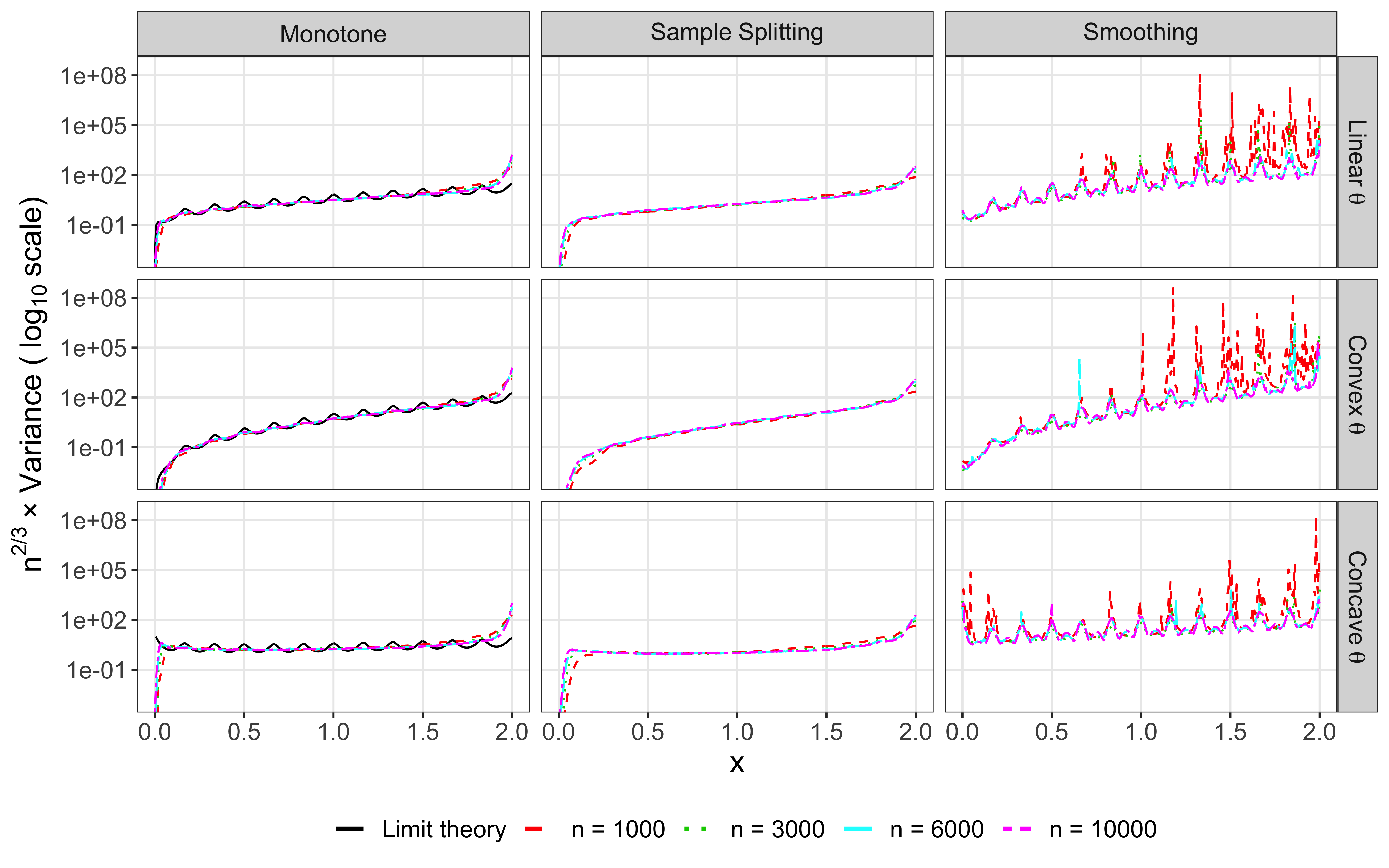
For each sample size equal to 1000, 3000, 6000, and 10000, we simulated 1000 right-censored datasets for each of the three mechanisms described above. For each dataset and for each equal to , we computed our proposed estimator , the sample splitting estimator with splits, and the corresponding confidence intervals defined in Section 3.4. For comparison, we also computed an estimator and confidence intervals based on taking the ratio of kernel smoothing estimators of the individual hazard functions, which does not require or enforce monotonicity of (Watson and Leadbetter 1964). For the kernel smoothing estimators of the hazard functions, we used the Epanechnikov kernel and selected the bandwidths using cross validation. We did not compare our procedure to that of Kim et al. 2011 due to the lack of availability of computer code implementing their procedure.
The top panel of Figure 2 displays times the absolute bias of the three estimators as a function of . Figure 6 in Supplementary Material displays the relative absolute bias of the smoothing and sample splitting estimators to our estimator. The scaled bias of all three estimators generally decreases with sample size, which aligns with the expectation that the biases decrease faster than for . The absolute bias of the three estimators exhibits periodicity inherited from the periodicity of the underlying hazard functions. All three estimators exhibit large bias near , which is expected given the challenges of estimation near the boundary of support. The bias near is highest for all three estimators in the concave case, and the bias for between 1 and 2 is largest in the convex case, which makes sense because this is when the derivative of is large.
For most values of , our estimator has slightly smaller absolute bias than the sample splitting estimator, especially for , which is expected because the sample splitting estimator inherits the bias of our estimator with one-fifth the sample size. The absolute bias of the smoothing-biased estimator relative to that of our estimator is generally proportional to the magnitude of the second derivatives of and . The absolute bias of our estimator also generally improves relative to that of the smoothing-based estimator as increases. We believe this is due to a combination of the monotonicity assumption and censoring. As increases, the effective sample size decreases as a result of right-censoring, which generally increases bias. However, the monotonicity assumption of our estimator may aid in reducing this bias by using information from earlier time-points, unlike the smoothing-based estimator.
The bottom panel of Figure 2 displays times the absolute bias of the three estimators as a function of . Figure 6 in Supplementary Material displays the relative variance of the smoothing and sample splitting estimators to our estimator. The variance of our estimator is close to the theoretical limit except for near 2 for all values of . The empirical variance does not capture the periodic pattern of the true variance, but we expect it would at larger sample sizes. The variance of the sample splitting estimator is a constant factor smaller than the variance of our estimator, as expected based on the theory of Banerjee et al. 2019. The variance increases as a function of fastest for the convex case, followed by the linear and concave cases. This is due to the appearance of and in the scale parameter in the limit distribution established in Theorem 3. Both of these values are increasing fastest for the convex case. The variance of the smoothing-based estimator is greater than the variance of our estimator in the sample sizes we considered. However, the relative variance of the smoothing-based estimator improves with sample size because the variance of the smoothing-based estimator goes to zero faster than the variance of our estimator. Overall, the mean squared error of our estimator is no worse than that of the smoothing based estimator for all values of and sample sizes we considered (Figure 7 in Supplementary Material).
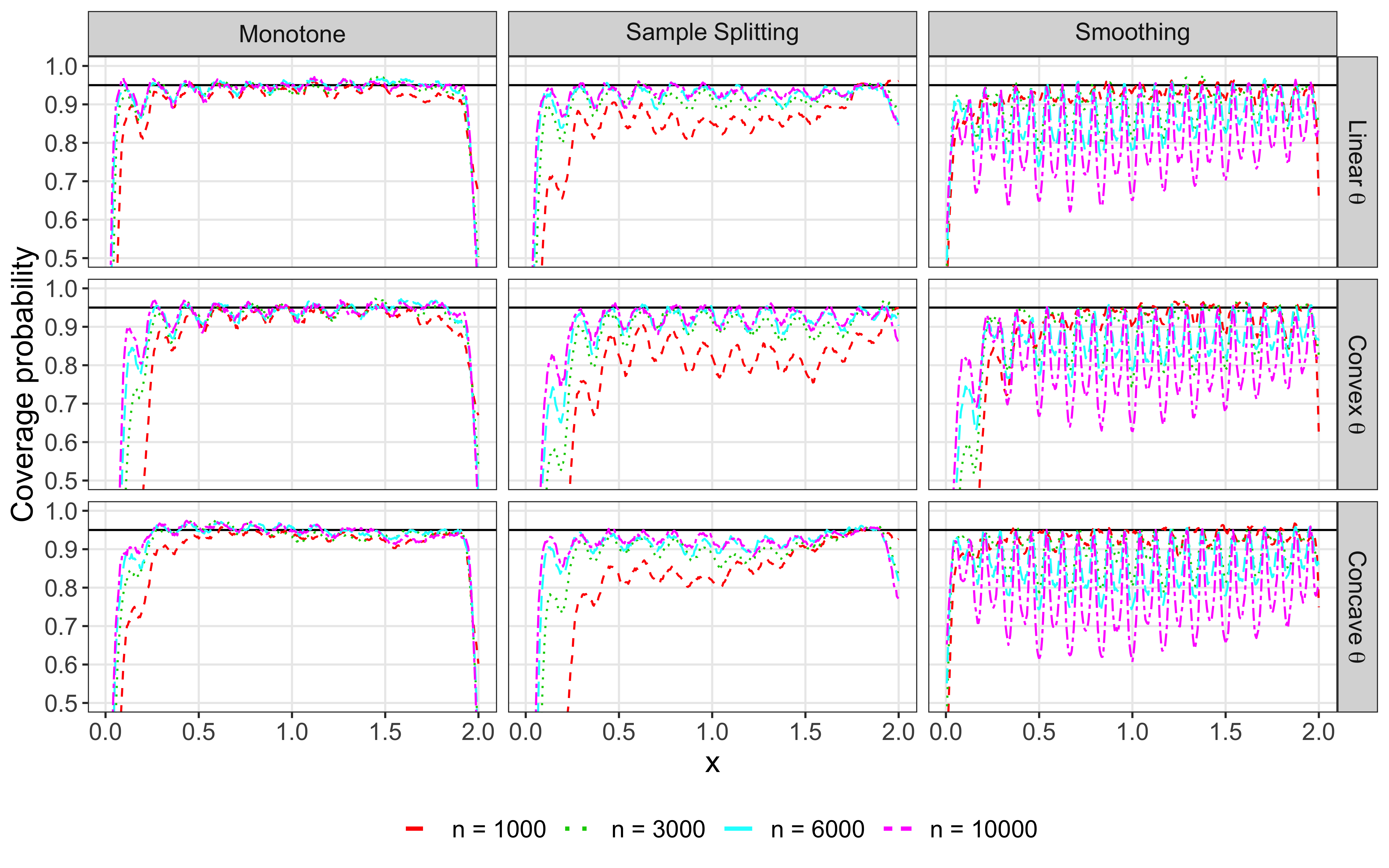
Figure 3 shows the coverage probability of nominal 95% confidence intervals for the three estimators. The coverage of the plug-in intervals centered around our estimator have close to nominal coverage for values of not too close to 0 or 2. For values of close to 0, the coverage of the plug-in method is poor due to the difficulty of estimating the derivative in this region. The sample splitting method has poor coverage for due to high bias, but the coverage converges to the nominal level as the sample size increases. The smoothing-based estimator has poor coverage for values of where the second derivatives of the hazard functions are large, which is due to the bias of the smoothing-based estimator.
5 Analysis of treatment of pulmonary adenocarcinoma
In this section, we use the methods developed in this article to estimate the all-cause mortality hazard ratio of two treatments for pulmonary adenocarcinoma: gefitinib and carboplatin–paclitaxel. Carboplatin-paclitaxel is a type of intravenous chemotherapy, usually taken over a three-hour period once every three weeks for approximately six cycles (Herbst et al. 2004). Like many chemotherapies, carboplatin-paclitaxel is an invasive treatment that can have severe adverse side effects. Gefitinib is a kinase inhibitor that is taken orally as a tablet once per day. Gefitinib is hence less invasive than carboplatin-paclitaxel, but can also cause adverse side effects. We refer the reader to Mok et al. 2009 and Inoue et al. 2013 for additional details about these treatments.
We re-analyzed the results of a clinical trial comparing gefitinib and carboplatin–paclitaxel first reported in Mok et al. 2009. The cohort consisted of adults with stage IIIB or IV non–small-cell lung cancer with histologic features of adenocarcinoma, and who were nonsmokers or former light smokers and had no previous chemotherapy or biologic or immunologic therapy. These patients were randomly assigned to gefitinib (609 patients) or carboplatin–paclitaxel (608 patients). Treatment for both groups continued until progression of the disease, development of unacceptable toxic effects, a request by the patient or physician to discontinue treatment, serious noncompliance with the protocol, or completion of six chemotherapy cycles. The event time of interest was the time from randomization to the earliest sign of disease progression or death from any cause. Additional details of the trial and cohort design can be found in Mok et al. 2009. Since the raw data from this trial are unavailable, we used the event and censoring times reconstructed by Argyropoulos and Unruh 2015 from the published Kaplan-Meier estimates.
Starting from the beginning of treatment, the 12-month estimated survival rates were 24.9% (95% CI: 21.4, 29.4) with gefitinib and 6.7% (95% CI: 4.3, 8.9) with carboplatin–paclitaxel, suggesting that gefitinib was more effective in preventing the progression of pulmonary adenocarcinoma. Mok et al. 2009 also estimated a Cox proportional hazard model with treatment by gefitinib, smoking history and gender and obtained a hazard ratio of 0.74 (95% CI: 0.65, 0.85) corresponding to treatment with gefitinib. They concluded that gefitinib was superior to carboplatin–paclitaxel for treating pulmonary adenocarcinoma.
Although their experimental results confirmed that assignment to gefitinib yielded higher overall 12-month survival probability, the survival curves of the two groups crossed, which suggests that the proportional hazards assumption is violated. Hence, it is of interest to estimate the hazard ratio over time to assess the time-varying effect of gefitinib relative to carboplatin–paclitaxel. The left panel of Figure 4 displays the Nelson-Aalen estimators of the cumulative hazard function for the gefitinib cohort versus that of the carboplation-paclitaxel cohort, and its GCM. This plot suggests that it is reasonable to believe that the hazard ratio function is monotone. Furthermore, prior estimates of the hazard ratio function have also suggested that it is monotone (Argyropoulos and Unruh 2015). Here, we estimate the hazard ratio using our monotone estimator, and construct confidence intervals using the plug-in method described in Section 3.4.

The right panel of Figure 4 displays the estimated hazard ratio of gefitinib versus carboplation-paclitaxel, as well as the constant hazard ratio estimated by the proportional hazard model. The hazard ratio is only shown through month six, since the estimated curve is flat thereafter. We estimate that the hazard ratio increases to one over the span of four months, after which it increases to 1.6 (95% CI: 1.07, 2.10). Hence, we find evidence that the hazard of disease progression for patients assigned to gefitinib is lower than that of patients assigned to carboplation-paclitaxel through four months post-randomization, but is greater after four months. This could be due to a stronger early benefit of gefitinib and a delayed effect of carboplation-paclitaxel. Alternatively, it could be due to heterogeneous effects of carboplation-paclitaxel relative to gefitinib. For example, frailer patients may have been more likely to progress quickly taking carboplation-paclitaxel than taking gefitinib, leaving a less frail cohort with better survival prospects after four months.
Acknowledgements
The authors gratefully acknowledge support from the University of Massachusetts Amherst Department of Mathematics and Statistics startup fund (TW) and NSF Award 2113171 (TW). The authors are also grateful for thoughtful feedback from Anna Liu, John Staudenmayer, and Marco Carone.
References
- Aalen (1978) Aalen, O. (1978). Nonparametric inference for a family of counting processes. The Annals of Statistics, 6(4):701–726.
- Anderson and Senthilselvan (1980) Anderson, J. and Senthilselvan, A. (1980). Smooth estimates for the hazard function. Journal of the Royal Statistical Society: Series B (Methodological), 42(3):322–327.
- Argyropoulos and Unruh (2015) Argyropoulos, C. and Unruh, M. L. (2015). Analysis of time to event outcomes in randomized controlled trials by generalized additive models. PloS ONE, 10(4):e0123784.
- Banerjee et al. (2019) Banerjee, M., Durot, C., Sen, B., et al. (2019). Divide and conquer in nonstandard problems and the super-efficiency phenomenon. Annals of Statistics, 47(2):720–757.
- Banerjee and Wellner (2005) Banerjee, M. and Wellner, J. A. (2005). Confidence intervals for current status data. Scandinavian Journal of Statistics, 32(3):405–424.
- Brunk et al. (1966) Brunk, H., Franck, W., Hanson, D., and Hogg, R. (1966). Maximum likelihood estimation of the distributions of two stochastically ordered random variables. Journal of the American Statistical Association, 61(316):1067–1080.
- Calonico et al. (2018) Calonico, S., Cattaneo, M. D., and Farrell, M. H. (2018). On the effect of bias estimation on coverage accuracy in nonparametric inference. Journal of the American Statistical Association, 113(522):767–779.
- Cox (1972) Cox, D. R. (1972). Regression models and life-tables. Journal of the Royal Statistical Society: Series B (Methodological), 34(2):187–202.
- Deshpande and Sengupta (1995) Deshpande, J. V. and Sengupta, D. (1995). Testing the hypothesis of proportional hazards in two populations. Biometrika, 82(2):251–261.
- Desquilbet and Meyer (2005) Desquilbet, L. and Meyer, L. (2005). Time-dependent covariates in the Cox proportional hazards model. Theory and practice. Revue d’Épidémiologie et de Santé Publique, 53(1):51–68.
- Durham et al. (1998) Durham, L. K., Longini Jr, I. M., Halloran, M. E., Clemens, J. D., Azhar, N., and Rao, M. (1998). Estimation of vaccine efficacy in the presence of waning: application to cholera vaccines. American Journal of Epidemiology, 147(10):948–959.
- Dykstra et al. (1991) Dykstra, R., Kochar, S., and Robertson, T. (1991). Statistical inference for uniform stochastic ordering in several populations. The Annals of Statistics, 19(2):870–888.
- Dykstra et al. (1995) Dykstra, R., Kochar, S., and Robertson, T. (1995). Inference for likelihood ratio ordering in the two-sample problem. Journal of the American Statistical Association, 90(431):1034–1040.
- Dykstra (1982) Dykstra, R. L. (1982). Maximum likelihood estimation of the survival functions of stochastically ordered random variables. Journal of the American Statistical Association, 77(379):621–628.
- Gill and Schumacher (1987) Gill, R. and Schumacher, M. (1987). A simple test of the proportional hazards assumption. Biometrika, 74(2):289–300.
- Groeneboom (1985) Groeneboom, P. (1985). Estimating a monotone density. In Proceedings of the Berkeley Conference in Honor of Jerzy Neyman and Jack Kiefer, 2:539–555.
- Groeneboom et al. (2010) Groeneboom, P., Jongbloed, G., and Witte, B. I. (2010). Maximum smoothed likelihood estimation and smoothed maximum likelihood estimation in the current status model. The Annals of Statistics, 38(1):352 – 387.
- Groeneboom and Wellner (2001) Groeneboom, P. and Wellner, J. A. (2001). Computing Chernoff’s distribution. Journal of Computational and Graphical Statistics, 10(2):388–400.
- Guidoum (2020) Guidoum, A. C. (2020). Kernel estimator and bandwidth selection for density and its derivatives: The kedd package. arXiv: 2012.06102.
- Herbst et al. (2004) Herbst, R. S., Giaccone, G., Schiller, J. H., Natale, R. B., Miller, V., Manegold, C., Scagliotti, G., Rosell, R., Oliff, I., Reeves, J. A., Wolf, M. K., Krebs, A. D., Averbuch, S. D., Ochs, J. S., Grous, J., Fandi, A., and Johnson, D. H. (2004). Gefitinib in combination with paclitaxel and carboplatin in advanced non–small-cell lung cancer: A phase III trial—INTACT 2. Journal of Clinical Oncology, 22(5):785–794.
- Hernán (2010) Hernán, M. A. (2010). The hazards of hazard ratios. Epidemiology, 21(1):13–15.
- Hernandez et al. (2018) Hernandez, I., He, M., Brooks, M. M., and Zhang, Y. (2018). Exposure-response association between concurrent opioid and benzodiazepine use and risk of opioid-related overdose in Medicare Part D beneficiaries. JAMA Network Open, 1(2):e180919.
- Holcomb et al. (2013) Holcomb, J. B., Del Junco, D. J., Fox, E. E., Wade, C. E., Cohen, M. J., Schreiber, M. A., Alarcon, L. H., Bai, Y., Brasel, K. J., Bulger, E. M., et al. (2013). The prospective, observational, multicenter, major trauma transfusion (PROMMTT) study: comparative effectiveness of a time-varying treatment with competing risks. JAMA Surgery, 148(2):127–136.
- Huang and Wellner (1995) Huang, J. and Wellner, J. A. (1995). Estimation of a monotone density or monotone hazard under random censoring. Scandinavian Journal of Statistics, 22:3–33.
- Inoue et al. (2013) Inoue, A., Kobayashi, K., Maemondo, M., Sugawara, S., Oizumi, S., Isobe, H., Gemma, A., Harada, M., Yoshizawa, H., Kinoshita, I., et al. (2013). Updated overall survival results from a randomized phase III trial comparing gefitinib with carboplatin–paclitaxel for chemo-naïve non-small cell lung cancer with sensitive EGFR gene mutations (NEJ002). Annals of Oncology, 24(1):54–59.
- Kalbfleisch and Prentice (2011) Kalbfleisch, J. D. and Prentice, R. L. (2011). The Statistical Analysis of Failure Time Data. John Wiley & Sons.
- Kaplan and Meier (1958) Kaplan, E. L. and Meier, P. (1958). Nonparametric estimation from incomplete observations. Journal of the American Statistical Association, 53(282):457–481.
- Kim et al. (2017) Kim, G., Kim, Y., and Choi, T. (2017). Bayesian analysis of the proportional hazards model with time-varying coefficients. Scandinavian Journal of Statistics, 44(2):524–544.
- Kim et al. (2011) Kim, Y., Park, J. K., and Kim, G. (2011). Bayesian analysis for monotone hazard ratio. Lifetime Data Analysis, 17(2):302–320.
- Klein and Moeschberger (2003) Klein, J. P. and Moeschberger, M. L. (2003). Survival Analysis: Techniques for Censored and Truncated Data. Springer.
- Lehmann and Rojo (1992) Lehmann, E. L. and Rojo, J. (1992). Invariant directional orderings. The Annals of Statistics, 20(4):2100–2110.
- Li et al. (2015) Li, H., Han, D., Hou, Y., Chen, H., and Chen, Z. (2015). Statistical inference methods for two crossing survival curves: a comparison of methods. PLoS ONE, 10(1):e0116774.
- Mok et al. (2009) Mok, T. S., Wu, Y.-L., Thongprasert, S., Yang, C.-H., Chu, D.-T., Saijo, N., Sunpaweravong, P., Han, B., Margono, B., Ichinose, Y., et al. (2009). Gefitinib or carboplatin–paclitaxel in pulmonary adenocarcinoma. New England Journal of Medicine, 361(10):947–957.
- Müller and Wang (1990) Müller, H.-G. and Wang, J.-L. (1990). Locally adaptive hazard smoothing. Probability Theory and Related Fields, 85(4):523–538.
- Müller and Wang (1994) Müller, H.-G. and Wang, J. L. (1994). Hazard rate estimation under random censoring with varying kernels and bandwidths. Biometrics, 50 1:61–76.
- Mösching and Dümbgen (2020) Mösching, A. and Dümbgen, L. (2020). Estimation of a likelihood ratio ordered family of distributions – with a connection to total positivity. arXiv:2007.11521.
- Nelson (1969) Nelson, W. (1969). Hazard plotting for incomplete failure data. Journal of Quality Technology, 1(1):27–52.
- O’Quigley (2008) O’Quigley, J. (2008). Proportional Hazards Regression. Springer.
- Præstgaard and Huang (1996) Præstgaard, J. T. and Huang, J. (1996). Asymptotic theory for nonparametric estimation of survival curves under order restrictions. The Annals of Statistics, 24(4):1679–1716.
- R Core Team (2021) R Core Team (2021). R: A Language and Environment for Statistical Computing. R Foundation for Statistical Computing, Vienna, Austria.
- Rebora et al. (2014) Rebora, P., Salim, A., and Reilly, M. (2014). bshazard: A flexible tool for nonparametric smoothing of the hazard function. The R Journal, 6(2):114–122.
- Sekula et al. (2013) Sekula, P., Dunant, A., Mockenhaupt, M., Naldi, L., Bavinck, J. N. B., Halevy, S., Kardaun, S., Sidoroff, A., Liss, Y., Schumacher, M., et al. (2013). Comprehensive survival analysis of a cohort of patients with Stevens–Johnson syndrome and toxic epidermal necrolysis. Journal of Investigative Dermatology, 133(5):1197–1204.
- Shaked and Shanthikumar (2007) Shaked, M. and Shanthikumar, J. G. (2007). Stochastic Orders. Springer Science & Business Media.
- Strimmer (2008) Strimmer, K. (2008). fdrtool: a versatile R package for estimating local and tail area-based false discovery rates. Bioinformatics (Oxford, England), 24(12):1461–1462.
- Struthers and Kalbfleisch (1986) Struthers, C. A. and Kalbfleisch, J. D. (1986). Misspecified proportional hazard models. Biometrika, 73(2):363–369.
- Stute (1994) Stute, W. (1994). Strong and weak representations of cumulative hazard function and Kaplan-Meier estimators on increasing sets. Journal of Statistical Planning and Inference, 42(3):315–329.
- Therneau (2022) Therneau, T. M. (2022). A Package for Survival Analysis in R. R package version 3.3-1.
- van der Vaart and van der Laan (2006) van der Vaart, A. and van der Laan, M. J. (2006). Estimating a survival distribution with current status data and high-dimensional covariates. The International Journal of Biostatistics, 2(1):
- van der Vaart (2000) van der Vaart, A. W. (2000). Asymptotic Statistics. Cambridge University Press.
- van der Vaart and Wellner (1996) van der Vaart, A. W. and Wellner, J. A. (1996). Weak Convergence and Empirical Processes. Springer.
- Wasserman (2013) Wasserman, L. (2013). All of Statistics: A Concise Course in Statistical Inference. Springer Science & Business Media.
- Watson and Leadbetter (1964) Watson, G. and Leadbetter, M. (1964). Hazard analysis. I. Biometrika, 51(1/2):175–184.
- Westling et al. (2020a) Westling, T., Carone, M., et al. (2020a). A unified study of nonparametric inference for monotone functions. Annals of Statistics, 48(2):1001–1024.
- Westling et al. (2021) Westling, T., Downes, K. J., and Small, D. S. (2021). Nonparametric maximum likelihood estimation under a likelihood ratio order. Statistica Sinica, page Advance online publication.
- Westling et al. (2020b) Westling, T., van der Laan, M. J., and Carone, M. (2020b). Correcting an estimator of a multivariate monotone function with isotonic regression. Electronic Journal of Statistics, 14(2):3032–3069.
- Whitney et al. (2019) Whitney, D., Shojaie, A., and Carone, M. (2019). Comment: Models as (deliberate) approximations. Statistical Science: A Review Journal of the Institute of Mathematical Statistics, 34(4):591–598.
- Yu et al. (2017) Yu, T., Li, P., and Qin, J. (2017). Density estimation in the two-sample problem with likelihood ratio ordering. Biometrika, 104(1):141–152.
Supplementary Material
Supplementary figures


Proof of Theorems
Proof of Theorem 1.
(1) For any , we can take , so that on the support of , and . We then have on the support of , which is monotone.
(2) Suppose and . Let , , and . We can take to be a measure dominating , , and . We want to show that for all such that . Let be such that . Then since and , . Similarly, since and , . Hence,
We now need to address
If , then , which is guaranteed to be no larger than . Similarly, if , then , which is guaranteed to be no smaller than .
The only remaining case is and . We show there cannot simultaneously be such with . First, if , then , which implies since that for all with . This implies that for all such , so that is not in . Therefore, for all . Similarly, if , then , which implies since that for all with . This implies that for all such , so that is not in . Therefore, for all . Since cannot be empty, this completes the proof of (2).
(3) If and are both dominated by , then and are both dominated by . Let be the density of with respect to , and be the density of with respect to . Then , so
Since and are monotone, so is . ∎
Lemma 1.
Suppose that is an interval and that is a non-decreasing and càdlàg function, and is continuous on . Let . Then is non-decreasing on if and only if is convex on , and if is non-decreasing on then for all , where is the smallest interval in containing .
Proof of Lemma 1.
We first show that if is non-decreasing on , then is convex on . Suppose we have , where and . Defining , we have
Now, for any , . Thus, by plugging into the above inequality, we have , which implies that . Therefore, is convex on .
Next, we show that if is continuous on , and is convex on , then is non-decreasing on . The idea is to compare the slopes of chords of using the convexity of . Let be such that . Suppose there exist two sequences and such that and , where
If for all large enough, then convexity of on would imply that for all large enough, and hence . Hence, if we can find such sequences, we have established the claim. The slopes of the chords of depend on the behavior of near and , each of which has three cases. We note that since by assumption, exactly one of the following three situations must hold: (y1) and there exists such that , (y2) but there’s no such that , and (y3) . There are three analogous cases for : (x1) and there exists such that , (x2) but there’s no such , and (x3) . We proceed by defining and in each case.
In case (y1), we let for all . We can set and still have . We know that ; if then is in by assumption, and if , then for all since , in which case as well. Hence, necessarily. We therefore have
since is by assumption flat on and has a jump at .
In case (y2), we have . Thus, there exists increasing to such that for each and increases to . Therefore, converges to . Hence converges to since possesses left-limits, showing that converges to . In case (y3), since , there exists that either (y3a) increases to and for each , or (y3b) decreases to and for each . In case (y3a), since for all , we have
By continuity of over , for any , we can find such that implies for all . We then have
for all , so . If (y3b) holds, then a similar argument shows that . Applying the same exact reasoning for the three cases for , we see that converges to .
We have now shown that there exist sequences and such that converges to and converges to , where and are defined above. Hence, if for all large enough, then convexity of on implies that for all large enough, and hence . It is clear that for all 16 pairings of definitions of and implied by cases (x1)–(x3b) and (y1)–(y3b) except for when decreases to (case x3b) and (case y1). In this case, we note that if , then is flat on , so that case (x3b) cannot hold. Therefore, if decreases to and , then must be strictly larger than , so that for all large enough.
Next we prove the second claim of the lemma: if is continuous and non-decreasing on , then for all , where is the smallest interval containing . We have proved that is convex on under the stated conditions. First, we claim that , where has the following form. For any . If but , then there exists and such that . We then define . Thus defined, is the linear interpolation of to all of . In order to show that , we need to show that (a) is convex, (b) and (c) for any other convex minorant of .
For (a), let and for . Since is the smallest interval containing , there exist that are all elements of and such that , , and , and such that , and . (If , then we set and . Otherwise, we can find with and in exist since is the smallest interval containing , and such a exists by the definition of . We define similarly, and we can ensure that the stated ordering is satisfied since .)
We define the points . The convexity of implies that the (possibly degenerate) line segment lies on or below , which lies on or below , which lies on or below . Since lies on and the point lies on the line , we have . Since , and were arbitrary, this implies that is convex.
For (b), if , by definition . If , then since for some , we must have . Consequently, by the convexity and continuity of on
For (c), if is another convex minorant of , then for all . If , we have for some . By convexity of on and since by assumption,
If , then since is continuous on , so the above equals
If , then for all there exists such that , since otherwise would be flat to the left of and would be in . We then have , where and as . Taking the limit of , we have .
Finally, we show that for all . If , then for all and , we have
Thus . If , then and it’s clear that . ∎
Proof of Theorem 2.
We note that since and . In addition, . Therefore, we can write . Hence, (1) (3) and (b) follow by Lemma 1 with , , and .
It remains to show (1) (2). By Lemma 1 with , and , is nondecreasing on if and only if
is convex on . Hence, if
then (1) (2). We can write
for the continuous part of . We address the discrete and continuous parts of the integral in turn.
We note that if and only if , which implies that , since otherwise . Furthermore if and only if is flat on , which implies is too. But if then , which implies , and therefore as well, have jumps at . Hence, if and only if and are both flat on and have a jump at , and and . Therefore, for any with ,
Therefore,
where the last equality follows because if and only if .
We now address the continuous part of the integral. Using the fact derived above that for any with , we have
Therefore,
We then note that implies that , and hence unless is at the left end of a flat of . Such points form a measure zero set. Similarly, if , then , and such that form a measure zero set. Therefore, we have
Now we note that is strictly increasing on the support of , so by the change of variables , we have
Now except on a -measure zero set, , , and . Therefore,
Finally, we note that if , then is flat on , and if and only if , so
Putting together the discrete and continuous parts of the integral, we now have
∎
We denote as the empirical distribution of , as the true distribution of (as implied by , , , , and ), and . For any probability distribution and -integrable function , we denote . We also let be the observed fraction of treated units.
Proof of Theorem 3.
To prove Theorem 3, we will use Theorem 4 of Westling et al. 2020a. For convenience, we refer to Westling et al. 2020a as WC hereafter. In the notation of WC, we have , , , and . To use Theorem 4 of WC, we need to first verify that the decomposition of equation (2) of WC holds, and then verify conditions (B1) – (B5) and (A4) – (A5) of WC. We establish each of these in turn below.
Equation (2) of WC. We define the influence function and of and as
By adding and subtracting terms, we have and , where
These are the functions corresponding to equation (2) of WC.
Condition (B1). We define the local difference function
To verify condition (B1), we need to bound the uniform entropy of the class for all small enough. We further decompose for and . The function can be written as
The class of functions is Vapnik-C̆ervonenkis (VC) with index 2 (see, e.g. Lemma 2.6.16 of van der Vaart and Wellner 1996). The class
is a Lipschitz transformation of and various fixed square-integrable functions, so it is also VC, and hence easily satisfies condition (B1b) of WC. In conjunction with Lemma 5.2 of van der Vaart and van der Laan 2006, this also implies that the class
is VC. Hence, satisfies (B1b). By the analogous forms of and , an identical argument shows that satisfies (B1b), so does as well.
Condition (B2). An envelope function for is given by for
We now verify that as under the stated conditions. Due to the boundedness of and away from zero and independent censoring,
for some . This latter expression is as because is continuously differentiable at with finite derivative.
Next, by Jensen’s inequality,
As above, the last expression is as because is Lipschitz at and and are both positive in a neighborhood of . By the triangle inequality, we then have .
For the second part of condition (B2), we note that since and are both positive in a neighborhood of , is uniformly bounded for all small enough. Hence, for all , for all small enough (possibly depending on ), is identically 0, which implies in particular that . Identical analysis applies to an envelope for .
Condition (B3). This condition concerns properties of the covariance function defined as . Since for , for any . Hence, . We write
| (1) |
We will address each term in this expansion. We first have
Next, the second term can be simplified as follows
Similarly, the third term can be written as
Finally, for the last term, by decomposing the double integral into two regions, we can write
Hence, the second through fourth terms in the decomposition of provided in equation (1) cancel, and we are left with
By symmetry of and , we also have
Thus, we can write
In the notation of condition (B3) of WC, we have ,
, and can be taken as any probability measure since there are no covariates.
Sub-conditions (B3a) and (B3d) are automatically satisfied. Sub-condition (B3b) is satisfied because does not depend on or . Sub-condition (B3c) requires that be continuous at , which would appear to require that and are continuous at . However, in the proof of Theorem 4 on pages 4 and 5 of the Supplementary Material of WC, it is actually only used that possesses a right-limit as approaches from above (since in the proof stands in for , which is positive), in which case should take the place of in the result. This is important in our work because in many applications the censoring distributions and possess mass points. Hence, this weaker version of sub-condition (B3c) holds with
Thus, condition (B3) holds, and the scale parameter is
Conditions (B4) and (B5). For these two conditions, we define , and . For (B4), we need to show that for each , and for (B5), we need to show that for some , is decreasing for all large enough and small enough. As above, we only verify the conditions for , since verification for is completely analogous.
We define
Then by the definition of the Nelson-Aalen estimator and the definition of the cumulative hazard function with independent right censoring, we can write
We let and . We note that and that and are bounded away from zero in a neighborhood of almost surely for all large enough. Hence, there is a constant C such that almost surely for all large enough and small enough,
We address each term in turn. For any fixed and , we define the function class . The class is uniformly bounded by 1 and -Donsker for any . Since and , we can then write
Therefore, we also have
Next, since and are non-decreasing functions, we have
Using a similar approach as for , we can show that
Turning to , since and is continuously differentiable in a neighborhood of , we have
We conclude that . Finally, since , we have . Putting it together, we have
This goes to zero for each , which verifies (B4), and (B5) is satisfied for any .
Condition (A4). For condition (A4), it suffices to show that for some . We define , , , and as we did above for , but with in the conditionals instead. We then have
We used integration by parts to bound the first term in the second inequality. By assumption, is bounded away from zero in a neighborhood of , and as a result, is almost surely bounded away from zero in a neighborhood of for all large enough. Then, for some and , almost surely for all large enough it holds that
We can show that this expression is using similar empirical process techniques as we did with above.
Condition (A5). For this condition, since , it suffices to show that the stratified Nelson-Aalen estimators are uniformly consistent on , i.e. and tend to zero in probability. This follows from Corollary 1.2 of Stute 1994 by the assumed lower bound for . ∎