Many-Fermion Simulation from the Contracted Quantum Eigensolver without Fermionic Encoding of the Wave Function
Abstract
Quantum computers potentially have an exponential advantage over classical computers for the quantum simulation of many-fermion quantum systems. Nonetheless, fermions are more expensive to simulate than bosons due to the fermionic encoding—a mapping by which the qubits are encoded with fermion statistics. Here we generalize the contracted quantum eigensolver (CQE) to avoid fermionic encoding of the wave function. In contrast to the variational quantum eigensolver, the CQE solves for a many-fermion stationary state by minimizing the contraction (projection) of the Schrödinger equation onto two fermions. We avoid fermionic encoding of the wave function by contracting the Schrödinger equation onto an unencoded pair of particles. Solution of the resulting contracted equation by a series of unencoded two-body exponential transformations generates an unencoded wave function from which the energy and two-fermion reduced density matrix (2-RDM) can be computed. We apply the unencoded and the encoded CQE algorithms to the hydrogen fluoride molecule, the dissociation of oxygen O2, and a series of hydrogen chains. Both algorithms show comparable convergence towards the exact ground-state energies and 2-RDMs, but the unencoded algorithm has computational advantages in terms of state preparation and tomography.
I Introduction
Simulations on quantum computers have a potentially exponential advantage for the computation of many-fermion quantum systems such as molecules and materials Abrams and Lloyd 1997; Whitfield et al. 2011. However, if each qubit represents the particle filling of an orbital, as in the formalism of second quantization, the natural particles for simulation on a quantum computer—qubit particles—are hard-core bosons rather than fermions Mazziotti et al. 2021; Wu and Lidar 2002. Consequently, as originally recognized by Feynman Feynman 1982, the simulation of a many-fermion quantum system is potentially more complicated than the simulation of an equivalent many-boson quantum system. The particle statistics of fermions are typically encoded in the qubit wave function in a process known as fermionic encoding, which increases computational complexity in terms of the quantum state preparation and tomography Jordan and Wigner 1928; Abrams and Lloyd 1997; Bravyi and Kitaev 2002; Seeley et al. 2012; Hastings et al. 2014; Wecker et al. 2014.
To avoid this additional complexity, hardware-efficient wave functions have been developed for fermionic systems in which a wave function is prepared on the quantum computer such that its simulated particles are neither bosons nor fermions Kandala et al. 2017; Choquette et al. 2020; Barron et al. 2020. Encoding the Hamiltonian with fermion statistics in these instances still recovers the many-fermion energy from the arbitrary statistics of the prepared wave function. While the absence of particle statistics can produce optimization difficulties such as barren plateaus, more accurate results have recently been obtained by using qubit-particle wave functions whose particles have the statistics of hard-core bosons Xia and Kais 2020; Izmaylov et al. 2020; Ryabinkin et al. 2018; Ryabinkin et al. 2020; Ryabinkin et al. 2021; Tang et al. 2021. We have shown that, in contrast to the hardware-efficient wave functions, the qubit-particle wave functions are isomorphic to the fermion wave functions, and hence, they uniquely parameterize the set of ground-state two-fermion reduced density matrices (2-RDMs) Mazziotti et al. 2021. Consequently, the energy and 2-RDM of a many-fermion quantum system can be computed from a qubit-particle wave function with the accuracy associated with a fermion wave function but at a potentially reduced computational cost.
Recently, we presented a hybrid quantum-classical algorithm for the many-fermion problem known as the contracted quantum eigensolver (CQE) Smart and Mazziotti 2021a; Boyn et al. 2021; Smart et al. 2022. The CQE minimizes the residual of a contraction (projection) of the Schrödinger equation onto the space of two particles. The algorithm updates the fermion wave function iteratively with two-body exponential transformations to minimize the residual. To keep the transformations unitary, we use the anti-Hermitian part of the contraction of the Schrödinger equation, known as the anti-Hermitian contracted Schrödinger equation (ACSE) Mazziotti 2006; Mazziotti 2007a; Mazziotti 2007b; Gidofalvi and Mazziotti 2007; Rothman et al. 2009; Snyder and Mazziotti 2012; Sand and Mazziotti 2015; Boyn and Mazziotti 2021. In contrast to the variational quantum eigensolver (VQE) Peruzzo et al. 2014; McClean et al. 2016; Romero et al. 2019 in which the variational form of the wave function is not specified, the CQE produces a compact wave function Ansatz consisting of a series of two-body exponential transformations applied to the reference wave function. This CQE Ansatz Mazziotti 2007a, which is significantly more flexible than a truncated coupled cluster Ansatz, can be converged to the exact solution of the Schrödinger equation. The CQE algorithm, which stores just the 2-RDM on the classical computer, has a potentially exponential advantage over classical methods for solving the -fermion problem like full configuration interaction.
Here we develop a generalization of the CQE algorithm for the many-fermion problem that solves an unencoded ACSE in which the anti-Hermitian part of the Schrödinger equation is contracted onto two qubit particles rather than two fermions. The generalized algorithm solves for the fermionic ground-state energy and 2-RDM by updating a qubit-particle wave function at each iteration with a two-qubit-particle unitary transformation that minimizes the residual of the unencoded ACSE. We explore the accuracy and efficiency of the proposed algorithm through quantum simulations of the hydrogen fluoride molecule, the dissociation of diatomic oxygen O2, and a series of hydrogen chains. Both the encoded (fermion) and the unencoded (qubit-particle) CQE algorithms show similar convergence to the exact ground-state energies and 2-RDMs, but the unencoded CQE has potentially important computational savings in terms of the number of two-qubit gates required in the state preparation and the locality of the 2-RDM tomography.
II Theory
We review the ACSE and its CQE algorithm for quantum simulation in section II.1, present the unencoded ACSE and its CQE algorithm that avoid fermionic encoding of the wave function in section II.2, explore the connection between the encoded and unencoded ACSEs in section II.4, and discuss practical considerations for both encoded and unencoded CQE algorithm in section II.5.
II.1 Encoded ACSE and its CQE algorithm
Consider a fermionic quantum system of fermions in orbitals described by the Schrödinger equation
| (1) |
Here and are the many-fermion ground-state energy and wave function, and is the Hamiltonian operator
| (2) |
in which is the reduced Hamiltonian matrix, the indices ranging from one to denote the orbitals, and and are the creation and annihilation operators of the fermion in the orbital. The ACSE is the anti-Hermitian contraction of the many-fermion Schrödinger equation onto two fermions Mazziotti 2006; Mazziotti 2007a; Mazziotti 2007b; Gidofalvi and Mazziotti 2007; Rothman et al. 2009; Snyder and Mazziotti 2012; Sand and Mazziotti 2015; Boyn and Mazziotti 2021:
| (3) |
As shown in previous work, iterative solution of the ACSE generates a unitary two-body exponential Ansatz for the wave function Mazziotti 2007a; Smart and Mazziotti 2021a
| (4) |
in which is the reference wave function and the unitary transformation at the iteration is determined by a two-body anti-Hermitian operator
| (5) |
that corresponds to the residual of the ACSE
| (6) |
The residual the ACSE at the iteration equals the gradient of the energy with respect to the two-body anti-Hermitian operator . Hence, the residual the ACSE is zero not only when the ACSE is satisfied but also when the gradient of the energy vanishes. The is a step-like parameter that can be optimized at the iteration to minimize the energy. From the wave function the elements of the 2-RDM at the iteration can be computed
| (7) |
While calculation of the residual the ACSE and the 2-RDM on the classical computer typically requires a cumulant approximation for the three-particle reduced density matrix (3-RDM) Mazziotti 1998a; Mazziotti 1998b to avoid storage of the wave function, both the ACSE residual and the 2-RDM in the CQE algorithm can be directly calculated by quantum tomography. Implementation of the state preparation and tomography in the CQE requires fermionic encoding in which the fermionic creation and annihilation operators are expressed in terms of qubit operators through a transformation such as the Jordan-Wigner mapping.
II.2 Unencoded ACSE and its CQE algorithm
In this paper we generalize the CQE algorithm to solve the many-fermion problem using a qubit-particle wave function that does not require fermionic encoding. Consider the anti-Hermitian contraction of the Schrödinger equation onto two qubit particles to generate the unencoded ACSE
| (8) |
where the Hamiltonian is defined with fermionic operators as in Eq. (1) but the and are the creation and annihilation operators of a qubit particle in the orbital. As in the previous case of the contraction onto two fermions to generate the ACSE (or encoded ACSE), iterative solution of the unencoded ACSE generates a unitary two-qubit-particle exponential Ansatz for the wave function
| (9) |
in which the unitary transformation at the iteration is determined by a two-qubit-particle anti-Hermitian operator
| (10) |
that corresponds to the residual of the unencoded ACSE
| (11) |
The residual of the unencoded ACSE at the iteration equals the gradient of the energy with respect to the two-qubit-particle anti-Hermitian operator. Computation of the 2-RDM uses the definition in Eq. (7). Importantly, the CQE algorithm for solving the unencoded ACSE does not require fermionic encoding in the preparation of the wave function since the exponential Ansatz in Eq. (9) is expressed entirely in terms of qubit-particle creation and annihilation operators. Only the definitions of the 2-RDM and the Hamiltonian use fermionic second-quantized operators that require fermionic encoding into qubits for evaluation on quantum computers. A schematic of the CQE algorithm is shown in Fig. 1.
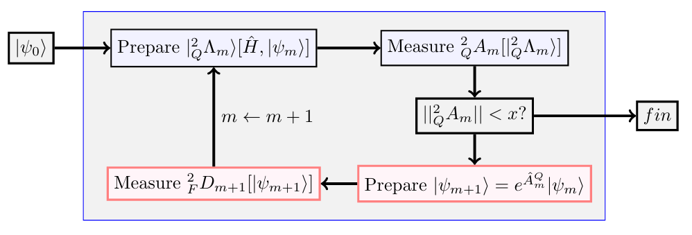
Following previous work Smart and Mazziotti 2021a, we can compute the residual of the ACSE through an auxiliary state
| (12) |
such that
| (13) |
where is the imaginary component of and is a short time-like step, which for stochastic simulations should be larger than the sampling error. If the RDM solutions are complex, we can evaluate the residual by a centered finite difference using two auxiliary states at Smart and Mazziotti 2021a. The approximation from a finite can potentially be minimized by using extrapolative techniques as in the unitary decomposition of operators Schlimgen et al. 2021. As discussed in the Appendix, the evaluation of the residual via the auxiliary state can be implemented efficiently in terms of the two-qubit gate count through first-order or Cholesky factorizations of the Hamiltonian. For completeness we also note that it is possible to compute the residual without defining an auxiliary state but that the required tomography involves the measurement of a 4-particle RDM.
II.3 Second-order Corrections to the Wave Functions and 2-RDMs
Solution of either the encoded or unencoded ACSE can be accelerated through a second-order correction at each iteration. We have the following generalized exponential expansions
| (14) |
and
| (15) |
in which
| (16) |
and
| (17) |
where either or are modifications to the gradient direction and can be equal to (i) zero to recover the first-order Ansatz or (ii) a second-order correction such as that from a quasi-Newton method Nocedal and Wright 2006. In general, a quasi-second-order correction accelerates convergence of the CQE, the implementation and further development of which is explored in concurrent work Smart and Mazziotti 2022a.
II.4 Connection between the Encoded and Unencoded ACSEs
Before we consider the relationship of the solutions to the encoded ACSE, or just ACSE, and the unencoded ACSE, we examine the relationship between the solution of the ACSE and the solution of the many-fermion Schrödinger equation. Consider the contracted Schrödinger equation (CSE) Mazziotti 1998a; Mazziotti 2007c; Nakatsuji 1976
| (18) |
If we expand the wave function in terms the eigenfunctions of the Hamiltonian
| (19) |
we can formally write the CSE as
| (20) |
Because the CSE is equivalent to the energy variance which implies the Schrödinger equation, the CSE is satisfied by an -fermion wave function if and only if the Schrödinger equation is satisfied Mazziotti 1998a; Mazziotti 2007c; Nakatsuji 1976. Hence, the CSE is zero for the ground state if and only if the expansion coefficients of excited states () vanish. Substitution of the wave function expansion into the ACSE in Eq. (3) yields the expression
| (21) |
As with the CSE, the ACSE is zero if the expansion coefficients of excited states () vanish. This condition also implies the CSE as well as the Schrödinger equation. In contrast to the CSE, however, the ACSE does not strictly imply the Schrödinger equation Mazziotti 2007a. It is theoretically possible for the ACSE to vanish due to a cancellation of the anti-Hermitian terms, which in the expansion are represented by the energy differences . Practical calculations, however, indicate that such cancellations do not occur easily and that the ACSE can in principle be converged to exact ground-state energies and 2-RDMs, especially with quasi-second-order corrections.
To understand the relationship between the solutions of the ACSE and unencoded ACSE, we express the residuals of both equations in terms of two parts
| (22) |
and
| (23) |
where the plus (minus) indicates the contributions from the wave function to the expectation value with net even (odd) permutations of particles. Because the fermion and qubit-particle expectation values differ only from the sign of the odd permutations, we have the following two important relations
| (24) | |||||
| (25) |
Substituting these relations into the residual of the unencoded ACSE yields the following equation
| (26) |
Comparing this equation for the qubit-particle residual with the fermion residual in Eq. (22), we observe that the only difference in the two residuals is the sign change of the second term. If both the plus and minus terms converge to zero, then both the ACSE and unencoded ACSE produce identical solutions. While it is in principle possible for the plus and minus terms to produce a spurious solution through an exact cancellation, because the Schrödinger equation implies both the ACSE and the unencoded ACSE, both the positive and negative terms will tend to zero as the energy is minimized towards a stationary state by either encoded or unencoded unitary transformations. The relative magnitudes of the residuals and are related to the relative rates of convergence of the ACSE and the unencoded ACSE. A larger residual norm indicates less cancellation of the plus and minus terms which is likely to result in a faster rate of convergence towards the solution of the Schrödinger equation.
II.5 Practical Considerations of the CQE Algorithm
Finally, we introduce two practical aspects of the CQE , applicable to both encoded and unencoded variants, that are important for its implementation on a quantum computer. We discuss: (i) a sparsification of the operators in which at each iteration matrix elements below a given threshold are set to zero, and (ii) an approximate combination of operators for in which parts of the set of operators are combined to decrease the circuit length. Given the matrix elements of the residual of the encoded or unencoded ACSE in Eqs. (6) or (11), respectively, we define a sparsification operation that zeros matrix elements below a given threshold
| (27) |
where the scalar factor and the infinity norm of is the element with the largest absolute value. When , is equivalent to the identity mapping, and when , is equivalent to selecting only the highest amplitude element. Given a choice of the parameter , we use this mapping at each iteration of the CQE to prune the residual matrix . Formally, at each iteration is replaced by .
After defining a sparser matrix in , we still need to express the operator as a product of unitary transformations, which is traditionally performed by trotterization. We choose a first-order trotterization which is valid in the case that is not too large. Moreover, because the algorithm is greedy by design with the gradient being used at each iteration, the algorithm has the ability to adjust itself in part to errors in previous iterations including those from trotterization.
To address the growth of the circuit length with iterations, we define an approximate combination of operators for , which we call the -depth. When updating the wave function at the iteration, we examine the elements of that were not pruned in one of the previous steps. If for an in is non-zero, we update that term as follows:
| (28) |
In this manner we collect terms to decrease circuit length even if the collection is approximate. Importantly, the computed residual of the ACSE at the next iteration adjusts for errors introduced in previous terms in the product expansion of the wave function. Other works exploit a classification of the commutating operators in the Hamiltonian or the unitary transformation of the wave function to minimize the circuit length, and these schemes can also be applied to the CQE algorithm.
The -depth and techniques are closely related, and in their extreme limits they produce specific Ansätze. For , a large is reasonable, because each iteration will contain only one or a few terms, and hence, setting or will not simplify the product of terms. On the other hand, when , setting or may be necessary because a larger may generate a single exponential Ansatz, which negates a critical benefit of the CQE—the ACSE Ansatz for the wave function.
III Applications
III.1 Molecular Simulations
We compare the encoded and unencoded CQE for several molecular systems, H4, H5, H6, as well as hydrogen fluoride, at equilibrium geometries in the minimal Slater-type orbital basis (STO-3G) set Hehre, W. J.; Ditchfield, R.; Pople 1972. The convergence of the two CQE algorithms is shown in Fig. 2. For H6 we select in the truncation, whereas for the other cases . In all cases the encoded and unencoded algorithms show convergence towards the solution of the Schrödinger equation in the given basis set even without any second-order acceleration of the transformations at each iteration. In some instances, the two algorithms can exhibit nearly identical convergence, especially in systems with significant pairing of the orbitals, as in an antisymmetrized geminal power wave function Coleman 1997; Coleman and Yukalov 2000; Johnson et al. 2013; Stein et al. 2014, where the particle statistics become less important Sager and Mazziotti 2022. One such example is hydrogen fluoride whose hole wave function in the minimal basis set is a single two-hole function or a geminal. The molecule H5 exhibits greater differences between the fermionic and qubit-particle Ansätze, which is expected for open-shell or strongly correlated molecules.

To examine performance for non-equilibrium geometries, we apply the encoded and unencoded CQE to computing the potential energy curves of H4 and O2. We use approximate second-order transformations, based on a quasi-Newton method, as each iteration to accelerate convergence. Figure 2 shows the obtained energies across the dissociation curve. For a convergence criteria of 0.001 in the ACSE’s residual norm, we consistently obtain high accuracy results at both equilibrium and non-equilibrium geometries regardless of the encoding.

III.2 Investigation of Resource Requirements
We examine the resource requirements for the encoded and unencoded methods. Two cases, equilibrium and stretched geometries of linear H4, are considered. We examine the necessary resources to converge the residual of the ACSE within 0.01 as a function of the -depth and the sparse parameter with results in Table 1.
First, in the equilibrium case (top half), for , neither the fermionic nor the qubit-particle Ansatz changes with depth but each requires more iterations than when or . In all of the instances, the qubit-particle wave function matches the fermionic wave function’s trends but has 703% of the fermionic CNOT cost. Additionally, the -depth leads to a significant reduction in the number of terms. Including the previous iteration () results in 55% of the count for , and 66% of the count for (equivalent circuits for ). The case shows even further reductions, requiring about 13% and 34% of the cost for the and cases, respectively. We can reasonably infer that the -depth and sparse of the operator can greatly impact the CQE’s resource requirements as well as its rate of convergence.
For the stretched geometries the savings are more difficult to analyze. For again we have a similar picture across -depths, with notably more iterations required than for the equilibrium case. Again, the qubit case appears to have a similar advantage in the CNOT gate reduction versus the fermionic case. For other truncations, we lose the correspondence between the qubit-particle and fermionic wave functions. For multiple cases (i.e., when ), the qubit case requires either more iterations or yields a higher CNOT gate count. However, the shortest apparent Ansatz is still the qubit case. The difference in the -depth plays a more significant role, which leads to almost a 100-fold decrease in CNOT requirements between and for , as well as a similar trend for .
| depth | Average | ||||
| 1568 [9] | 6782 [9] | 12494 [9] | |||
| 2020 [8] | 3858 [8] | 6068 [8] | |||
| 1263 [16] | 1408 [16] | 1408 [16] | |||
| 1162 [9] | 4974 [9] | 9014 [9] | |||
| 1414 [8] | 2756 [8] | 4098 [8] | |||
| 840 [16] | 928 [16] | 928 [16] | |||
| Å | |||||
| 1558 [37] | 46146 [60] | 56058 [38] | |||
| 1574 [26] | 34190 [45] | 38706 [30] | |||
| 10468 [146] | 12190 [161] | 12322 [161] | |||
| 1162 [19] | 41992 [80] | 102540 [95] | |||
| 10938 [42] | 26840 [52] | 85324 [86] | |||
| 6814 [155] | 7376 [141] | 7464 [141] | |||
While it is clear that low CNOT cases overall can be found with the instance, there is potentially a trade off with the number of iterations. Figure 4 explores the total resource count for the two H4 geometries that accounts for the number of iterations, circuit measurements, and function and gradient evaluations. In the equilibrium case the lowest resource count for both the encoded and unencoded CQE is not but with . The highest, on the other hand, is and , which highlights the importance of simplifying the Ansatz. Additionally, in all cases the unencoded Ansatz outperforms the encoded Ansatz. The non-equilibrium geometry yields a similar picture to the equilibrium geometry, albeit at higher costs overall. The key difference arises for and where significant improvements visible. Results indicate that the qubit-particle Ansatz can require more resources than the fermionic one, and that care should be taken in choosing both and .

III.3 Generation of the Matrix
In the ACSE scheme, a clear advantage of the unencoded ACSE Ansatz is in the tomography of the matrix, which as seen in prior work Bonet-Monroig et al. 2020 results in a potentially logarithmic scaling entity. We show a basic comparison between the Jordan-Wigner transformation and the qubit-particle transformation in Fig. 5. The left side shows the effective scaling with respect to the number of qubits, i.e. in . The right side shows the ratio of vertices to cliques in the corresponding graph problem, which is the ratio of the number of measured 2-RDM element contributions which can be recovered per grouping.
It is known that the grouping fermionic tomography is challenging due to the antisymmetry requirement that results in non-local groupings Bonet-Monroig et al. 2020; Izmaylov et al. 2020. Despite this challenge, the cost of 2-RDM tomography in molecular systems can be reduced by grouping to an scheme Gokhale and Chong 2019 while even lower scaling schemes can be accomplished with additional swap circuits Bonet-Monroig et al. 2020, as well as with random unitary sampling techniques Zhao et al. 2020. We obtain our circuits through a graph theoretic approach with symmetry projection Smart and Mazziotti 2021b. In the qubit case for a local operator, however, one can achieve a logarithmic scaling through known combinatorial schemes Bonet-Monroig et al. 2020. In our unencoded, qubit-particle case, a body excitation embodies only - to -body operators, and so does not span the full -body operator space. Consequently, the measurement scheme provides a super-linear scaling in required circuit preparation. As an example, for 28 qubits with over 200 million possible quantum states, the 2-RDM has 92092 elements, and in the scheme represented in Fig. 5 requires 6036 measurements in the encoded case, but only 92 measurements in the unencoded case.

Because the unencoded ACSE cannot be formulated in terms of qubit-RDMs alone, we implement through the tomography of an auxiliary state, which still requires the use of fermionic operators. While it might make sense to simply measure the partially encoded operators on a quantum computer, similar to measuring the 3-RDM in the encoded case, the scaling of the resulting 4-RDM like object is currently prohibitive for more than small systems. although utilizing measurement schemes, such as shadow tomography, might yield more efficient approximations in the future.
Table 2 presents the cost of evaluating the ACSE residual via Eq. 13 in both the encoded and unencoded CQE for a first-order Trotterization and a Cholesky decomposition of the Hamiltonian. The total number of CNOT counts is a product of the number of circuits and the scaling of the operator, in terms of the number of qubits. In the case of the Cholesky decomposition, we take the product of the number of distinct Cholesky terms and the number of unencoded or encoded 2-RDM terms. The unencoded ACSE with the Cholesky decomposition approach generally yields the most favorable scaling. Additionally, the average number of CNOT gates required for each auxiliary state using the Cholesky decomposition is orders of magnitude smaller than the number from the corresponding first-order trotterized approach, and hence, Cholesky decomposition is likely much more suitable for near-term approaches.
| H2 | H4 | H6 | H8 | H10 | H12 | N2 | H2 (DZ) | C2H2 | ||
| Trotter CNOT | 36 | 1088 | 12020 | 63760 | 191868 | 416168 | 38868 | 38868 | 102016 | |
| CD | 15 | 81 | 188 | 257 | 521 | 700 | 196 | 184 | 263 | |
| Order | 4 | 8 | 12 | 16 | 20 | 24 | 49 | 55 | 70 | |
| Total of CNOTs for Auxiliary Simulation, | ||||||||||
| Encoded, Trot. | 3.6 | 5.2 | 5.9 | 6.3 | 6.5 | 6.6 | 6.0 | 6.0 | 6.2 | |
| Encoded, CD | 3.9 | 4.9 | 5.3 | 5.3 | 5.6 | 5.6 | 5.5 | 5.5 | 5.6 | |
| Unencoded, Trot. | 3.6 | 4.7 | 5.1 | 5.3 | 5.4 | 5.3 | 4.8 | 4.8 | 4.9 | |
| Unencoded, CD | 3.9 | 4.4 | 4.4 | 4.3 | 4.4 | 4.3 | 4.4 | 4.4 | 4.3 | |
IV Discussion
While the wave function from many electronic structure methods such as coupled cluster theory require significant alterations for implementation on quantum computers, the iterative solution of the ACSE naturally generates a wave function that is assembled from products of two-body unitary transformations that are amenable to implementation on a quantum computer. Solution of the ACSE on a quantum computer—a CQE algorithm—does not require approximate reconstruction of the 3-RDM like its classical counterpart Mazziotti 2006; Smart and Mazziotti 2021a, and hence, at least in the absence of device noise, can yield energies and 2-RDMs that are in agreement with those from full configuration interaction. In this paper we further develop the theory and results from Mazziotti et al. 2021 for solving the CQE with an unencoded wave function, a wave function expressed in terms of qubit particles rather than fermions.
Results show that the encoded and unencoded CQE yield similar accuracy across a variety of molecules at both equilibrium and non-equilibrium geometries. As we discussed in Ref. Mazziotti et al. 2021 and the theory section here, the flexibility provided by the product of unencoded two-body operators is similar to the encoded operators. Unlike the hardware-efficient wave functions that do not specify the particle statistics and hence, have a many-to-one mapping to the fermion wave functions, the qubit-particle wave functions have an isomorphic mapping to the fermionic wave functions that can help to prevent optimization difficulties such as barren plateaus McClean et al. 2018. Moreover, the highly commutative structure of the qubit-particle operators can be more easily leveraged than their equivalent fermionic operators to generate more compact state preparations and more efficient tomographies.
Qubit-particle wave functions have recently been applied in the coupled cluster singles-doubles (CCSD) Ansatz Ryabinkin et al. 2018; Xia and Kais 2020 as well as in hybrid VQE schemes like the ADAPT-VQE Tang et al. 2021; Yordanov et al. 2021. In UCCSD the use of qubit particles has been shown to produce a linear scaling reduction in the number of CNOT gates. While the qubit-particle UCCSD can be less accurate than fermionic UCCSD due to the highly nonlinear nature of the Ansatz, in the calculations shown here the unencoded CQE can use its iterative formulation to continue its convergence towards the solution of the contracted equation. The present theory and results provide a first step in exploring CQE algorithms for solving the unencoded ACSE. Future work will consider further improvements from exploiting more compact wave functions as well as additional applications to larger molecules and materials.
V Conclusion
Quantum simulation has the potential to reduce the cost of solving many-fermion problems. Because quantum computers are based on qubits, however, their natural particles are not fermions but rather hard-core bosons known as qubit particles. We have recently shown that there exists an isomorphism between fermion wave functions and qubit-particle wave functions, which suggests a natural parameterization of the two-fermion RDM in terms of the qubit-particle wave function that avoids fermionic encoding of the wave function. Here we demonstrate that the recently proposed CQE algorithm for computing 2-RDMs by quantum simulation can be adapted to use unencoded qubit-particle wave functions rather than fermionic wave functions. The unencoded CQE has similar theoretical accuracy as the encoded CQE, which can be converged to the exact, finite-basis solution of the Schrödinger equation at least in the absence of quantum-device noise. We illustrate the unencoded CQE’s convergence, cost, and accuracy relative to that of the encoded CQE by quantum simulations of molecules at both equilibrium and non-equilibrium geometries. Results show that the unencoded CQE has the potential in many cases to reduce the cost of quantum simulations of many-fermion problems without sacrificing accuracy even for strongly correlated systems.
Acknowledgements.
D.A.M. gratefully acknowledges the Department of Energy, Office of Basic Energy Sciences, Grant DE-SC0019215 and the U.S. National Science Foundation Grants No. CHE-2035876, No. DMR-2037783, and No. CHE-1565638.Appendix A ACSE Residuals from Hamiltonian Factorizations
On near-term devices Hamiltonian simulation is challenging due to the generally high number of multi-qubit gates required, though numerous optimal approaches exist with varying resource requirements Berry et al. 2015; Low and Chuang 2019; Lemieux et al. 2020. Because we are interested in only a very small time step, we can exploit first-order approximations such as decomposing as a sum of smaller, easier to implement operators, . If we take to be auxiliary states of these operators, we can express the residuals as:
| (29) |
The extreme of this strategy would be to simulate separately every term of the Hamiltonian. This approach would not only lead to a substantial increase in the required sampling from the addition of terms but also be most likely less efficient than exponentiating the 2-RDM operators and then taking the expectation of . Utilizing the commutative structure of the 2-RDM allows for more effective grouping, and a native grouping pattern of Hamiltonian terms should be viable, similar to tomography-based grouping schemes.
Another approach involves decomposing the Hamiltonian, such as with the Cholesky decomposition of the two-electron integrals Beebe and Linderberg 1977; Motta et al. 2021; Hohenstein and Sherrill 2010; Kivlichan et al. 2018. While this offers benefits in both the encoded and unencoded 2-RDMs, this approach is potentially more practical in the latter case because of the substantial difference in the number of measurements required to measure the encoded and unencoded 2-RDMs, which we show in the Applications.
Appendix B Additional Computational Details
A pivoted Cholesky decomposition Harbrecht et al. 2012 is utilized to obtain properly ordered terms in the Cholesky decomposition. The python module hqca as well as qiskit Smart and Mazziotti 2022b are used, with electron integrals obtained through PySCF Abraham et al. 2019; Sun et al. 2018.
References
- Abrams and Lloyd (1997) D. S. Abrams and S. Lloyd, Simulation of Many-Body Fermi Systems on a Universal Quantum Computer, Physical Review Letters 79, 2586 (1997), arXiv:9703054 [quant-ph] .
- Whitfield et al. (2011) J. D. Whitfield, J. Biamonte, and A. Aspuru-Guzik, Simulation of electronic structure Hamiltonians using quantum computers, Molecular Physics 109, 735 (2011), arXiv:1001.3855 .
- Mazziotti et al. (2021) D. A. Mazziotti, S. E. Smart, and A. R. Mazziotti, Quantum simulation of molecules without fermionic encoding of the wave function, New Journal of Physics 23, 113037 (2021), arXiv:2101.11607 .
- Wu and Lidar (2002) L.-A. Wu and D. A. Lidar, Qubits as parafermions, Journal of Mathematical Physics 43, 4506 (2002), arXiv:0109078 [quant-ph] .
- Feynman (1982) R. P. Feynman, Simulating physics with computers, International Journal of Theoretical Physics 21, 467 (1982).
- Jordan and Wigner (1928) P. Jordan and E. Wigner, Über das Paulische Äquivalenzverbot, Zeitschrift für Physik 47, 631 (1928).
- Bravyi and Kitaev (2002) S. B. Bravyi and A. Y. Kitaev, Fermionic Quantum Computation, Annals of Physics 298, 210 (2002), arXiv:0003137 [quant-ph] .
- Seeley et al. (2012) J. T. Seeley, M. J. Richard, and P. J. Love, The Bravyi-Kitaev transformation for quantum computation of electronic structure, The Journal of Chemical Physics 137, 224109 (2012), arXiv:1208.5986 .
- Hastings et al. (2014) M. B. Hastings, D. Wecker, B. Bauer, and M. Troyer, Improving Quantum Algorithms for Quantum Chemistry, arXiv (2014), arXiv:1403.1539 .
- Wecker et al. (2014) D. Wecker, B. Bauer, B. K. Clark, M. B. Hastings, and M. Troyer, Gate-count estimates for performing quantum chemistry on small quantum computers, Physical Review A - Atomic, Molecular, and Optical Physics 90, 1 (2014), arXiv:1312.1695 .
- Kandala et al. (2017) A. Kandala, A. Mezzacapo, K. Temme, M. Takita, M. Brink, J. M. Chow, and J. M. Gambetta, Hardware-efficient variational quantum eigensolver for small molecules and quantum magnets, Nature 549, 242 (2017), arXiv:1704.05018 .
- Choquette et al. (2020) A. Choquette, A. Di Paolo, P. K. Barkoutsos, D. Sénéchal, I. Tavernelli, and A. Blais, Quantum-optimal-control-inspired ansatz for variational quantum algorithms, arXiv , 1 (2020), arXiv:2008.01098 .
- Barron et al. (2020) G. S. Barron, B. T. Gard, O. J. Altman, N. J. Mayhall, E. Barnes, S. E. Economou, and V. Tech, Preserving Symmetries for Variational Quantum Eigensolvers in the Presence of Noise, arXiv , 1 (2020), arXiv:arXiv:2003.00171v1 .
- Xia and Kais (2020) R. Xia and S. Kais, Qubit coupled cluster singles and doubles variational quantum eigensolver ansatz for electronic structure calculations, Quantum Science and Technology 6, 15001 (2020), arXiv:2005.08451 .
- Izmaylov et al. (2020) A. F. Izmaylov, T.-C. Yen, R. A. Lang, and V. Verteletskyi, Unitary Partitioning Approach to the Measurement Problem in the Variational Quantum Eigensolver Method, Journal of Chemical Theory and Computation 16, 190 (2020), arXiv:1907.09040 .
- Ryabinkin et al. (2018) I. G. Ryabinkin, T. C. Yen, S. N. Genin, and A. F. Izmaylov, Qubit Coupled Cluster Method: A Systematic Approach to Quantum Chemistry on a Quantum Computer, Journal of Chemical Theory and Computation 14, 6317 (2018), arXiv:1809.03827 .
- Ryabinkin et al. (2020) I. G. Ryabinkin, R. A. Lang, S. N. Genin, and A. F. Izmaylov, Iterative Qubit Coupled Cluster Approach with Efficient Screening of Generators, Journal of Chemical Theory and Computation 16, 1055 (2020), arXiv:1906.11192 .
- Ryabinkin et al. (2021) I. G. Ryabinkin, A. F. Izmaylov, and S. N. Genin, A posteriori corrections to the iterative qubit coupled cluster method to minimize the use of quantum resources in large-scale calculations, Quantum Science and Technology 6, 10.1088/2058-9565/abda8e (2021), arXiv:2009.13622 .
- Tang et al. (2021) H. L. Tang, V. Shkolnikov, G. S. Barron, H. R. Grimsley, N. J. Mayhall, E. Barnes, and S. E. Economou, Qubit-ADAPT-VQE: An Adaptive Algorithm for Constructing Hardware-Efficient Ansätze on a Quantum Processor, PRX Quantum 2, 020310 (2021), arXiv:1911.10205 .
- Smart and Mazziotti (2021a) S. E. Smart and D. A. Mazziotti, Quantum Solver of Contracted Eigenvalue Equations for Scalable Molecular Simulations on Quantum Computing Devices, Physical Review Letters 126, 070504 (2021a), arXiv:2004.11416 .
- Boyn et al. (2021) J.-N. Boyn, A. O. Lykhin, S. E. Smart, L. Gagliardi, and D. A. Mazziotti, Quantum-classical hybrid algorithm for the simulation of all-electron correlation, The Journal of Chemical Physics 155, 244106 (2021), arXiv:2106.11972 .
- Smart et al. (2022) S. E. Smart, J.-N. Boyn, and D. A. Mazziotti, Resolving correlated states of benzyne with an error-mitigated contracted quantum eigensolver, Physical Review A 105, 022405 (2022), arXiv:2103.06876 .
- Mazziotti (2006) D. A. Mazziotti, Anti-Hermitian Contracted Schrödinger Equation: Direct Determination of the Two-Electron Reduced Density Matrices of Many-Electron Molecules, Physical Review Letters 97, 143002 (2006).
- Mazziotti (2007a) D. A. Mazziotti, Anti-Hermitian part of the contracted Schrödinger equation for the direct calculation of two-electron reduced density matrices, Physical Review A - Atomic, Molecular, and Optical Physics 75, 1 (2007a).
- Mazziotti (2007b) D. A. Mazziotti, Multireference many-electron correlation energies from two-electron reduced density matrices computed by solving the anti-Hermitian contracted Schr??dinger equation, Physical Review A - Atomic, Molecular, and Optical Physics 76, 1 (2007b).
- Gidofalvi and Mazziotti (2007) G. Gidofalvi and D. A. Mazziotti, Multireference self-consistent-field energies without the many-electron wave function through a variational low-rank two-electron reduced-density-matrix method, Journal of Chemical Physics 127, 10.1063/1.2817602 (2007).
- Rothman et al. (2009) A. E. Rothman, J. J. Foley, and D. A. Mazziotti, Open-shell energies and two-electron reduced density matrices from the anti-Hermitian contracted Schrödinger equation: A spin-coupled approach, Physical Review A 80, 1 (2009).
- Snyder and Mazziotti (2012) J. W. Snyder and D. A. Mazziotti, Photoexcited tautomerization of vinyl alcohol to acetylaldehydevia a conical intersection from contracted Schrödinger theory, Phys. Chem. Chem. Phys. 14, 1660 (2012).
- Sand and Mazziotti (2015) A. M. Sand and D. A. Mazziotti, Enhanced computational efficiency in the direct determination of the two-electron reduced density matrix from the anti-Hermitian contracted Schrödinger equation with application to ground and excited states of conjugated -systems, The Journal of Chemical Physics 143, 134110 (2015).
- Boyn and Mazziotti (2021) J. N. Boyn and D. A. Mazziotti, Accurate singlet-triplet gaps in biradicals via the spin averaged anti-Hermitian contracted Schrödinger equation, Journal of Chemical Physics 154, 10.1063/5.0045007 (2021), arXiv:2104.00626 .
- Peruzzo et al. (2014) A. Peruzzo, J. McClean, P. Shadbolt, M.-H. Yung, X.-Q. Zhou, P. J. Love, A. Aspuru-Guzik, and J. L. O’Brien, A variational eigenvalue solver on a photonic quantum processor, Nature Communications 5, 4213 (2014), arXiv:1304.3061 .
- McClean et al. (2016) J. R. McClean, J. Romero, R. Babbush, and A. Aspuru-Guzik, The theory of variational hybrid quantum-classical algorithms, New Journal of Physics 18, 023023 (2016), arXiv:1509.04279 .
- Romero et al. (2019) J. Romero, R. Babbush, J. R. McClean, C. Hempel, P. J. Love, and A. Aspuru-Guzik, Strategies for quantum computing molecular energies using the unitary coupled cluster ansatz, Quantum Science and Technology 4, 1168 (2019), arXiv:1701.02691 .
- Mazziotti (1998a) D. A. Mazziotti, Contracted Schrödinger equation: Determining quantum energies and two-particle density matrices without wave functions, Physical Review A 57, 4219 (1998a).
- Mazziotti (1998b) D. a. Mazziotti, Approximate solution for electron correlation through the use of Schwinger probes, Chemical Physics Letters 289, 419 (1998b).
- Schlimgen et al. (2021) A. W. Schlimgen, K. Head-Marsden, L. M. Sager, P. Narang, and D. A. Mazziotti, Quantum Simulation of Open Quantum Systems Using a Unitary Decomposition of Operators, Physical Review Letters 127, 270503 (2021), arXiv:2106.12588 .
- Nocedal and Wright (2006) J. Nocedal and S. J. Wright, Numerical Optimization, Springer Series in Operations Research and Financial Engineering (Springer New York, 2006).
- Smart and Mazziotti (2022a) S. E. Smart and D. A. Mazziotti, Exploring Convergence of Quantum Contracted Eigensolvers through a Locally Parameterized Optimization, Unpublished work (2022a).
- Mazziotti (2007c) D. A. Mazziotti, ed., Advances in Chemical Physics, Advances in Chemical Physics, Vol. 134 (John Wiley & Sons, Inc., Hoboken, NJ, USA, 2007) p. 574.
- Nakatsuji (1976) H. Nakatsuji, Equation for the direct determination of the density matrix, Physical Review A 14, 41 (1976).
- Hehre, W. J.; Ditchfield, R.; Pople (1972) J. A. Hehre, W. J.; Ditchfield, R.; Pople, Self Consistent Molecular Orbital Methods. XII. Further Extensions of Gaussian Type Basis Sets for Use in Molecular Orbital Studies of Organic Molecules, J. Chem. Phys. 56, 2257 (1972).
- Coleman (1997) A. J. Coleman, The AGP model for fermion systems, International Journal of Quantum Chemistry 63, 23 (1997).
- Coleman and Yukalov (2000) A. Coleman and V. Yukalov, Reduced Density Matrices: Coulson’s Challenge (Springer, Berlin Heidelberg New York, 2000).
- Johnson et al. (2013) P. A. Johnson, P. W. Ayers, P. A. Limacher, S. D. Baerdemacker, D. V. Neck, and P. Bultinck, A size-consistent approach to strongly correlated systems using a generalized antisymmetrized product of nonorthogonal geminals, Computational and Theoretical Chemistry 1003, 101 (2013).
- Stein et al. (2014) T. Stein, T. M. Henderson, and G. E. Scuseria, Seniority zero pair coupled cluster doubles theory, Journal of Chemical Physics 140, 10.1063/1.4880819 (2014).
- Sager and Mazziotti (2022) L. A. M. Sager and D. A. Mazziotti, Cooper-pair condensates with nonclassical long-range order on quantum devices, Physical Review Research 4, 1 (2022).
- Bonet-Monroig et al. (2020) X. Bonet-Monroig, R. Babbush, and T. E. O’Brien, Nearly Optimal Measurement Scheduling for Partial Tomography of Quantum States, Physical Review X 10, 031064 (2020), arXiv:1908.05628 .
- Gokhale and Chong (2019) P. Gokhale and F. T. Chong, Measurement Cost for Variational Quantum Eigensolver on Molecular Hamiltonians, arXiv (2019), arXiv:1908.11857 .
- Zhao et al. (2020) A. Zhao, N. C. Rubin, and A. Miyake, Fermionic partial tomography via classical shadows, Physical Review Letters 127, 110504 (2020), arXiv:2010.16094 .
- Smart and Mazziotti (2021b) S. E. Smart and D. A. Mazziotti, Lowering tomography costs in quantum simulation with a symmetry projected operator basis, Physical Review A 103, 012420 (2021b), arXiv:2008.06027 .
- McClean et al. (2018) J. R. McClean, S. Boixo, V. N. Smelyanskiy, R. Babbush, and H. Neven, Barren plateaus in quantum neural network training landscapes, Nature Communications 9, 1 (2018), arXiv:1803.11173 .
- Yordanov et al. (2021) Y. S. Yordanov, V. Armaos, C. H. Barnes, and D. R. Arvidsson-Shukur, Qubit-excitation-based adaptive variational quantum eigensolver, Communications Physics 4, 1 (2021), arXiv:2011.10540 .
- Berry et al. (2015) D. W. Berry, A. M. Childs, and R. Kothari, Hamiltonian Simulation with Nearly Optimal Dependence on all Parameters, Proceedings - Annual IEEE Symposium on Foundations of Computer Science, FOCS 2015-Decem, 792 (2015), arXiv:1501.01715 .
- Low and Chuang (2019) G. H. Low and I. L. Chuang, Hamiltonian Simulation by Qubitization, Quantum 3, 163 (2019), arXiv:1610.06546 .
- Lemieux et al. (2020) J. Lemieux, B. Heim, D. Poulin, K. Svore, and M. Troyer, Efficient quantum walk circuits for metropolis-hastings algorithm, Quantum 4, 10.22331/Q-2020-06-29-287 (2020), arXiv:1910.01659 .
- Beebe and Linderberg (1977) N. H. F. Beebe and J. Linderberg, Simplifications in the Two-Electron Integral Array in Molecular Calculations, Int. J. Quant. Chem. 12, 683 (1977).
- Motta et al. (2021) M. Motta, E. Ye, J. R. McClean, Z. Li, A. J. Minnich, R. Babbush, and G. K.-L. Chan, Low rank representations for quantum simulation of electronic structure, npj Quantum Information 7, 83 (2021), arXiv:1808.02625 .
- Hohenstein and Sherrill (2010) E. G. Hohenstein and C. D. Sherrill, Density fitting and Cholesky decomposition approximations in symmetry-adapted perturbation theory: Implementation and application to probe the nature of - , Journal of Chemical Physics 132, 10.1063/1.3426316 (2010).
- Kivlichan et al. (2018) I. D. Kivlichan, J. McClean, N. Wiebe, C. Gidney, A. Aspuru-Guzik, G. K. L. Chan, and R. Babbush, Quantum Simulation of Electronic Structure with Linear Depth and Connectivity, Physical Review Letters 120, 110501 (2018), arXiv:1711.04789 .
- Harbrecht et al. (2012) H. Harbrecht, M. Peters, and R. Schneider, On the low-rank approximation by the pivoted cholesky decomposition, Applied Numerical Mathematics 62, 428 (2012), third Chilean Workshop on Numerical Analysis of Partial Differential Equations (WONAPDE 2010).
- Smart and Mazziotti (2022b) S. E. Smart and D. A. Mazziotti, hqca - hybrid quantum computing algorithms for quantum chemistry (2022b).
- Abraham et al. (2019) H. Abraham, AduOffei, R. Agarwal, I. Y. Akhalwaya, G. Aleksandrowicz, T. Alexander, M. Amy, E. Arbel, Arijit02, A. Asfaw, A. Avkhadiev, C. Azaustre, AzizNgoueya, A. Banerjee, A. Bansal, P. Barkoutsos, G. Barron, G. S. Barron, L. Bello, Y. Ben-Haim, D. Bevenius, A. Bhobe, L. S. Bishop, et al., Qiskit: An open-source framework for quantum computing (2019).
- Sun et al. (2018) Q. Sun, T. C. Berkelbach, N. S. Blunt, G. H. Booth, S. Guo, Z. Li, J. Liu, J. D. McClain, E. R. Sayfutyarova, S. Sharma, S. Wouters, and G. K.-L. Chan, Pyscf: the python-based simulations of chemistry framework, WIREs Computational Molecular Science 8, e1340 (2018), https://onlinelibrary.wiley.com/doi/pdf/10.1002/wcms.1340 .