Asymptotic Independence of the Sum and Maximum of Dependent Random Variables with Applications to High-Dimensional TestsThanks: Corresponding author.
Abstract
For a set of dependent random variables, without stationary or the strong mixing assumptions, we derive the asymptotic independence between their sums and maxima. Then we apply this result to high-dimensional testing problems, where we combine the sum-type and max-type tests and propose a novel test procedure for the one-sample mean test, the two-sample mean test and the regression coefficient test in high-dimensional setting. Based on the asymptotic independence between sums and maxima, the asymptotic distributions of test statistics are established. Simulation studies show that our proposed tests have good performance regardless of data being sparse or not. Examples on real data are also presented to demonstrate the advantages of our proposed methods.
Keywords: Asymptotic normality; Asymptotic independence; Extreme-value distribution; High-dimensional tests; Large and small
1 Introduction
Statistical independence is a very simple structure and is convenient in statistical inference and applications. In this paper, we study the asymptotic independence between two common statistics: the extreme-value statistic and the sum , where is a sequence of dependent random variables. This theoretical results will be applied to three high-dimensional testing problems with numerical examples.
1.1 Independence Between Sum and Maximum
In the past few decades, great efforts have been devoted in understanding the asymptotic joint distribution of and . In an early research, Chow and Teugels 1978 established the asymptotic independence between and for independent and identically distributed random variables. To overcome the limitation of the required assumptions, Anderson and Turkman 1991, Anderson and Turkman 1993, Anderson and Turkman 1995 and Hsing 1995 generalized the asymptotic result to the case that is strong mixing; for the concept “strong mixing” and its properties, see, for example, the survey paper Bradley 2005 and the literature therein. In particular, Hsing 1995 showed that for a stationary sequence, strong mixing property and asymptotic normality of are basically enough to guarantee the asymptotic independence of the sum and maximum. However, it is shown in Davis and Hsing 1995 that in the case of infinite variance, and are not asymptotically independent because the asymptotic behavior of is dominated by that of the extreme order statistic. In addition, Ho and Hsing 1996, Ho and McCormick 1999, McCormick and Qi 2000 and Peng and Nadarajah 2003 considered the joint limit distribution of the maximum and sum of stationary Gaussian sequence in which , and . Under different conditions on , the joint limiting distributions of maxima and sums are different. Specifically, Ho and Hsing 1996 showed that and are asymptotically independent as long as ; the two statistics are not independent provided . For the rest situations, by assuming , Ho and McCormick 1999 and McCormick and Qi 2000 obtained the asymptotic independence of and .
All these results are based on the stationary assumption that the covariance structure among has the property that for each integer and . This is a common assumption in research, however, it is not easy to be checked. Even though it can be verified by hypothesis testing, the stationary property still may not hold up to certain statistical errors. In fact, in many scenarios this assumption is not true. For example, for stock data of US S&P 500 index in which stock returns are considered as variables, if stocks are ordered alphabetically by names, the two stocks, such as AAPL and MSFT, may have both far distance and strong correlation, which does not satisfy the stationary assumption.
In this work, we study the asymptotic independence between and without stationary assumption. In our case each is marginally and the covariance matrix of ’s, denoted by , satisfies certain conditions. Specifically, we first establish the asymptotically normality of if for some . Then, we show that the limit distribution of the maximum is a Gumbel distribution under conditions on the covariance matrix . Finally, we prove the asymptotic independence between and under the conditions and , together with two additional conditions on the maximum and minimum eigenvalues of . These theoretical results are novel and essentially different from the existing ones in which the stationary property is required. Since these results are universal, they may provide many useful implications. In this paper, we will apply the above asymptotic independence results to three high-dimensional hypothesis testing problems: one-sample mean test, two-sample mean test and the regression coefficient test.
1.2 High-Dimensional Hypothesis Testing
High-dimensional hypothesis testing is an important research area in modern statistics. It has been frequently used in many application fields, such as genomics, medical imaging, risk management and web search. The motivation of studying high-dimensional test is that traditional tests, such as the Hotelling -squared test, do not work in general when the data dimension is larger than the sample size due to the singularity of sample covariance matrix. A nature way to amend this problem is replacing the sample covariance matrix appearing in the Hotelling -squared test statistic with a nonsingular matrix, such as the identity matrix and the diagonal matrix of sample covariance matrix. In this way, for example, Srivastava 2009, Park and Ayyala 2013, Wang et al. 2015, Feng et al. 2016, Feng et al. 2015 and Feng et al. 2017 developed tests for one-sample mean problem, while Bai and Saranadasa 1996, Srivastava and Du 2008, Chen and Qin 2010, and Gregory et al. 2015 developed tests for two-sample mean problem. In addition, Goeman et al. 2006 and Lan et al. 2014, for instance, considered testing regression coefficients in high-dimensional linear models. All these tests are sum-type tests, based on the summation of parameter estimators. It is well known that the sum-type tests generally perform well as data are dense, i.e. most of the parameters are nonzero under the local alternative. However, it may be inefficient when data are sparse, where only a few parameters are nonzero under local alternative. To establish high-dimensional tests for sparse data, Cai et al. 2014, Zhong et al. 2013 and Chen et al. 2019 proposed some max-type tests, which typically perform well on sparse data, but worse when the data become dense.
In practice, it is often difficult to determine whether data are sparse or not. Thus, many efforts have been devoted to develop tests with good and robust performance under both data conditions. For example, Fan et al. 2015 proposed a power enhancement procedure by a screening technique for high-dimensional tests. They combined the power enhancement component with an asymptotically pivotal statistic to strengthen powers under sparse alternatives. Xu et al. 2016 initiated an adaptive test for high-dimensional two-sample mean test. It combines information across a class of sum-of-powers tests, including tests based on the sum-of-squares of the mean differences and the supremum mean difference. Wu et al. 2019 extended the adaptive test to generalized linear models. In He et al. 2021, the authors constructed -statistics of different orders that are asymptotically independent of the max-type test statistics in high-dimensional tests, upon which an adaptive testing procedure is proposed. However, these results are based on Hsing 1995, which require data to be sampled from stationary and -mixing random variables. In fact, the -mixing property is hardly checked in practice, which greatly limits the application of these methods. In this paper, by using the novel asymptotic independence analysis between the sum and maximum aforementioned, we solve the problem without the stationary assumption or the -mixing property and propose a series of high-dimensional tests including one-sample mean test, two-sample mean test and the regression coefficient test. Numerical results demonstrate strong robustness of the proposed tests regardless data being sparse or not.
The main contributions of this paper are listed as follows. (1) We establish the asymptotic distribution of the maximum of dependent Gaussian random variables under a general assumption. (2) We prove the asymptotic independence between the sum and maximum of dependent Gaussian random variables without the stationary or the -mixing property. (3) We propose three high-dimensional combo-type tests based on the above asymptotic properties. They are one-sample mean test, two-sample mean test and the regression coefficient test. Numerical examples on simulated and real-world data demonstrate strong robustness of our tests, on both sparse and dense datasets.
The rest of the paper is organized as follows. In Section 2, we state our theoretical results, including the asymptotic distributions of the sum and maximum statistics, and the asymptotic independence between them. In Section 3, we propose a series of tests for high-dimensional data based on these theoretical results. Then, we demonstrate the simulation results of the proposed tests in comparison with some existing ones in Section 4, followed by two applications in Section 5. Finally, we present some concluding remarks in Section 6, while providing some extended results and technical proofs in the supplementary material.
2 Asymptotic Independence of Sum and Maximum of Dependent Random Variables
First, in this section, we study the asymptotic normality of the sum of dependent random variables. For each , let be -distributed random variables with covariance matrix . If there is no danger of confusion, we simply write “” for “” and “” for “”. The following assumption is needed:
| (1) |
Assumption (1) with is the same as condition (3.7) in Chen and Qin 2010, and here we make it more general. Although in applications the true covariance matrix is usually unknown, this condition assures the practitioners that our results would be applicable to a wide range of problems. For instance, if all eigenvalues of are bounded above and are bounded below from zero, it is trivial to see that (1) holds.
THEOREM 1
Under Assumption (1), in distribution as
Theorem 1 shows that the sum of squares of the dependent Gaussian random variables has the asymptotic normality if the covariance matrix satisfies Assumption (1).
Next, for the same Gaussian random variables, we consider the asymptotic distribution of . The following assumption will be imposed:
| (2) |
THEOREM 2
Suppose Assumption (2) holds. Then converges to a Gumbel distribution with cdf as .
REMARK 1
Cai et al. 2014 obtained the above limiting distribution of under the assumption that for each , where is a constant free of . In the following we will see that their result is a special case of Theorem 2. In fact, let for , then for each , . Hence, where for large . As a result, , which implies the results of Theorem 2.
A closely related but not exactly the same result by Fan and Jiang 2019 shows that in Assumption (2) can not be relaxed. Their statistic is in contrast to here. We expect that is also the critical threshold for .
Theorem 2 is proved by using the spirit of the proof of Lemma 6 from Cai et al. 2014. There are two purposes to derive the result. First, the conditions imposed in our theorem is weaker than those required in Lemma 6 from Cai et al. 2014, which has been discussed in Remark 1. This allows us to apply this type of results to a more general covariance matrix . Secondly, part of the steps in the proof of Theorem 2 will also be used in the proof of Theorem 3 stated next.
To proceed, we need more notations and an additional assumption. For two sequences of numbers and , we write if The following assumption will be used:
| (3) |
Assumption (2) is actually stronger than both (1) and (2). To see this, assume (2) holds now. To derive (1), observe that and . Then by choosing and using the assumption stated in (2). We then get (1) with . To deduce (2), we replace “” in Remark 1 with “”. By the same argument as that in Remark 1 and choosing , we see where for . Hence, and Assumption (2) holds.
THEOREM 3
Under Assumption (2), the following holds: and are asymptotically independent as
Importantly, notice that the above asymptotic independence result holds without the stationary assumption or the -mixing condition. Regarding the assumption on the spectrum, in high-dimensional statistics literature, it is common to assume with . Note that this is stronger than our assumption on the eigenvalues of in (2). In fact, Assumption (2) allows that the largest eigenvalue goes to infinity and the smallest eigenvalue goes to zero. Thus, Theorem 3 provides more general result and more freedom and practicality in application.
3 Application: High-Dimensional Testing Problems
In this section, we will apply the theoretical results derived in Section 2 to three high-dimensional testing problems: one-sample mean test, two-sample mean test and the regression coefficient test. The first and third tests will be presented in the following two subsections, while two-sample mean test will be presented in the supplementary material.
3.1 One-Sample Mean Test
Assume are independent and identically distributed -dimensional random vectors from . The classical one-sample mean testing problem considers
| (4) |
In the traditional setting where is fixed, this topic is covered in classic textbooks on multivariate analysis such as in Anderson 2003, Eaton 1983 and Muirhead 1982. Starting from this century, a tremendous effort has been made for the test towards the high-dimensional setting, where both and go to infinity. In the following we will highlight part of these work en route to a problem we are interested in: the test (4) under the situation . This is a typical problem of interest in high-dimensional statistics with small and large .
Let and be the sample mean and the sample covariance matrix of , respectively. The Hotelling -statistic is defined by ; see Hotelling 1931. For the case with , Bai and Saranadasa 1996 studied the Hotelling statistic. When , however, the matrix is no longer invertible, which motivates the design of new statistics. By replacing with its diagonal matrix in the Hotelling -statistic, Srivastava and Du 2008 and Srivastava 2009 proposed a scale-invariant test for (4), defined by
| (5) |
where is the diagonal matrix of the sample covariance matrix , and is the sample correlation matrix. The major ingredient of can be written as a sum of random variables, so we sometimes call it a “sum-type” statistic. In general, the performance of sum-type statistics are not ideal in sparse cases when only a few entries in in the sum are non-zero; see Cai et al. 2014 for more detailed discussion. Zhong et al. 2013 proposed two alternative tests by first thresholding two statistics based on the sample means and then maximizing over a range of thresholding levels. Denote . The -version of the thresholding statistic is
| (6) |
where is a subset of the interval ,
Here , and , are the density and survival functions of the standard normal distribution, respectively. Fan et al. 2015 proposed a novel procedure by adding a power enhancement component which is asymptotically zero under the null and diverges under some specific regions of alternatives. Their test statistic is
| (7) |
where the power enhancement component is and is the standard Wald statistic Here is the sample variance of the th coordinate of the population vector, is a thresholding parameter and is a consistent estimator of the asymptotic inverse covariance matrix of . However, the power enhancement component would be negligible if the signal is not very strong. As we mentioned before, Cai et al. 2014 showed that extreme-value statistics are particularly powerful against sparse alternatives and possess certain optimal properties. Hence, we propose a statistic by compromising the sum-type statistic from (5) and an extreme-value statistic, based on our results in Section 2, which will be compared with aforementioned baselines numerically in Section 4.1. As will be confirmed later, our method performs very well regardless of the sparsity of the alternative hypothesis.
We now formally introduce our approach. Define
| (8) |
where is the th coordinate of and is the sample variance of the th coordinate of the population vector, that is, if we write for each , then is the sample variance of the i.i.d. random variables Firstly, the asymptotic distribution of will be presented which needs more notations. Let denote the population correlation matrix, where is the diagonal matrix of . The following assumption will be imposed:
| (9) |
Note that (3.1) is the same as assumptions (3.1) and (3.2) from Srivastava 2009. If the eigenvalues of the correlation matrix are bounded, the second condition of (3.1) will hold automatically. For rigor of mathematics, we assume depends on and sometimes write when there is a possible confusion.
THEOREM 4
Under the null hypothesis in (4), the following holds as :
Part (i) of the above theorem is from Srivastava 2009, which is also a corollary of the recent work by Jiang and Li 2021. For the sum-type test, a level- test will be performed through rejecting when is larger than the -quantile where is the cdf of . For the max-type test, a level- test will then be performed through rejecting when is larger than the -quantile of the Gumbel distribution .
Based on Theorem 4, we propose a combo-type test statistic by combining the max-type and the sum-type tests. It is defined by
| (10) |
where and Note that and are the -values for the tests by using statistics and , separately, and is defined by the smaller one, whose asymptotic distribution can be characterized by the minimum of two standard uniform random variables.
COROLLARY 1
According to Corollary 1, the proposed combo-type test allows us to perform a level- test by rejecting the null hypothesis when as is small. We now discuss the power functions. First, the power function of our combo-type test is
| (11) | |||||
when is small, where and are the power functions of and with significant level , respectively. From Srivastava 2009, the power function of is
| (12) |
where is the -quantile of . Due to (11), we have . Denote . By the same argument at that from Theorem 2 in Cai et al. 2014, the asymptotic power of converges to one if for a certain constant , and also the nonzero are randomly uniformly sampled with sparsity level , i.e., the number of nonzero is less than . Thus, according to (11), the power function of our proposed test also converges to one in this case. Similarly, according to Theorem 3 in Cai et al. 2014, the condition is minimax rate optimal for testing against sparse alternatives. If is sufficiently small, then any -level test is unable to reject the null hypothesis with probability tending to one. It is shown in Cai et al. 2014 that enjoys a certain optimality against sparse alternatives. By (11), our test also has this optimality.
In order to get a rough picture of the asymptotic power comparison between and , now we simply assume that . There are nonzeros and they are all equal to . Equation (12) gives .
We consider two special cases:
- (1)
Dense case: and with . We also assume , hence . As a consequence, the requirement on vs imposed in Theorem 4(ii) is fulfilled. Obviously, the number of nonzero goes to infinity. The power function for is given by . In this case, we will show in Section S2.4 of the supplementary material that , which means that is not effective or useful. Consequently, we have . When the significant level is small, the difference between and is negligible. So our proposed test has similar performance as in this dense case.
- (2)
Sparse case: for sufficient large constant and . Here the value of is much smaller than that in (1) and hence confirms the notion of “sparse”. In this case, , so and is not effective or useful. Yet, by an argument similar to Theorem 2 from Cai et al. 2014 as discussed above, which also leads to in this sparse case. Additionally, in Fan et al. 2015 the quantity is chosen to be , which implies that the screening set would be empty as probability tending to one. Thus, the power enhancement component of Fan et al. 2015 would be negligible in this case, which makes the standardized Wald test statistic the same as since . That is, their test is also ineffective in this sparse case.
The above theoretical results and analysis, together with the simulation in the next section, indicate that our proposed test performs very well regardless of the sparsity of the alternative hypothesis, which is more convenient to use in various practical scenarios.
Due to space limitation, we will present the combo-type two-sample mean test as well as its simulation results in the supplementary material.
3.2 Test for Regression Coefficients
Then, we apply our theory to the testing problem in high-dimensional regression. Let be independent and identically distributed -dimensional covariates, and be the corresponding independent responses. For simplicity, we assume , . We introduce a decomposition of sample point as with and , where is smaller than the sample size , and is much smaller than . We consider the following standard linear regression model:
| (13) |
where , and are the regression coefficient vectors. The random noises are independent with and for each , and are also independent of the data . In this section, we consider the following testing problem:
| (14) |
under the situation that is much larger than and the sample size is small. When is a null vector, (14) is equivalent to test vs. .
For this problem, Goeman et al. 2006 and Goeman et al. 2011 proposed an empirical Bayes test. It is formulated via a score test on the hyper parameter of a prior distribution on the regression coefficients. By excluding the inverse term in the classical -statistic, Zhong and Chen 2011 proposed a -statistic to extend their results in factorial designs.
Denote . To motivate our test procedure, let us consider a set of related but not exactly the same test as follows:
| (15) |
for each . Some notations are needed before we proceed. For the set of features included in the index set of “”, let and , for each . Notice is , is and . For the “” part, we define
| (16) |
where both and are and is . Regarding the response vector, the residual vector and the sample variance, we denote and . For each test in (15), the classical partial F-test is given by . However, as , the statistic becomes problematic since is not invertible. To overcome this issue, we replace the denominator of by . Under the null hypothesis, is an unbiased estimator of ; see (S.154) in the supplementary material. Thus, the test statistic for (15) becomes . Back to the testing problem (14) of interest, we will handle it by combining together. There are two classical ways to synthesize them. The first one is the sum-type test statistic: . Obviously, we have with . By normalization, without loss of generality, assume for each Then . By standardizing with estimators of the mean and standard deviation of , we propose the sum-type statistic
| (17) |
where the denominator is . The second statistic we are interested in is of the max-type, defined by
| (18) |
Then, we will study the asymptotic distributions of and , as well as their asymptotic independence, based on which a combo-type test will be proposed. To begin with, we introduce some additional assumptions that will be used.
Define as a matrix. Without loss of generality, we assume that is normalized such that its diagonal entries are equal to one, i.e., for each . Next, we introduce moment conditions on a conditional predictor. For each , by regressing on , the residual vector is given by , where is a matrix. By the previous assumption , we immediately have that and . Define , which is a matrix. The conditions we will use later on are stated below.
| (19) | |||
| (20) |
Assumption (20) is the same as condition (C1) from Lan et al. 2014, which is also a common assumption in literature for research on high-dimensional data; see, for example, Fan et al. 2008, Rothman et al. 2008, Zhang and Huang 2008 and Wang 2009. We assume that both and depend on and limits will be taken as The random errors are assumed to be i.i.d. with and for each , and no Gaussian assumption is needed for . Our main result for high-dimensional regression coefficient test is as follows.
THEOREM 5
It is known from Lan et al. 2014 that converges to in distribution, with . Although this is not a statistic (since unknown parameters appear in the denominator), it describes the asymptotic behavior of . The numerator of our statistic in (17) is simpler, because no computation of is needed.
We now study the implications of Theorem 5 and discuss the rejection rules. For the sum-type test, a level- test will be performed through rejecting when is larger than the -quantile of . For the max-type test, a level- test will then be performed through rejecting when is larger than the -quantile of .
Analogously, a combined test is defined through
| (21) |
where and with Similar to Corollary 1, the proposed combo-type test allows us to perform a level- test by rejecting the null hypothesis when .
Again, using the same argument as (11), the power function of our combo-type test is larger than , where and are the power functions of and at significant level , respectively. To demonstrate the power of the tests, assume the simple case where is null vector and . From Zhong and Chen 2011, the power function of is . In addition, assuming only contains non-zeros all equal to , leading to . For the non-sparse case with and , we have and . For the sparse case where with sufficient large and , we have and . Again, in this testing problem for high-dimensional regression, the combined test statistics also exhibits good performance under both sparse and dense alternative hypotheses.
4 Simulation Results
In this section, we carry out a series of simulation study on the testing problems studied in the previous section, to compare different test statistics and validate the advantage of the proposed combo-type tests.
4.1 One-Sample Test Problem
Firstly, we conduct numerical examples on the one-sample test problem. We compare our combo-type test in (10) (abbreviated as COM) with the sum-type test in (5) by Srivastava 2009 (abbreviated as SUM), the max-type test in (8) (abbreviated as MAX), the Higher Criticism test from (6) by Zhong et al. 2013 (abbreviated as HC2) and the power enhancement test from (7) by Fan et al. 2015 (abbreviated as FLY). The dataset is simulated as follows.
EXAMPLE 1. We consider for , and each component of is independently generated from three distributions: (1) the normal distribution ; (2) the t distribution ; (3) the mixture normal random variable , where with and being the densities of and , respectively. We will work on two different sample sizes with and three different dimensions with . Under the null hypothesis, we set and the significance level . The following three scenarios of covariance matrices will be considered.
- (I)
AR(1) model: .
- (II)
with and , where are generated independently from , and . The first entries of are independently sampled from , and the remaining entries are set to be zero, where denotes taking integer part.
- (III)
where . Here with are generated independently from . Let and . Let have a so-called rook form, i.e., all elements of are zero except that for and , and .
| Distribution | (1) | (2) | (3) | |||||||
|---|---|---|---|---|---|---|---|---|---|---|
| 200 | 400 | 600 | 200 | 400 | 600 | 200 | 400 | 600 | ||
| MAX | 0.053 | 0.062 | 0.082 | 0.026 | 0.052 | 0.045 | 0.044 | 0.039 | 0.061 | |
| SUM | 0.064 | 0.064 | 0.060 | 0.052 | 0.050 | 0.059 | 0.063 | 0.058 | 0.064 | |
| COM | 0.063 | 0.069 | 0.059 | 0.040 | 0.059 | 0.055 | 0.056 | 0.047 | 0.061 | |
| HC2 | 0.028 | 0.044 | 0.034 | 0.033 | 0.029 | 0.032 | 0.038 | 0.025 | 0.044 | |
| FLY | 0.014 | 0.009 | 0.004 | 0.003 | 0.003 | 0.002 | 0.025 | 0.018 | 0.014 | |
| MAX | 0.046 | 0.060 | 0.049 | 0.045 | 0.041 | 0.045 | 0.042 | 0.045 | 0.032 | |
| SUM | 0.065 | 0.068 | 0.058 | 0.053 | 0.057 | 0.062 | 0.056 | 0.054 | 0.056 | |
| COM | 0.056 | 0.068 | 0.048 | 0.042 | 0.047 | 0.052 | 0.043 | 0.050 | 0.039 | |
| HC2 | 0.019 | 0.027 | 0.030 | 0.031 | 0.024 | 0.023 | 0.029 | 0.020 | 0.029 | |
| FLY | 0.005 | 0.000 | 0.000 | 0.003 | 0.000 | 0.000 | 0.017 | 0.012 | 0.005 | |
| Distribution | (1) | (2) | (3) | |||||||
|---|---|---|---|---|---|---|---|---|---|---|
| 200 | 400 | 600 | 200 | 400 | 600 | 200 | 400 | 600 | ||
| MAX | 0.058 | 0.070 | 0.065 | 0.044 | 0.037 | 0.039 | 0.048 | 0.042 | 0.047 | |
| SUM | 0.053 | 0.067 | 0.056 | 0.054 | 0.052 | 0.048 | 0.054 | 0.055 | 0.045 | |
| COM | 0.055 | 0.057 | 0.061 | 0.054 | 0.044 | 0.040 | 0.043 | 0.047 | 0.047 | |
| HC2 | 0.022 | 0.011 | 0.013 | 0.005 | 0.015 | 0.005 | 0.011 | 0.011 | 0.006 | |
| FLY | 0.022 | 0.011 | 0.011 | 0.013 | 0.010 | 0.006 | 0.024 | 0.015 | 0.007 | |
| MAX | 0.053 | 0.054 | 0.076 | 0.025 | 0.042 | 0.025 | 0.044 | 0.040 | 0.041 | |
| SUM | 0.053 | 0.057 | 0.060 | 0.053 | 0.051 | 0.052 | 0.055 | 0.065 | 0.060 | |
| COM | 0.058 | 0.061 | 0.066 | 0.037 | 0.045 | 0.044 | 0.043 | 0.053 | 0.055 | |
| HC2 | 0.003 | 0.011 | 0.006 | 0.010 | 0.006 | 0.003 | 0.004 | 0.005 | 0.008 | |
| FLY | 0.037 | 0.033 | 0.025 | 0.030 | 0.022 | 0.011 | 0.032 | 0.026 | 0.015 | |
| Distribution | (1) | (2) | (3) | |||||||
|---|---|---|---|---|---|---|---|---|---|---|
| 200 | 400 | 600 | 200 | 400 | 600 | 200 | 400 | 600 | ||
| MAX | 0.054 | 0.066 | 0.059 | 0.053 | 0.040 | 0.033 | 0.049 | 0.039 | 0.043 | |
| SUM | 0.052 | 0.055 | 0.059 | 0.053 | 0.048 | 0.060 | 0.059 | 0.064 | 0.061 | |
| COM | 0.053 | 0.066 | 0.059 | 0.053 | 0.050 | 0.040 | 0.062 | 0.046 | 0.051 | |
| HC2 | 0.034 | 0.038 | 0.035 | 0.032 | 0.030 | 0.025 | 0.036 | 0.030 | 0.030 | |
| FLY | 0.013 | 0.003 | 0.005 | 0.013 | 0.001 | 0.000 | 0.020 | 0.013 | 0.010 | |
| MAX | 0.053 | 0.058 | 0.063 | 0.034 | 0.027 | 0.038 | 0.049 | 0.039 | 0.050 | |
| SUM | 0.061 | 0.065 | 0.062 | 0.044 | 0.058 | 0.068 | 0.063 | 0.058 | 0.057 | |
| COM | 0.065 | 0.075 | 0.069 | 0.033 | 0.048 | 0.047 | 0.059 | 0.051 | 0.053 | |
| HC2 | 0.035 | 0.032 | 0.032 | 0.019 | 0.029 | 0.019 | 0.029 | 0.023 | 0.024 | |
| FLY | 0.001 | 0.001 | 0.000 | 0.004 | 0.001 | 0.000 | 0.016 | 0.011 | 0.002 | |
Tables 1, 2, 3 report the empirical sizes of the five tests. SUM, MAX and COM can control the empirical sizes very well in most cases. However, the empirical sizes of HC2 and FLY can be much smaller than the nominal level in some cases.
Next, we examine the power of each test. Our simulation shows that the power comparisons are similar for any combination of with and . Hence, we present the case and for conciseness. Define . For different number of nonzero-mean variables , we consider for and for . The parameter is chosen as . Figure 1 reports the power of the five tests. The power of MAX decreases as the number of nonzero-mean variables increases, which is as expected because, generally speaking, the max-type test is more powerful in sparse case and less powerful in non-sparse case. The power of SUM slightly increases with and is higher than the power of HC2 and FLY in all cases. The proposed COM is as powerful as MAX when the number of variables with nonzero means is small (sparse case), and almost has the same power as SUM when the number of variables with nonzero means grows. In general, COM possesses the advantages of both MAX (in sparse case) and SUM (in non-sparse case), and outperforms HC2 and FLY in all scenarios. Observe that all the tests, except for COM, favor either the sparse or non-sparse case. Since in practice it is hard to justify whether the true underlying model is sparse or not, our proposed COM test, with its strong robustness, should be a more favorable choice over the competing approaches.


4.2 Regression Coefficient Test Problem
Then, we present our simulation results on the regression coefficient testing problem. We will compare our combo-type test (abbreviated as COM) from (21) against the test (abbreviated as SUM) from (17), the test (abbreviated as MAX) from (18) and the empirical Bayes test proposed by Goeman et al. 2006 (abbreviated as EB).
EXAMPLE 2. We generate data from (13), where the regression coefficients for are simulated from a standard normal distribution, and then we set for . In addition, the predictor vector is given by for , and each component of is independently generated from three distributions: (1) the normal distribution ; (2) the exponential distribution ; (3) the mixture normal distribution , where is as in Example 1.
Moreover, the random error is independently generated from a standard normal distribution. We report the Scenarios (I) result where with , while the results in the other two cases are similar. We consider two different sample sizes , three different dimensions and two dimension of predictors in the reduced model or .
| Distribution | (1) | (2) | (3) | |||||||
|---|---|---|---|---|---|---|---|---|---|---|
| 200 | 400 | 600 | 200 | 400 | 600 | 200 | 400 | 600 | ||
| MAX | 0.032 | 0.024 | 0.027 | 0.026 | 0.032 | 0.026 | 0.027 | 0.036 | 0.036 | |
| EB | 0.047 | 0.047 | 0.047 | 0.049 | 0.052 | 0.050 | 0.059 | 0.044 | 0.044 | |
| SUM | 0.061 | 0.064 | 0.065 | 0.060 | 0.072 | 0.062 | 0.079 | 0.058 | 0.060 | |
| COM | 0.044 | 0.043 | 0.047 | 0.046 | 0.05 | 0.043 | 0.055 | 0.047 | 0.044 | |
| MAX | 0.032 | 0.042 | 0.038 | 0.030 | 0.032 | 0.033 | 0.045 | 0.035 | 0.041 | |
| EB | 0.063 | 0.052 | 0.049 | 0.038 | 0.042 | 0.036 | 0.053 | 0.041 | 0.055 | |
| SUM | 0.069 | 0.06 | 0.057 | 0.054 | 0.052 | 0.045 | 0.063 | 0.049 | 0.064 | |
| COM | 0.053 | 0.051 | 0.048 | 0.036 | 0.039 | 0.044 | 0.058 | 0.042 | 0.050 | |
| MAX | 0.032 | 0.029 | 0.024 | 0.024 | 0.030 | 0.020 | 0.031 | 0.037 | 0.029 | |
| EB | 0.048 | 0.050 | 0.055 | 0.056 | 0.058 | 0.061 | 0.061 | 0.054 | 0.045 | |
| SUM | 0.046 | 0.049 | 0.048 | 0.063 | 0.059 | 0.064 | 0.063 | 0.052 | 0.045 | |
| COM | 0.038 | 0.037 | 0.031 | 0.043 | 0.047 | 0.041 | 0.048 | 0.048 | 0.026 | |
| MAX | 0.030 | 0.031 | 0.030 | 0.037 | 0.033 | 0.033 | 0.034 | 0.032 | 0.030 | |
| EB | 0.068 | 0.051 | 0.047 | 0.045 | 0.052 | 0.046 | 0.058 | 0.066 | 0.057 | |
| SUM | 0.067 | 0.051 | 0.049 | 0.049 | 0.054 | 0.045 | 0.070 | 0.068 | 0.061 | |
| COM | 0.048 | 0.045 | 0.036 | 0.040 | 0.040 | 0.037 | 0.051 | 0.049 | 0.049 | |
We report the empirical sizes of the tests in Table 4. We observe that the empirical size of MAX tends to be smaller than the nominal level. EB and SUM, as well as the proposed COM, control the empirical sizes well for most of the times.
We compare the power of the tests with , . Each entry of is generated from the standard normal distribution (i.e. case (1) in Example 2). Define . Let denote the number of nonzero coefficients. For , we consider and , . The parameter is chosen so that . As we see from the plots, EB performs similarly to SUM. When the number of nonzero coefficients is small, MAX is more powerful than EB and SUM. In contrast, when the number of nonzero coefficients is large, EB and SUM outperform MAX. Once again, the proposed COM has same power as MAX in the sparse case, and has similar performance to EB and SUM in the non-sparse case. As we mentioned earlier, the results show the benefits of COM, as the true model is usually unknown in practical applications. The proposed COM provides good testing power in all cases.


5 Real Data Application
In this section, we further apply the results and test statistics obtained in Section 3 to two real data: a US stock data (dense model) and a search engine data (sparse model). As will be seen, the proposed combo-type test, COM, performs well on both datasets. Thus, it could serve as a “universal” test in practice no matter the true model is sparse or not.
5.1 US Stock Data
We apply the methods developed for one-sample mean test in Section 3.1 to a pricing problem in finance. Specifically, we investigate how financial returns of assets are related to their risk-free returns. Let denote the excess return of the th asset at time for and , where is the return on asset during period and is the risk-free return rate of all assets during period . We study the following pricing model
| (22) |
for and , or, in vector form, , where , , and is the zero-mean error vector. The pricing model in (22) is the zero-factor model within the well known Arbitrage Pricing Theory (Ross 1976), where “zero-factor” means that no additional factor is used to model the price. A common null hypothesis to be considered under the pricing model (22) is , which means that the excess return of any asset is zero on average, i.e. the return rate of any asset is equal to the risk-free return rate on average.
We consider the monthly return rates of the stocks that constitute the S&P 500 index over the period from January 2005 to November 2018. Since the stocks that made up the index changed over time and some stocks were created during this period, we only consider a total of 374 stocks that were included in the index during the entire time range. Figure 3 shows the sample mean of each stock in this period. We observe that most average returns are positive. In fact, as we enlarge the time range (increasing sample size ), the p-values of MAX, SUM and COM are eventually smaller than 0.05. These results suggest rejection of the null that the asset return does not only comes from the risk-free rates (on average), which is consistent with the views of many economists (Fama and French 1993; Fama and French 2015).
| MAX | SUM | COM | |
|---|---|---|---|
| 0.35 | 0.39 | 0.40 | |
| 0.40 | 0.51 | 0.51 | |
| 0.44 | 0.67 | 0.62 | |
| 0.52 | 0.86 | 0.83 |
We further evaluate the tests by a random sampling procedure. Specifically, we randomly choose samples from the whole dataset and apply MAX, SUM and COM on this new sample. For each , we repeat this experiment for 1000 times. Table 5 reports the rejecting rates for each method with different . From Table 5, we observe that SUM outperforms MAX in all cases by providing higher rejection rates. This is not surprising because for this data, the number of variables with nonzero means (assets with non-zero expected excess return) might be large, which is the case where sum-type tests could typically perform better than max-type tests. On the other hand, the combo-type test COM performs similarly as SUM overall. Therefore, COM does not lose efficiency in this problem.
5.2 Search Engine Data
We now use the data from Lan et al. 2014 to make a case study on the regression coefficient test. The dataset is obtained from an online mobile phone retailer. It contains a total of daily records. The response is the revenue from the retailer’s online sales. The explanatory variable stands for the advertising spending on each of different keywords that were bid for Baidu, the leading search engine in China. We sort these explanatory variables by the correlation with the response, from high to low, and denote , etc. Since the sales vary with each day of the week, we introduce a 6-dimension indictor variables to represent Sunday to Friday. So there are 170 explanatory variables in our model. We will analyze it via the theory established in Section 3.2.
For different values of , set and the rest variables . We consider the linear model , to test whether advertising spending on the rest of keywords could provide a significant contribution to online sales, conditional on the effect of , i.e. we test . We adopt the tests introduced in Example 2 in Section 4.2, i.e. MAX, SUM, EB and COM.
| MAX | SUM | EB | COM | |
|---|---|---|---|---|
| 0.0056 | 0.1432 | 0.1100 | 0.0112 | |
| 0.0025 | 0.2295 | 0.1776 | 0.0050 | |
| 0.2083 | 0.1319 | 0.2464 | 0.2465 | |
| 0.1508 | 0.1387 | 0.2877 | 0.2583 |
Table 6 reports the -values of each tests with different , which controls the sparsity of the true model. The significant level is set to be . From the results, we see that there are two keywords that are significant to the response (revenue) because both MAX and COM reject the null hypothesis as long as (note that these are two powerful methods for sparse model). When , all these four tests do not reject the null hypothesis, suggesting that the rest of keywords are not significant to the response. Notice that when , SUM and EB fail to reject the null hypothesis at the significant level , which shows their poor performance with sparse model, consistent with our theoretical claims and simulation results. On the contrary, COM succeeds in identifying the significant keywords in this problem, illustrating its edge over SUM and EB.
6 Concluding Remarks
In this paper, we prove the asymptotic independence between the sum and maximum of dependent random variables without stationary assumptions or strong mixing conditions. Then we apply our results to high-dimensional testing problems. Our proposed combo-type tests perform well regardless data being sparse or not. Now we make some comments.
1. The normal assumption is essential in the proof of asymptotic independence. Hence, we also assume the Gaussian assumption in the high-dimensional test problems. In literature, we may not need the Gaussian assumption to analyze the asymptotic distribution of the sum-type and max-type test statistics, e.g., Cai et al. 2014; Chen and Qin 2010. To prove the asymptotic independence between the sum and maximum of non-normal dependent random variables deserves further investigation.
2. To obtain the asymptotic distribution of the sum and maximum of dependent random variables, we assume the correlations between the random variables are not very strong. Recently, there has been much literature that consider high-dimensional testing problems without the weak correlation assumption, such as Wang and Xu 2021; Zhang et al. 2020. The analogue of our asymptotic independence result between the sum and maximum of dependent random variables with arbitrary covariance structures is also a very interesting and challenging problem.
3. The asymptotic independence results in Theorem 3 is universal. We believe it can be generalized and applied to many other applications, such as change point detection and statistical process controls.
Acknowledgement. We thank Professor Wei Xiong for very helpful discussions. The authors in this paper are listed in alphabetical order.
References
- Anderson and Turkman (1991) Anderson, C. and K. Turkman (1991). The joint limiting distribution of sums and maxima of stationary sequences. Journal of Applied Probability 28(1), 33–44.
- Anderson and Turkman (1993) Anderson, C. and K. Turkman (1993). Limiting joint distributions of sums and maxima in a statistical context. Theory of Probability & Its Applications 37(2), 314–316.
- Anderson and Turkman (1995) Anderson, C. and K. Turkman (1995). Sums and maxima of stationary sequences with heavy tailed distributions. Sankhyā: The Indian Journal of Statistics, Series A, 1–10.
- Anderson (2003) Anderson, T. W. (2003). An Introduction to Multivariate Statistical Analysis. John Wiley & Sons.
- Bai and Saranadasa (1996) Bai, Z. and H. Saranadasa (1996). Effect of high dimension: by an example of a two sample problem. Statistica Sinica, 311–329.
- Bai and Silverstein (2010) Bai, Z. and J. W. Silverstein (2010). Spectral analysis of large dimensional random matrices, Volume 20. Springer.
- Bradley (2005) Bradley, R. C. (2005). Basic properties of strong mixing conditions. a survey and some open questions. Probability surveys 2, 107–144.
- Cai et al. (2014) Cai, T. T., W. Liu, and Y. Xia (2014). Two-sample test of high dimensional means under dependence. Journal of the Royal Statistical Society: Series B: Statistical Methodology, 349–372.
- Chen et al. (2019) Chen, S. X., J. Li, and P.-S. Zhong (2019). Two-sample and anova tests for high dimensional means. The Annals of Statistics 47(3), 1443–1474.
- Chen and Qin (2010) Chen, S. X. and Y.-L. Qin (2010). A two-sample test for high-dimensional data with applications to gene-set testing. The Annals of Statistics 38(2), 808–835.
- Chow and Teicher (1997) Chow, Y. S. and H. Teicher (1997). Probability theory: Independence, interchangeability, martingales.
- Chow and Teugels (1978) Chow, T. L. and J. L. Teugels (1978). The sum and the maximum of iid random variables. In Proceedings of the 2nd Prague Symposium on Asymptotic Statistics, Volume 45, pp. 394–403.
- Davis and Hsing (1995) Davis, R. A. and T. Hsing (1995). Point process and partial sum convergence for weakly dependent random variables with infinite variance. The Annals of Probability, 879–917.
- Dembo and Zeitouni (1998) Dembo, A. and O. Zeitouni (1998). Large Deviations Techniques and Applications. Springer, 2nd ed.
- Eaton (1983) Eaton, M. L. (1983). Multivariate statistics: a vector space approach. JOHN WILEY & SONS, INC., 605 THIRD AVE., NEW YORK, NY 10158, USA, 1983, 512.
- Fama and French (1993) Fama, E. F. and K. R. French (1993). Common risk factors in the returns on stocks and bonds. Journal of Financial Economics 33, 3–56.
- Fama and French (2015) Fama, E. F. and K. R. French (2015). A five-factor asset pricing model. Journal of financial economics 116(1), 1–22.
- Fan et al. (2008) Fan, J., Y. Fan, and J. Lv (2008). High dimensional covariance matrix estimation using a factor model. Journal of Econometrics 147(1), 186–197.
- Fan and Jiang (2019) Fan, J. and T. Jiang (2019). Largest entries of sample correlation matrices from equi-correlated normal populations. The Annals of Probability 47(5), 3321–3374.
- Fan et al. (2015) Fan, J., Y. Liao, and J. Yao (2015). Power enhancement in high-dimensional cross-sectional tests. Econometrica 83(4), 1497–1541.
- Feng et al. (2016) Feng, L., C. Zou, and Z. Wang (2016). Multivariate-sign-based high-dimensional tests for the two-sample location problem. Journal of the American Statistical Association 111(514), 721–735.
- Feng et al. (2015) Feng, L., C. Zou, Z. Wang, and L. Zhu (2015). Two-sample behrens-fisher problem for high-dimensional data. Statistica Sinica, 1297–1312.
- Feng et al. (2017) Feng, L., C. Zou, Z. Wang, and L. Zhu (2017). Composite t 2 test for high-dimensional data. Statistica Sinica, 1419–1436.
- Goeman et al. (2006) Goeman, J. J., S. A. Van De Geer, and H. C. Van Houwelingen (2006). Testing against a high dimensional alternative. Journal of the Royal Statistical Society: Series B (Statistical Methodology) 68(3), 477–493.
- Goeman et al. (2011) Goeman, J. J., H. C. Van Houwelingen, and L. Finos (2011). Testing against a high-dimensional alternative in the generalized linear model: asymptotic type i error control. Biometrika, 381–390.
- Gregory et al. (2015) Gregory, K. B., R. J. Carroll, V. Baladandayuthapani, and S. N. Lahiri (2015). A two-sample test for equality of means in high dimension. Journal of the American Statistical Association 110(510), 837–849.
- He et al. (2021) He, Y., G. Xu, C. Wu, and W. Pan (2021). Asymptotically independent u-statistics in high-dimensional testing. The Annals of Statistics 49(1), 154–181.
- Ho and Hsing (1996) Ho, H.-C. and T. Hsing (1996). On the asymptotic joint distribution of the sum and maximum of stationary normal random variables. Journal of Applied Probability 33(1), 138–145.
- Ho and McCormick (1999) Ho, H.-C. and W. P. McCormick (1999). Asymptotic distribution of sum and maximum for gaussian processes. Journal of Applied Probability 36(4), 1031–1044.
- Horn and Johnson (2012) Horn, R. A. and C. R. Johnson (2012). Matrix analysis. Cambridge university press.
- Hotelling (1931) Hotelling, H. (1931). The generalization of student’s ratio. The Annals of Mathematical Statistics 2(3), 360–378.
- Hsing (1995) Hsing, T. (1995). A note on the asymptotic independence of the sum and maximum of strongly mixing stationary random variables. The Annals of Probability, 938–947.
- Jiang and Li (2021) Jiang, T. and P. Li (2021). Mean test with fewer observation than dimension and ratio unbiased estimator for correlation matrix. arXiv preprint arXiv:2108.06892.
- Lan et al. (2014) Lan, W., H. Wang, and C.-L. Tsai (2014). Testing covariates in high-dimensional regression. Annals of the Institute of Statistical Mathematics 66(2), 279–301.
- McCormick and Qi (2000) McCormick, W. and Y. Qi (2000). Asymptotic distribution for the sum and maximum of gaussian processes. Journal of Applied Probability 37(4), 958–971.
- Muirhead (1982) Muirhead, R. J. (1982). Aspects of multivariate statistical theory. John Wiley & Sons.
- Park and Ayyala (2013) Park, J. and D. N. Ayyala (2013). A test for the mean vector in large dimension and small samples. Journal of Statistical Planning and Inference 143(5), 929–943.
- Peng and Nadarajah (2003) Peng, Z. and S. Nadarajah (2003). On the joint limiting distribution of sums and maxima of stationary normal sequence. Theory of Probability & Its Applications 47(4), 706–709.
- Ross (1976) Ross, S. A. (1976). The arbitrage theory of capital asset pricing. Journal of Economic Theory 13(3), 341–360.
- Rothman et al. (2008) Rothman, A. J., P. J. Bickel, E. Levina, and J. Zhu (2008). Sparse permutation invariant covariance estimation. Electronic Journal of Statistics 2, 494–515.
- Srivastava (2009) Srivastava, M. S. (2009). A test for the mean vector with fewer observations than the dimension under non-normality. Journal of Multivariate Analysis 100(3), 518–532.
- Srivastava and Du (2008) Srivastava, M. S. and M. Du (2008). A test for the mean vector with fewer observations than the dimension. Journal of Multivariate Analysis 99(3), 386–402.
- Wang (2009) Wang, H. (2009). Forward regression for ultra-high dimensional variable screening. Journal of the American Statistical Association 104(488), 1512–1524.
- Wang et al. (2015) Wang, L., B. Peng, and R. Li (2015). A high-dimensional nonparametric multivariate test for mean vector. Journal of the American Statistical Association 110(512), 1658–1669.
- Wang and Xu (2021) Wang, R. and W. Xu (2021). An approximate randomization test for high-dimensional two-sample behrens-fisher problem under arbitrary covariances. arXiv preprint arXiv:2108.01860.
- Wu et al. (2019) Wu, C., G. Xu, and W. Pan (2019). An adaptive test on high-dimensional parameters in generalized linear models. Statistica Sinica 29(4), 2163–2186.
- Xu et al. (2016) Xu, G., L. Lin, P. Wei, and W. Pan (2016). An adaptive two-sample test for high-dimensional means. Biometrika 103(3), 609–624.
- Zhang and Huang (2008) Zhang, C.-H. and J. Huang (2008). The sparsity and bias of the lasso selection in high-dimensional linear regression. The Annals of Statistics 36(4), 1567–1594.
- Zhang et al. (2020) Zhang, J.-T., J. Guo, B. Zhou, and M.-Y. Cheng (2020). A simple two-sample test in high dimensions based on l 2-norm. Journal of the American Statistical Association 115(530), 1011–1027.
- Zhong and Chen (2011) Zhong, P.-S. and S. X. Chen (2011). Tests for high-dimensional regression coefficients with factorial designs. Journal of the American Statistical Association 106(493), 260–274.
- Zhong et al. (2013) Zhong, P.-S., S. X. Chen, and M. Xu (2013). Tests alternative to higher criticism for high-dimensional means under sparsity and column-wise dependence. The Annals of Statistics 41(6), 2820–2851.
SUPPLEMENTARY MATERIAL of “Asymptotic Independence of the Sum and Maximum of Dependent Random Variables with Applications to High-Dimensional Tests”
- Two-sample mean test
-
We propose the combo-type two-sample mean test and present its simulation results in comparison with some of its competitors.
- Technical proofs
S1 Two-sample Mean Test
S1.1 Testing Procedure
Here, we consider the two-sample mean testing problem in the high-dimensional setting. Assume that for are two independent random samples with sizes and , and from -variate normal distributions and , respectively. Consider
| (S.1) |
For the case where dimension is fixed, the classic Hotelling’s test statistic is
| (S.2) |
where is the sample mean vector of the th sample and is the pooled sample covariance matrix defined by
| (S.3) |
Let . In the high-dimensional case with , is not guaranteed to be invertible. Under the assumption that , Bai and Saranadasa 1996 proposed a test statistic by replacing in (S.2) with the identity matrix. Without the restriction on and , Chen and Qin 2010 constructed a different test statistic by excluding the term for and from . However, the above two tests are not scale-invariant. A statistic is said to be location-scale invariant if the corresponding value of is not changed provided “” is replaced by “” for all , where and are arbitrary constants free of and . We say is scale-invariant if the above holds with . For this reason, many efforts have been devoted to construct location-scale invariant test procedures, including Srivastava and Du 2008; Gregory et al. 2015; Feng et al. 2015, to name a few. In particular, Srivastava and Du 2008 considered the following sum-type test statistic
| (S.4) |
where is the diagonal matrix of in (S.3) and is the pooled sample correlation matrix, and . The statistic is location-scale invariant. Similar to the discussion in the paragraph above (8), the above sum-type tests usually do not perform well for sparse data. For the sparse alternative, Chen et al. 2019 extended the work of Zhong et al. 2013 by studying the statistic
| (S.5) |
Note that this formula follows (4.3) from Chen et al. 2019, where the notations “, , , ” are quite involved; interested readers are referred to their paper for more details. Later on, we will compare our proposed test with in (S.5). Again, for sparse data, Cai et al. 2014 proposed the following max-type test statistic
where is the th coordinate of for and and is the th diagonal element of in (S.3). Similar to the one-sample test case, this test statistic is particularly powerful against sparse alternatives with certain optimality. We will study the asymptotic behavior of the sum-type and max-type tests, and design a new test that takes advantage of both worlds.
Recall that is the covariance matrix shared by two populations, and let be the diagonal matrix of such that is the population correlation matrix. For soundness, assume that the sample sizes and both depend on . Now we apply the theoretical results in Section 2 to the two-sample mean test as follows.
THEOREM 6
Assume the null hypothesis in (S.1) holds and . The following are true as :
Part (i) of Theorem S6 is from Srivastava and Du 2008. Recently Jiang and Li 2021 obtained a general theory, which also leads to the same conclusion. Same as in the one-sample test, for test , a level- test rejects when of . For the max-type test, a level- test will then be carried out through rejecting the null hypothesis when of the distribution function in Theorem S6(ii).
Relying on Theorem S6, we propose the following test statistic which utilizes the max-type and sum-type tests. Define
| (S.6) |
where with and are the -values of the two tests, respectively. Similar to Corollary 1, we immediately obtain the following result by the asymptotic independence.
COROLLARY 2
According to Corollary S2, the proposed combo-type test leads us to perform a level- test by rejecting the null hypothesis when when is small. Now we analyze the power of the test .
Write . Similar to (11), the power function of our combo-type test is larger than , where and are the power functions of and with significant level , respectively. Following Srivastava and Du 2008, the power function of is given by
Thus, we have
Further write and , and define for We have an analogous set of analysis and claims as for the one-sample test. Firstly, by Theorem 2 from Cai et al. 2014, the asymptotic power of converges to one if for a certain constant and if the sparsity level and the locations of the non-zero variables are randomly and uniformly selected from , meaning that the power function of our proposed test also converges to one under this situation. Secondly, according to Theorem 3 from Cai et al. 2014, the condition is minimax rate-optimal for testing against sparse alternatives, and such optimality also holds for our test .
Similar to the one-sample test problem, we consider a special case with . There are nonzeros and they are all equal to . Thus,
Take such that For the non-sparse case: and , we have and . For the sparse case: with sufficient large and , we have and .
S1.2 Simulation Results
Then, we present the simulation results for the two-sample test problem, where our test (abbreviated as COM) from (S.6) will be compared with the sum-type test from (S.4) proposed by Srivastava and Du 2008 (abbreviated as SUM), the max-type test proposed by Cai et al. 2014 (abbreviated as MAX) and the Higher Criticism test proposed by Chen et al. 2019 (abbreviated as HC2).
Recall the three scenarios of covariance matrices appeared in (I), (II) and (III) after Example 1. Since the conclusions from all three scenarios are similar, here we only present the results when the covariance matrix follows Scenario (I), i.e., .
Example 3. We consider for and , and each component of is independently generated from three distributions: (1) ; (2) -distribution, ; (3) the mixture normal random variable , where is as in Example 1.
We consider two different sample sizes and three different dimensions . Under the null hypothesis, we set . The significance level is chosen such that . Again, for the alternative hypothesis, we only present on and since the observations from different combinations of and are similar. Define . For different number of nonzero-mean variables , we consider for and for . The parameter is chosen such that .
| Distribution | (1) | (2) | (3) | |||||||
|---|---|---|---|---|---|---|---|---|---|---|
| 200 | 400 | 600 | 200 | 400 | 600 | 200 | 400 | 600 | ||
| MAX | 0.057 | 0.063 | 0.058 | 0.062 | 0.061 | 0.060 | 0.060 | 0.066 | 0.064 | |
| SUM | 0.055 | 0.058 | 0.057 | 0.060 | 0.064 | 0.065 | 0.055 | 0.061 | 0.061 | |
| COM | 0.057 | 0.074 | 0.060 | 0.064 | 0.065 | 0.068 | 0.061 | 0.061 | 0.062 | |
| HC2 | 0.043 | 0.035 | 0.044 | 0.047 | 0.037 | 0.052 | 0.042 | 0.043 | 0.053 | |
| MAX | 0.053 | 0.053 | 0.051 | 0.049 | 0.062 | 0.061 | 0.044 | 0.065 | 0.055 | |
| SUM | 0.052 | 0.065 | 0.059 | 0.065 | 0.061 | 0.064 | 0.052 | 0.056 | 0.053 | |
| COM | 0.044 | 0.049 | 0.056 | 0.061 | 0.063 | 0.058 | 0.046 | 0.061 | 0.053 | |
| HC2 | 0.030 | 0.025 | 0.025 | 0.030 | 0.035 | 0.036 | 0.025 | 0.020 | 0.033 | |

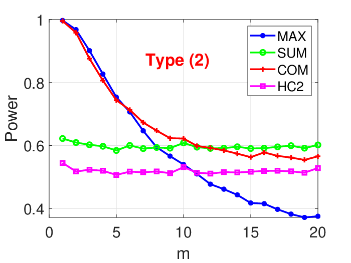

Table S7 reports the empirical sizes of the compared tests. We see that all the tests control the empirical sizes in most cases except that the sizes of HC2 are a little smaller than the nominal level when .
Figure S4 shows the power of each test, where we observe a similar pattern as in Example 1. The power of MAX declines as the number of variables with nonzero means is increasing. The power of SUM and COM are always larger than that of HC2 in all cases. The proposed COM matches the power of MAX when the number of variables with nonzero means is small, and almost has same power as SUM when is large. This justifies the superiority of the proposed combo-type test in the two-sample testing problem, regardless of the sparsity of the data.
S2 Technical Proofs
S2.1 Proof of Theorem 1
Proof of Theorem 1. Let be i.i.d. -distributed random variables. Let be a non-negative definite matrix such that Then and have the same distribution. As a consequence, has the same distribution as that of
| (S.7) |
Let be the eigenvalues of and be a orthogonal matrix such that . In particular, since all of the diagonal entries of are , we have . By the orthogonal invariance of normal distributions, and have the same distribution. By (S.7), is equal to
and hence has the same distribution as that of . It is easy to see and
Easily, for any . Note that is a sum of independent random variables. Then,
which goes to zero by Assumption (1). Therefore, by the Lyapunov central limit theorem, converges weakly to as This implies that converges weakly to as
S2.2 Proof of Theorem 2
For a graph , we say vertices and are neighbors if there is an edge between them. For a set , we write for its cardinality. We first prove some lemmas.
LEMMA S.1
Let be an undirected graph with vertices. Write . Assume each vertex in has at most neighbors. Let be the set of subgraphs of such that each subgraph has vertices and at least one edge. The following are true.
(i) for any .
(ii) Fix integer with . Let such that each member of is a clique, that is, any two vertices are neighbors. Then
The following conclusions are true for integer with .
(iii) For , let be the subset of from satisfying the following: there exists a subgraph of with and without any edge such that any vertex from has at least two neighbors in . Then .
(iv) For , let be the subset of from satisfying the following: for any subgraph of with and without any edge, we know any vertex from has at least one neighbor in . Then
Proof of Lemma S.1. (i). Choose one vertex from and choose one of its neighbors. The total number of ways to do this is . The total number of ways to fill the rest of vertices arbitrarily is no more than . Hence,
(ii). To form a clique from , we first choose a vertex with ways. The next vertex has to be one of its neighbors, the third vertex has to be one of the neighbors of the first two vertices at the same time. Thus the number of choices for the third vertex is no more than . This has to be true for the picks of the remaining vertices to form a clique. So .
(iii). Now we figure out the ways to get . The number of ways to get is at most . Once is chosen, another vertex from its neighbors has to be picked to be an element in . Once is taken, since at leat two members from are neighbors of , a third vertex has to be in . Keep in mind that has to be a neighbor of . Thus, the total number of ways to pick these three vertices is at most The rest of vertices in have at most choices to satisfy the requirement; the rest vertices from have to be the neighbors of the vertices in , which amounts to at most ways to fill the vertices. So
(iv). The choices of with is no more than . Any of the rest vertices from must be the neighbor of a vertex from the chosen vertices. The total number of neighbors is at most . This amounts to no more than ways to achieve this. Hence .
LEMMA S.2
For , let be positive integers with . Let be -distributed random variables with covariance matrix Assume for all and , where are constants satisfying Given , set Then, for any fixed , we have
as uniformly for all
Proof of Lemma S.2. To ease notation, we write “” for “” if there is no danger of confusion. First, is well-defined as is large. Note that , where . Recall the density function of is given by for all . It follows that
| (S.8) |
For two non-negative definite matrices and , we write if is also non-negative definite. We need to understand and on the right hand side of (S2.2). First we claim that
| (S.9) |
and that
| (S.10) |
as is sufficiently large.
In fact, by the Gershgorin disc theorem (see, e.g., Horn and Johnson 2012), all eigenvalues of have to be in the set
By assumption, and for all . Thus, all of the eigenvalues of are between and . The two bounds are positive as is sufficiently large. On the other hand, and as is sufficiently large. The assertion (S.9) is obtained.
Second, is the sum of terms. The term as the product of the diagonal entries of is ; each of the remaining terms is the product of entries from which at least one is an off-diagonal entry. Therefore, This implies . Trivially, as . The statement (S.10) is confirmed.
The claim (S.9) implies that for each The tail bound of Gaussian variable gives as Since for any , for any , there exists such that
| (S.11) |
for all Thus, from (S2.2)-(S.11), we upper bound the probability of interest by
as , where Now
as since , where the last depends on and . Consequently,
where
as is sufficiently large because . In summary, for fixed ,
| (S.12) |
as is sufficiently large. Similarly, from (S2.2)-(S.11), a lower bound can be established as
where By taking care of each term above as in the previous arguments, we can get a reverse inequality of (S.12) with “” replaced by “”. Consequently, we know that
| (S.13) |
as , where is a constant that depends on and only. Now we consider the decomposition
| (S.14) |
where the summation is over all the possible cases with Notice that , and the derivation of (S.13) depends on rather than the exact values of ’s. By (S.14), we have
as . Based on the same reasoning, for any , we have
as uniformly for all Because the probability above does is independent of , by letting and , we have that
as uniformly for all , which completes the proof.
For any symmetric matrix , we use the notation to denote its spectral norm, that is, . Evidently, . Also, if is non-negative definite. Obviously, for any symmetric matrix , if then for any . The same argument applies to . Thus, by symmetry we know that
| (S.15) |
for any The following lemma would be further needed.
LEMMA S.3
Let and be -distributed random variables with positive definite covariance matrix For some , assume , and for all but . Then, if , we have
| (S.16) |
for all , where
Proof of Lemma S.3. Let and
| (S.17) |
Then . We claim that (which will be prove later)
| (S.18) |
for all Assuming this is true, then obviously,
Let . Then . By (S.17), Therefore,
| (S.19) |
for any , where in the last step we use a well-known inequality of the Gaussian tail: for any . Firstly, if , then
It is easy to check that Notice . We have from (S2.2) that
| (S.20) |
So the conclusion holds for . From now on, we assume .
Step 1: the proof of (S.18). Define
where is a matrix whose entries are all equal to zero. Trivially, the eigenvalues of are and , respectively. Basic algebra gives
| (S.21) |
and the eigenvalues of are with folds, and , respectively, which by assumption bounds the spectral norm as Also, since for all but . By the fact that , we obtain
| (S.22) |
In particular, this implies from the triangle inequality that
By assumption , we know . By solving the inequality we obtain . Substituting this to (S.22) we get
| (S.23) |
From (S.17), we know for , where and the only “” appears in the th position. As is positive definite, To show (S.18), it is enough to show for each . Define , which equals the th row sum of . We have
| (S.24) |
induced by (S.23). Therefore, . Now observe from (S.21) that
and for Thus, (S2.2) and condition conclude that for each , which implies (S.18).
Step 2: the proof of (S.16). From (S.15) and (S.23),
As a result, we have
by using the assumption . By assumption , we further obtain
In particular, for Then, we can establish from (S2.2) that
| (S.25) |
under the assumption . In the above derivation, the true values of ’s are not used, instead their bounds and are relevant. Therefore, (S.20) and (S.25) still hold if each “” is replaced by “” with . Trivially, for each . This combining with (S.25) and (S.14) yields (S.16).
To prove Theorem 2, we need a notation. Let and be a non-negative definite matrix. For and a set with , define
| (S.26) |
Specifically, takes possible values , where we regard . If , then for all and
Proof of Theorem 2. For any , write
| (S.27) |
which is well defined as is sufficiently large. We will not mention this matter again since the conclusion is valid as It suffices to show
| (S.28) |
as The proof will be divided into a few steps.
Step 1: reducing “” in (S.28) to a set of friendly indices. First,
| (S.29) |
as , where for two sequences of real numbers and , the notion means that as Immediately, a union bound implies
as , where we recall the definition with . Further denote . By assumption, as . It follows that
Therefore, to prove (S.28), it is enough to show
| (S.30) |
as asymptotically.
Step 2: estimation of via the inclusion-exclusion formula. Set
| (S.31) |
for , where the sum runs over all such that . Then,
| (S.32) |
for any We will prove next that
| (S.33) |
for each Assuming this is true, let in (S.32), we have
for each . By letting and using the Taylor expansion of the function , we obtain (S.30). It remains to verify (S.33). Evidently, by (S2.2) and the assumption , we immediately see (S.33) holds as Now we prove (S.33) for any .
Recalling , we write
where
| (S.34) |
Now, think as graph with vertices, with and by assumption. Any two different vertices from , say, and are connected if In this case we also say there is an edge between them. By the definition , each vertex in the graph has at most neighbors. Replacing “”, “” and “” in Lemma S.1(i) with “”, “” and “”, respectively, we have that for each . Therefore, . Since and as , we know
| (S.35) |
Decomposing (S.31), we see that
From Lemma S.2 and (S.35) we have
as As a consequence, to derive (S.33), we only need to show that
| (S.36) |
as asymptotically for each
Step 3: the proof of (S.36). If , the sum of probabilities in (S.36) is bounded by . By Lemma S.1(i), . Since , by Lemma S.3,
| (S.37) |
uniformly for all as is sufficiently large, where is a constant not depending on We then know (S.36) holds. The remaining job is to prove (S.36) for
Take in (S.26) for the definition of and compare it with from (S.34). To proceed, we further classify into the following subsets
for By the definition of , we know that . Since is fixed, to show (S.36), it suffices to prove
| (S.38) |
for all .
Assume , which implies for all by (S.26). Hence, the subgraph is a clique. Taking , and into Lemma (S.1)(ii), we get . Thus, we obtain
| (S.39) |
Now we assume with . By definition, there exits such that and for each , there exists satisfying . Looking at the last statement we see two possibilities: (i) for each , there exist at leat two indices, say, , with satisfying and ; (ii) there exists for which for an unique . However, for , (i) and (ii) could happen at the same time for different , say, (i) holds for and (ii) holds for simultaneously. Thus, to differentiate the two cases, we consider the following two types of sets. Denote
| (S.40) |
Replacing “”, “” and “” in Lemma S.1(iii) with “”, “” and “”, respectively, we have that for each . Analogously, set
| (S.41) |
From Lemma S.1(iv) we see It is easy to see . Therefore, to show (S.38), we only need to prove both
| (S.42) |
and
| (S.43) |
as for . In fact, let be as in (S.40), then using Lemma S.2, the probability in (S.42) is bounded by uniformly for all as is sufficiently large, where is a constant independent of . This leads to
as is sufficiently large. By the assumption that , we arrive at (S.42).
Finally we validate (S.43). Recall the definition of . For , pick with , and such that for a unique Then each probability in (S.43) is bounded by
for . Taking and applying Lemma S.3, the probability above is dominated by
for some constant . As stated earlier, by union bound, since , we see the sum from (S.43) is of order . Hence, (S.43) holds. We have proved (S.38) for any , which concludes the proof.
S2.3 Proof of Theorem 3
The proof of Theorem 3 is involved. A preparation with a few of lemmas is given below.
LEMMA S.4
Let and be nonnegative definite matrices. Then
Proof of Lemma S.4. Assume and are matrices. There is an orthogonal matrix such that , where and Observe , and . Thus, without loss of generality, we assume . Write . Then, for each and
The proof is completed. .
The following is a well-known formula for the conditional distributions of multivariate normal distributions; see, for example, p. 12 from Muirhead 1982.
LEMMA S.5
Let with being invertible. Partition and as
| (S.44) |
where . Set . Then and is independent of .
LEMMA S.6
Let . Under the notion of Lemma S.5, for , write and . Define and . Assume with for each , where is a constant depending on only. Then there exists a constant free of , and , such that the following holds:
(i) for all where
(ii) for all .
(iii) for .
Proof of Lemma S.6. Set , so is , is and is . Let and , where the random variables ’s and ’s are i.i.d. -distributed. According to Lemma S.5,
| (S.45) |
and they are independent. From (S.45) we see that , where
By the singular value decomposition theorem, we write where are the singular values of , and and are orthogonal matrices. Review the well-known facts that
| (S.46) |
for any matrices and and any non-negative definite matrices and (the second fact from (S.46) can also be thought as a consequence of Lemma S.4). Note that
| (S.47) |
and all three matrices are non-negative definite. This together with the Weyl interlacing inequality implies . Consequently, we have from Lemma S.4 that
Furthermore, by Lemma S.4 again,
| (S.48) |
In fact in the above we use the assertion by the Weyl interlacing inequality and the fact that
by assumption. Combing the above, we arrive at
| (S.49) |
Another fact we will use later on is that
| (S.50) |
In fact, recall that denotes the spectral norm of a matrix. By definition,
| (S.51) |
From (S.47) we know that both norms in (S2.3) are bounded by So (S.50) is obtained. With these preparation, we are ready to prove (i), (ii) and (iii).
(i) Since and , by the orthogonal invariant property of , we have that
| (S.52) |
Review the moment generating functions of Gaussian variables,
| (S.53) |
We can write
for all with , that is, . Notice as , Thus, there exists such that for all . Then
| (S.54) |
for all with by (S.49), with The inequality (S.54) is particularly true if by (S.50).
(ii) Let be the eigenvalues of From (S.47) we have
| (S.55) |
By (S.45) and the orthogonal invariant property of normal distributions similar to (S.52),
| (S.56) |
As shown in (S2.3),
| (S.57) |
for all . Recalling defined earlier, we conclude
for all . By (S.55), the above is particularly true provided , which proves the claim.
(iii) By the Hölder inequality and the fact that for each ,
for all For defined earlier, we obtain
for as desired.
LEMMA S.7
Proof of Lemma S.7. First we give an estimate for Set , where is the constant as given in Assumption (2). Evidently, . Also and for each by Assumption (2). It follows that
| (S.59) |
for . Now, for any , union bound gives
| (S.60) |
Let us bound them one by one. First, by the Markov inequality and Lemma S.6(ii),
| (S.61) |
for any where is a constant free of . By assumption, and . Then,
| (S.62) |
due to (S.59). Thus, (S.58) holds. Choosing , we see from (S2.3) that
| (S.63) |
for all satisfying , which is particularly true if
| (S.64) |
Second,
By Lemma S.6(i) and a similar argument as (S2.3), we have
for all , where It is trivial to see from the notation that . Take to obtain
| (S.65) |
for all satisfying (S.64). Finally, by the Markov inequality and by taking from Lemma S.6(iii) we obtain
for every satisfying , or equivalently, . In the last step above we use the inequality from (S.59). Combining this with (S2.3), (S.63) and (S2.3), we conclude that
for every satisfying from (S.64) and .
We now introduce more general indexing. Let . Assume is an integer with . For any set with , write . Let be the vector obtained with deleting from , that is, where and Let be the covariance matrix of
Partition similar to (S.44) such that
In particular, and . We have the following result.
LEMMA S.8
Let . Assume is an integer with . For any set with , we define and . Set and . Then, under Assumption (2), for any there exists such that
as is sufficiently large, where the maximum runs over all possible indices with .
Proof of Lemma S.8. View as the vector after exchanging some rows of . Then there is a permutation matrix such that . Therefore the covariance matrix of is Set . Then
| (S.66) |
Second, is the matrix by exchanging some rows and then exchanging the corresponding columns. So the entries of are the same as those of ; the sum of squares of the entries of a row from is the same as that of a row from , and vice versa. Write . As a consequence,
| (S.67) |
Notice that in Assumption (2), all conditions are imposed on the four quantities: , , and . As a result, by (S.66) and (S.67), we see that (2) still holds if “” is replaced with “”. Review Lemma S.7. Let be as in (2). Let be as in (S.58). By this display,
as . Evidently, and . Thus
if . Taking such that , and for all and applying Lemma S.7, we know that
| (S.68) |
as . Note that in the proof of (S.68), although the conclusion is on , only five quantities of in (S.66) and (S.67) are required, and they are the same if “” is replaced by “” for different Consequently, we induce from (S.68) that
for any and any with . The desired conclusion then follows by writing back to .
LEMMA S.9
Proof of Lemma S.9. We prove the lemma in two steps.
Step 1: appealing independence from normal distributions. Note that . Take and . Recall the notation in Lemma S.5, which allows us to write
where and . Lemma S.5 says that
| (S.69) |
Further denote
We will show the last three terms on the right hand side are negligible. Recall
as defined in Lemma S.7. By Lemma S.8 with , for any and , there exists with and integer , such that
| (S.70) |
as . Now for clarity we re-write the definition of as
for . Since , we see that
by the independence stated in (S.69). Regarding the first probability, we have
Combine the two inequalities to get
| (S.71) |
Similarly,
By the independence from (S.69),
Furthermore,
where the fact is used again. Combining the above two inequalities we get
This together with (S.71) implies that
| (S.72) |
as , where
since is increasing in An important observation is that the derivation of (S2.3) is based on three key facts: inequality (S.70), the identity and the fact and are independent from (S.69).
Recall the notations in Lemma S.8. For any , denote . Then, . By Lemma S.5, and are independent. In addition,
Hence, we can write . Based on Lemma S.8,
when . Consequently, the three key facts aforementioned also hold for the corresponding quantities related to . Thus, similar to the derivation of (S2.3), we have
as . Taking the summation we get
| (S.73) |
where we denote
In the following we will show and for each . Assuming these are true, by using and (S2.3), for fixed , by sending first and then sending , we obtain for each . The proof is then completed.
Step 2: the proofs of “ ” and “ for each ”. First, as discussed below (2), Assumption (2) implies Assumption (1). Thus, Theorem 1 holds and we have as ,
| (S.74) |
and hence
| (S.75) |
as , where . This implies that .
Second, take Recall for defined in Theorem 2. By Assumption (2), we know for all . Then
for each . This implies that . Take for . Then, and , which gives
| (S.76) |
Hence, Recall (S.27), (S.31) and (S.33). By noting that “” here is exactly “” there for each , we know
| (S.77) |
for each The proof is finished.
We are now in the position to prove Theorem 3.
Proof of Theorem 3. Again, since Assumption (2) implies Assumption (1) and Assumption (2), we know that Theorem 1 and Theorem 2 hold. Set . By Theorem 1,
| (S.78) |
as for any , where . From Theorem 2, we have
| (S.79) |
as for any To show asymptotic independence, it is enough to prove
for any and . Define
| (S.80) |
where the latter one makes sense for sufficiently large . Due to (S.78), the above condition we want to prove is equivalent to
| (S.81) |
for any and . Recalling the notation in Lemma S.9, we have
| (S.82) |
for . We can then write
| (S.83) |
Here the notation stands for . From the inclusion-exclusion principle,
| (S.84) |
and
| (S.85) |
for any integer . As in the proof of Lemma S.9, define
for . From (S.77) we know
| (S.86) |
Denote
By Lemma S.9, we have
| (S.87) |
for each . The assertion (S.84) implies that
| (S.88) |
where the inclusion-exclusion formula is used again in the last inequality, that is,
for all . By the definition of and (S.79),
as . By (S.78), as From (S.83), (S.87) and (S2.3), by fixing first and sending we obtain that
Now, by letting and using (S.86), we have
| (S.89) |
We next prove the lower bound in a similar way. By applying the same argument to (S.85), we see that the counterpart of (S2.3) becomes
where in the last step we use the inclusion-exclusion principle such that
for all . Review (S.83) and repeat the earlier procedure to see
with and , which, together with (S.89), yields (S.81). The proof is now complete.
S2.4 Proof of Theorem 4 and Theorem S6
LEMMA S.10
Let and be two sequences of random variables with and in distribution as Assume and are continuous random variables and
| (S.90) |
If and are asymptotically independent, then and are also asymptotically independent.
Proof of Lemma S.10. Define
for any and . By (S.90),
| (S.91) |
for any . Fix and . We note that
| (S.92) |
By the assumption on the asymptotic independence,
| (S.93) |
for any and . By letting and then in (S2.4), since and are continuous, we deduce from (S.91) and (S.93) that
| (S.94) |
By switching the roles of “ and ” and “ and ”in (S2.4), we have
for any , and . Or, equivalently,
Similar to the derivation of (S.94), we get
This and (S.94) lead to
which shows the asymptotic independence between and as claimed.
Proof of Theorem 4. By Theorem 3.1 in Srivastava 2009, we get claim (i). We next prove claim (ii).
Recall are i.i.d. -distributed random vectors and . Note that under the null hypothesis in (4). Write , and let denote the population correlation matrix, where is the diagonal matrix of . Then for each and for In other words, . By assumption, (2) holds with “” replaced by “”. Set . Since Assumption (2) is stronger than Assumption (2), by Theorem 2 and Assumption (2), it holds that
| (S.95) |
Observe that the distribution of is free of , hence the above limit holds for any . Now, to prove (ii), we only need to show that . Indeed, we have
| (S.96) |
First, use the inequality for to see
Thus,
| (S.97) |
Based on the explanation below (8), we have
| (S.98) |
for each . Set with the constant to be determined. Then
by considering or not. Recall the Chernoff bound and the moderate deviation for sum of i.i.d. random variables (see, for example, p.31 and p.109 from Dembo and Zeitouni 1998). There exists a constant such that for all and
| (S.99) |
as is sufficiently large, where and the fact is used in the last step. Choose to bound the above probability by . It follows that
as . This says
| (S.100) |
This together with (S2.4) and (S.97) implies as long as . This confirms , and the proof of part (ii) is completed by using (S2.4).
Finally we prove part (iii). According to the proof of Theorem 3.1 in Srivastava 2009 or the proof of Theorem 1 in Jiang and Li 2021, we have
| (S.101) |
Also, using an conclusion from the proof of (ii) above,
| (S.102) |
Since , then by using the notation Recall an earlier notation for each . Obviously, . We are able to rewrite (S.101) and (S.102) in terms of ’s as
As aforementioned, Assumption (2) is stronger than Assumption (2). We then conclude (iii) by Theorem 3, Lemma S.10 and the fact .
Verification of . Recall the simplified assumption that , and . In this case, . We also assume that . Because of the condition , we know . As a consequence, the requirement on vs imposed in Theorem 4(ii) is satisfied. Notice is equal to
Since by assumption, we have from (S.100) that . In particular, we have from the triangle inequality that
| (S.103) |
From the fact , we see
According to Theorem 4(ii), we have . This and (S.103) conclude that
Thus,
which goes to The verification is completed.
Proof of Theorem 6. The proof shares same spirit as Theorem 4. Denote . According to Section 5 in Srivastava and Du 2008 or Theorem 2 in Jiang and Li 2021, (i) holds. We prove (ii) next.
Under the normality assumption and the null hypothesis in (S.1), we have . Let be the diagonal matrix of . Recall Then
| (S.104) |
According to Section 5 and the proof of Theorem 2.1 in Srivastava and Du 2008 or the proof of Theorem 2 in Jiang and Li 2021, we have
| (S.105) |
Let be the th coordinate of for and . Then
Recall
where is the th diagonal element of in (S.3). Set
Then Recalling the discussion below (2), Assumption (2) is stronger than Assumption (2). By Theorem 2 and Assumption (2), we obtain
| (S.106) |
Thus, to prove (ii), it suffices to show that . By (S.3), follows a Wishart distribution with parameter and covariance matrix . Since is the th diagonal element of , we know , or equivalently,
for each By the same argument as between (S.98) and (S.100), we have from the above assertion that . Notice (S2.4) implies . By the triangle inequality of the maximum and the trivial inequality for any and , we get
| (S.107) |
Consequently, (ii) follows from (S2.4) under the assumption .
S2.5 Proof of Theorem 5
To prove Theorem 5, we need a preparation. In fact, an asymptotic ratio-consistent estimator of will be derived (the notation of “” is given in (S.109)). It is stated in Proposition S1. We will develop a series of auxiliary results for this purpose.
Review the setting in Section 3.2. In what follows, we assume the integers , and satisfy and .
LEMMA S.11
Let be i.i.d. from the -dimensional distribution Write
for each , where is a -dimensional vector with distribution . Then is a matrix. Recall in (16). We then have
where is a matrix and the entries are i.i.d.
Proof of Lemma S.11. Recall the notation between (15) and (16),
where is , is , both and are and is . is defined as
| (S.108) |
Then, by Lemma S.5, the -dimensional random vector and is independent of . It follows that the conditional distribution of given is characterized by
Therefore, we have from the definition that
| (S.109) |
Write
Notice the last two vectors are both normal and they are independent since that are i.i.d. from the -dimensional population . Moreover, we can also write
| (S.110) |
where are i.i.d. -dimensional random vectors with distribution also independent of . By definition (S.108),
| (S.111) |
since . Let be i.i.d. -distributed random variables independent of . Without loss of generality, assume for each . Therefore,
| (S.112) |
Since the idempotent matrix has rank , we know has rank . As a function of , is independent of . As a result, there exists an random orthogonal matrix independent of such that
where the three above are matrices of entries with proper size. By the orthogonal invariance of i.i.d. standard normals, has the same distribution as that of . From (S2.5) and (S.112), we have
where .
LEMMA S.12
Proof of Lemma S.12. Let be a matrix whose entries are i.i.d. Immediately, . Using the identity for any matrices and , we know that
| (S.114) |
and
| (S.115) |
Since are the eigenvalues of , we are able to decompose , where is an orthogonal matrix and . By the orthogonal invariance of i.i.d. -entries, we get
Furthermore write . Then are i.i.d. -dimensional vectors of distribution . Hence,
which gives
| (S.116) |
Additionally, we have
Observe
Similarly, . Then we end up with
It follows from (S2.5) that
| (S.117) |
Since are i.i.d. , we know and , where and is independent of . Recall and for any integer . Thus, by independence we have From (S.117), we obtain
Using the identity
we arrive at
by using (S.109). This completes the proof of the lemma.
LEMMA S.13
Let and and be i.i.d. -dimensional random vectors with distribution . Then the following are true.
(i)
(ii)
(iii) .
(iv)
Proof of Lemma S.13. It is well-known that
| (S.118) |
for all integers . We will use this formula to prove the results.
(i) Since , we have
| (S.119) |
and . This leads to
(ii) By Proposition 7.3 from Eaton 1983 or Theorem 1.5.6 from Muirhead 1982, it holds that
| (S.120) |
for . Therefore, , where and is independent of . Consequently, by (S.119),
(iii) By (S.120), we have
Easily, be checking their covariance, we know and are i.i.d. . This implies that , and are independent. Thus, from (S.119) we obtain
(iv) Write . From the independence between and , we conclude that
Thus, the verification is completed.
Proof of Lemma S.14. Set and . Let be the eigenvalues of . Standard computation gives
| (S.121) |
for any random variables . Then, from Lemma S.12 we see
| (S.122) |
where . By Lemma S.13(i),
| (S.123) |
By Lemma S.13(ii),
| (S.124) |
By Lemma S.13(iii),
| (S.125) |
By Lemma S.13(iv),
| (S.126) |
Let be uniformly distributed over By Hölder’s inequality, for any . This says that
By taking , respectively, and , we have
| (S.127) |
for Consequently,
Combing the above with (S2.5), we get
Using the fact to see and plugging in and , we obtain
which concludes the proof.
LEMMA S.15
Proof of Lemma S.15. Set and . Let be the eigenvalues of the matrix . Let be i.i.d. random variables with distribution , with and . From (S.116),
| (S.128) |
Let be a random variable with mean . Write . Trivially, for any random variables and . Then
Now consider to be , with . Use (S.127) to see
| (S.129) |
By the Marcinkiewtz-Zygmund inequality [see, e.g., Theorem 2 on p. 386 from Chow and Teicher 1997] and the Cauchy-Schwartz inequality, we obtain
where is a numerical constant. Write , where are i.i.d. -distributed random variables. By Corollary 2 on p. 387 from Chow and Teicher 1997, , where is also a numerical constant. That is, . In summary, we get and hence
from (S.128) and (S.129). The conclusion then follows by using the fact .
PROPOSITION 1
Proof of Proposition 1. Since for any random variables and , by Lemma S.14 and Lemma S.15, there exists a constant independent of or such that
| (S.130) |
On the other hand, by (S.113),
| (S.131) |
Define . Let be the eigenvalues of the matrix . By (S.116),
where are i.i.d. -distributed random variables. From (S.119), . Thus, we have from independence that
or equivalently,
Combine this with (S2.5) to get
| (S.132) |
where . Under Assumption (20), for some constant . This then implies
We deduce from (S2.5) and (S.132) that
where the fact is used in the second inequality. Under the conditions , and , we know and , hence the last term is of order . This leads to in probability and we conclude from (S.132) that
in probability. The proof is complete.
LEMMA S.16
Let be i.i.d. -dimensional random vectors with distribution , where is a non-negative definite matrix. Let be a non-zero random vector independent of . Write and the matrix . Then and is independent of .
Proof of Lemma S.16. Write and . Use the fact that the rows of the matrix are i.i.d. to see if and if . Thus,
| (S.133) |
Obviously, for each . Since is a unit random vector, then conditional on , we know are jointly Gaussian random variables with for each . Let us check their covariance matrix. In fact, conditional on ,
by (S.133) and the fact . In summary, conditional on , the random vector . Since is free of , this implies, unconditionally, it is also true that . Finally, for any set and ,
This shows that and are independent.
LEMMA S.17 (Bai and Silverstein 2010)
Let be an non-random matrix and be a random vector of independent entries. Assume that , and . Then, for any ,
where is a constant depending on only.
LEMMA S.18
Assume satisfies that are i.i.d. with , and for an integer . Let be an symmetric, random matrix satisfying and . Assume and that and are independent. Then
(i) ;
(ii) , where is a constant depending on only.
Proof of Lemma S.18. It is easy to see for any matrix .
(i) Obviously, the conditional mean Take another expectation to see By Lemma S.17,
where is a constant free of . By taking another expectation, we get . Thus, by the Chebyshev inequality,
This implies .
(ii) First, . Trivially,
From Lemma S.17 and the fact for any , we see
where is a constant depending on only. Therefore,
| (S.134) |
where is a constant depending on only. On the other hand, noting that the entries of are i.i.d. , by conditioning on and , the random variable has the distribution of , where . Or, equivalently,
In particular, this implies that
By combining this, (S.134) and the fact , we obtain
The proof is completed.
Recall random error vector in the linear regression model from Section 3.2. The components are assumed to be i.i.d. random variables.
PROPOSITION 2
Proof of Proposition 2. Recall the notation between (15) and (16). In particular, . Under the null hypothesis in (14), , where and the random errors are i.i.d. with and for each . Also, is assumed to be independent of . Use and to see
| (S.135) |
Recalling (16), we denote
| (S.136) |
where and are matrices. Write . Then the last assertion from (S.136) says that for each . This leads to
via the facts and again. Note that is a scalar. By the definition of in (18), we derive
Set
By the triangle inequality,
| (S.137) |
Define
By Lemma S.18(i), we know , which implies
| (S.138) |
We will show that, as ,
| (S.139) | ||||
| (S.140) |
Assuming they are true, using assumption and (S2.5) we have
| (S.141) |
This and (S.139) show that converges weakly to a distribution with cdf , . It remains to prove (S.139) and (S.140), which will be done in two steps as follows.
Step 1: the proof of (S.139). By (S.110) and (S.136), , where are i.i.d. -dimensional random vectors with distribution and they are also independent of . In particular, are independent of , a function of . As , we see that
Write . In other words, each is a column of . Immediately we have
| (S.142) |
for each This means , which then leads to
| (S.143) |
by using the fact Obviously, it holds that
| (S.144) |
A key observation is that the three random quantities , and are independent. By the last assertion from (S.142) and Lemma S.18(ii), we have
| (S.145) |
for any , where and is a constant depending on only. We next show
| (S.146) |
in probability as . In fact, for any ,
Therefore, from assumption for some , we have
where is a constant depending on and . Since , we get the first limit of (S.146) by using the assumption . For the second limit, by setting we have
By the law of large numbers, in probability. Thus, to get the second limit of (S.146), it suffices to prove
| (S.147) |
in probability. Similar to an earlier argument, we have from the fact that
by the Cauchy-Schwartz inequality and , where is a constant depending on and only. Use (S.145) to see
by the assumption again. Since and , we get (S.147) and then the second limit of (S.146).
Now we study in (S2.5). Since are i.i.d. with mean zero and variance . By assumption, with . This concludes . Write . By the central limit theorem, . Use to see
| (S.148) |
Review are i.i.d. -dimensional random vectors with distribution and . By Lemma S.16,
| (S.149) |
Based on assumption, (2) holds with “” replaced by “”, we know Assumption (2) also holds by the discussion below (2). We then have from Theorem 2 that
as . Denote . Then the above says converges weakly to the Gumbel distribution with cdf . It then follows from (S2.5) that
Obviously, the last term goes to zero since by assumption. Use the Slutsky lemma to see that
converges weakly to the Gumbel distribution with cdf . We then obtain (S.139) by (S2.5) and (S.146).
Step 2: the proof of (S.140). Easily, by definition,
By (S.139), . Thus, to prove (S.140), it suffices to show
| (S.150) |
Now we prove this assertion. From assumption for some , we choose This indicates that
| (S.151) |
Note that, for and satisfying , one of the two inequalities and must hold. Equivalently, or . Both of them imply that . Consequently,
Recalling (S.142) and that the matrix has rank , we know Denote . Observe that implies , which implies . Use (S.151) and the assumption to see By definition, . Similar to (S.99), we have
which is equal to by assumption . This says , which implies (S.150), and hence (S.140) holds as aforementioned.
Recall the error vector in the linear regression from Section 3.2. We assume are i.i.d. random variables.
PROPOSITION 3
Proof of Proposition 3. Recall the notation from Section 3.2. In particular,
and
| (S.152) |
Next we will first derive a workable form for the main ingredient above.
Recall . Under the null hypothesis in (14), , where , and are i.i.d. random variables with and . By assumption, are also independent of . Recalling (S.136), we denote
Since , both and . Thus, . By definition,
| (S.153) |
and
It is easy to verify that . Consequently,
| (S.154) |
According to (S.142), and . Hence,
| (S.155) |
where . Eventually, we arrive at an ideal form to work with, that is,
| (S.156) |
Now we start to prove the central limit theorem. The assumption with implies that with . It follows from Lemma S.18(i) that
| (S.157) |
This and (S.153) imply that
| (S.158) |
By assumption for some , we see
| (S.159) |
with .
In lieu of the explanation before (S.142), are independent of and , and hence are independent of the unit random vector . We then have from Lemma S.16 that has distribution and is also independent of . By assumption, (2) holds with “” replaced by “”. From Theorem 1 and (S.109) we have
| (S.160) |
in distribution as From (S.153), we know . By (S.156) and (S.160) we have
Use the fact to see
| (S.161) |
By Proposition 1, in probability. We then arrive at
through an application of the Slutsky lemma. The proof is completed.
Proof of Theorem 5. Parts (i) and (ii) follow from Propositions S3 and S2, respectively. The setting here is the same as those in the two propositions, so we will continue to use the same notation in the two propositions to prove (iii) for the asymptotic independence. Recall the definition
By (S.153) and (S.156), we have
Thus,
where
By Proposition 1, in probability. Hence in probability. Also, by (S.160). This together with the assumption for some implies that
| (S.162) |
On the other hand, based on (S.139) and (S2.5),
| (S.163) |
by(S.155). Remember that is independent of because are independent. It follows that
| (S.164) |
According to (S.159), we know that
with . As a consequence,
| (S.165) |
From the discussion between (S.159) and (S.160), it holds that
| (S.166) |
By assumption, (2) holds with “” replaced by “”, we know Assumption (2) also holds by the discussion below (2). Due to Theorem 2, we get
for any as . By assumption, , the above particularly implies . This together with (S2.5) and (S.165) concludes that
According to (S2.5), we have
Joining this with (S.162) and (S.166), by Theorem 3 and Lemma S.10, we obtain and are asymptotically independent.