A Flexible Approach for Predictive Biomarker Discovery
Abstract
An endeavor central to precision medicine is predictive biomarker discovery; they define patient sub-populations which stand to benefit most, or least, from a given treatment. The identification of these biomarkers is often the byproduct of the related but fundamentally different task of treatment rule estimation. Using treatment rule estimation methods to identify predictive biomarkers in clinical trials where the number of covariates exceeds the number of participants often results in high false discovery rates. The higher than expected number of false positives translates to wasted resources when conducting follow-up experiments for drug target identification and diagnostic assay development. Patient outcomes are in turn negatively affected. We propose a variable importance parameter for directly assessing the importance of potentially predictive biomarkers, and develop a flexible nonparametric inference procedure for this estimand. We prove that our estimator is double-robust and asymptotically linear under loose conditions on the data-generating process, permitting valid inference about the importance metric. The statistical guarantees of the method are verified in a thorough simulation study representative of randomized control trials with moderate and high-dimensional covariate vectors. Our procedure is then used to discover predictive biomarkers from among the tumor gene expression data of metastatic renal cell carcinoma patients enrolled in recently completed clinical trials. We find that our approach more readily discerns predictive from non-predictive biomarkers than procedures whose primary purpose is treatment rule estimation. An open-source software implementation of the methodology, the uniCATE R package, is briefly introduced.
Keywords Heterogeneous treatment effects High-dimensional data Nonparametric statistics Precision medicine Predictive biomarkers Variable importance parameter
1 Introduction
Precision medicine is now a chief focus of the biomedical establishment. Its promise of tailored interventions and therapies is impossible to overlook, potentially spelling major improvements in patient outcomes (Kraus 2018; Ginsburg and Phillips 2018). Much effort has therefore been invested in the development of quantitative methods capable of uncovering patient sub-populations which benefit more, or less, from novel therapies than the standard of care.
These groups of patients are distinguished from one another based upon diverse biometric measurements referred to as predictive biomarkers (Royston and Sauerbrei 2008; Kraus 2018). Examples include age, sex at birth, ethnicity, and gene expression data taken from various tissue samples. Once identified, these biomarkers may provide clinicians and biologists with mechanistic insight about the disease or therapy, and spur the development of diagnostic tools for targeted treatment regimes.
The statistical discovery of predictive biomarkers has, to date, largely been a byproduct of conditional average treatment effect (CATE) estimation. This typically unknown parameter contrasts the expected outcomes of patients under different treatments as a function of their characteristics, thereby defining the optimal treatment rule. Employing an estimate of the CATE, clinicians can identify a subgroup of patients that draws most benefit from a therapy. When estimated using sparse modelling or otherwise interpretable methods, interpretable machine learning algorithms can be used to find potentially predictive biomarkers (Robins et al. 2008; Tian et al. 2014; Luedtke and van der Laan 2016; Chen et al. 2017; Zhao et al. 2018; Wager and Athey 2018; Fan et al. 2020; Bahamyirou et al. 2022; Hines et al. 2022a).
While CATE estimation procedures are demonstrably successful at predictive biomarker discovery in settings where the number of features is small relative to the sample size, it is not so in modern clinical trial in which the number of features frequently exceeds the number of enrolled patients. The high-dimensional nature of trial data make the CATE estimation problem particularly difficult. Methods proposed for this setting must rely on convenient — and sometimes unverifiable — assumptions about the underlying data-generating process. Examples are sparsity, linear associations, and negligible dependence structures (Tian et al. 2014; Chen et al. 2017; Zhao et al. 2018; Fan et al. 2020; Bahamyirou et al. 2022). When these assumptions are violated, as is the case when, for example, the set of biomarkers is comprised of gene expression data, the CATE estimate will be biased but may be viable. The biomarkers designated as predictive, however, will likely be false positives (as demonstrated in Section 4).
Hines et al. 2022a recently proposed a collection of variable importance parameters that assess the impact of variables, either individually or in predefined sets, on the variance of the CATE. These parameters are based on popular variable-dropout procedures and on previous work about the variance of the conditional treatment effect (Levy et al. 2021). While the proposed estimators of these parameters are consistent and asymptotically linear under non-restrictive assumptions about the data-generating process, Hines et al. 2022a note that quantifying treatment effect modification in this way is misleading when variables are highly correlated. Dropout-based importance metrics may also be deceiving when there are many variables; other features may act as surrogates for the omitted covariate(s) (Hastie et al. 2009, Chap. 15). This framework is therefore inappropriate for the discovery of predictive biomarkers in high dimensions.
Still other procedures not relying on CATE estimation have recently been proposed. Sechidis et al. 2018 developed an information-theoretic approach for identifying these treatment effect modifiers, though the statistical properties of the procedure are not established and the simulations do not consider high-dimensional data. Zhu et al. 2022 recently developed a penalized linear modelling method for the identification of predictive biomarkers in high dimensions that accounts for the biomarker correlation structure. Like the previous method, however, no formal statistical guarantees are provided.
Myriad methods attempting to identify high-dimensional interactions more generally might also be considered for our task (Hao and Zhang 2014; Jiang and Liu 2014; Tang et al. 2020, for example,). They too generally rely on untenable simplifying assumptions about the data-generating process. These include, but are not limited to, assumptions of normality, sparsity of the main effects, sparsity of interaction effects, and bounds on the condition number of the biomarker covariance matrix. Large sets of biomarkers are again unlikely to satisfy such conditions, barring these methods’ use for predictive biomarker discovery in high-dimensions.
A simpler alternative is to fit individual (generalized) linear models of the outcome for each biomarker. Each model is comprised of the biomarker’s main effect and a treatment-biomarker interaction term. The effect size estimate of the latter serves as a measure importance; larger magnitudes equate to increased treatment effect modification. Hypothesis testing about these treatment-biomarker interaction effects is also possible. As with CATE estimation methods, however, this simple approach imposes stringent parametric conditions on the data-generating process. When the outcome is continuous, for example, inference is only possible when all marginal biomarker-outcome relationships are truly linear. In small samples, an additional assumption of Gaussian error terms is needed for valid hypothesis testing. Violation of these unrealistic conditions again produces unreliable predictive biomarker identification.
A lack of Type-I error control has marked repercussions in many biomedical applications. In drug target discovery, limited resources are wasted by performing biological follow-up experiments on false positives. In diagnostic development, the inclusion of non-predictive biomarkers may dilute the signal from truly informative ones. In a sequencing-based diagnostic, invalid biomarkers will compete with others for sequencing reads, reducing the sequencing depth and, thereby, the quantification accuracy of predictive biomarkers. These failings have direct, detrimental effects on patient health outcomes.
Motivated by these drawbacks, we present in this work a flexible approach for directly assessing the predictive potential of individual biomarkers. That is, we estimate (a transformation of) each biomarker’s univariate CATE, a novel variable importance parameter for treatment effect modification. What is more, our procedure permits the formal statistical testing of these biomarkers’ predictive effects under non-restrictive assumptions about the underlying data-generating process, and we find that it controls the false discovery rate (FDR) at the nominal level for realistic sample sizes. We also demonstrate on real-world data that our method provides reasonable sub-population identification results when combined with standard clustering approaches.
We emphasize that our framework is not a competitor of treatment rule estimation procedures, it is complementary. The estimation of the CATE and the identification of predictive biomarkers are related but distinct pursuits. To highlight this, we might consider a two-step procedure wherein the full set of biomarkers is filtered using our method, and then the CATE is estimated using the remaining features. The benefits of such a strategy are numerous. The results of the initial stage can help assess whether the assumption of sparsity used by existing methods is tenable, and therefore whether estimating the CATE is feasible. If not, then the ranking of biomarkers might still provide biological or clinical insight, or motivate further study. If so, the CATE may be estimated more accurately, thanks to the reduced number of features considered, using flexible methods like those of Tian et al. 2014, Luedtke and van der Laan 2016, or Wager and Athey 2018. Further, the rankings generated in the initial stage can impart intuition about the otherwise uninterpretable treatment rule produced by “black-box” methods.
The remainder of the manuscript is organized as follows: In Section 2, the estimation setting and problem are detailed in statistical terms. Section 3 then describes the proposed inferential procedures. The asymptotic behavior of our method is then verified empirically through a comprehensive simulation study in Section 4. Application of the proposed approach to clinical trial data then follows in Section 5. We end with a brief discussion of the method in Section 6. Throughout, we emphasize inference about the univariate CATEs in a randomized control trial setting, though some remarks on its application to observational data are also provided.
2 Variable Importance Parameters
Consider identically and independently distributed (i.i.d.) random vectors , , corresponding to complete but unobserved data generated by participants in an idealized randomized control trial or observational study. We drop the indices for notational convenience where possible throughout the remainder of the article. Here, is a -length random vector of pre-treatment covariates, , like location and income, and pre-treatment biomarkers, , such as gene expression data, is a binary random variable representing a treatment assignment, and and are random variables corresponding to the potential outcomes of clinical interest under both treatment and control conditions, respectively (Rubin 1974). The number of biomarkers is assumed to be approximately equal to or larger than . Generally, only one potential outcome is observed per unit. We ignore this point for now, and return to it in the next section.
Clinically relevant predictive biomarkers are often those that have a strong influence on the outcome of interest on the absolute scale. As such, an ideal target of inference when these outcomes are continuous and the number of covariates small is the CATE conditioning on the set of biomarkers:
For reasons previously discussed, however, accurate and interpretable estimation of this parameter is generally challenging when is large, preventing the accurate recovery of predictive biomarkers.
Indexing the biomarkers of by , such that , centering them such that , and assuming that , we instead target the full-data variable importance parameter where
| (1) |
Under the assumption that the mean difference in potential outcomes admits a linear form when conditioning on any given , is the vector of expected simple linear regression coefficients produced by regressing the difference in potential outcomes against each biomarker. While the true relationship between the difference of potential outcomes and a predictive biomarker is almost surely nonlinear, is a generally informative target of inference. Biomarkers with the largest absolute values in generally modify the effect of treatment the most.
Analogous simplifications of the high-dimensional regression problem are applicable to other types of outcome variables. For binary outcomes, we might similarly wish to quantify the importance of biomarkers on the absolute risk scale using a slightly modified univariate CATE parameter, , where:
| (2) |
for centered biomarkers . This is, in fact, the same parameter as but presented in a more intuitive form for the binary outcome context: assuming a linear relationship between the difference of the potential outcomes’ probability of success and the covariates, this variable importance parameter consists of the simple linear regression coefficients of the difference in the conditional potential outcome success probabilities regressed on each biomarker. Again, the true relationship between the difference of potential outcome probabilities and covariates is unlikely to be linear. Nevertheless, this parameter is telling of biomarkers’ predictive capacities.
We stress that the parameters in Equations (1) and (2) are reasonable approximations of all but pathological treatment effect modification relationships; they summarize the true, marginal functional parameters using interpretable linear models. A case in which will fail to capture treatment effect modification due to biomarker is when the is parabolic: the orthogonal projection of onto produces a variable importance parameter value of zero. If such relationships are suspected, however, it suffices to target the corresponding variable importance parameters of the squared biomarkers. Analogous parameters based on transformations of the biomarkers should be considered when the data-generating process is assumed to possess other similarly troublesome nonlinearities.
3 Inference
As previously mentioned, only one of the potential outcomes, or , is observed per unit. Instead of , we have access to i.i.d. random observations , where and and are defined as before, and is a continuous or binary random outcome variable. is the unknown data-generating distribution of the observed data that is fully determined by and the (conditional) treatment assignment distribution . That is, is an element of the nonparametric statistical model . In a perfect RCT, . The challenge therefore lies in estimating the full-data, causal parameter of Equations (1) and (2) with the observed data; it is generally impossible without making additional assumptions about . We begin by providing such identification conditions.
Throughout the remainder of the text, we represent the empirical distribution of by , the conditional outcome regression function by , and the treatment assignment mechanism by . Where possible, we simplify notation further by writing and as and , respectively. All proofs are provided in Section S1 of the Appendix.
(A1)
No unmeasured confounding: for .
(A2)
Positivity: There exists some constant such that .
A1 assures that there are no unmeasured confounders of treatment and outcome, allowing for treatment allocation to be viewed as the product of a randomized experiment. A2 is an overlapping support condition stating that all observations may be assigned to either treatment condition regardless of covariates. These conditions, regularly cited in the causal inference literature, are generally satisfied in randomized control trials. Altogether, they lead to the following result:
Theorem 1.
Having established the conditions under which can be estimated from the observed data, we now focus on inference about . The EIF of Equation (5) informs the construction of nonparametric efficient estimators of under non-restrictive assumptions about the data-generating process (Bickel et al. 1993; Hines et al. 2022b). Many approaches exist for deriving these efficient estimators, such as one-step estimation (Pfanzagl and Wefelmeyer 1985; Bickel et al. 1993), estimating equations (van der Laan and Robins 2003; Chernozhukov et al. 2017; Chernozhukov et al. 2018), or targeted maximum likelihood estimation (van der Laan and Rubin 2006; van der Laan and Rose 2011; van der Laan and Rose 2018). We use the, in this case, straightforward method of estimating equations. The resulting estimator is intuitive: it corresponds to the estimator of the simple linear regression coefficient of centered biomarker regressed on the adjusted predicted differences in potential outcomes. Further, it is identical to the one-step estimator.
Corollary 1.
Let be the empirical distribution of another dataset of random observations distributed according to and distinct of . If such a dataset is not available, it might be generated using sample-splitting techniques. We require that the size of grows linearly with the size of . That is, . This is trivially accomplished when using most sample-splitting frameworks, like K-fold cross-validation. Then define and as estimates of the nuisance parameters and fit to . The estimating equation estimator of is then given by:
| (6) |
where we again assume that the biomarkers are centered such that . This estimator is double robust.
The double-robustness property signifies that is a consistent estimator of so long as either the estimator of the conditional expectation or the estimator of the propensity score are consistent. In particular, when is known, as in most clinical trials, it is guaranteed to be consistent.
Under the following conditions, we can detail this estimator’s limiting distribution.
(A3)
Known treatment assignment mechanism: is known.
(A4)
Nuisance parameter estimator convergence: , where denotes the norm.
Again, A3 is generally satisfied in clinical trials, implying that the estimating equation estimator of Equation (6) is asymptotically linear. Valid hypothesis testing is possible even when the conditional outcome regression is biased. This results from the form of the EIF, and is discussed in the proof (Section S1 of the Appendix).
In observational settings, A4 requires that the conditional outcome regression estimates and the treatment assignment rule estimates converge in probability to their respective true parameters at a rate faster than . When the number of biomarkers and covariates is moderate relative to sample size, these conditions are typically satisfied by estimating these parameters using flexible machine learning algorithms (van der Laan and Rose 2011) like the Super Learner of van der Laan et al. 2007. Relying on the general asymptotic theory of cross-validated loss-based estimation (van der Laan and Dudoit 2003), the Super Learner method constructs a convex combination of estimators from a pre-specified library that minimizes the cross-validated risk of a pre-defined loss function. Even in a high-dimensional setting where the number of biomarkers is far larger than , recent results about Random Forests (Wager and Athey 2018) and deep neural networks (Farrell et al. 2021) suggest conditions for which A4 is satisfied. Generally, fast convergence of these estimators in high dimensions requires strong smoothness and sparsity assumptions about the underlying parameters (Hines et al. 2022b).
Under A1, A2, and either A3 or A4, Theorem 2 delivers the means by which to construct -level Wald-type confidence intervals for . However, the estimator of Equation (6) and any accompanying testing procedure require that the nuisance parameters be estimated on a separate dataset.
Since practitioners rarely have access to two datasets from the same data-generating process, we propose a cross-validated estimator that uses all available data. Begin by randomly partitioning the observations of into independent validation sets of approximately equal size. For , define the training set as, in a slight abuse of notation, . Then the cross-validated estimator of is defined as:
| (8) |
and has the same limiting distribution as under conditions consistent with those of either A3 or A3. The accompanying cross-validated estimator of the EIF’s standard deviation for biomarker is given by
The -level Wald-type confidence intervals for are then constructed as
where is the quantile of a standard Normal distribution. Inference about is therefore made possible under non-restrictive assumptions about the data-generating process when using data-adaptive methods and cross-validation to the estimate nuisance parameters. Even in small samples where the limiting properties of might not be attained, the generalized variance moderation technique of Hejazi et al. 2017 can be used for Type-I error control.
In summary, we take as target of inference the simple linear regression slopes of the difference of predicted outcomes under treatment and control conditions regressed on each biomarker. We suggest that these parameters be estimated by learning the conditional outcome regression and treatment assignment rule (if necessary), using them to predict the potential outcomes, and then fitting simple linear regressions to the difference in predicted potential outcomes as a function of each centered biomarker. Under the conditions outlined in A1, A2, and A3 or A4, we prove that our estimator targets the causal parameter of interest and is asymptotically linear, providing a straightforward statistical test to assess whether a biomarker modifies the treatment effect. Even when the causal inference conditions of A1 and A2 are not satisfied, remains an interpretable statistical parameter. It captures the strength of treatment-biomarker interactions in high dimensions, and inference about it can be performed using the same cross-validated procedure.
4 Simulation Study
4.1 Details
This work is motivated by the need to identify predictive biomarkers in clinical trials. Of particular interest is their detection for drug target discovery and diagnostic assay development. The former requires the identification of biomarkers causally related to the outcome of interest, whereas the latter seeks a small set of strongly predictive biomarkers. We therefore focus on these applications throughout the simulation study.
A varied collection of data-generating processes, defined below, are considered to demonstrate that the theoretical guarantees outlined in the previous section are achieved for a range of functional forms of the conditional outcome regression. Recall that corresponds to the outcome, the treatment assignment, the covariates, and the biomarkers, a subset of the covariates. The treatment assignment rules, , are treated as known.
- •
Class 1: Moderate dimensions, non-sparse treatment-biomarker effects vector with independent biomarkers
- –
Linear conditional outcome regression:
Here, such that and , and where , and for .
- –
Kinked conditional outcome regression: and are distributed as above. The conditional outcome is defined as
where , , , and is a diagonal matrix whose diagonal equals the input vector.
- –
Nonlinear conditional outcome regression: and are distributed as above. Then,
where and , and where and .
- –
- •
Class 2: High dimensions, sparse treatment-biomarker effects vector with correlated biomarkers
- –
Linear conditional outcome regression:
Here, is an unobserved subgroup indicator, , and . The biomarker covariance matrix, , is the estimated gene expression correlation matrix of the 500 most variable genes taken from the tumours of patients with metastatic or recurrent colorectal cancer (Watanabe et al. 2011). These genes were first clustered using hierarchical clustering based on their Euclidean distance with complete linkage, and the correlation matrix was then estimated using the cross-validated estimation procedure of Boileau et al. 2021a implemented in the cvCovEst R package (Boileau et al. 2021b; R Core Team 2022), relying on the banding and tapering estimators of Bickel and Levina 2008 and Cai et al. 2010, respectively. The gene expression data has been made available by the Bioconductor (Huber et al. 2015) experiment package curatedCRCdata (Parsana et al. 2021).
- –
Kinked conditional outcome regression: , and are distributed as above. The conditional outcome distribution is as follows:
where .
- –
Nonlinear conditional outcome regression: , and are distributed as above. Then,
where and .
- –
The first class of data-generating processes reflects the scenario in which a set of biomarkers known to be associated with the outcome, perhaps based on prior clinical or biological investigations, are assessed for potential treatment-biomarker interactions. Since they have been cherry-picked, a reasonable assumption is that a non-negligible proportion of these biomarkers modify the effect of treatment on the outcome of interest. The second set of data-generating processes is representative of exploratory scenarios wherein a vast number of biomarkers, like tumor gene expression data collected prior to the start of treatment, are explored for strong effect modification. Further, these data-generating processes contain two subgroups, representing, for example, unknown patient subpopulations in a clinical trial. These models each possess four non-zero treatment-biomarker interactions in the leading entries of or and . The biomarkers that modify the treatment effect are correlated mimicking a small gene set.

The collections of moderate and high-dimensional data-generating processes each contain three outcome regression models. Their sketches are provided in Figure 1. The simplest “linear” models correspond to the functional form assumed by many existing high-dimensional CATE estimation procedures for a continuous outcome (Tian et al. 2014; Chen et al. 2017; Zhao et al. 2018; Ning et al. 2020). The “kinked” data-generating processes are named so for the kink in the marginal conditional outcome regression of its predictive biomarkers. These marginal relationships are representative of predictive biomarkers in clinical trials assessing the efficacy of the standard of care against combinations of the standard of care and another drug, and where the treatment group outperforms the control group in all biomarker defined subpopulations, but with different treatment effect sizes. Finally, the “nonlinear” data-generating mechanisms represent those whose conditional outcome regressions deviate most from assumptions of linearity. We expect these to pose the greatest challenge with respect to identifying predictive biomarkers. We note that the linear conditional outcome regression models are not identifiable, but this is not a concern for generative purposes.
Two hundred datasets of 125, 250, and 500 observations were generated for each of these data-generating processes — 3,600 in all — by sampling without replacement from simulated populations of 100,000 observations. Each model’s was computed from its respective population. These random samples and estimands are used in the following subsections to assess the finite sample performance of our proposed procedure and to benchmark its ability to discover predictive biomarkers against that of popular CATE estimation methods.
The cross-validated estimator of Equation (8) is used to estimate the vector of univariate CATE simple linear regression coefficients in the simulated datasets using 5-fold cross-validation. Throughout the remainder of the text, we refer to our proposed method as uniCATE. van der Laan et al. 2007’s Super Learner procedure is used to estimate the conditional outcome regressions. The library of candidate algorithms is made up of ordinary linear, LASSO, and elastic net regressions (Tibshirani 1996; Zou and Hastie 2005), polynomial splines (Stone et al. 1997), XGboost (Chen and Guestrin 2016), Random Forests (Breiman 2001), and the mean model.
4.2 Bias and Variance of Univariate CATE Estimator
The theoretical results of Section 3 are asymptotic, yet many clinical trials are made up of a small to moderate numbers of participants. We therefore verify that uniCATE’s estimates, metrics of biomarkers’ predictive importance, are accurate when computed under realistic sample sizes. We computed the empirical bias and variance of the cross-validated estimator when applied to each data-generating process and at each simulated sample size. The results of our analysis of the nonlinear models are presented in Figure 2. Those of the linear and kinked models, presented in Figures S1 and S2, respectively, are virtually identical.

We find that uniCATE is approximately unbiased across sample sizes regardless of the conditional outcome regressions’ complexities, as suggested by Theorem 2. However, the estimator is highly variable in the moderate dimension, non-sparse (e.g. Figure 2A) scenarios when and , and somewhat variable when in the high dimension, sparse data-generating processes (e.g. Figure 2B). As expected, the empirical variance of the estimator decreases drastically in all simulation settings as sample sizes increase.
This is encouraging for diagnostic biomarker assay development: the ranking of predictive biomarkers reported by uniCATE is reliable under realistic sample sizes and data-generating processes. These results suggest that our method accurately and precisely evaluates biomarkers with respect to their predictive abilities when the number of truly predictive biomarkers is small in samples possessing as few as 250 observations. Similar behavior is observed when there are a large number of predictive biomarkers in trials of 500 subjects or more.
4.3 Type-I Error Control
In addition to evaluating the accuracy of uniCATE’s estimates, we assess the method’s ability to distinguish predictive biomarkers from non-predictive biomarkers. This is of particular importance in applications requiring the reduction of the pool of potential predictive biomarkers, as in the development of diagnostic assays, or generating hypotheses for biological and clinical validation in drug target discovery. We therefore evaluate uniCATE’s Type-I error rate control across the simulation scenarios using a target FDR (Benjamini and Hochberg 1995) of 5%. The inferential procedure described in Section 3 is used to test whether predictive biomarkers’ linear approximations of the univariate CATE are significantly different from zero. Nominal -values are adjusted using the FDR-controlling procedure of Benjamini and Hochberg 1995. We note that nominal FDR control is not guaranteed by this adjustment method in the high-dimensional simulations because of the biomarkers’ correlation structure. The results are presented in Figure 3.
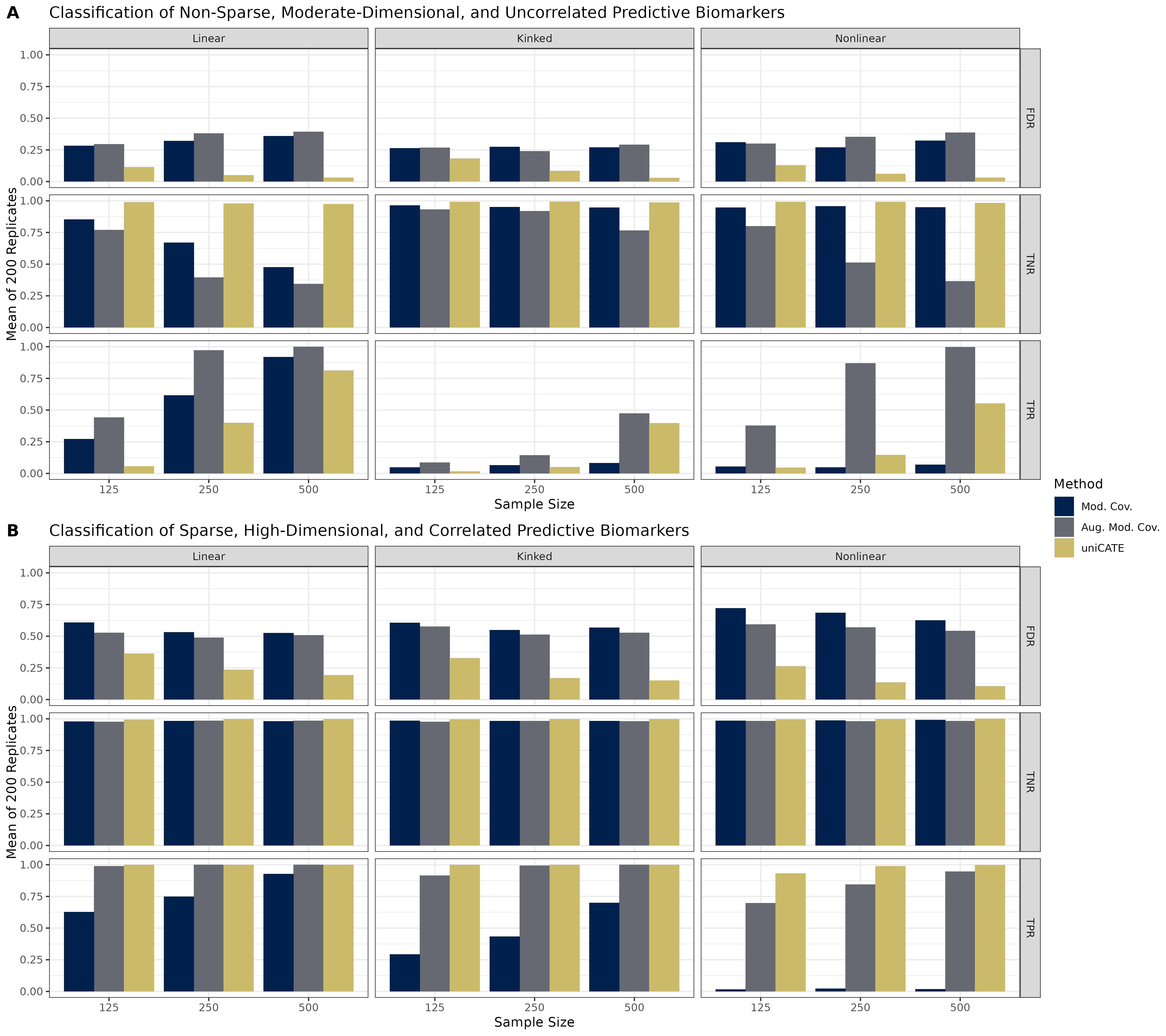
Our method’s capacity to identify predictive biomarkers was compared to that of popular CATE estimation methods: the modified covariates approach and its augmented counterpart (Tian et al. 2014; Chen et al. 2017). Briefly, the former directly estimates the linear model coefficients of the treatment-biomarker interactions, using a linear working model for these terms, without having to model or estimate the main effects. While Tian et al. 2014’s method is flexible since it avoids making any assumptions about the functional form of the main biomarker effects, it can lack precision in small-sample, high-dimensional settings. Tian et al. 2014 and Chen et al. 2017 therefore proposed “augmented” versions of this method that explicitly account for this source of variation. While Tian et al. 2014’s [Tian et al. 2014] and Chen et al. 2017’s [Chen et al. 2017] augmentation procedures differ, they are identical in the randomized control trials with continuous outcome variables (Chen et al. 2017): they are equivalent to fitting a (penalized) multivariate linear regression with treatment-biomarker interaction terms.
We again emphasize that these methods are not true competitors of our procedure. Their primary goal, CATE estimation, differs from that of uniCATE. However, Tian et al. 2014 and Chen et al. 2017 demonstrated that the (augmented) modified covariates approach could identify potentially predictive biomarkers when fit using regularized linear regressions like the LASSO. Biomarkers with non-zero treatment-biomarker interaction coefficient estimates are classified as predictive. We therefore applied these approaches, using 10-fold cross-validation to select the LASSO hyperparameters, to all simulated datasets. The implementations of these estimators provided by the personalized R software package (Huling and Yu 2021) was used.
The results pertaining to the moderate dimension simulations () with predictive biomarkers are presented in Figure 3A. Only uniCATE is capable of controlling the Type-I error rate; it approximately achieves the nominal FDR of 5% in all settings with samples sizes of 250 and above. The modified covariates approach and its augmented counterpart possess FDRs no lower than 25% across all scenarios. Indeed, their control of Type-I error generally worsens as sample size increases. Our method’s superior performance with respect to FDR control is likely due to its conservativeness: many of the predictive biomarkers are not recognized in smaller sample-size settings. As sample size grows, however, so too does its true positive rate (TPR) while maintaining a near perfect true negative rate (TNR). When , uniCATE generally identifies close to or more predictive biomarkers than the modified covariates approach, and nearly as many as the augmented modified covariates method.
Our procedure’s performance with respect to FDR control is again superior to that of the CATE estimation approaches in the high dimensional simulation scenarios with biomarkers (Figure 3B). While the adjustment procedure of Benjamini and Hochberg 1995 does not guarantee FDR control at the desired rate in these scenarios due to the correlation structure of the tests, it is nearly achieved in larger sample sizes. uniCATE also marginally outperforms other approaches in terms of the TNR. Unlike in the moderate sample-size simulations, however, our method identifies predictive biomarkers more efficiently than the other procedures considered.
These results demonstrate that uniCATE recovers truly predictive biomarkers more reliably than interpretable treatment rule estimators. In most simulation scenarios, uniCATE provides well controlled Type-I error rates while its TNR and TPR are comparable or superior to other methods. However, when the number of truly predictive biomarkers is large and the sample size small, uniCATE’s biomarker classification will be conservative. In this setting, our method still provides good Type-I error control, limiting the waste of resources on the investigation of false positives, as would be the result if using existing methods. If the investigator prefers a less conservative approach, since, for example, the cost of follow-up experiments is low, the (augmented) modified covariate approach may be considered instead.
5 Application to IMmotion Trials
Until recently, Tyrosine kinase inhibitors targeting vascular endothelial growth factor (VEGF) were the standard of care for patients with metastatic renal cell carcinoma (mRCC) (Rini et al. 2019). Unfortunately, many patients with mRCC find these treatments, like sunitinib, ineffective, and most develop a resistance over time (Rini and Atkins 2009). Immune checkpoint inhibitors like atezolizumab can produce more durable results and improve overall survival in pre-treated patients with mRCC (Motzer et al. 2015a; Motzer et al. 2015b; McDermott et al. 2018). A combination of atezolizumab and bevacizumab, the latter of which also binds to VEGF, was shown to improve the objective response rate (ORR) in a Phase 1b study (Wallin et al. 2016). Objective response is a binary indicator of clinically meaningful response to treatment. These findings were supported by a Phase 2 study, IMmotion 150, which compared atezolizumab alone and in combination with bevacizumab against sunitinib (McDermott et al. 2018). In a subsequent Phase 3 study, IMmotion 151 (Rini et al. 2019), the atezolizumab and bevacizumab combination improved progression free survival and objective response over sunitinib in patients whose cancer cells expressed the programmed death-1 ligand 1 (PD-L1), but not all of these patients showed benefit. These results motivate the search for biomarkers that are more predictive of this treatment’s clinical benefit than PD-L1 expression.
Potentially predictive biomarkers were found by applying uniCATE to subsets of the sunitinib () and atezolizumab-bevacizumab () treatment arms of the IMmotion 150 trial. Only patients with pre-treatment tumor RNA-seq samples were included. The 500 most variable genes based on this log-transformed RNA-seq data comprised the collection of potentially predictive biomarkers. Details of the gene expression data collection and preparation have previously been described by McDermott et al. 2018. Objective response was used as the outcome variable. The conditional outcome regression model was fit with a Super Learner whose library contained (penalized) GLMs with treatment-biomarker interaction terms, XGboost models, Random Forest models, and the mean model. A nominal FDR cutoff of 5% was employed. The modified covariates and augmented modified covariates approach for binary outcomes of Tian et al. 2014 were also applied to these data.
The uniCATE method identified 92 genes as predictive biomarkers, whereas the modified covariates approach and its augmented counterpart identified 20 and 6, respectively. All results are listed in Table S1. That the approaches of Tian et al. 2014 are more conservative than ours is a reversal of Section 4’s simulation results, but may be explained by the more complex correlation structure of these data. Indeed, the former rely on sparse linear models which are known to select but a few features from any given highly correlated set. Our procedure, however, uncovers sets of correlated predictive biomarkers since their individual hypothesis testing results will also be associated. This property is desirable when analyzing genomic data as large gene sets permit more thorough biological exploration and improved interpretation than do single, uncorrelated genes (Subramanian et al. 2005). The reporting of gene sets also improves the reproducibility of findings (Subramanian et al. 2005).
We performed a gene set enrichment analysis (GSEA) of gene ontology (GO) terms with uniCATE’s 92 predictive biomarkers using MSigDB (Subramanian et al. 2005; Liberzon et al. 2011). The top results are presented in Table S2. We found that these genes are generally associated with immune responses, including those mediated by B cells and lymphocytes. Similar findings have been reported by Au et al. 2021 in the context of clear cell renal cell carcinoma patients’ therapeutic responses to nivolumab, another immune checkpoint inhibitor.

Now, having learned of potentially predictive biomarkers, we assessed how well they delineate patient sub-populations in the IMmotion 151 study. This study’s subjects are believed to be drawn from the same population as those enrolled in IMmotion 150. Eight hundred and ten subjects possessed baseline tumor gene expression data for the 500 genes considered in our IMmotion 150 analysis: 406 in the atezolizumab-bevacizumab combination arm, and 404 in the sunitinib arm. Figure 4 presents the heatmaps of log-transformed gene expression data for each methods’ set of predictive genes. Subgroups are easily discerned in uniCATE’s heatmap, but not so much in the other procedures’. This further emphasizes the benefits of uniCATE’s capacity to identify sets of correlated predictive biomarkers. Note that the most prominent cluster of patients in the modified covariates method’s heatmap is driven by the XIST gene. It is not selected by the augmented modified covariates procedure or uniCATE. Upon further inspection, it does not appear to have a strong predictive effect (Figure S3).
It is unclear from these heatmaps alone whether these subgroups correspond to clusters of patients that benefit more from one therapy than another. We therefore established subgroups by performing hierarchical clustering with complete linkage using Euclidean distance on the methods’ selections of IMmotion 151’s log-transformed gene expression data. The difference in ORR was then computed between patients receiving the atezolizumab-bevacizumab combination and the sunitinib regiment within each of these subgroups. The subgroups identified by the (augmented) modified covariates methods’ biomarkers had negligible differences in ORR (not shown). Instead, we used their estimated treatment rules to predict whether each patient would benefit more from the atezolizumab-bevacizumab combination or sunitinib, and then computed the difference in ORR within these groups. The findings are presented in Figure 5.

Figure 5 evaluates the patient populations classified by each method. When classifying patients into subgroups, the modified covariates approach and the augmented modified covariates approach subset patients into two groups. Ideally, one of the patient groups should produce a large, positive ORR difference representing an increased benefit from the novel drug combination. Figure 5 shows that when two patient groups are of interest, uniCATE’s biomarkers-defined subgroups are comparable to the groups identified by the other two methods in terms of the effect size and the group size. The unsupervised clustering approach used in uniCATE also permits the definition of multiple clusters, providing a more refined investigation of patient sub-populations. When considering three or four clusters (), one subgroup is found to respond much better on average to the atezolizumab-bevacizumab combination than to sunitinib. This difference in ORR is greater than that of any subgroup defined using treatment assignment rules.
These results suggest that uniCATE uncovered biomarkers that influence whether mRCC patients are more likely to respond to tyrosyne kinase inhibitors alone or in combination with immune checkpoint inhibitors. More work is necessary to validate these findings, and to determine whether these biomarkers could form the basis of assays that inform treatment decisions. Demonstrating that these biomarkers are predictive of other clinical endpoints, like overall survival, progression-free survival and safety, would make for compelling evidence. Recovering these biomarkers in a comparison of this drug combination to the current standard of care would be more convincing still.
6 Discussion
In this work, we demonstrate how predictive biomarker discovery, typically a byproduct of treatment rule estimation, is better addressed as a standalone variable importance estimation problem. We derive a novel nonparametric estimator for a causal parameter which we argue is generally useful and interpretable, and show that this estimator is consistent and asymptotically linear under non-restrictive assumptions. We then verify that our proposed procedure’s asymptotic guarantees are approximately achieved across diverse data-generating distributions in a thorough simulation study of moderate to high-dimensional randomized control trials. Our method is then used in an exploratory analysis of real clinical trial data, producing biologically meaningful results that identify patient subgroups with greater treatment effect heterogeneity than procedures not explicitly developed for predictive biomarker discovery.
While we derive theory for uniCATE’s application to observational data, we benchmarked it exclusively in randomized control trial settings since they constitutes our primary application area of interest. Evaluating our method in quasi-experimental settings, however, offers an interesting avenue of future research. Subsequent work may also explore analogous (causal) variable importance parameters based on, for example, the relative CATE, or adapt the univariate CATE for time-to-event outcomes. The study of other non and semiparametric estimators of these parameters, such as one-step estimators or targeted maximum likelihood estimators, might also prove fruitful. Finally, future work might assess whether treatment effect variable importance parameter inference procedures could be coupled with novel multiple testing adjustment approaches, like that of Fithian and Lei 2020, to better account for the complex correlation structures often found among biomarkers.
Software
The uniCATE method is implemented in the open-source uniCATE R software package at github.com/insightsengineering/uniCATE. Internally, it relies on the cross-validated framework of the origami R package (Coyle and Hejazi 2018) and on Super Learning framework of the sl3 R package (Coyle et al. 2021). Version 0.1.0 of uniCATE was used to produce the results presented in Sections 4 and 5.
Reproducibility and Data Availability
Code to reproduce the simulation study of Section 4 and the analysis of Section 5 is available at github.com/PhilBoileau/pub_uniCATE.
The clinical trial data are available on the clinical study data request platform (https://vivli.org/). The IMmotion150 clinical data was from data cutoff date of Oct 17, 2016. The IMmotion151 clinical data was from data cutoff date of Dec 3, 2019. For overall response rate (ORR) calculation in both studies, a responder is defined as patients with their best confirmed overall response by investigator of Complete Response (CR) or Partial Response (PR) per RECIST v1.1, and non-responder otherwise.
The RNAseq data are available at: https://ega-archive.org/datasets/EGAD00001004183 and https://ega-archive.org/datasets/EGAD00001006618 The RNA-seq data was processed by removing patients with missing baseline samples, and were transferred to log10(CPM+1). In total of 22,997 genes were included whose median log10(CPM+1) is larger than 0.01.
Acknowledgement
PB gratefully acknowledges the support of the Fonds de recherche du Québec - Nature et technologies and the Natural Sciences and Engineering Research Council of Canada. The authors thank James Duncan and Dr. Nima Hejazi for helpful discussions about the methodology, and Dr. Romain Banchereau and Dr. Zoe Assaf for helpful discussions about the analysis presented in Section 5. The authors would also like to thank Molly He for preliminary simulation results that prompted this project. Conflicts of interest: none declared.
Appendix
S1 Proofs
Theorem 1: Identification and efficient influence function.
Proof.
Standard results ensure that is identified by : By the law of double expectation, we find that , and by A1, A2 that . We follow the general guidelines in the review of Hines et al. 2022b to derive the EIF of . Define the fixed distribution whose support is contained in the support of . We define the parametric submodel of for as
Then,
∎
Corollary 1: Estimating equation estimator derivation and double robustness.
Proof.
The estimating equation estimator for the biomarker is given by:
Then, by the Weak Law of Large Numbers,
If , then this estimator is consistent. The same is true if either or . ∎
Theorem 2: Limiting distribution of the estimating equation estimator.
Proof.
Define the plug-in estimator for the univariate CATE of biomarker with nuisance parameters estimate using as . Then we have through the von Mises expansion of about that
| (S1) |
The first term is the sum of mean-zero random variables, and so it converges to a Normal with variance equal to that of the EIF, scaled by , as . The second term is the bias term that is accounted for by the estimating equation estimator . The third and fourth terms are the empirical process and remainder terms, respectively, and we must show that they converge to zero in probability.
The analysis of empirical process term is identical to that of the average treatment effect presented in Zheng and van der Laan 2011 due to the similarity of these parameters. Essentially, so long as the conditional outcome regression and propensity score estimators converge in probability to some function under the L2 norm, the empirical process term is bounded in probability.
We now study the remainder term:
| (S2) |
If is known, as in a randomized control trial, then the remainder term is exactly zero. When neither or is now known, then the remainder term of Equation (S1) is under the conditions of A4. The conditions on convergence rates can be relaxed even further: The remainder term converges to zero in probability so long as the last line of Equation (S2) is . That is, we may obtain our desired result even if, say, converges at slower rate to than in probability so long as converges more quickly to .
∎
S2 Additional Simulation Results


S3 Supporting Results from Application to IMmotion Trials
| Method | Predictive Biomarkers |
|---|---|
| Modified Covariates | ADCY8, CDH17, COL6A6, CSMD3, CXCL5, EEF1A2, GJB6, GRIA4, H19, IGKV1-9, KLK4, MMP3, MUC17, PZP, TCHH, TEX15, TRIM63, VIL1, WFIKKN2, XIST |
| Augmented Modified Covariates | EEF1A2, IGKV1-9, MMP3, PZP, TEX15, TRIM63 |
| uniCATE | WFIKKN2, NMRK2, KLK1, TRIM63, IGKV1-9, HHATL, UCHL1, CLDN1, EEF1A2, C8A, KCNJ3, ITIH2, IGLV3-21, TCHH, ATP1A3, IGLL5, ENPP3, IGKV3-15, IGLC3, SAA1, TEX15, IGKV1-16, IGKV1-5, IGHG1, GRIN2A, IGHV2-5, SERPIND1, IGHV1-18, DEFB1, CYP2J2, IGHV1-24, CES3, IGKV3-11, IGLV1-40, IGHV1-2, SLC17A4, KLK4, MMP7, ANKRD36BP2, IGHV3-11, IGHV4-31, IGHV4-34, IGLV3-19, HAMP, CSMD3, PDZK1IP1, IGHG3, MUC17, ALPK2, IGLV2-14, FRAS1, DNAH11, IGHGP, SAA2, BMPER, IGLV1-47, MMP3, FOSB, HPD, SYT13, IGHV4-59, SLC38A5, IGHA1, CYP2C9, IGKC, IGLC2, PGF, IGHV3-21, H19, FCRL5, PVALB, IGHV3-74, SLC6A3, IGHV1-46, IGLV2-23, IGLV3-1, HBA1, IGLV1-44, IGKV3-20, IGKV4-1, LAMA1, IGHV3-48, IGHV5-51, IGHG2, HBA2, KNG1, IGKV1-27, IGHM, IGLV2-11, FGL1, CYP4F22, IGLV1-51 |
| Rank | Gene Set Name | Genes in Set (K) | Description | Genes in Overlap (k) | k/K | p-value | FDR q-value |
|---|---|---|---|---|---|---|---|
| 1 | GOCC_IMMUNOGLOBULIN_COMPLEX | 157 | A protein complex that in its canonical form is composed of two identical immunoglobulin heavy chains and two identical immunoglobulin light chains, held together by disulfide bonds and sometimes complexed with additional proteins. An immunoglobulin complex may be embedded in the plasma membrane or present in the extracellular space, in mucosal areas or other tissues, or circulating in the blood or lymph. [GOC:add, GOC:jl, ISBN:0781765196] | 37 | 0.24 | 0 | 0 |
| 2 | GOBP_HUMORAL_IMMUNE _RESPONSE_MEDIATED_BY _CIRCULATING_IMMUNOGLOBULIN | 149 | An immune response dependent upon secreted immunoglobulin. An example of this process is found in Mus musculus. [GO_REF:0000022, GOC:add, ISBN:0781735149] | 36 | 0.24 | 0 | 0 |
| 3 | GOBP_COMPLEMENT_ACTIVATION | 171 | Any process involved in the activation of any of the steps of the complement cascade, which allows for the direct killing of microbes, the disposal of immune complexes, and the regulation of other immune processes; the initial steps of complement activation involve one of three pathways, the classical pathway, the alternative pathway, and the lectin pathway, all of which lead to the terminal complement pathway. [GO_REF:0000022, GOC:add, ISBN:0781735149] | 36 | 0.21 | 0 | 0 |
| 4 | GOMF_ANTIGEN_BINDING | 158 | Interacting selectively and non-covalently with an antigen, any substance which is capable of inducing a specific immune response and of reacting with the products of that response, the specific antibody or specifically sensitized T-lymphocytes, or both. Binding may counteract the biological activity of the antigen. [GOC:jl, ISBN:0198506732, ISBN:0721662544] | 35 | 0.22 | 0 | 0 |
| 5 | GOBP_B_CELL_MEDIATED _IMMUNITY | 219 | Any process involved with the carrying out of an immune response by a B cell, through, for instance, the production of antibodies or cytokines, or antigen presentation to T cells. [GO_REF:0000022, GOC:add, ISBN:0781735149] | 36 | 0.16 | 0 | 0 |
| 6 | GOBP_HUMORAL_IMMUNE _RESPONSE | 373 | An immune response mediated through a body fluid. [GOC:hb, ISBN:0198506732] | 37 | 0.10 | 0 | 0 |
| 7 | GOBP_LYMPHOCYTE _MEDIATED_IMMUNITY | 351 | Any process involved in the carrying out of an immune response by a lymphocyte. [GO_REF:0000022, GOC:add, ISBN:0781735149] | 36 | 0.10 | 0 | 0 |
| 8 | GOBP_ADAPTIVE_IMMUNE _RESPONSE_BASED_ON _SOMATIC_RECOMBINATION _OF_IMMUNE_RECEPTORS _BUILT_FROM_IMMUNOGLOBULIN _SUPERFAMILY_DOMAINS | 358 | An immune response mediated by lymphocytes expressing specific receptors for antigen produced through a somatic diversification process that includes somatic recombination of germline gene segments encoding immunoglobulin superfamily domains. Recombined receptors for antigen encoded by immunoglobulin superfamily domains include T cell receptors and immunoglobulins (antibodies) produced by B cells. The first encounter with antigen elicits a primary immune response that is slow and not of great magnitude. T and B cells selected by antigen become activated and undergo clonal expansion. A fraction of antigen-reactive T and B cells become memory cells, whereas others differentiate into effector cells. The memory cells generated during the primary response enable a much faster and stronger secondary immune response upon subsequent exposures to the same antigen (immunological memory). An example of this is the adaptive immune response found in Mus musculus. [GOC:add, GOC:mtg_sensu, ISBN:0781735149, ISBN:1405196831] | 36 | 0.10 | 0 | 0 |
| 9 | GOBP_REGULATION_OF _COMPLEMENT_ACTIVATION | 114 | Any process that modulates the frequency, rate or extent of complement activation. [GOC:go_curators] | 27 | 0.24 | 0 | 0 |
| 10 | GOBP_PHAGOCYTOSIS | 374 | A vesicle-mediated transport process that results in the engulfment of external particulate material by phagocytes and their delivery to the lysosome. The particles are initially contained within phagocytic vacuoles (phagosomes), which then fuse with primary lysosomes to effect digestion of the particles. [ISBN:0198506732] | 35 | 0.09 | 0 | 0 |

References
- Kraus [2018] Virginia B. Kraus. Biomarkers as drug development tools: discovery, validation, qualification and use. Nature Reviews Rheumatology, 14(6):354–362, Jun 2018. ISSN 1759-4804. doi:10.1038/s41584-018-0005-9. URL https://doi.org/10.1038/s41584-018-0005-9.
- Ginsburg and Phillips [2018] Geoffrey S. Ginsburg and Kathryn A. Phillips. Precision medicine: From science to value. Health Affairs, 37(5):694–701, 2018. doi:10.1377/hlthaff.2017.1624. URL https://doi.org/10.1377/hlthaff.2017.1624. PMID: 29733705.
- Royston and Sauerbrei [2008] Patrick Royston and Willi Sauerbrei. Interactions between treatment and continuous covariates: A step toward individualizing therapy. Journal of Clinical Oncology, 26(9):1397–1399, 2008. doi:10.1200/JCO.2007.14.8981. URL https://doi.org/10.1200/JCO.2007.14.8981. PMID: 18349388.
- Robins et al. [2008] James Robins, Liliana Orellana, and Andrea Rotnitzky. Estimation and extrapolation of optimal treatment and testing strategies. Statistics in Medicine, 27(23):4678–4721, 2008. doi:https://doi.org/10.1002/sim.3301. URL https://onlinelibrary.wiley.com/doi/abs/10.1002/sim.3301.
- Tian et al. [2014] Lu Tian, Ash A. Alizadeh, Andrew J. Gentles, and Robert Tibshirani. A simple method for estimating interactions between a treatment and a large number of covariates. Journal of the American Statistical Association, 109(508):1517–1532, 2014. doi:10.1080/01621459.2014.951443. URL https://doi.org/10.1080/01621459.2014.951443. PMID: 25729117.
- Luedtke and van der Laan [2016] Alexander R. Luedtke and Mark J. van der Laan. Super-learning of an optimal dynamic treatment rule. The International Journal of Biostatistics, 12(1):305–332, 2016. doi:doi:10.1515/ijb-2015-0052. URL https://doi.org/10.1515/ijb-2015-0052.
- Chen et al. [2017] Shuai Chen, Lu Tian, Tianxi Cai, and Menggang Yu. A general statistical framework for subgroup identification and comparative treatment scoring. Biometrics, 73(4):1199–1209, 2017. doi:https://doi.org/10.1111/biom.12676. URL https://onlinelibrary.wiley.com/doi/abs/10.1111/biom.12676.
- Zhao et al. [2018] Qingyuan Zhao, Dylan S. Small, and Ashkan Ertefaie. Selective inference for effect modification via the lasso, 2018.
- Wager and Athey [2018] Stefan Wager and Susan Athey. Estimation and inference of heterogeneous treatment effects using random forests. Journal of the American Statistical Association, 113(523):1228–1242, 2018. doi:10.1080/01621459.2017.1319839. URL https://doi.org/10.1080/01621459.2017.1319839.
- Fan et al. [2020] Qingliang Fan, Yu-Chin Hsu, Robert P. Lieli, and Yichong Zhang. Estimation of conditional average treatment effects with high-dimensional data. Journal of Business & Economic Statistics, 0(0):1–15, 2020. doi:10.1080/07350015.2020.1811102. URL https://doi.org/10.1080/07350015.2020.1811102.
- Bahamyirou et al. [2022] Asma Bahamyirou, Mireille E. Schnitzer, Edward H. Kennedy, Lucie Blais, and Yi Yang. Doubly robust adaptive lasso for effect modifier discovery. The International Journal of Biostatistics, 2022. doi:doi:10.1515/ijb-2020-0073. URL https://doi.org/10.1515/ijb-2020-0073.
- Hines et al. [2022a] Oliver Hines, Karla Diaz-Ordaz, and Stijn Vansteelandt. Variable importance measures for heterogeneous causal effects, 2022a. URL https://arxiv.org/abs/2204.06030.
- Levy et al. [2021] Jonathan Levy, Mark van der Laan, Alan Hubbard, and Romain Pirracchio. A fundamental measure of treatment effect heterogeneity. Journal of Causal Inference, 9(1):83–108, 2021.
- Hastie et al. [2009] Trevor Hastie, Robert Tibshirani, and Jerome Friedman. The elements of statistical learning: Data mining, inference and prediction. Springer, 2 edition, 2009. URL http://www-stat.stanford.edu/˜tibs/ElemStatLearn/.
- Sechidis et al. [2018] Konstantinos Sechidis, Konstantinos Papangelou, Paul D Metcalfe, David Svensson, James Weatherall, and Gavin Brown. Distinguishing prognostic and predictive biomarkers: an information theoretic approach. Bioinformatics, 34(19):3365–3376, 05 2018. ISSN 1367-4803. doi:10.1093/bioinformatics/bty357. URL https://doi.org/10.1093/bioinformatics/bty357.
- Zhu et al. [2022] Wencan Zhu, Céline Lévy-Leduc, and Nils Ternès. Identification of prognostic and predictive biomarkers in high-dimensional data with pplasso, 2022. URL https://arxiv.org/abs/2202.01970.
- Hao and Zhang [2014] Ning Hao and Hao Helen Zhang. Interaction screening for ultrahigh-dimensional data. Journal of the American Statistical Association, 109(507):1285–1301, 2014. doi:10.1080/01621459.2014.881741. URL https://doi.org/10.1080/01621459.2014.881741. PMID: 25386043.
- Jiang and Liu [2014] Bo Jiang and Jun S. Liu. Variable selection for general index models via sliced inverse regression. The Annals of Statistics, 42(5), oct 2014. doi:10.1214/14-aos1233. URL https://doi.org/10.1214%2F14-aos1233.
- Tang et al. [2020] Cheng Yong Tang, Ethan X Fang, and Yuexiao Dong. High-dimensional interactions detection with sparse principal hessian matrix. J. Mach. Learn. Res., 21:19–1, 2020.
- Rubin [1974] D.B. Rubin. Estimating causal effects of treatments in randomized and nonrandomized studies. Journal of Educational Psychology, 66(5):688–701, 1974.
- Bickel et al. [1993] Peter J Bickel, Chris AJ Klaassen, YA’Acov Ritov, and Jon A Wellner. Efficient and adaptive estimation for semiparametric models. Johns Hopkins University Press Baltimore, 1993.
- Hines et al. [2022b] Oliver Hines, Oliver Dukes, Karla Diaz-Ordaz, and Stijn Vansteelandt. Demystifying statistical learning based on efficient influence functions. The American Statistician, 0(ja):1–48, 2022b. doi:10.1080/00031305.2021.2021984. URL https://doi.org/10.1080/00031305.2021.2021984.
- Pfanzagl and Wefelmeyer [1985] J Pfanzagl and W Wefelmeyer. Contributions to a general asymptotic statistical theory. Statistics & Risk Modeling, 3(3-4):379–388, 1985.
- van der Laan and Robins [2003] Mark J van der Laan and James M Robins. Unified Methods for Censored Longitudinal Data and Causality. Springer Science & Business Media, 2003.
- Chernozhukov et al. [2017] Victor Chernozhukov, Denis Chetverikov, Mert Demirer, Esther Duflo, Christian Hansen, and Whitney Newey. Double/debiased/neyman machine learning of treatment effects. American Economic Review, 107(5):261–65, May 2017. doi:10.1257/aer.p20171038. URL https://www.aeaweb.org/articles?id=10.1257/aer.p20171038.
- Chernozhukov et al. [2018] Victor Chernozhukov, Denis Chetverikov, Mert Demirer, Esther Duflo, Christian Hansen, Whitney Newey, and James Robins. Double/debiased machine learning for treatment and structural parameters. The Econometrics Journal, 21(1):C1–C68, 01 2018. ISSN 1368-4221. doi:10.1111/ectj.12097. URL https://doi.org/10.1111/ectj.12097.
- van der Laan and Rubin [2006] Mark J van der Laan and Daniel Rubin. Targeted maximum likelihood learning. The International Journal of Biostatistics, 2(1), 2006.
- van der Laan and Rose [2011] Mark J van der Laan and Sherri Rose. Targeted learning: causal inference for observational and experimental data. Springer Science & Business Media, 2011.
- van der Laan and Rose [2018] Mark J van der Laan and Sherri Rose. Targeted Learning in Data Science: Causal Inference for Complex Longitudinal Studies. Springer Science & Business Media, 2018.
- van der Laan et al. [2007] Mark J. van der Laan, Eric C Polley, and Alan E. Hubbard. Super learner. Statistical Applications in Genetics and Molecular Biology, 6(1), 2007. doi:doi:10.2202/1544-6115.1309. URL https://doi.org/10.2202/1544-6115.1309.
- van der Laan and Dudoit [2003] Mark J van der Laan and Sandrine Dudoit. Unified cross-validation methodology for selection among estimators and a general cross-validated adaptive epsilon-net estimator: Finite sample oracle inequalities and examples. Working Paper 130, University of California, Berkeley, Berkeley, 2003. URL https://biostats.bepress.com/ucbbiostat/paper130/.
- Farrell et al. [2021] Max H. Farrell, Tengyuan Liang, and Sanjog Misra. Deep neural networks for estimation and inference. Econometrica, 89(1):181–213, 2021. doi:https://doi.org/10.3982/ECTA16901. URL https://onlinelibrary.wiley.com/doi/abs/10.3982/ECTA16901.
- Hejazi et al. [2017] Nima S. Hejazi, Philippe Boileau, Mark J. van der Laan, and Alan E. Hubbard. A generalization of moderated statistics to data adaptive semiparametric estimation in high-dimensional biology, 2017. URL https://arxiv.org/abs/1710.05451.
- Watanabe et al. [2011] Toshiaki Watanabe, Takashi Kobunai, Yoko Yamamoto, Keiji Matsuda, Soichiro Ishihara, Keijiro Nozawa, Hisae Iinuma, Tsuyoshi Konishi, Hisanaga Horie, Hiroki Ikeuchi, Kiyoshi Eshima, and Tetsuichiro Muto. Gene expression signature and response to the use of leucovorin, fluorouracil and oxaliplatin in colorectal cancer patients. Clinical and Translational Oncology, 13(6):419–425, Jun 2011. ISSN 1699-3055. doi:10.1007/s12094-011-0676-z. URL https://doi.org/10.1007/s12094-011-0676-z.
- Boileau et al. [2021a] Philippe Boileau, Nima S. Hejazi, Mark J. van der Laan, and Sandrine Dudoit. Cross-validated loss-based covariance matrix estimator selection in high dimensions, 2021a. URL https://arxiv.org/abs/2102.09715.
- Boileau et al. [2021b] Philippe Boileau, Nima S. Hejazi, Brian Collica, Mark J. van der Laan, and Sandrine Dudoit. cvCovEst: Cross-validated covariance matrix estimator selection and evaluation in R. Journal of Open Source Software, 6(63):3273, 2021b. doi:10.21105/joss.03273. URL https://doi.org/10.21105/joss.03273.
- R Core Team [2022] R Core Team. R: A Language and Environment for Statistical Computing. R Foundation for Statistical Computing, Vienna, Austria, 2022. URL https://www.R-project.org/.
- Bickel and Levina [2008] Peter J. Bickel and Elizaveta Levina. Regularized estimation of large covariance matrices. The Annals of Statistics, 36(1):199 – 227, 2008. doi:10.1214/009053607000000758. URL https://doi.org/10.1214/009053607000000758.
- Cai et al. [2010] T. Tony Cai, Cun-Hui Zhang, and Harrison H. Zhou. Optimal rates of convergence for covariance matrix estimation. The Annals of Statistics, 38(4):2118 – 2144, 2010. doi:10.1214/09-AOS752. URL https://doi.org/10.1214/09-AOS752.
- Huber et al. [2015] Wolfgang Huber, Vincent J. Carey, Robert Gentleman, Simon Anders, Marc Carlson, Benilton S. Carvalho, Hector Corrada Bravo, Sean Davis, Laurent Gatto, Thomas Girke, Raphael Gottardo, Florian Hahne, Kasper D. Hansen, Rafael A. Irizarry, Michael Lawrence, Michael I. Love, James MacDonald, Valerie Obenchain, Andrzej K. Oleś, Hervé Pagès, Alejandro Reyes, Paul Shannon, Gordon K. Smyth, Dan Tenenbaum, Levi Waldron, and Martin Morgan. Orchestrating high-throughput genomic analysis with bioconductor. Nature Methods, 12(2):115–121, Feb 2015. ISSN 1548-7105. doi:10.1038/nmeth.3252. URL https://doi.org/10.1038/nmeth.3252.
- Parsana et al. [2021] Princy Parsana, Markus Riester, and Levi Waldron. curatedCRCData: Clinically Annotated Data for the Colorectal Cancer Transcriptome, 2021. This is a manually curated data collection for gene expression meta-analysis of patients with colorectal cancer. This resource provides uniformly prepared microarray data with curated and documented clinical metadata. It allows users to efficiently identify studies and patient subgroups of interest for analysis and to perform meta-analysis immediately without the challenges posed by harmonizing heterogeneous microarray technologies, study designs, expression data processing methods and clinical data formats.
- Ning et al. [2020] Yang Ning, Peng Sida, and Kosuke Imai. Robust estimation of causal effects via a high-dimensional covariate balancing propensity score. Biometrika, 107(3):533–554, 06 2020. ISSN 0006-3444. doi:10.1093/biomet/asaa020. URL https://doi.org/10.1093/biomet/asaa020.
- Tibshirani [1996] Robert Tibshirani. Regression shrinkage and selection via the lasso. Journal of the Royal Statistical Society. Series B (Methodological), 58(1):267–288, 1996. ISSN 00359246. URL http://www.jstor.org/stable/2346178.
- Zou and Hastie [2005] Hui Zou and Trevor Hastie. Regularization and variable selection via the elastic net. Journal of the Royal Statistical Society: Series B (Statistical Methodology), 67(2):301–320, 2005. doi:https://doi.org/10.1111/j.1467-9868.2005.00503.x. URL https://rss.onlinelibrary.wiley.com/doi/abs/10.1111/j.1467-9868.2005.00503.x.
- Stone et al. [1997] Charles J. Stone, Mark Hansen, Charles Kooperberg, and Young K. Truong. Polynomial splines and their tensor products in extended linear modeling. Ann. Statist, 25:1371–1470, 1997.
- Chen and Guestrin [2016] Tianqi Chen and Carlos Guestrin. XGBoost: A scalable tree boosting system. Proceedings of the 22nd ACM SIGKDD International Conference on Knowledge Discovery and Data Mining, pages 785–794, 2016. doi:10.1145/2939672.2939785. URL http://doi.acm.org/10.1145/2939672.2939785.
- Breiman [2001] Leo Breiman. Random forests. Machine Learning, 45(1):5–32, 2001. doi:10.1023/A:1010933404324. URL https://doi.org/10.1023/A:1010933404324.
- Benjamini and Hochberg [1995] Yoav Benjamini and Yosef Hochberg. Controlling the false discovery rate: A practical and powerful approach to multiple testing. Journal of the Royal Statistical Society. Series B (Methodological), 57(1):289–300, 1995. ISSN 00359246. URL http://www.jstor.org/stable/2346101.
- Huling and Yu [2021] Jared D. Huling and Menggang Yu. Subgroup identification using the personalized package. Journal of Statistical Software, 98(5):1–60, 2021. doi:10.18637/jss.v098.i05. URL https://www.jstatsoft.org/index.php/jss/article/view/v098i05.
- Rini et al. [2019] Brian I Rini, Thomas Powles, Michael B Atkins, Bernard Escudier, David F McDermott, Cristina Suarez, Sergio Bracarda, Walter M Stadler, Frede Donskov, Jae Lyun Lee, Robert Hawkins, Alain Ravaud, Boris Alekseev, Michael Staehler, Motohide Uemura, Ugo De Giorgi, Begoña Mellado, Camillo Porta, Bohuslav Melichar, Howard Gurney, Jens Bedke, Toni K Choueiri, Francis Parnis, Tarik Khaznadar, Alpa Thobhani, Shi Li, Elisabeth Piault-Louis, Gretchen Frantz, Mahrukh Huseni, Christina Schiff, Marjorie C Green, and Robert J Motzer. Atezolizumab plus bevacizumab versus sunitinib in patients with previously untreated metastatic renal cell carcinoma (immotion151): a multicentre, open-label, phase 3, randomised controlled trial. The Lancet, 393(10189):2404–2415, 2019. ISSN 0140-6736. doi:https://doi.org/10.1016/S0140-6736(19)30723-8. URL https://www.sciencedirect.com/science/article/pii/S0140673619307238.
- Rini and Atkins [2009] Brian I Rini and Michael B Atkins. Resistance to targeted therapy in renal-cell carcinoma. The Lancet Oncology, 10(10):992–1000, 2009. ISSN 1470-2045. doi:https://doi.org/10.1016/S1470-2045(09)70240-2. URL https://www.sciencedirect.com/science/article/pii/S1470204509702402.
- Motzer et al. [2015a] Robert J. Motzer, Bernard Escudier, David F. McDermott, Saby George, Hans J. Hammers, Sandhya Srinivas, Scott S. Tykodi, Jeffrey A. Sosman, Giuseppe Procopio, Elizabeth R. Plimack, Daniel Castellano, Toni K. Choueiri, Howard Gurney, Frede Donskov, Petri Bono, John Wagstaff, Thomas C. Gauler, Takeshi Ueda, Yoshihiko Tomita, Fabio A. Schutz, Christian Kollmannsberger, James Larkin, Alain Ravaud, Jason S. Simon, Li-An Xu, Ian M. Waxman, and Padmanee Sharma. Nivolumab versus everolimus in advanced renal-cell carcinoma. New England Journal of Medicine, 373(19):1803–1813, 2015a. doi:10.1056/NEJMoa1510665. URL https://doi.org/10.1056/NEJMoa1510665. PMID: 26406148.
- Motzer et al. [2015b] Robert J. Motzer, Brian I. Rini, David F. McDermott, Bruce G. Redman, Timothy M. Kuzel, Michael R. Harrison, Ulka N. Vaishampayan, Harry A. Drabkin, Saby George, Theodore F. Logan, Kim A. Margolin, Elizabeth R. Plimack, Alexandre M. Lambert, Ian M. Waxman, and Hans J. Hammers. Nivolumab for metastatic renal cell carcinoma: Results of a randomized phase ii trial. Journal of Clinical Oncology, 33(13):1430–1437, 2015b. doi:10.1200/JCO.2014.59.0703. URL https://doi.org/10.1200/JCO.2014.59.0703. PMID: 25452452.
- McDermott et al. [2018] David F. McDermott, Mahrukh A. Huseni, Michael B. Atkins, Robert J. Motzer, Brian I. Rini, Bernard Escudier, Lawrence Fong, Richard W. Joseph, Sumanta K. Pal, James A. Reeves, Mario Sznol, John Hainsworth, W. Kimryn Rathmell, Walter M. Stadler, Thomas Hutson, Martin E. Gore, Alain Ravaud, Sergio Bracarda, Cristina Suárez, Riccardo Danielli, Viktor Gruenwald, Toni K. Choueiri, Dorothee Nickles, Suchit Jhunjhunwala, Elisabeth Piault-Louis, Alpa Thobhani, Jiaheng Qiu, Daniel S. Chen, Priti S. Hegde, Christina Schiff, Gregg D. Fine, and Thomas Powles. Clinical activity and molecular correlates of response to atezolizumab alone or in combination with bevacizumab versus sunitinib in renal cell carcinoma. Nature Medicine, 24(6):749–757, 2018. doi:10.1038/s41591-018-0053-3. URL https://doi.org/10.1038/s41591-018-0053-3.
- Wallin et al. [2016] Jeffrey J. Wallin, Johanna C. Bendell, Roel Funke, Mario Sznol, Konstanty Korski, Suzanne Jones, Genevive Hernandez, James Mier, Xian He, F. Stephen Hodi, Mitchell Denker, Vincent Leveque, Marta Cañamero, Galina Babitski, Hartmut Koeppen, James Ziai, Neeraj Sharma, Fabien Gaire, Daniel S. Chen, Daniel Waterkamp, Priti S. Hegde, and David F. McDermott. Atezolizumab in combination with bevacizumab enhances antigen-specific t-cell migration in metastatic renal cell carcinoma. Nature Communications, 7(1):12624, 2016. doi:10.1038/ncomms12624. URL https://doi.org/10.1038/ncomms12624.
- Subramanian et al. [2005] Aravind Subramanian, Pablo Tamayo, Vamsi K. Mootha, Sayan Mukherjee, Benjamin L. Ebert, Michael A. Gillette, Amanda Paulovich, Scott L. Pomeroy, Todd R. Golub, Eric S. Lander, and Jill P. Mesirov. Gene set enrichment analysis: A knowledge-based approach for interpreting genome-wide expression profiles. Proceedings of the National Academy of Sciences, 102(43):15545–15550, 2005. ISSN 0027-8424. doi:10.1073/pnas.0506580102. URL https://www.pnas.org/content/102/43/15545.
- Liberzon et al. [2011] Arthur Liberzon, Aravind Subramanian, Reid Pinchback, Helga Thorvaldsdóttir, Pablo Tamayo, and Jill P. Mesirov. Molecular signatures database (MSigDB) 3.0. Bioinformatics, 27(12):1739–1740, 05 2011. ISSN 1367-4803. doi:10.1093/bioinformatics/btr260. URL https://doi.org/10.1093/bioinformatics/btr260.
- Au et al. [2021] Lewis Au, Emine Hatipoglu, Marc Robert de Massy, Kevin Litchfield, Gordon Beattie, Andrew Rowan, Desiree Schnidrig, Rachael Thompson, Fiona Byrne, Stuart Horswell, Nicos Fotiadis, Steve Hazell, David Nicol, Scott T.C. Shepherd, Annika Fendler, Robert Mason, Lyra Del Rosario, Kim Edmonds, Karla Lingard, Sarah Sarker, Mary Mangwende, Eleanor Carlyle, Jan Attig, Kroopa Joshi, Imran Uddin, Pablo D. Becker, Mariana Werner Sunderland, Ayse Akarca, Ignazio Puccio, William W. Yang, Tom Lund, Kim Dhillon, Marcos Duran Vasquez, Ehsan Ghorani, Hang Xu, Charlotte Spencer, José I. López, Anna Green, Ula Mahadeva, Elaine Borg, Miriam Mitchison, David A. Moore, Ian Proctor, Mary Falzon, Lisa Pickering, Andrew J.S. Furness, James L. Reading, Roberto Salgado, Teresa Marafioti, Mariam Jamal-Hanjani, Chris Abbosh, Kai-Keen Shiu, John Bridgewater, Daniel Hochhauser, Martin Forster, Siow-Ming Lee, Tanya Ahmad, Dionysis Papadatos-Pastos, Sam Janes, Peter Van Loo, Katey Enfield, Nicholas McGranahan, Ariana Huebner, Stephan Beck, Peter Parker, Henning Walczak, Tariq Enver, Rob Hynds, Ron Sinclair, Chi wah Lok, Zoe Rhodes, David Moore, Reena Khiroya, Giorgia Trevisan, Peter Ellery, Mark Linch, Sebastian Brandner, Crispin Hiley, Selvaraju Veeriah, Maryam Razaq, Heather Shaw, Gert Attard, Mita Afroza Akther, Cristina Naceur-Lombardelli, Lizi Manzano, Maise Al-Bakir, Simranpreet Summan, Nnenna Kanu, Sophie Ward, Uzma Asghar, Emilia Lim, Faye Gishen, Adrian Tookman, Paddy Stone, Caroline Stirling, Nikki Hunter, Sarah Vaughan, Mary Mangwende, Lavinia Spain, Haixi Yan, Ben Shum, Eleanor Carlyle, Nadia Yousaf, Sanjay Popat, Olivia Curtis, Gordon Stamp, Antonia Toncheva, Emma Nye, Aida Murra, Justine Korteweg, Debra Josephs, Ashish Chandra, James Spicer, Ruby Stewart, Lara-Rose Iredale, Tina Mackay, Ben Deakin, Debra Enting, Sarah Rudman, Sharmistha Ghosh, Lena Karapagniotou, Elias Pintus, Andrew Tutt, Sarah Howlett, Vasiliki Michalarea, James Brenton, Carlos Caldas, Rebecca Fitzgerald, Merche Jimenez-Linan, Elena Provenzano, Alison Cluroe, Grant Stewart, Colin Watts, Richard Gilbertson, Ultan McDermott, Simon Tavare, Emma Beddowes, Patricia Roxburgh, Andrew Biankin, Anthony Chalmers, Sioban Fraser, Karin Oien, Andrew Kidd, Kevin Blyth, Matt Krebs, Fiona Blackhall, Yvonne Summers, Caroline Dive, Richard Marais, Fabio Gomes, Mat Carter, Jo Dransfield, John Le Quesne, Dean Fennell, Jacqui Shaw, Babu Naidu, Shobhit Baijal, Bruce Tanchel, Gerald Langman, Andrew Robinson, Martin Collard, Peter Cockcroft, Charlotte Ferris, Hollie Bancroft, Amy Kerr, Gary Middleton, Joanne Webb, Salma Kadiri, Peter Colloby, Bernard Olisemeke, Rodelaine Wilson, Ian Tomlinson, Sanjay Jogai, Christian Ottensmeier, David Harrison, Massimo Loda, Adrienne Flanagan, Mairead McKenzie, Allan Hackshaw, Jonathan Ledermann, Kitty Chan, Abby Sharp, Laura Farrelly, Hayley Bridger, George Kassiotis, Benny Chain, James Larkin, Charles Swanton, Sergio A. Quezada, Samra Turajlic, Ben Challacombe, Ashish Chandra, Simon Chowdhury, William Drake, Archana Fernando, Karen Harrison-Phipps, Steve Hazell, Peter Hill, Catherine Horsfield, Tim O’Brien, Jonathon Olsburgh, Alexander Polson, Sarah Rudman, Mary Varia, and Hema Verma. Determinants of anti-pd-1 response and resistance in clear cell renal cell carcinoma. Cancer Cell, 39(11):1497–1518.e11, 2021. ISSN 1535-6108. doi:https://doi.org/10.1016/j.ccell.2021.10.001. URL https://www.sciencedirect.com/science/article/pii/S1535610821005432.
- Fithian and Lei [2020] William Fithian and Lihua Lei. Conditional calibration for false discovery rate control under dependence, 2020. URL https://arxiv.org/abs/2007.10438.
- Coyle and Hejazi [2018] Jeremy R. Coyle and Nima S. Hejazi. origami: A generalized framework for cross-validation in r. Journal of Open Source Software, 3(21):512, 2018. doi:10.21105/joss.00512. URL https://doi.org/10.21105/joss.00512.
- Coyle et al. [2021] Jeremy R Coyle, Nima S Hejazi, Ivana Malenica, and Oleg Sofrygin. sl3: Modern Pipelines for Machine Learning and Super Learning, 2021. URL https://doi.org/10.5281/zenodo.1342293. R package version 1.4.2.
- Zheng and van der Laan [2011] Wenjing Zheng and Mark J. van der Laan. Cross-Validated Targeted Minimum-Loss-Based Estimation, pages 459–474. Springer New York, New York, NY, 2011. ISBN 978-1-4419-9782-1. doi:10.1007/978-1-4419-9782-1_27. URL https://doi.org/10.1007/978-1-4419-9782-1_27.