Universal Optimality and Robust Utility Bounds for Metric Differential Privacy

Our contributions are as follows:

1. 1.

   Using principles from Quantitative Information Flow, we study optimality for metric differential privacy in full generality; that is, $\mathbf{d}$-private mechanisms which provide the best utility over arbitrary classes of loss functions. This extends the study by Ghosh et al. [4] and Brenner and Nissim [5] which considered optimality only for the central model and only for the class of monotonic loss functions.

2. 2.

   We provide a complete characterisation of optimality within a privacy type for finite ${\cal X}$. This characterisation is independent of the workflow (oblivious, local or otherwise) in which the privacy type arises. This result is significant in that it provides a finite class of mechanisms which characterise the space.

3. 3.

   We show that every privacy type contains universally optimal mechanisms (for non-trivial loss functions). This indicates that the impossibility result of Brenner and Nissim is too strong; we provide a tightening of their result, clarifying that the impossibility result for “sum queries” holds for a class of strictly monotonic consumers.

4. 4.

   We extend the qualitative study of optimality to a quantitative study, finding robust capacity bounds for universally optimal mechanisms within a privacy type. These capacity results provide a tight quantitative bound on the maximum leakage – a measure of the usefulness of a mechanism within a privacy type. In practice for example, such bounds provide benchmarks for experimental evaluation of implemented mechanisms.

The problem of universal optimality for arbitrary privacy types, as modelled by $\mathbf{d}$-privacy, has not yet been studied in full generality. Chatzikokolakis et al. [7] showed that optimal mechanisms for “sum queries” can be constructed in the oblivious setting by considering a Manhattan metric, rather than a Hamming metric, on the original datasets. Recent work by Fernandes et al. [10] considers universal optimality of the Laplace mechanism in the continuous setting, using the same QIF framework as in our paper, although our work focuses on a more general problem of universal optimality restricted to discrete spaces. Other optimality results have been found in non-Bayesian settings. Gupte et al. [11] proved a universal optimality result for a type of risk-averse consumer using a minimax formulation. Aharya et al. [12] prove an optimality result for binary mechanisms similar to our result of Cor. 9, but the focus of their work is on minimax consumers. Kairouz et al. [13] proved optimality for “staircase mechanisms” using $f$-divergence as a utility measure, while Koufogiannis et al. [14] showed that the Laplace mechanism is optimal for the mean-squared error. Finally, Asi and Duchi [15] studied near-instance optimality, designed for particular dataset instances, in contrast with our study of optimality over mechanisms. It is important to note that the notions of utility induced by the above non-Bayesian consumers are simpler than ours, and their trade-off with privacy is more direct. Also, the question of universality w.r.t. the prior does not arise. Furthermore, most of the results assume heavy restrictions on the noise functions.

We begin in §II with a summary of the results needed from Quantitative Information Flow including how to formulate the Universal optimality problem under the same assumption of “Bayesian consumers” as used by Ghosh et al. and Brenner and Nissim. In §III we introduce privacy types based on a metric $\mathbf{d}$ and a set of secrets $\mathcal{X}$; given these ingredients we provide a complete characterisation of the mechanisms of that type. In §IV we provide a thorough investigation of utility in terms of loss functions and how there is a close relationship between the complexity of the loss function and the structure of the underlying privacy mechanisms from which we can deduce both when universal properties exist and when they do not depending on the loss function (eg. its complexity) and the composition of the privacy mechanisms. In §V we introduce privacy type capacities and show that they provide a benchmark for computing how much useful information can be extracted from a privacy mechanism. Finally in §VI we provide a range of examples that illustrate these ideas.

Where possible we have sketched proofs in the main body of the paper. Full proofs can be found in the appendix.

QIF assumes that adversaries are Bayesian: they are equipped with a prior $\pi{:}\,\mathbb{D}{\mathcal{X}}$ over secrets $\mathcal{X}$ and use their knowledge of the channel $C{:}\,\mathcal{X}{\to}\mathbb{D}{\mathcal{Y}}$ to maximise their advantage after making an observation. This is modelled in full generality using the “$g$-leakage framework” [16]. In detail, a gain function $g{:}\,{\mathcal{W}{\times}\mathcal{X}}{\to}\mathbb{R}_{\geq 0}$ models the gain to an adversary who takes an action $w{\in}\mathcal{W}$ when the value of the secret is $x{\in}\mathcal{X}$. Focussing on actions rather than observations naturally encompasses the idea of “remapping” observations to their associated most likely secret value. Moreover $g$-leakage gives a measurement for how successful are (privacy) mechanisms at communicating useful information by comparing the “prior” and “posterior” $g$-vulnerabilities as follows. For gain function $g$ the (prior) vulnerability wrt. the prior $\pi$ (for a consumer/adversary with this information) is the maximum gain over all possible actions: $V_{g}(\pi){:=}\,\max_{w{{:}\,}\mathcal{W}}\sum_{x{{:}\,}\mathcal{X}}\pi_{x}g(w,x)$; it quantifies the adversary’s success in the scenario defined by $\pi$ and $g$. The expected (posterior) vulnerability is the adversary’s expected gain after observing $y$ is $V_{g}[\pi{\mathbin{\raisebox{1.00006pt}{\kern 0.50003pt\scriptsize$\vartriangleright$}}}C]{:=}\,\sum_{y{{:}\,}\mathcal{Y}}p(y)V_{g}(p(\mathcal{X}|y))$, equivalently:

The greater the difference in the prior/posterior vulnerability, the better is the adversary able to use the transmitted to infer the value of the secret. (See §II-B below.)

Note that we also use an equivalent formulation of leakage in terms of loss functions and minimising “generalised entropies”. In particular a function $\ell:\mathcal{W}{\times}\mathcal{X}\rightarrow\mathbb{R}$ (also) defines a generalised entropy $U_{\ell}:\mathbb{D}\mathcal{X}{\rightarrow}\mathbb{R}$:

with the formulation for expected loss through a channel defined similarly using minimisation (compare (3)):

We will often use $g$ for gain and $\ell$ for loss, but either can be used in formulating a vulnerability ($V_{g}/V_{\ell}$) or generalised entropy ($U_{g}/U_{\ell}$); the leakage theory based on losses or gains is equivalent [3].

Equation (3) indicates that the actual output $\mathcal{Y}$ can be abstracted, leaving the leakage properties of a channel in the context of a prior to be determined by a hyper-distribution (or simply “hyper”). A hyper is a distribution of distributions on $\mathcal{X}$, having type $\mathbb{D}\mathbb{D}{\mathcal{X}}$ or $\mathbb{D}^{2}{\mathcal{X}}$. Given a channel $C$ and prior $\pi$, we write $[\pi{\mathbin{\raisebox{1.00006pt}{\kern 0.50003pt\scriptsize$\vartriangleright$}}}C]$ for the hyper whose support is the set of posterior distributions $p(\mathcal{X}|y)$ on $\mathcal{X}$ and which assigns the corresponding marginal $p(y)$ to each. We usually denote by $\delta^{y}$ the posterior $p(\mathcal{X}|y)$ and by $\alpha_{y}$ its corresponding marginal.

An example of a channel and hyper is shown in Figure 1. The hyper $\Delta_{C}$ is produced by pushing the uniform prior through the channel $C$ to produce a joint distribution, which is then marginalised along its columns to produce the posteriors $\delta^{y}$ (the columns in $\Delta_{C}$) and the corresponding $y$-marginals $\alpha_{y}$ (the labels beneath each column). The prior $\pi$ can be recovered by averaging the posteriors $\delta_{y}$ via the marginals $\alpha_{y}$, revealing a significant correspondence between channels and hypers:

Figure 1 illustrates this relationship between a channel and its associated hyper.

It turns out that hypers, and their refinement relation, have a compelling geometric interpretation (first explained in [3, Ch. 12]), which we use below to study optimal utility.

The study of $g$-vulnerabilities has given rise to an elegant theory of refinement: we say that channel $A$ refines channel $B$, written $B\sqsubseteq A$, to mean that $A$ is safer than $B$ which holds exactly when the $g$-vulnerability of $A$ is no greater than that of $B$ for any prior or gain function, ie.,

The above holds dually for $U_{\ell}[\pi{\mathbin{\raisebox{1.00006pt}{\kern 0.50003pt\scriptsize$\vartriangleright$}}}A]\geq U_{\ell}[\pi{\mathbin{\raisebox{1.00006pt}{\kern 0.50003pt\scriptsize$\vartriangleright$}}}B]$. Remarkably, this holds whenever there exists a channel $P$ such that $BP=A$ (writing $BP$ for matrix multiplication) [17]. In fact $P$ corresponds to a “postprocessing” of the output of a channel, always suppressing information flow. The channel $\mathbb{I}$ with a single column of $1$’s is maximal in the refinement order, and leaks nothing at all i.e. $U_{\ell}[\pi{\mathbin{\raisebox{1.00006pt}{\kern 0.50003pt\scriptsize$\vartriangleright$}}}\mathbb{I}]=U_{\ell}(\pi)$.

Note that refinement is a strong universal utility property of channels (and therefore mechanisms modelled as channels). Refinement between two channels $A$ and $B$ means that for all priors and all gain (loss) functions channel $A$ will always have more gain (less loss) when compared to the corresponding scenario for channel $B$. We shall see therefore that when $A,B$ are members of the same privacy type then a refinement relation between them implies a universal optimality property between the two. We find, however, that in general there is no mechanism that anti-refines all mechanisms within the type, and therefore the universal optimality property can only hold for a subset of specific gain/loss functions.

Equivalently, refinement can be expressed as a relation between hypers: $[\pi{\mathbin{\raisebox{1.00006pt}{\kern 0.50003pt\scriptsize$\vartriangleright$}}}B]\sqsubseteq[\pi{\mathbin{\raisebox{1.00006pt}{\kern 0.50003pt\scriptsize$\vartriangleright$}}}A]$ exactly when there is a “refining Earth Move” (defined below) from the posteriors of $[\pi{\mathbin{\raisebox{1.00006pt}{\kern 0.50003pt\scriptsize$\vartriangleright$}}}B]$ to the posteriors of $[\pi{\mathbin{\raisebox{1.00006pt}{\kern 0.50003pt\scriptsize$\vartriangleright$}}}A]$. We recall the important correspondence between refinement of channels and refinement of hypers [3, Ch. 12]:

where $\pi$ is any full support prior. In other words, refinement of channels (on all priors) is characterised by refinement of hypers on a single (full support) prior.

In this paper we use this correspondence to characterise the space of $\mathbf{d}$-private mechanisms and those which are universally $\ell$-optimal. We write $\Delta$ etc. for general hypers on $\mathbb{D}^{2}{\mathcal{X}}$; we note that we can depict $\Delta$ as a weighted sum of vectors, where we identify each posterior $\delta^{y}$ in the support of $\Delta$ as a point in $\mathbb{R}^{|\mathcal{X}|}$. We make the following observations [3, Ch. 12]):

1. a)

   A “refining Earth Move” [18] from $\Delta_{B}$ to $\Delta_{A}$ exists when each posterior $\delta^{y}$ of $\Delta_{A}$ is realised as a convex combination of posteriors of $\Delta_{B}$ (ie. an “Earth Move” from $\Delta_{B}$ to each $\delta^{y}$) which exactly match the marginals of $\Delta_{B}$ to produce the corresponding marginals on $\Delta_{A}$.

2. b)

   If $\Delta_{B}$’s posteriors are linearly independent (as vectors), the Earth Move from a) exists whenever the posteriors of $\Delta_{A}$ lie inside the convex hull of the posteriors of $\Delta_{B}$.

3. c)

   The difference between the posterior and prior vulnerabilities gives a measure of the accuracy of the channel. The additive $g$-leakage is $|V_{g}[\pi]-V_{g}[\pi{\mathbin{\raisebox{1.00006pt}{\kern 0.50003pt\scriptsize$\vartriangleright$}}}A]|$, and the multiplicative $g$-leakage is $V_{g}[\pi{\mathbin{\raisebox{1.00006pt}{\kern 0.50003pt\scriptsize$\vartriangleright$}}}A]/V_{g}[\pi]$. The corresponding channel capacities take the maximal difference over all priors and $\underline{\mathbb{G}{\mathcal{X}}}$, the $0/1$-bounded vulnerabilities. ³³ 3 i.e. $0\leq V_{g}[\pi]\leq 1$ Specifically the multiplicative and additive capacities respectively are:

   $${\cal ML}^{\times}(C)~{:=}\,\max_{\pi,g}(V_{g}[\pi{\mathbin{\raisebox{1.00006pt}{\kern 0.50003pt\scriptsize$\vartriangleright$}}}C]/V_{g}[\pi])$$

   (8)

   and

   $${\cal ML}^{+}(C)~{:=}\,\max_{\pi,g}|V_{g}[\pi]-V_{g}[\pi{\mathbin{\raisebox{1.00006pt}{\kern 0.50003pt\scriptsize$\vartriangleright$}}}C]|~.$$

   (9)

   It is easy to see that $1{\leq}{\cal ML}^{\times}(C){\leq}|\mathcal{X}|$ and $0{\leq}{\cal ML}^{+}(C){\leq}1$. The larger either capacity, the more accurate the channel. For example, ${\cal ML}^{+}({\mathbb{I}})=0$, and ${\cal ML}^{\times}({\mathbb{I}})=1$ consistent with it transmitting no information at all. Capacities provide an alternative robust bound on the ability of any mechanism in a privacy type to deliver accurate information since it represents a tight upper bound on the maximum leakage of any channel in the type. We show how to compute capacities for the whole type either by proving a universal optimality result or using the characterisation given in §III below.

We shall show that irrespective of whether a type can support universal optimality results, the capacities are well-defined and there exist mechanisms that achieve the capacity. Such mechanisms represent the most efficient implementations that respect the privacy threshold whilst at the same time delivering the most information about the utility.

Given the equivalence between utility notions in the literature and the QIF notion of posterior $\ell$-uncertainty (Remark 1), there is then a natural connection between utility and refinement which extends to universal optimality. In its most general form, we define universal optimality as:

Using Eqn 6, this says that $M\in{\cal T}$ is universally optimal whenever $M^{\prime}\sqsubseteq M$ for all $M^{\prime}\in{\cal T}$. This definition appears to be too strong; indeed most mechanisms –even within the same privacy type– are not related by refinement [19]. Surprisingly, we find that there is a class ${\cal T}$ for which this strong notion of universal optimality holds (Cor. 9). However, we also find that this class is unique (Thm. 11) and universal optimality is too strong in general.

Therefore, following Ghosh et al. we study a weaker order defined by specific loss functions:

The universal optimality definition adopted by Ghosh et al. is, using Def. 3, universal $\ell$-optimality for all “monotone” loss functions $\ell$ (see Def. 6 ahead). We can think of Def. 3 as describing a type of restricted refinement which holds for all priors but only for loss functions $\ell\in{\mathcal{L}}$. This idea of refinement restricted to loss function classes has not to our knowledge been previously studied, and is the focus of §IV.

Following [20], we write a mechanism $M$ of privacy type ${\cal T}_{\mathcal{X},\mathbf{d}}$ as a channel $C{:}\,{\cal X}\to\mathbb{D}{\mathcal{Y}}$ satisfying $C_{x,y}\leq e^{\mathbf{d}(x,x^{\prime})}C_{x^{\prime},y}$ for all $x,x^{\prime}\in\mathcal{X}$ and $y\in\mathcal{Y}$. ie., As a set of constraints on each column of the channel. Importantly, there is a correspondence between $C$ and hyper-distributions as follows:

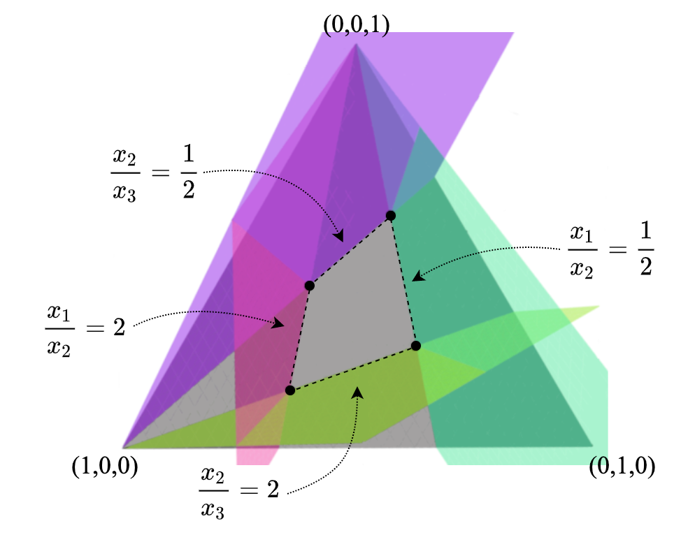
Applying Lem. 2 to each pair $x,x^{\prime}$ yields a feasible region of hypers (defined by their posteriors $\delta^{y}$) enclosed by hyperplanes –therefore convex– which we call “the space of ${\cal T}_{\mathcal{X},\mathbf{d}}$ hypers”. Figure 2 illustrates one such space.

Observe that although Lem. 2 specifies the uniform distribution, Eqn (7) says that this restriction does not apply to channel refinement. In other words, we can reason about channel refinement (over all priors) by reasoning in the space of hypers w.r.t. the uniform distribution. This differentiates our approach from standard convex optimisation formulations of the differential privacy constraints on channels [21] which require quantification over all priors.

The convex space above describes the complete set of potential posteriors which can be found in hyper-distributions $[\upsilon{\mathbin{\raisebox{1.00006pt}{\kern 0.50003pt\scriptsize$\vartriangleright$}}}C]$. Using Lem. 1, we can construct valid channels from a set of posteriors, provided that they contain the uniform distribution and can be averaged to the uniform prior. Moreover, Lem. 2 says that if the posteriors satisfy the $\mathbf{d}$-privacy constraints, then so will the corresponding channel. (Notice this in Figure 1: the ratio between elements in each column of $C$ matches the corresponding ratios in $\Delta_{C}$). This means we can construct $\mathbf{d}$-private channels from sets of $\mathbf{d}$-private posteriors. We use this fact now to examine optimality via hypers.

We distinguish 2 types of hypers (and their corresponding mechanisms) formed from vertices in the space of ${\cal T}_{\mathcal{X},\mathbf{d}}$ hypers:

Vertex mechanisms are of particular interest because of their refinement properties: they are the minimal elements in the refinement order in their privacy type (that is, they have no anti-refinements which satisfy the privacy constraints). Put another way, it means that every ${\cal T}_{\mathcal{X},\mathbf{d}}$ mechanism is a refinement of a vertex mechanism. (See Appendix §-B for details). However, (potentially) infinitely many exist in any privacy type. We will instead make use of particular vertex mechanisms that we call kernel mechanisms.

Importantly, every vertex mechanism can be expressed as a convex sum of kernel mechanisms, and these generate all ${\cal T}_{\mathcal{X},\mathbf{d}}$ mechanisms. This leads to the main result of this section.

The usefulness of this characterisation is that we can now explore questions about optimality using a finite set of kernel mechanisms as a basis for generating classes of universally optimal mechanisms.

Note that our notion of privacy types plays a role similar to that of “privacy constraint graph” in [5], but it is strictly more general. First of all, the “privacy (constraint) graph” is defined only for the central model, while, as explained in the introduction, the privacy types of $\mathbf{d}$-privacy subsume and generalise both the central and the local model. Furthermore, from a technical point of view, privacy graphs can be expressed using a metric, but the vice-versa is not true, since in privacy graphs there is no notion of distance between nodes.

A loss function defines a generalised entropy of type $\mathbb{D}{\cal X}\rightarrow\mathbb{R}$. Such entropies are concave (and continuous), i.e. $U_{\ell}(\pi_{1}+_{p}\pi_{2})\geq pU_{\ell}(\pi_{1})+(1{-}p)U_{\ell}(\pi_{2})$. There are many loss functions that have been identified as useful for analysing information flow properties, including accuracy of mechanisms.

Observe that the trivial loss functions are independent of the underlying metric and cannot be used to measure any non-trivial information flow property because they correspond to adversarial settings where the adversary does not have a choice of actions. The associated entropies of trivial loss functions, namely $U_{\ell}$ correspond to linear functions in $\mathbb{D}\mathcal{X}$, i.e. $U_{\ell}(p\times\pi_{1}+(1{-}p)\times\pi_{2})=p\times U_{\ell}(\pi_{1})+(1{-}p)\times U_{\ell}(\pi_{2})$, and in fact $U_{\ell}[\upsilon{\mathbin{\raisebox{1.00006pt}{\kern 0.50003pt\scriptsize$\vartriangleright$}}}M]=U_{\ell}[\upsilon]$ whatever the mechanism $M$. Non-trivial loss functions –corresponding to non-planar generalised entropies– are critical for measuring information flow properties as they characterise how much an adversary is able to use partial information leaks to further his intent. For example, $\ell_{\mathrm{nib}}$ (defined in Eqn (11)) can be seen to be non-trivial as depicted in Figure 3 at right: the planar regions represent the action taken by the adversary to minimise his loss relative to his (current) knowledge of the secret as represented by eg. a posterior distribution.

Ghosh et al. [4] were the first to identify some important structures in the relation between loss functions and privacy mechanisms. They identified the class of monotone loss functions relative to the privacy type ${\cal T}_{\mathbb{N},\mathbf{d}_{2}}$. In their formulation the function $\alpha$ acts as a “remapping” to select the most likely input for a given observation made as part of the privacy mechanism (here represented as a channel).

Finally we note that we shall see examples later that show that the consideration of whether a loss function is included in the monotone set is sensitive to the underlying metric.

The function $\ell_{\mathrm{bin}}$ is a loss function commonly used to measure the ability of an adversary to guess the secret: note that its corresponding entropy $U_{\ell_{\mathrm{bin}}}$ is referred to as Bayes’ Risk. Letting $\mathcal{W}=\mathcal{X}$, we define:

Its dual is defined

Observe that $\ell_{\mathrm{bin}}\in{\cal L}^{m}_{\mathbf{d}_{2}}$, but $\ell_{\mathrm{bin}}\not\in{\cal L}^{m^{+}}_{\mathbf{d}_{2}}$, whilst $\ell_{\mathrm{bin}}\in{\cal L}^{m^{+}}_{\mathbf{d}_{D}}$. Meanwhile $\ell_{\mathrm{nib}}$ is not monotone in any metric, but it is non-trivial and we shall see that it is significant for computing channel capacities.

When $\mathcal{W}$ and $\mathcal{X}$ are subsets of a Euclidean space, we can define an average loss function:

Note that $\ell_{\mathrm{Avg}}$ is strictly monotone in the type ${\cal T}_{{\mathbb{N}},\mathbf{d}_{2}}$; the corresponding entropy $U_{\ell_{\mathrm{Avg}}}$ computes the average distance from the true value of the secret.

Finally we also consider general non-monotone loss functions, where $\ell$ is an arbitrary real-valued loss function. Although these have not yet been studied for privacy mechanisms, they offer significant insights because they can express generic properties for studying property inferences [22, 3], and they can provide quantitative robustness measures due to the “miracle theorems” which quantify channel capacity. We recall these important results as follows.

Observe that Thm. 4 and Thm. 5 can give robust quantitative bounds on general information leakage properties (including utility) for privacy types discussed above. We will illustrate this for the Euclidean and Discrete metrics below.

One way to understand the $\ell$-optimality problem within a type is to make the association of the loss function with an adversary (or consumer as in Ghosh et al. [4]) explicit. Recall that the loss function formalises an adversary’s intent by describing the cost of taking action $w$ when the secret is $x$. This means that a loss function is actually universally optimal for mechanism $M$ exactly when the adversary (formalised by $\ell$) can best make use of the information leaked by $M$ compared with any other mechanism in the privacy type. These adversaries prefer $M$ over all other mechanisms in the privacy type, independent of their prior knowledge. Thus rather than starting with a loss function $\ell$ and asking whether it has an $\ell$-optimal mechanism, instead given a mechanism $M$ ask which adversaries (loss functions) would prefer $M$ over all others. We study that idea next.

Notice that $L^{{\cal T}_{\mathcal{X},\mathbf{d}}}_{M}$ is closed under addition and multiplication by a non-negative generalised scalar, where addition is defined:

and generalised scalar multiplication is defined for (non-negative) real-valued function $v$:

Observe also that $L^{{\cal T}_{\mathcal{X},\mathbf{d}}}_{M}$ always contains ${\cal L}^{\star}$ the set of “trivial” loss functions, and the utility set for the trivial mechanism that leaks no information at all consists only of trivial loss functions.

More interestingly it turns out that the structure of a privacy mechanism is reflected in the structure of the corresponding utility sets. There are two important constructors for mechanisms where we see this relationship clearly. The first is the external probabilistic choice: for channels $M,M^{\prime}\in{\cal T}_{\mathcal{X},\mathbf{d}}$ we write $M{{{}_{p}}\oplus}M^{\prime}$ as the mechanism obtained by applying $M$ with probability $p$ and $M^{\prime}$ with probability $(1{-}p)$. This yields a channel containing the columns of $M$ scaled by $p$ together with the columns of $M^{\prime}$ scaled by $(1{-}p)$, whose columns therefore clearly satisfy the same differentially private constraints as $M,M^{\prime}$ and so $M{{{}_{p}}\oplus}M^{\prime}\in{\cal T}_{\mathcal{X},\mathbf{d}}$.

The second is restriction of a mechanism in ${\cal T}_{\mathcal{X},\mathbf{d}}$ to one in ${\cal T}_{{\mathcal{X}}^{\prime},\mathbf{d}}$ where $\mathcal{X}^{\prime}\subset\mathcal{X}$. We write ${M}\!\!\downarrow\!\!{X^{\prime}}$ for the restriction of the mechanism $M\in{\cal T}_{\mathcal{X},\mathbf{d}}$ to operate only on the subset of secrets $X^{\prime}$ obtained by removing rows of $M$ corresponding to the secrets $\mathcal{X}-\mathcal{X}^{\prime}$. Notice that ${M}\!\!\downarrow\!\!{X^{\prime}}$ retains the original metric $\mathbf{d}$ because the differentially-private constraints are only evaluated on the rows corresponding to secrets in $X^{\prime}$.

Correspondingly in the space of loss functions we have the following constructions. Denote by ${\ell}\!\!\downarrow\!\!{X^{\prime}}$ the restriction of the loss function $\ell$ to some subset $X^{\prime}$ of its secrets, defined by $({\ell}\!\!\downarrow\!\!{X^{\prime}})(w,x){:=}\,\ell(w,x)$ for $x\in X^{\prime}$. Conversely we can lift a loss function to a superset of secrets $\mathcal{X}$, denoted ${\ell}\!\!\uparrow\!\!{\mathcal{X}}$; it is obtained by “padding” the loss function with 0’s. That is, $({\ell}\!\!\uparrow\!\!{\mathcal{X}})(w,x){:=}\,\ell(w,x)$ when $x\in X\subseteq\mathcal{X}$ and $0$ when $x\not\in X$.

We observe now that utility sets have a structure that is dual to the structure of mechanisms.

Notice that Thm. 6(1) means that $L^{{\cal T}_{\mathcal{X},\mathbf{d}}}_{M}$ is always non-empty, containing at least the set of trivial loss functions. As might be expected, Thm. 6(2) implies that the more information leaked through a mechanism, the more loss functions it has in its utility set, with Thm. 6(3) showing that the trivial mechanism, which always implements differential privacy (since it leaks no information at all), is only universally $\ell$-optimal for the set of trivial loss functions.

Next, Thm. 6(4) shows that when mechanisms are constructed using external probabilistic choice, the resulting utility set is the intersection of the utility sets of the components.

Finally, Thm. 6(5) provides an important method for discovering $\ell$-optimal results by studying simpler privacy types with fewer secrets, but having the same underlying metric. We make use of Thm. 6(5) in §VI when we find universal optimality results in various metric spaces of interest.

A corollary to Thm. 6 is that the kernel mechanisms generate maximal utility sets.

But even more, in cases where there is a unique kernel mechanism generating the privacy type, that mechanism satisfies “universal optimality”.

It turns out that there is exactly one space for which a unique kernel mechanism exists, and from Thm. 8 this yields the following universal optimality result:

The above result is significant in that it holds for all loss functions, and is non-trivial in the sense that binary mechanisms are of interest in the privacy community. (eg., the original Random Response mechanism of Warner which is used in Google’s RAPPOR [23]).

We shall see that using restriction and Thm. 6 we will be able to build non-trivial loss functions contained in the utility sets for kernel mechanisms for any privacy type.

As mentioned earlier, Brenner and Nissim [5] studied the question of universal $\ell$-optimality specifically for types described in terms of “privacy constraint graphs”, which for us can be described by using metrics. For example their “sum queries” can be considered as mechanisms in the privacy type ${\cal T}_{\mathcal{X},\mathbf{d}_{\textrm{D}}}$. Whilst their negative results apply only to $\ell_{\mathrm{bin}}$ within their characterisation of privacy types in terms of constraint graphs, they leave open the more fundamental question about whether optimality for non-trivial loss functions exists more generally. The next theorem (partially) answers that question, showing that non-trivial $\ell$-optimal mechanisms always exist even when $\mathbf{d}$ is the Discrete metric, and as a consequence universal $\ell$-optimality is more common than expected.

In particular Thm. 10 applies even when the underlying metric is $\mathbf{d}_{D}$. More significantly, once we have found basic non-trivial loss functions contained in a mechanisms utility set, we can construct more complex loss functions, also in the utility set, by using addition (Eqn (13)) and scaling (Eqn (14)). Moreover, depending on the underlying metric many kinds of loss function can be significant for evaluating accuracy. In fact $\ell_{\mathrm{bin}}$ and $\ell_{\mathrm{nib}}$ are particularly significant since, if a corresponding universally optimal mechanism exists within a type, a robust benchmark for optimal loss exists (see Thm. 15).

The universal impossibility results of Brenner and Nissim were studied for the monotone loss function class wrt “sum queries”. In this section we generalise this result to arbitrary metrics and loss functions. Importantly, we tighten the impossibility, showing that it holds only for the class of strictly monotone loss functions. We note that our proof is more general and direct than Brenner and Nissim’s result as we are able to access generic properties of the QIF framework.

We begin with a fundamental impossibility result:

Thm. 11 applies to all loss function classes, and thus is a strengthening of the Brenner and Nissim result in that it shows that the impossibility also applies to the “counting query” class of Ghosh et al.

In terms of the weaker universal $\ell$-optimality, Brenner and Nissim’s impossibility result for the Bayes’ risk loss function $\ell_{\mathrm{bin}}$ shows that, at least in the Discrete domain, there exist loss functions (and therefore consumers) for which no mechanisms are universally optimal. However, as we have seen, this is not the case for all loss functions, nor is it the case for all monotone loss functions. The next result tightens the impossibility for sum queries, showing that it holds for the class of strictly monotone loss functions.

Thm. 12 applies to many loss functions of interest. For example: the average loss function $\ell_{\mathrm{Avg}}$ is strictly monotone in $\mathbf{d}_{2}$ although it is non-monotone in $\mathbf{d}_{\textrm{D}}$; $\ell_{\mathrm{bin}}$ is strictly monotone in $\mathbf{d}_{\textrm{D}}$ but not strictly monotone in $\mathbf{d}_{2}$.

Curiously, Thm. 12 this depends on strictly monotone loss functions wrt any metric $\mathbf{d}$. To give some intuition about this result, the proof (detailed in Appendix §-C) shows that strict monotonicity (wrt any $\mathbf{d}$) implies that ${\ell}\!\!\downarrow\!\!{\{x_{1},x_{2}\}}$ is non-trivial for every $x_{1}\neq x_{2}$, and that Kernel mechanisms in the $\mathbf{d}_{\textrm{D}}$-privacy space always contain a pair $\{x_{1},x_{2}\}$ for which optimality only holds on trivial loss functions; viz. the result rests on the behaviour of ${\cal T}_{\mathcal{X},\mathbf{d}_{\textrm{D}}}$ mechanisms on 2 secrets.

This suggests that consumers who wish to differentiate over all pairs of secrets will not be well-served by mechanisms of the ${\cal T}_{\mathcal{X},\mathbf{d}_{\textrm{D}}}$ type. However, consumers who wish to distinguish between a particular pair of secrets can expect better utility, as optimal mechanisms exist in this case. (This follows from Thm. 10). This is really the nature of the discrete metric – it can distinguish between individual pairs of inputs, but not all pairs at the same time. This highlights the importance of understanding the metrics involved when designing mechanisms with the utility of consumers in mind.

Finally, the next corollary follows from the proof of Thm. 12 (detailed in Appendix §-C):

This is a strengthening of the result in [5] which proves the above for $\varepsilon$ over some threshold. Our result holds for all $\varepsilon$.

This privacy type is the one studied by Ghosh et al., corresponding to “counting queries”. Although rich with mechanisms, the Geometric mechanism is the only well-known of this type. It has two instances – the (infinite) Geometric mechanism with outputs over the whole of $\mathbb{Z}$ and the truncated Geometric mechanism, in which the output domain matches the input domain (typically a subsequence of $\mathbb{N}$). These instances in fact have the same leakage properties, ie., they are equivalent as channels and thus produce the same hyper-distribution [24].

Unsurprisingly (given its optimality properties), we find that the Geometric mechanism is a kernel mechanism.

Figure 4 depicts the space of ${\cal T}_{\mathbb{N},\mathbf{d}_{2}}$ mechanisms on 3 secrets. On $n$ inputs, this space is constructed from $2\times(n-1)$ linear DP constraints resulting in $2^{n-1}$ vertices – extreme points of the feasible region of posteriors of this type.

Table 4 lists all kernel mechanisms for $n$ up to 6.

Ghosh et al. showed that the Geometric mechanism is universally optimal for the class of monotone loss functions, meaning that it provides the most accuracy (within its type) to Bayesian consumers described by monotone loss functions. However this result does not provide any way to determine exactly how accurate the data release can be, even for this optimal mechanism. A QIF analysis is able to give robust measurements for the amount of leakage as expressed by gain or loss functions; combined with Thm. 15 we are now able to give robust measurements for the whole privacy class. In particular since ${\ell_{\mathrm{bin}}}\in L_{G}$, we deduce that the multiplicative channel capacity of the Geometric dominates the multiplicative channel capacity for any mechanism in the whole privacy type. Going further we can compute the exact dominating channel capacity. (Refer to Table 4 for numerical examples.)

We also observe that the Geometric mechanism is the kernel mechanism which obtains the additive capacity for the mechanisms we computed (cf. Table 4), suggesting that it may also be optimal for the non-monotone $\ell_{\mathrm{nib}}$ loss function.

This privacy type is the one studied by Brenner and Nissim, corresponding to “sum queries”. For an input space $\mathcal{X}$ of size $n$, the vertices of the convex region are points of intersection of $n-1$ hyperplanes, corresponding to $n-1$ distinct privacy constraints. Since there are only 2 possible distances under the discrete metric, each vertex can only contain 2 possible values, and so the number of possible vertices is given by $\sum_{i=1}^{n-1}\binom{n}{i}=2^{n}-2$.⁵⁵ 5 Thinking of each vertex as having either the ‘high’ or the ‘low’ value, this is the number of combinations for each choice of ‘high’ values. We present some of these mechanisms in Table 5, including the well-known “Random Response” mechanism.

We note that the Random Response mechanism is a kernel mechanism. The space of mechanisms on 3 secrets for the Discrete metric is depicted in Figure 5.

Brenner and Nissim studied mechanisms of this privacy type, focussing on Bayesian consumers and $\ell_{\mathrm{bin}}$, showing that no mechanism is universally optimal for $\ell_{\mathrm{bin}}$. Their result demonstrates that there is no mechanism for the Discrete privacy type with the same universal optimality properties as the Geometric mechanism in the Euclidean privacy type. However Thm. 10 indicates that there are in fact mechanisms which are $\ell$-optimal for some non-trivial (monotone) loss functions. The next example of a mechanism (also described by Brenner and Nissim) is in fact $\ell$-optimal for a non-trivial monotone loss function. Consider the following hypers of type ${\cal T}_{\mathcal{X},{\ln 2}{\cdot}\mathbf{d}_{\textrm{D}}}$ on $n$ inputs:

We use Thm. 6(5) as follows. Concentrating on inputs $X^{\dagger}{:=}\,\{x_{1},x_{n}\}$, we see that ${K_{A}}\!\!\downarrow\!\!{X^{\dagger}}{=}{K_{B}}\!\!\downarrow\!\!{X^{\dagger}}{=}T$ (where $T$ is the universally optimal mechanism from Cor. 9). Since $T$ is the unique Kernel mechanism in a 2-element state space, we have that both are $\ell_{e}$-optimal for loss function $\ell_{e}(w,x)$ which has two actions, labelled by $X^{\dagger}$, and is $0$ whenever $w\neq x$, and $1$ if $w=x$. ⁶⁶ 6 In fact both ${K_{A}}\!\!\downarrow\!\!{X^{\dagger}},{K_{B}}\!\!\downarrow\!\!{X^{\dagger}}$ are $\ell$-optimal for all loss functions on $X^{\dagger}$. From Figure 3 we can see immediately that $\ell_{e}$ is non-trivial, thus by Thm. 6(5) we see that both $K_{A},K_{B}$ are ${\ell_{e}}\!\!\uparrow\!\!{\mathcal{X}}$-optimal, as well as all probabilistic combinations $K_{A}\oplus_{p}K_{B}$ defined above.

While we can compute a capacity for the whole Euclidean type from the universal optimality of the Geometric, this is not possible on the Discrete space owing to the impossibility results for $\ell_{\mathrm{bin}}$. We can use instead the characterisation of its structure directly to compute dominating additive and multiplicative capacities giving a tight quantitative upper bound for the accuracy of any mechanisms in the type. The dominating multiplicative capacity is given by the random response $R$, and the dominating additive capacity is given by its dual $R^{\circ}$ as follows. Let $\varepsilon=-\ln\alpha=\ln\beta$ , and $k=1+(|\mathcal{X}|-1)e^{-\varepsilon}$ and $m=1+(|\mathcal{X}|-1)e^{\varepsilon}$, then:

The dual $R^{\circ}$ has the minimum elements on the diagonal whereas the Random Response $R$ has its maxima there. (Recall Figure 5 for illustration.)

References

- [1] C. Dwork, F. Mcsherry, K. Nissim, and A. Smith, “Calibrating noise to sensitivity in private data analysis,” in In Proceedings of the Third Theory of Cryptography Conference (TCC), ser. Lecture Notes in Computer Science, S. Halevi and T. Rabin, Eds., vol. 3876. Springer, 2006, pp. 265–284.
- [2] C. Dwork, “Differential privacy,” in 33rd International Colloquium on Automata, Languages and Programming (ICALP 2006), ser. Lecture Notes in Computer Science, M. Bugliesi, B. Preneel, V. Sassone, and I. Wegener, Eds., vol. 4052. Springer, 2006, pp. 1–12. [Online]. Available: http://dx.doi.org/10.1007/11787006_1
- [3] M. S. Alvim, K. Chatzikokolakis, A. McIver, C. Morgan, C. Palamidessi, and G. Smith, “The science of quantitative information flow,” 2019.
- [4] A. Ghosh, T. Roughgarden, and M. Sundararajan, “Universally utility-maximizing privacy mechanisms,” SIAM Journal on Computing, vol. 41, no. 6, pp. 1673–1693, 2012.
- [5] H. Brenner and K. Nissim, “Impossibility of differentially private universally optimal mechanisms,” in 2010 IEEE 51st Annual Symposium on Foundations of Computer Science. IEEE, 2010, pp. 71–80.
- [6] J. C. Duchi, M. I. Jordan, and M. J. Wainwright, “Local privacy and statistical minimax rates,” in Proceedings of the 54th Annual IEEE Symposium on Foundations of Computer Science (FOCS). IEEE Computer Society, 2013, pp. 429–438. [Online]. Available: https://doi.org/10.1109/FOCS.2013.53
- [7] K. Chatzikokolakis, M. E. Andrés, N. E. Bordenabe, and C. Palamidessi, “Broadening the scope of differential privacy using metrics,” in International Symposium on Privacy Enhancing Technologies Symposium. Springer, 2013, pp. 82–102.
- [8] M. E. Andrés, N. E. Bordenabe, K. Chatzikokolakis, and C. Palamidessi, “Geo-indistinguishability: Differential privacy for location-based systems,” in Proceedings of the 2013 ACM SIGSAC conference on Computer & communications security, 2013, pp. 901–914.
- [9] N. Fernandes, M. Dras, and A. McIver, “Generalised differential privacy for text document processing,” in Principles of Security and Trust - 8th International Conference, POST 2019, Held as Part of the European Joint Conferences on Theory and Practice of Software, ETAPS 2019, Prague, Czech Republic, April 6-11, 2019, Proceedings, 2019, pp. 123–148. [Online]. Available: https://doi.org/10.1007/978-3-030-17138-4_6
- [10] N. Fernandes, A. McIver, and C. Morgan, “The laplace mechanism has optimal utility for differential privacy over continuous queries,” in 36th Annual ACM/IEEE Symposium on Logic in Computer Science, LICS 2021, Rome, Italy, June 29 - July 2, 2021. IEEE, 2021, pp. 1–12. [Online]. Available: https://doi.org/10.1109/LICS52264.2021.9470718
- [11] M. Gupte and M. Sundararajan, “Universally optimal privacy mechanisms for minimax agents,” in Proceedings of the twenty-ninth ACM SIGMOD-SIGACT-SIGART symposium on Principles of database systems, 2010, pp. 135–146.
- [12] J. Acharya, K. Bonawitz, P. Kairouz, D. Ramage, and Z. Sun, “Context aware local differential privacy,” in International Conference on Machine Learning. PMLR, 2020, pp. 52–62.
- [13] P. Kairouz, S. Oh, and P. Viswanath, “Extremal mechanisms for local differential privacy,” The Journal of Machine Learning Research, vol. 17, no. 1, pp. 492–542, 2016.
- [14] F. Koufogiannis, S. Han, and G. J. Pappas, “Optimality of the laplace mechanism in differential privacy,” arXiv preprint arXiv:1504.00065, 2015.
- [15] H. A. J. C. Duchi, “Near instance-optimality in differential privacy,” 2020, arXiv:2005.10630v1, 2020.
- [16] M. S. Alvim, K. Chatzikokolakis, C. Palamidessi, and G. Smith, “Measuring information leakage using generalized gain functions,” in 2012 IEEE 25th Computer Security Foundations Symposium. IEEE, 2012, pp. 265–279.
- [17] A. McIver, C. Morgan, G. Smith, B. Espinoza, and L. Meinicke, “Abstract channels and their robust information-leakage ordering,” in Principles of Security and Trust - Third International Conference, POST 2014, Held as Part of the European Joint Conferences on Theory and Practice of Software, ETAPS 2014, Grenoble, France, April 5-13, 2014, Proceedings, ser. Lecture Notes in Computer Science, M. Abadi and S. Kremer, Eds., vol. 8414. Springer, 2014, pp. 83–102.
- [18] S. T. Rachev and L. Rüschendorf, Mass Transportation Problems: Volume I: Theory. Springer Science & Business Media, 1998, vol. 1.
- [19] K. Chatzikokolakis, N. Fernandes, and C. Palamidessi, “Comparing systems: Max-case refinement orders and application to differential privacy,” in Proc. CSF. IEEE Press, 2019.
- [20] M. S. Alvim, M. E. Andrés, K. Chatzikokolakis, and C. Palamidessi, “On the relation between differential privacy and quantitative information flow,” in Automata, Languages and Programming - 38th International Colloquium, ICALP 2011, Zurich, Switzerland, July 4-8, 2011, Proceedings, Part II, 2011, pp. 60–76. [Online]. Available: https://doi.org/10.1007/978-3-642-22012-8_4
- [21] N. E. Bordenabe, K. Chatzikokolakis, and C. Palamidessi, “Optimal geo-indistinguishable mechanisms for location privacy,” in Proc. CCS, 2014, pp. 251–262.
- [22] M. S. Alvim, N. Fernandes, A. McIver, and G. H. Nunes, “On privacy and accuracy in data releases (invited paper),” in 31st International Conference on Concurrency Theory, CONCUR 2020, September 1-4, 2020, Vienna, Austria (Virtual Conference), ser. LIPIcs, I. Konnov and L. Kovács, Eds., vol. 171. Schloss Dagstuhl - Leibniz-Zentrum für Informatik, 2020, pp. 1:1–1:18. [Online]. Available: https://doi.org/10.4230/LIPIcs.CONCUR.2020.1
- [23] Úlfar Erlingsson, V. Pihur, and A. Korolova, “RAPPOR: Randomized aggregatable privacy-preserving ordinal response,” in Proc. CCS, 2014, pp. 1054–1067.
- [24] K. Chatzikokolakis, N. Fernandes, and C. Palamidessi, “Refinement orders for quantitative information flow and differential privacy,” Journal of Cybersecurity and Privacy, vol. 1, no. 1, pp. 40–77, 2021.
-A Results supporting §II
The following shows the equivalence between the formulation of utility loss in the literature ([4, 5]) and the QIF formulation of posterior uncertainty.
Lemma 1.
Note that in the second-last step we employ a mapping from remaps to guesses . We can think of this as simply a relabelling of observations to guesses , and we can always ‘duplicate’ guesses so that there is a one-one correspondence between guesses and inputs.
-B Results supporting §III
The following establishes the correspondence between -private mechanisms and hyper-distributions.
See 2
Proof:
Recall that is -private whenever . Now rewrite as and the result follows. ∎
We next set out some key properties of kernel mechanisms which allow us to establish the fundamental characterisation. The first property tells us that kernel mechanisms are irreducible.
Property 1.
If is a kernel mechanism then there is no kernel mechanism st. where are hypers corresponding to mechanisms respectively.
Assume that is a kernel mechanism and (treating as sets of posteriors). Then the posteriors of must be linearly independent (from Def. 5). Therefore the uniform distribution can be uniquely expressed as a linear combination of posteriors of . ie. We can write for scalars and posteriors . But the same is true for . ie. Its posteriors are linearly independent and there is a unique combination that produces the uniform distribution. ie. We write . But the posteriors of . Therefore we can write