跳到论文正文
W Papers独立论文阅读器 arXiv:2205.00461 论文正文 计算阅读时间 · 0%
引用这篇论文根据当前论文元数据生成,正式投稿前建议核对。


License: arXiv.org perpetual non-exclusive license
arXiv:2205.00461v1 [math.AP] 01 May 2022

A Łojasiewicz Inequality in Hypocomplex Structures of ℝ2\mathbb{R}^{2}.

Abdelhamid Meziani Address: Department of Mathematics, Florida International University, Miami, FL, 33199, USA Email address: meziani@fiu.edu
Abstract.

For a real analytic complex vector field LL, in an open set of ℝ2\mathbb{R}^{2}, with local first integrals that are open maps, we attach a number μ≥1\mu\geq 1 (obtained through Łojasiewicz inequalities) and show that the equation L​u=fLu=f has bounded solution when f∈Lpf\in L^{p} with p>1+μp>1+\mu. We also establish a similarity principle between the bounded solutions of the equation L​u=A​u+B​u¯Lu=Au+B\overline{u} (with A,B∈LpA,B\in L^{p}) and holomorphic functions.

Key words and phrases: 
Łojasiewicz Inequality, Hypocomplex, Solvability, Vector field
2020 Mathematics Subject Classification
Primary 35C15; Secondary 35F05

1. Introduction

This paper deals with the solvability of real analytic complex vector fields defined in an open set 𝒪⊂ℝ2\mathcal{O}\subset\mathbb{R}^{2}. We assume that the vector field LL has local first integrals that are open maps everywhere. This implies the existence of a global first integral ZZ in 𝒪\mathcal{O} and allows us to take LL as L=Zx∂y−Zy∂xL=Z_{x}\partial_{y}-Z_{y}\partial_{x}. We associate to LL a number μ≥1\mu\geq 1 (in fact μ>1\mu>1 unless LL is elliptic everywhere). This number is derived from Łojasiewicz inequalities for first integrals. We use a generalized Cauchy operator

TZ​f​(x,y)=−1π​∫Ωf⁡(ξ,η)​𝒦(x,y)​(ξ,η)​𝑑ξ​𝑑η=−1π​∫Ωf⁡(ξ,η)​d​ξ​d​ηZ⁡(ξ,η)−Z⁡(x,y)T_{Z}f(x,y)=\frac{-1}{\pi}\int_{\Omega}f(\xi,\eta)\mathcal{K}_{(x,y)}(\xi,\eta)\,d\xi d\eta=\frac{-1}{\pi}\int_{\Omega}\frac{f(\xi,\eta)\,d\xi d\eta}{Z(\xi,\eta)-Z(x,y)}

to prove that for every f∈Lp​(Ω)f\in L^{p}(\Omega), with p>1+μp>1+\mu, we have u=TZ​f∈L∞​(Ω)u=T_{Z}f\,\in L^{\infty}(\Omega) and satisfies the equation L​u=fLu=f. We also prove a similarity between L∞L^{\infty}-solution of the equation L​u=A​u+B​u¯Lu=Au+B\overline{u}, where A,B∈Lp​(Ω)A,B\in L^{p}(\Omega), and the holomorphic functions HH defined in Z⁡(Ω)Z(\Omega). More precisely the solution uu can be written as u=H⁡(Z)​esu=H(Z)\mathrm{e}^{s} with HH holomorphic in Z⁡(Ω)Z(\Omega) and s∈L∞​(Ω)s\in L^{\infty}(\Omega).

The questions addressed in this paper are related to those contained in papers: [1], [3], [4], [5], [6], [9], [10], [11], [12], [14], [15], [16], [17], [18], [19], [20], [23] and others.

The organization of this paper is as follows. Section 2 deals with the necessary background and terminology. In section 3 we derive normal forms for first integrals that will be used in section 4 to introduce a Łojasiewicz number μ\mu for the vector field. In section 5, we show that for 1<q<1+1μ\displaystyle 1<q<1+\frac{1}{\mu}, the generalized Cauchy kernel 𝒦(x,y)​(ξ,η)\mathcal{K}_{(x,y)}(\xi,\eta) satisfies ‖𝒦(x,y)‖Lq​(Ω)≤C\left\lVert\mathcal{K}_{(x,y)}\right\rVert_{L^{q}(\Omega)}\leq C for all (x,y)∈𝒪(x,y)\in\mathcal{O} where CC is a positive constant depending on Ω\Omega, qq and μ\mu. In section 6, we construct bounded solution of the equation L​u=fLu=f for f∈Lp​(Ω)f\in L^{p}(\Omega), with p>1+μp>1+\mu, and establish a similarity principle.

2. Preliminaries

In this section we set the necessary background and terminology used in the study of Hypoanalytic structures (see [4] and [23]). Let 𝒪⊂ℝ2\mathcal{O}\subset\mathbb{R}^{2} be open and connected and let

(2.1) L=A⁡(x,y)​∂∂x+B⁡(x,y)​∂∂yL=A(x,y)\displaystyle\frac{\partial}{\partial x}+B(x,y)\displaystyle\frac{\partial}{\partial y}

with A,B∈Cϖ​(𝒪,ℂ)A,B\,\in\,C^{\varpi}(\mathcal{O};\mathbb{C}) (A,BA,\,B real analytic and ℂ\mathbb{C}-valued in 𝒪\mathcal{O}). We assume that LL has no singular points: |A|+|B|>0|A|+|B|>0 everywhere in 𝒪\mathcal{O}. The conjugate of L¯\overline{L} is the vector field A¯∂x+B¯∂y\overline{A}\partial_{x}+\overline{B}\partial_{y}, where A¯\overline{A} and B¯\overline{B} are the complex conjugates of AA and BB. The vector field LL is elliptic at all points where LL and L¯\overline{L} are independent. At each elliptic point, LL is locally conjugate to the CR operator ∂∂z¯\displaystyle\displaystyle\frac{\partial}{\partial\overline{z}}. Denote by Σ\Sigma the set of non elliptic points. Thus Σ\Sigma is the real analytic variety given by

(2.2) Σ={(x,y)∈𝒪:Im​(A⁡(x,y)​B⁡(x,y)¯)=0}.\Sigma=\left\{(x,y)\in\mathcal{O}:\ \textrm{Im}(A(x,y)\overline{B(x,y)})=0\right\}\,.

A point p∈Σp\in\Sigma is of finite type if there exists a vector field XX in the Lie algebra generated by LL and L¯\overline{L} such that XX and LL are independent at pp. This means that there exists a Lie bracket

X=[X1,[X2,⋯[Xn−1,Xn]]]X=\left[X_{1},\left[X_{2},\,\cdots\,\left[X_{n-1},X_{n}\right]\right]\right]

with Xi=LX_{i}=L or Xi=L¯X_{i}=\overline{L}, for i=1,⋯,ni=1,\cdots,n, such that XX and LL are independent at p. The smallest such nn is the type of LL at pp. If no such XX exists, LL is said to be of infinite type at pp.

Since LL is real analytic and non singular, then it is locally integrable. That is, for every p∈𝒪p\in\mathcal{O}, there exists a CϖC^{\varpi}-function ZpZ_{p} defined in an open neighborhood UpU_{p} of pp such that L​Zp​(x,y)=0LZ_{p}(x,y)=0 and d​Zp​(x,y)≠0dZ_{p}(x,y)\neq 0 for all (x,y)∈Up(x,y)\in U_{p} (the existence of such ZpZ_{p} in the real analytic category is a direct consequence of the local straightening of the complexified vector field L^\hat{L} of LL in ℂ2\mathbb{C}^{2}). It should be mentioned that in the C∞C^{\infty}-category the local integrability does not always hold. The simplest vector field for which the local integrability fails is given by a C∞C^{\infty} perturbation at 00 of the Mizohata vector field ∂y−iy∂x\partial_{y}-iy\partial_{x} (see [23]).

From now on, we will assume that LL is of finite type at each point on Σ\Sigma and that for each p∈Σp\in\Sigma, the local first integral ZpZ_{p} is a homeomorphism from UpU_{p} to Z⁡(Up)Z(U_{p}). In fact the openness of ZpZ_{p} is equivalent to saying that the finite type of LL at pp is an odd number. This is also equivalent to LL of finite type satisfies the Nirenber-Treves condition(𝒫\mathcal{P}) (see [4] or [23]). Such an LL for which the local first integrals are homeomorphisms is called hypocomplex. A fundamental property of a hypocomplex vector field LL is the following: If u∈L∞​(V)u\in L^{\infty}(V) and L​u=0Lu=0, where V⊂𝒪V\subset\mathcal{O} is open, then for p∈Vp\in V and every first integral Zp:Up⟶ℂZ_{p}:U_{p}\longrightarrow\mathbb{C}, there exists a holomorphic function hph_{p} defined on Zp​(Up∩V)Z_{p}(U_{p}\cap V) such that u=hp∘Zpu=h_{p}\circ Z_{p} in Up∩VU_{p}\cap V. This implies that the collection of charts (Up,Zp)p∈𝒪(U_{p},Z_{p})_{p\in\mathcal{O}} define a structure of a Riemann surface on the open set 𝒪\mathcal{O}. It follows from the uniformization of planar Riemann surfaces (see [21] or [22] for a shorter version of the proof) that LL has a global first integral. That is, there exists an injective CϖC^{\varpi}-function Z:𝒪⟶ℂZ:\mathcal{O}\,\longrightarrow\,\mathbb{C} such that L​Z=0LZ=0 and d​Z≠0dZ\neq 0 everywhere in 𝒪\mathcal{O}.

Remark 2.1.

It should be pointed out that in the paper [2] the authors construct a global first integral for a vector field by assuming the ambient domain to be simply connected and using the Reimann Mapping Theorem. In this paper, we don’t assume simple connectedness of the domain. But only that the generated Riemann surface is planar. Such Riemann surface have a global parametrization ([21], [22]).

Without loss of generality, we will assume that

(2.3) L=Zx​(x,y)​∂∂y−Zy​(x,y)​∂∂xL=Z_{x}(x,y)\displaystyle\frac{\partial}{\partial y}-Z_{y}(x,y)\displaystyle\frac{\partial}{\partial x}

The characteristic set Σ={Im(ZxZy¯)=0}\Sigma=\left\{\textrm{Im}(Z_{x}\overline{Z_{y}})=0\right\} is an analytic variety of dimension ≤1\leq 1. We can decompose Σ\Sigma as Σ=Σ0∪Σ1\Sigma=\Sigma^{0}\cup\Sigma^{1}, where Σ0\Sigma^{0} (if not empty) is an analytic variety of dimension 0 (so a collection of isolated points), and Σ1\Sigma^{1} (if not empty) is a variety of dimension 1. The variety Σ1\Sigma^{1} can be stratified as Σ1=ΣR1∪S\Sigma^{1}=\Sigma^{1}_{R}\cup S, where ΣR1\Sigma^{1}_{R} is the regular part (union of 1-dimensional manifolds) and SS is the set of singular points (union of isolated points that are boundary points of components of ΣR1\Sigma^{1}_{R}). Thus

(2.4) Σ=Σ0∪ΣR1∪S.\Sigma=\Sigma^{0}\cup\Sigma^{1}_{R}\cup S\,.

Moreover, for each connected component Γ\Gamma of ΣR1\Sigma^{1}_{R}, the vector field LL has constant finite type k⁡(Γ)k(\Gamma) at each point p∈Γp\in\Gamma. Indeed, for p∈Γp\in\Gamma, there exists local coordinates (x,y)(x,y) in an open neighborhood UU of pp such that Σ∩U={yl=0}\Sigma\cap U=\{y^{l}=0\} (for some l∈ℤ+l\in\mathbb{Z}^{+}. The type of the vector field thus constant on Γ∩U\Gamma\cap U and this constant type propagates along Γ\Gamma until the curves ends at a singular point or reaches the boundary of the domain. Note that the decomposition of Σ\Sigma is algebraic so that it could be geometrically a one-dimensional manifold with the singular set S≠∅S\neq\emptyset (this is the case near 0 in the example below).

Example 2.2.

Let

P⁡(x,y)=y2​(x2+y2)​(y−1+x2)6​(x2+(y+1)2)​(x2+(y−3)2−1)2.P(x,y)=y^{2}(x^{2}+y^{2})(y-1+x^{2})^{6}(x^{2}+(y+1)^{2})(x^{2}+(y-3)^{2}-1)^{2}\,.

Consider the function

Z⁡(x,y)=x+i​Q​(x,y)=x+i​∫0yP⁡(x,τ)​𝑑τ.Z(x,y)=x+iQ(x,y)=x+i\int_{0}^{y}P(x,\tau)d\tau\,.

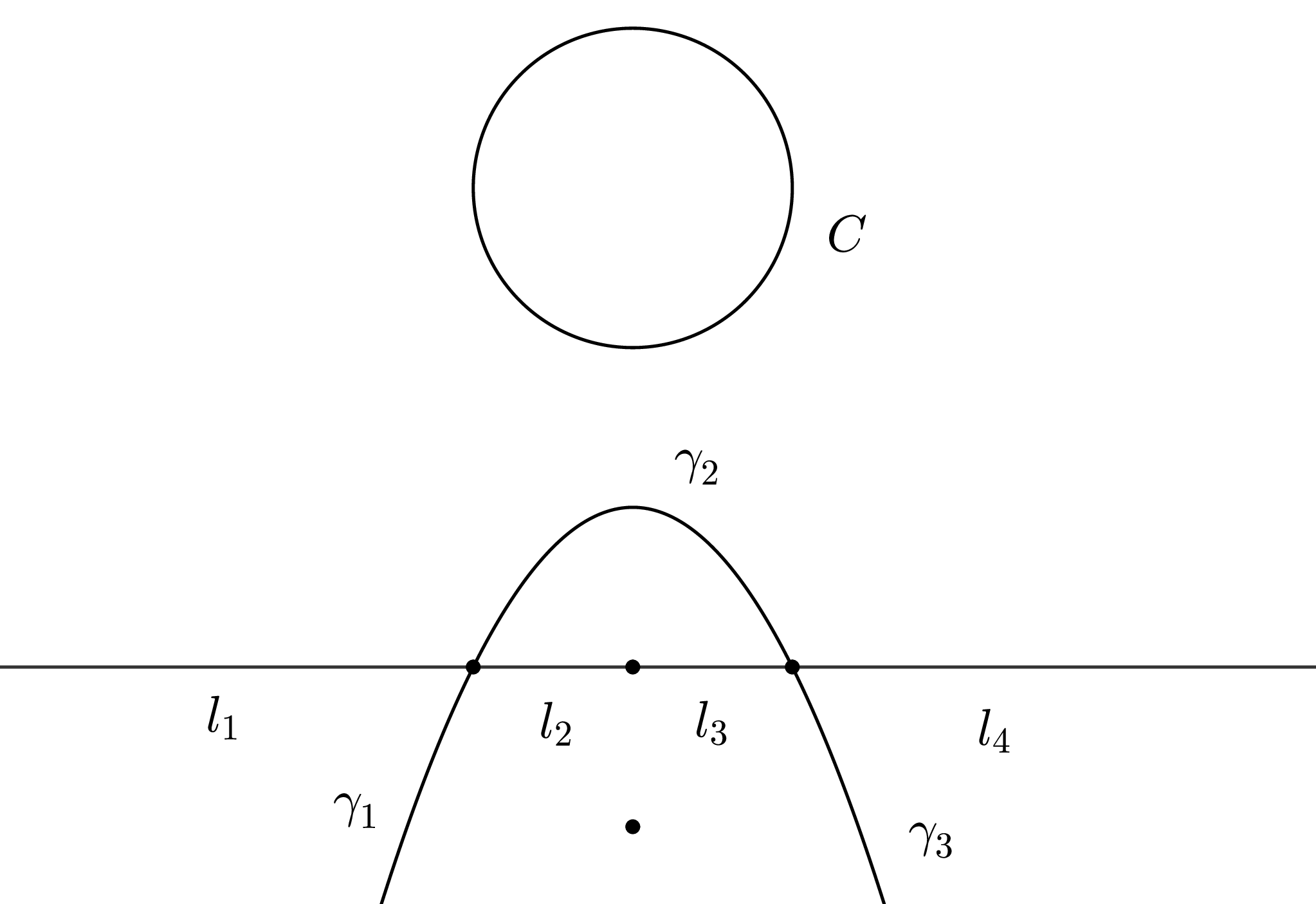
Note since P≥0P\geq 0, then for each fixed xx, the function Q(x,.):ℝ⟶ℝQ(x,.):\mathbb{R}\longrightarrow\mathbb{R} is a homeomorphism. Thus Z:ℝ2⟶ℂZ:\mathbb{R}^{2}\longrightarrow\mathbb{C} is a homeomorphism. The characteristic set of the hypocomplex structure defined by ZZ is given by Σ=P−1​(0)\Sigma=P^{-1}(0). The decomposition of Σ\Sigma is as follows:

  • •

    Σ0={(0,−1)}\ \Sigma^{0}=\{(0,-1)\};

  • •

    S={(−1,0),(0,0),(1,0)}\ S=\{(-1,0),(0,0),(1,0)\}

  • •

    ΣR1=l1∪l2∪l3∪l4∪γ1∪γ2∪γ3∪C\ \Sigma^{1}_{R}=l_{1}\cup l_{2}\cup l_{3}\cup l_{4}\cup\gamma^{1}\cup\gamma_{2}\cup\gamma_{3}\cup C, where l1,⋯,l4l_{1},\cdots,l_{4} are the connected components of the (ℝ×{0})\S(\mathbb{R}\times\{0\})\backslash S, γ1,⋯,γ3\gamma_{1},\cdots,\gamma_{3} are the arc of the connected components {y=1−x2}\S\{y=1-x^{2}\}\backslash S, and CC is the circle x2+(y−3)2=1x^{2}+(y-3)^{2}=1.

Refer to caption
Figure 1. Characteristic set Σ\Sigma

The structure is of type 3 along each segment l1,l2,l3,l4l_{1},\ l_{2},\ l_{3},\ l_{4}; of type 7 along the arcs of parabola γ1,γ2,γ3\gamma_{1},\ \gamma_{2},\ \gamma_{3}; and of type 5 along the circle CC. At the isolated point (0,−1)(0,-1), it is of type 3. At the singular points, it is of type 9 at (−1,0)(-1,0) and (1,0)(1,0) and of type 5 at (0,0)(0,0).

3. Normal forms of first integrals

In this section we derive normal forms for first integrals in neighborhoods of characteristic points of a hypocomplex structure given by (2.3). Throughout, for ϵ\epsilon, δ\delta, and ρ\rho positive numbers, we will denote by DρD_{\rho} the disc with center 00 and radius ρ\rho and by Rϵ,ρR_{\epsilon,\rho} the rectangle in ℝ2\mathbb{R}^{2} given by

Rϵ,ρ={(s,t)∈ℝ2:−1−ϵ<s<1+ϵ,−δ<t<δ}.R_{\epsilon,\rho}=\{(s,t)\in\mathbb{R}^{2}:\ -1-\epsilon<s<1+\epsilon,\ \ -\delta<t<\delta\}\,.

The following proposition can be derived from the general theory of hypoanalytic structures (see [4] or [23])

Proposition 3.1.

Let p∈Σp\in\Sigma. Then there exists a CϖC^{\varpi}-diffeomorphism

Φp:Dρ⟶Uρp=Φp​(Dρ)⊂𝒪;Φp​(0)=p\Phi_{p}:\,D_{\rho}\,\longrightarrow\,U^{p}_{\rho}=\Phi_{p}(D_{\rho})\subset\mathcal{O};\quad\Phi_{p}(0)=p

and a function ψ⁡(s,t)∈Cϖ​(Dρ,ℝ)\psi(s,t)\in C^{\varpi}(D_{\rho};\mathbb{R}) satisfying ψ⁡(0)=0\psi(0)=0 and ψ⁡(s,t)≥0\psi(s,t)\geq 0 for all (s,t)∈D0​(ρ)(s,t)\in D_{0}(\rho) such that the function

(3.1) Zp​(s,t)=s+i​ϕ​(s,t)=s+i​∫0tψ⁡(s,τ)​𝑑τZ_{p}(s,t)=s+i\phi(s,t)=s+i\int_{0}^{t}\psi(s,\tau)d\tau

satisfies d​Φp∗​Z∧d​Zp=0d\Phi_{p}^{\ast}Z\wedge dZ_{p}=0 in DρD_{\rho}. That is ZpZ_{p} is a first integral of the vector field (Φp−1)∗​L(\Phi_{p}^{-1})_{\ast}L.

Remark 3.1.

The type of LL at the point pp can be computed through the normal form ZpZ_{p} and it is the order at t=0t=0 the function ϕ⁡(0,t)\phi(0,t). If p∈Σ0p\in\Sigma^{0} (isolated point in Σ\Sigma), then ZpZ_{p} is a diffeomorphism in the deleted disc Dρ\0D_{\rho}\backslash 0. This implies that ψ⁡(s,t)>0\psi(s,t)>0 for (s,t)≠0(s,t)\neq 0 and that ϕ\phi can be written as ϕ⁡(s,t)=t​ϕ1​(s,t)\phi(s,t)=t\phi_{1}(s,t) with ϕ1​(s,t)>0\phi_{1}(s,t)>0 for (s,t)≠0(s,t)\neq 0.

For p∈Sp\in S, it follows from ψ≥0\psi\geq 0 that there exists r≥1r\geq 1 (odd) such that ϕ⁡(s,t)=tr​ϕ1​(s,t)\phi(s,t)=t^{r}\phi_{1}(s,t) with ϕ1>0\phi_{1}>0 in Dρ\0D_{\rho}\backslash 0. By the Weierstrass Preparation Theorem, we can write ϕ1\phi_{1} in a neighborhood of 0, as

ϕ1​(s,t)=M⁡(s,t)​(t2​l+∑j=12​lAj​(s)​t2​l−j)\phi_{1}(s,t)=M(s,t)\left(t^{2l}+\sum_{j=1}^{2l}A_{j}(s)t^{2l-j}\right)

where MM and the AjA_{j}’s are germs of analytic functions, such that MM is a unit (M⁡(0)≠0M(0)\neq 0), Aj​(0)=0A_{j}(0)=0 for all j=1,⋯2lj=1,\cdots 2l and the order of A2​lA_{2l} is even. The type of LL at pp is k=r+2​lk=r+2l.

Now we construct a normal form along characteristic curves of ΣR1\Sigma^{1}_{R}.

Proposition 3.2.

Let Γ\Gamma be a connected component of ΣR1\Sigma^{1}_{R} and let Γp,q⊂Γ\Gamma_{p,q}\subset\Gamma be an arc connecting two distinct points p,q∈Γp,q\in\Gamma. Let k−1k-1 be the type of LL along Γ\Gamma.Then there exists a CϖC^{\varpi}-diffeomorphism

Φp,q:Rϵ,δ⟶Uϵ,δp,q=Φp,q​(Rϵ,δ)⊂𝒪;Φp,q​(−1,0)=p,Φp,q​(1,0)=q\Phi_{p,q}:\,R_{\epsilon,\delta}\,\longrightarrow\,U^{p,q}_{\epsilon,\delta}=\Phi_{p,q}(R_{\epsilon,\delta})\subset\mathcal{O};\quad\Phi_{p,q}(-1,0)=p,\ \ \Phi_{p,q}(1,0)=q

such that the function

(3.2) Zp,q​(s,t)=s+i​tkZ_{p,q}(s,t)=s+it^{k}

satisfies d​Φp,q∗​Z∧d​Zp,q=0d\Phi_{p,q}^{\ast}Z\wedge dZ_{p,q}=0 in Rϵ,δR_{\epsilon,\delta}. That is Zp,qZ_{p,q} is a first integral of the vector field (Φp,q−1)∗​L(\Phi_{p,q}^{-1})_{\ast}L.

Proof.

First note that since LL is not a (complex) multiple of a tangent vector at any point on Γ\Gamma (otherwise that point of tangency would be a point of infinite type), and since d​Z≠0dZ\neq 0 everywhere, then the restriction of ZZ to Γ\Gamma is a CϖC^{\varpi}-differomorphism. Hence Γ′=Z⁡(Γ)\Gamma^{\prime}=Z(\Gamma) is a 1-dimensional submanifold in ℂ\mathbb{C}. Note also that Z⁡(Σ)Z(\Sigma) is a subanalytic set in ℂ\mathbb{C}. Let Γp,q′=Z⁡(Γp,q)\Gamma_{p,q}^{\prime}=Z(\Gamma_{p,q}) and let UU be an open neighborhood of Γp,q′\Gamma_{p,q}^{\prime} such that U\Γ′U\backslash\Gamma^{\prime} consists of two simply connected components U+U^{+} and U−U^{-} sharing a common boundary along Γ′\Gamma^{\prime}. Let H+:U+¯⟶H+​(U+¯)⊂ℂH^{+}:\overline{U^{+}}\longrightarrow H^{+}(\overline{U^{+}})\subset\mathbb{C} be a conformal map such that

H+(Γ′∩U+¯)⊂ℝ+i0,H+(Z(p))=−1,andH+(Z(q))=1.H^{+}(\Gamma^{\prime}\cap\overline{U^{+}})\,\subset\,\mathbb{R}+i0,\quad H^{+}(Z(p))=-1,\ \ \textrm{and}\ \ H^{+}(Z(q))=1\,.

Since Γ′\Gamma^{\prime} is real analytic, it follows from the Schwarz reflection principle that H+H^{+} can be extended across Γ′\Gamma^{\prime} and into U−U^{-} as a holomorphic HH function defined in a full neighborhood VV of Γp,q′\Gamma_{p,q}^{\prime} and H′​(z)≠0H^{\prime}(z)\neq 0 for every z∈Vz\in V.

Let γ:ℝ⟶Γ\gamma:\mathbb{R}\,\longrightarrow\,\Gamma a CϖC^{\varpi}-parametrization such that γ⁡(−1)=p\gamma(-1)=p, γ⁡(1)=q\ \gamma(1)=q and γ⁡([−1, 1])=Γp,q\gamma([-1,\ 1])=\Gamma_{p,q}. Let η:[−1−ϵ, 1+ϵ]⟶ℝ2\eta:[-1-\epsilon,\ 1+\epsilon]\,\longrightarrow\,\mathbb{R}^{2} be CϖC^{\varpi} and such that η⁡(σ)\eta(\sigma) is a unit normal vector to Γ\Gamma at the point γ⁡(σ)\gamma(\sigma). Define Φp,q\Phi_{p,q} on Rϵ,δR_{\epsilon,\delta} as

Φp,q​(σ,τ)=γ⁡(σ)+τ​η​(σ).\Phi_{p,q}(\sigma,\tau)=\gamma(\sigma)+\tau\eta(\sigma)\,.

Then for ϵ,δ\epsilon,\ \delta small enough Φp,q\Phi_{p,q} is a diffeomorphism onto Uϵ,δp,q=Φp,q​(Rϵ,δ)U^{p,q}_{\epsilon,\delta}=\Phi_{p,q}(R_{\epsilon,\delta}) and

Φp,q​((−1−ϵ, 1+ϵ)×{0})=Uϵ,δp,q∩Σ⊂Γ.\Phi_{p,q}\left((-1-\epsilon,\ 1+\epsilon)\times\{0\}\right)=U^{p,q}_{\epsilon,\delta}\cap\Sigma\,\subset\,\Gamma\,.

That is, the characteristic set of (Φp,q−1)∗​L(\Phi_{p,q}^{-1})_{\ast}L in Rϵ,δR_{\epsilon,\delta} consists of the σ\sigma-axis and each point has finite type k−1k-1. The function

Zp,q​(σ,τ)=H∘Z∘Φp,q​(σ,τ)Z_{p,q}(\sigma,\tau)=H\circ Z\circ\Phi_{p,q}(\sigma,\tau)

is a first integral of (Φp,q−1)∗​L(\Phi_{p,q}^{-1})_{\ast}L. We have Zp,q​(σ,0)∈ℝZ_{p,q}(\sigma,0)\in\mathbb{R} and ∂Zp,q∂σ​(σ,0)≠0\displaystyle\displaystyle\frac{\partial Z_{p,q}}{\partial\sigma}(\sigma,0)\neq 0 for every σ∈(−1−ϵ, 1+ϵ)\sigma\in(-1-\epsilon,\ \ 1+\epsilon). We can therefore (after shrinking ϵ\epsilon and δ\delta if necessary), take s=Re​(Zp,q​(σ,τ)CLOSEs=\textrm{Re}(Z_{p,q}(\sigma,\tau) as a new variable. With respect to the variables (s,τ)(s,\tau) the first integral becomes Zp,q​(s,τ)=s+i​β​(s,τ)Z_{p,q}(s,\tau)=s+i\beta(s,\tau). Since the characteristic set τ=0\tau=0 has type k−1k-1, then β\beta has the form β⁡(s,τ)=τk​β1​(s,τ)\beta(s,\tau)=\tau^{k}\beta_{1}(s,\tau) with β1​(s,0)≠0\beta_{1}(s,0)\neq 0 for all ss. Finally the with respect to the coordinates (s,t)(s,t) with t=τ​β1​(s,τ)k\displaystyle t=\tau\,\sqrt[k]{\beta_{1}(s,\tau)}, the first integral Zp,qZ_{p,q} has the desired form (3.2) ∎

By using similar arguments as those used in the previous proposition, we can prove the following.

Proposition 3.3.

Let Γ⊂ΣR1\Gamma\subset\Sigma^{1}_{R} be a closed curve. Assume that LL is of type k−1k-1 along Γ\Gamma. Then there exists a CϖC^{\varpi}-diffeomorphism

ΦΓ:𝕊1×(−δ,δ)⟶UδΓ=ΦΓ​(𝕊1×(−δ,δ))⊂𝒪;ΦΓ​(𝕊1×{0})=Γ\Phi_{\Gamma}:\,\mathbb{S}^{1}\times(-\delta,\ \delta)\,\longrightarrow\,U^{\Gamma}_{\delta}=\Phi_{\Gamma}(\mathbb{S}^{1}\times(-\delta,\ \delta))\subset\mathcal{O};\quad\Phi_{\Gamma}\left(\mathbb{S}^{1}\times\{0\}\right)=\Gamma

such that the function

(3.3) ZΓ=etk+i​θZ_{\Gamma}=\mathrm{e}^{t^{k}+i\theta}\,

where θ\theta is the angular variable on 𝕊1\mathbb{S}^{1}, satisfies d​ΦΓ∗​Z∧d​ZΓ=0d\Phi_{\Gamma}^{\ast}Z\wedge dZ_{\Gamma}=0 in 𝕊1×(−δ,δ)\mathbb{S}^{1}\times(-\delta,\ \delta). That is ZΓZ_{\Gamma} is a first integral of the vector field (ΦΓ−1)∗​L(\Phi_{\Gamma}^{-1})_{\ast}L.

We will refer to (Uρp,Φp,Zp)\left(U^{p}_{\rho},\Phi_{p},Z_{p}\right) , (Uϵ,δp,q,Φp,q,Zp,q)\left(U^{p,q}_{\epsilon,\delta},\Phi_{p,q},Z_{p,q}\right), and (UδΓ,ΦΓ,ZΓ)\left(U^{\Gamma}_{\delta},\Phi_{\Gamma},Z_{\Gamma}\right) given in Propositions 3.1, 3.2, and 3.3, as charts of normal forms for the vector field LL or the first integral ZZ.

4. Łojasiewicz numbers for the vector field LL

The Łojasiewicz inequality (see [7], [13] for example) found its way as an important tool in many areas including Algebraic Geometry, Differential Equations, and Optimization. The version of the inequality that we will use is the following. Given an open set U⊂ℝnU\subset\mathbb{R}^{n}, and ℝ\mathbb{R}-valued real analytic functions ff and gg defined on UU. If f−1​(0)⊂g−1​(0)f^{-1}(0)\subset g^{-1}(0), then for every compact set K⊂⊂UK\subset\subset U, there exist positive constants CC and μ\mu such that

(4.1) |f⁡(x)|≥C​|g⁡(x)|μ∀x∈K.\lvert f(x)\rvert\geq C\lvert g(x)\rvert^{\mu}\qquad\forall x\in K\,.

We are going to associate a positive number to a hypocomplex structure defined by a real analytic vector field LL. This number is defined through the Łojasiewicz exponent appearing in inequality (4.1) and is linked to the type of the vector field. We start with a normal form chart (Uϵ,δp,q,Φp,q,Zp,q)\left(U^{p,q}_{\epsilon,\delta},\Phi_{p,q},Z_{p,q}\right) about the characteristic arc Γp,q\Gamma_{p,q} along which LL is of type kk, with normal first integral Zp,q​(s,t)=s+i​tkZ_{p,q}(s,t)=s+it^{k}. It follows from the inequality |tk−bk|≥|t−b|k\lvert t^{k}-b^{k}\rvert\geq\lvert t-b\rvert^{k} for all t,b∈ℝt,b\in\mathbb{R}, that

(4.2) |Zp,q​(s,t)−Zp,q​(a,b)|2≥(s−a)2+(t−b)2​k∀(s,t),(a,b)∈Rϵ,δ.\lvert Z_{p,q}(s,t)-Z_{p,q}(a,b)\rvert^{2}\,\geq\,{(s-a)^{2}+(t-b)^{2k}}\quad\forall(s,t),\,(a,b)\in R_{\epsilon,\delta}\,.

We refer to kk as the Łojasiewicz number of LL in the chart (Uϵ,δp,q,Φp,q,Zp,q)\left(U^{p,q}_{\epsilon,\delta},\Phi_{p,q},Z_{p,q}\right).

For p∈Σ0∪Sp\in\Sigma^{0}\cup S, let (Uρp,Φp,Zp)\left(U^{p}_{\rho},\Phi_{p},Z_{p}\right) be the normal form chart about the point pp with Zp​(s,t)=s+i​ϕ​(s,t)Z_{p}(s,t)=s+i\phi(s,t) and ϕ⁡(s,t)=tr​ϕ1​(s,t)\phi(s,t)=t^{r}\phi_{1}(s,t) and ϕ1​(s,t)>0\phi_{1}(s,t)>0 for (s,t)≠(0,0)(s,t)\neq(0,0) such that r=1r=1 when p∈Σ0p\in\Sigma_{0}, and r≥1r\geq 1 (odd number) when p∈Sp\in S (see Remark 3.1). We can assume without loss of generality that ϕ\phi is defined in an open set containing the closed disc Dρ¯\overline{D_{\rho}}. Consider the real analytic functions FF and GG given in ℝ4\mathbb{R}^{4} by

{F⁡((s,t),(a,b))=(s−a)22+[ϕ⁡(s,t)−ϕ⁡(a,b)]2G⁡((s,t),(a,b))=(t−b)2\left\{\begin{array}[]{ll}F\left((s,t),(a,b)\right)&=\displaystyle\frac{(s-a)^{2}}{2}+\left[\phi(s,t)-\phi(a,b)\right]^{2}\\ \\ G\left((s,t),(a,b)\right)&=\displaystyle(t-b)^{2}\end{array}\right.

We have G−1(0)={t=b}G^{-1}(0)=\{t=b\} and since the function ZpZ_{p} is a homeomorphism, then F−1​(0)={s=a,t=b}F^{-1}(0)=\{s=a,\ t=b\}. Clearly F−1​(0)⊂G−1​(0)F^{-1}(0)\subset G^{-1}(0). Therefore, it follows from (4.1) that there exist C=C⁡(ρ)>0C=C(\rho)>0 and μ=μ⁡(ρ)>0\mu=\mu(\rho)>0 such that

(4.3) (s−a)22+[ϕ⁡(s,t)−ϕ⁡(a,b)]2≥C​|t−b|2​μ∀(s,t),(a,b)∈Dρ​(0)¯.\displaystyle\frac{(s-a)^{2}}{2}+\left[\phi(s,t)-\phi(a,b)\right]^{2}\geq C\lvert t-b\rvert^{2\mu}\quad\forall(s,t),\ (a,b)\in\overline{D_{\rho}(0)}.

Define the Łojasiewicz exponent at the point pp as

(4.4) μp=inf{μ>0;∃C>0,ρ>0,(4.3) holds inDρ2}\mu_{p}=\inf\left\{\mu>0;\ \exists C>0,\,\rho>0,\ \text{(\ref{LojIneq11})\ {holds in}}\ D_{\rho}^{2}\right\}
Lemma 4.1.

Let kk and μp\mu_{p} be the type and the Łojasiewicz exponent of LL at the point p∈Σp\in\Sigma. Then k=μpk=\mu_{p}.

Proof.

First recall (Remark 3.1) that the type kk of LL at the point pp is the order at t=0t=0 of the function ϕ⁡(0,t)\phi(0,t). Suppose p∈Σ0∪Sp\in\Sigma^{0}\cup S. By taking s=a=0s=a=0 and b=0b=0 in inequality (4.3) we get |ϕ⁡(0,t)|≥C​|t|μ\lvert\phi(0,t)\rvert\geq C\lvert t\rvert^{\mu} for |t|<ρ\lvert t\rvert<\rho. Therefore μ≥k\mu\geq k and so μp≥k\mu_{p}\geq k. To prove equality, suppose, by contradiction that μp>k\mu_{p}>k. Let μ0\mu_{0} such that k<μ0<μpk<\mu_{0}<\mu_{p}. It follows from the definition of μp\mu_{p} that there exist sequence of points {An=(an,bn)}n∈ℤ+\{A_{n}=(a_{n},b_{n})\}_{n\in\mathbb{Z}^{+}} and {Xn=(sn,tn)}n∈ℤ+\{X_{n}=(s_{n},t_{n})\}_{n\in\mathbb{Z}^{+}} with An,Xn,∈D1/nA_{n},\ X_{n},\in D_{1/n} and

(4.5) (sn−an)22+[ϕ⁡(Xn)−ϕ⁡(An)]2<|tn−bn|2​μ0∀n∈ℤ+\frac{(s_{n}-a_{n})^{2}}{2}+\left[\phi(X_{n})-\phi(A_{n})\right]^{2}\,<\,\lvert t_{n}-b_{n}\rvert^{2\mu_{0}}\quad\forall n\in\mathbb{Z}^{+}

Set sn−an=αns_{n}-a_{n}=\alpha_{n} and tn−bn=βnt_{n}-b_{n}=\beta_{n} and expand the function ϕ\phi into its Taylor series about the point AnA_{n} as

ϕ⁡(Xn)−ϕ⁡(An)=∑i+j≥1,i≥1∂i+jϕ⁡(An)∂si​∂tj​αni​βnji!​j!+∑j=0∞∂jϕ⁡(An)∂tj​βnjj!.\phi(X_{n})-\phi(A_{n})=\sum_{i+j\geq 1,\ i\geq 1}\frac{\partial^{i+j}\phi(A_{n})}{\partial s^{i}\partial t^{j}}\frac{\alpha_{n}^{i}\beta_{n}^{j}}{i!\,j!}+\sum_{j=0}^{\infty}\frac{\partial^{j}\phi(A_{n})}{\partial t^{j}}\frac{\beta_{n}^{j}}{j!}\,.

Note that it follows from (4.5) and k<μ0k<\mu_{0} that limn→∞αnβnk=0\displaystyle\lim_{n\to\infty}\frac{\alpha_{n}}{\beta_{n}^{k}}=0. It also follows from the uniform convergence of Taylor series that

(4.6) limn→∞∑i+j≥1,i≥1∂i+jϕ⁡(An)∂si​∂tj​αni​βnjβnk​i!​j!=0.\lim_{n\to\infty}\sum_{i+j\geq 1,\ i\geq 1}\frac{\partial^{i+j}\phi(A_{n})}{\partial s^{i}\partial t^{j}}\frac{\alpha_{n}^{i}\beta_{n}^{j}}{\beta_{n}^{k}i!\,j!}=0.

To see why (4.6) holds, we can use the Cauchy integral formula to the complexified function ϕ^​(s^,t^)\hat{\phi}(\hat{s},\hat{t}) in a closed bidisc D⁡(ρ)¯2⊂ℂ2\overline{D(\rho)}^{2}\subset\mathbb{C}^{2} with ρ>0\rho>0 small to get estimates of the derivatives

|∂i+jϕ^​(s^,t^)∂s^i​∂t^j|≤4​π2​M​i!​j!(ρ/2)i​(ρ/2)j∀(s^,t^)∈D​(ρ/2)2,\left|\frac{\partial^{i+j}\hat{\phi}(\hat{s},\hat{t})}{\partial\hat{s}^{i}\partial\hat{t}^{j}}\right|\leq 4\pi^{2}M\frac{i!\,j!}{(\rho/2)^{i}(\rho/2)^{j}}\quad\forall(\hat{s},\hat{t})\in D(\rho/2)^{2}\,,

where M=max|s^|=|t^|=ρ⁡|ϕ^​(s^,t^)|\displaystyle M=\max_{|\hat{s}|=|\hat{t}|=\rho}\lvert\hat{\phi}(\hat{s},\hat{t})\rvert. In particular, for nn large enough, we have

|∂i+jϕ⁡(An)∂si​∂tj|≤4​π2​M​i!​j!(ρ/2)i​(ρ/2)j.\left|\frac{\partial^{i+j}\phi(A_{n})}{\partial s^{i}\partial t^{j}}\right|\leq 4\pi^{2}M\frac{i!\,j!}{(\rho/2)^{i}(\rho/2)^{j}}\,.

Consequently, for nn large enough so that αn<ρ/2\alpha_{n}<\rho/2 and βn<ρ/2\beta_{n}<\rho/2, we have

|∑i+j≥1,i≥1∂i+jϕ⁡(An)∂si​∂tj​αni​βnjβnk​i!​j!|≤4​π2​M​ρ2(ρ−2​αn)​(ρ−2​βn)​2​αnβnk\left|\sum_{i+j\geq 1,\ i\geq 1}\frac{\partial^{i+j}\phi(A_{n})}{\partial s^{i}\partial t^{j}}\frac{\alpha_{n}^{i}\beta_{n}^{j}}{\beta_{n}^{k}i!\,j!}\right|\leq\frac{4\pi^{2}M\rho^{2}}{(\rho-2\alpha_{n})(\rho-2\beta_{n})}\,\frac{2\alpha_{n}}{\beta_{n}^{k}}

and the limit in (4.6) follows. As a consequence, we obtain after dividing (4.5) by βn2​k\beta_{n}^{2k} and taking the limit that

limn→∞(∑j=0∞∂jϕ⁡(An)∂tj​βnjj!​βnk)=0.\lim_{n\to\infty}\left(\sum_{j=0}^{\infty}\frac{\partial^{j}\phi(A_{n})}{\partial t^{j}}\frac{\beta_{n}^{j}}{j!\,\beta_{n}^{k}}\right)=0.

This is a contradiction since ∂jϕ⁡(0)∂tj=0\displaystyle\frac{\partial^{j}\phi(0)}{\partial t^{j}}=0 for j<kj<k and ∂kϕ⁡(0)∂tk≠0\displaystyle\frac{\partial^{k}\phi(0)}{\partial t^{k}}\neq 0. ∎

Consequently

(4.7) |Zp​(s,t)−Zp​(a,b)|2≥M⁡((s−a)2+|t−b|2​μ0)∀(s,t),(a,b)∈Dρ¯,\lvert Z_{p}(s,t)-Z_{p}(a,b)\rvert^{2}\,\geq\,M\left({(s-a)^{2}+\lvert t-b\rvert^{2\mu_{0}}}\right)\quad\forall(s,t),\,(a,b)\in\overline{D_{\rho}}\,,

with M=min⁡(12,C)M=\displaystyle\min\left(\frac{1}{2},C\right). We refer to μ0=k\mu_{0}=k as the Łojasiewicz number of LL in the chart (Uρp,Φp,Zp)\left(U^{p}_{\rho},\Phi_{p},Z_{p}\right).

Let Ω\Omega be open, relatively compact, and Ω⊂⊂𝒪\Omega\subset\subset\mathcal{O}. Then ΣΩ=Σ∩Ω¯\Sigma_{\Omega}=\Sigma\cap\overline{\Omega} can be covered by a finite number of open sets U1,⋯,UNU_{1},\cdots,U_{N} such that each UjU_{j} is a normal form chart for the vector field LL. Let μj\mu_{j} be the Łojasiewicz number of LL in UjU_{j}. We define the Łojasiewicz number of LL in Ω\Omega as

(4.8) μ=μ⁡(L,Ω)=max⁡{μ1,⋯,μN}.\mu=\mu(L,\Omega)=\max\{\mu_{1},\cdots,\mu_{N}\}\,.
Remark 4.1.

The definition (4.8) simply means that the Łojasiewicz number of LL in Ω¯\overline{\Omega} is obtained by taking the largest type of LL in Ω¯\overline{\Omega}, which is a finite number because the vector field is real analytic and Ω\Omega is bounded. This number is also invariant under change of coordinates and does not depend on the open sets U1,⋯,UNU_{1},\cdots,U_{N}.

5. Estimate for a generalized Cauchy kernel

We establish an integral estimate that will be crucial in the solvability of the vector field LL. We start with a simple lemma.

Lemma 5.1.

Let 0<τ<10<\tau<1 and 1<q<1+τ1<q<1+\tau. There exists a positive constant C=C⁡(τ,q)C=C(\tau,q) such that for ρ>0\rho>0 we have

(5.1) I=∫Dρd​s​d​t|s+i​|t|1/τ|q≤C​max⁡(ρ1+τ−q,ρ(1+τ−q)/τ)I=\int_{D_{\rho}}\frac{ds\,dt}{\lvert s+i|t|^{1/\tau}\rvert^{q}}\leq C\max(\rho^{1+\tau-q},\rho^{(1+\tau-q)/\tau})
Proof.

For t≠0t\neq 0 consider the new variable η=t|t|​|t|1/τ\eta=\displaystyle\frac{t}{|t|}\lvert t\rvert^{1/\tau} so that d​t=τ​|η|τ−1dt=\tau\lvert\eta\rvert^{\tau-1} and for ρ′=max⁡(ρ,ρ1/τ)\rho^{\prime}=\max(\rho,\rho^{1/\tau}) the integral can be estimated with the use of polar coordinates as

I≤∫Dρ′τ​d​s​d​η|η|1−η​|s+i​η|q=(∫02​πτ​d​θ|sin⁡θ|1−τ)​∫0ρ′rτ−q​𝑑rI\leq\int_{D_{\rho^{\prime}}}\frac{\tau ds\,d\eta}{\lvert\eta\rvert^{1-\eta}\,\lvert s+i\eta\rvert^{q}}=\left(\int_{0}^{2\pi}\frac{\tau d\theta}{\lvert\sin\theta\rvert^{1-\tau}}\right)\int_{0}^{\rho^{\prime}}r^{\tau-q}dr

and (5.1) follows. ∎

Let 𝒪⊂ℝ2\mathcal{O}\subset\mathbb{R}^{2} be open and connected and Z:𝒪⟶Z⁡(𝒪)⊂ℂZ:\mathcal{O}\,\longrightarrow\,Z(\mathcal{O})\subset\mathbb{C} be a real analytic homeomorphism and let L=Zy∂x−Zx∂yL=\displaystyle Z_{y}\partial_{x}-Z_{x}\partial_{y}. For (x,y)(x,y) and (ξ,η)(\xi,\eta) distinct points in 𝒪\mathcal{O}, consider the function 𝒦(x,y)​(ξ,η)\mathcal{K}_{(x,y)}(\xi,\eta) given by

(5.2) 𝒦(x,y)​(ξ,η)=1Z⁡(ξ,η)−Z⁡(x,y).\mathcal{K}_{(x,y)}(\xi,\eta)=\frac{1}{Z(\xi,\eta)-Z(x,y)}\,.

We have the following proposition

Proposition 5.1.

Let Ω⊂𝒪\Omega\subset\mathcal{O} be open and relatively compact and let μ=μ⁡(L,Ω)\mu=\mu(L,\Omega) be the Łojasiewicz number of LL on Ω\Omega. Then for 1<q<1+1μ\displaystyle 1<q<1+\frac{1}{\mu}, we have 𝒦(x,y)∈Lq​(Ω)\mathcal{K}_{(x,y)}\in L^{q}(\Omega). Moreover, there exists a positive constant C=C⁡(Ω,q,μ)C=C(\Omega,q,\mu) such that

(5.3) ‖𝒦(x,y)‖Lq​(Ω)≤C∀(x,y)∈𝒪.\left\lVert\mathcal{K}_{(x,y)}\right\rVert_{L^{q}(\Omega)}\leq C\qquad\forall(x,y)\in\mathcal{O}\,.

The remainder of this section deals with the proof of the proposition. We start by proving (5.3) in the case of a normal form

Lemma 5.2.

Let Z0​(s,t)=s+i​ϕ​(s,t)Z_{0}(s,t)=s+i\phi(s,t) with ϕ∈Cϖ​(Dρ,ℝ)\phi\in C^{\varpi}(D_{\rho};\mathbb{R}), ϕ⁡(s,t)=tr​ϕ1​(s,t)\,\phi(s,t)=t^{r}\phi_{1}(s,t) with r∈ℤ+r\in\mathbb{Z}^{+} and ϕ1​(s,t)>0\phi_{1}(s,t)>0 for (s,t)≠0(s,t)\neq 0, and such that Z0:Dρ⟶Z0​(Dρ)Z_{0}:D_{\rho}\longrightarrow Z_{0}(D_{\rho}) is a homeomorphism. Let μ0\mu_{0} be the associated Łojasiewicz number of the induced hypocomplex structure and let 1<q<1+1μ0\displaystyle 1<q<1+\frac{1}{\mu_{0}}. Then there exists C=C⁡(ρ,μ0,q)C=C(\rho,\mu_{0},q) such that

(5.4) Iw=∫Dρ/2d​s​d​t|Z0​(s,t)−w|q≤C∀w∈ℂ.I_{w}=\int_{D_{\rho/2}}\frac{ds\,dt}{\lvert Z_{0}(s,t)-w\rvert^{q}}\,\leq\,C\qquad\forall w\in\mathbb{C}\,.
Proof.

If w∉Z0​(Dρ)w\notin Z_{0}(D_{\rho}), then there exists δ>0\delta>0 such that

|Z0​(s,t)−w|≥δ∀(s,t)∈Dρ/2.\lvert Z_{0}(s,t)-w\rvert\geq\delta\qquad\forall(s,t)\in D_{\rho/2}\,.

Therefore

Iw≤π​ρ24​δq.I_{w}\leq\frac{\pi\rho^{2}}{4\delta^{q}}\,.

For w∈Z0​(Dρ)w\in Z_{0}(D_{\rho}), let (a,b)∈Dρ(a,b)\in D_{\rho} such that w=Z0​(a,b)w=Z_{0}(a,b). In this case the Łojasiewicz inequality implies that

|Z0​(s,t)−w|2=|Z0​(s,t)−Z0​(a,b)|2≥Cρ​[(s−a)2+(t−b)2​μ0]\lvert Z_{0}(s,t)-w\rvert^{2}=\lvert Z_{0}(s,t)-Z_{0}(a,b)\rvert^{2}\geq C_{\rho}\left[(s-a)^{2}+(t-b)^{2\mu_{0}}\right]

and, after using Dρ/2⊂D⁡((a,b),2​ρ)D_{\rho/2}\subset D((a,b),2\rho) and applying Lemma (5.1), we get

Iw≤1Cρ​∫Dρ/2d​s​d​t[(s−a)2+(t−b)2​μ0]q/2≤1Cρ​∫D⁡((a,b),2​ρ)d​s​d​t[(s−a)2+(t−b)2​μ0]q/2≤1Cρ​∫D2​ρd​s​d​t|s+i​|t|μ0|q≤C⁡(ρ,μ0,q)\begin{array}[]{ll}I_{w}&\displaystyle\leq\frac{1}{C_{\rho}}\int_{D_{\rho/2}}\frac{ds\,dt}{\left[(s-a)^{2}+(t-b)^{2\mu_{0}}\right]^{q/2}}\\ \\ &\displaystyle\leq\frac{1}{C_{\rho}}\int_{D((a,b),2\rho)}\frac{ds\,dt}{\left[(s-a)^{2}+(t-b)^{2\mu_{0}}\right]^{q/2}}\\ \\ &\displaystyle\leq\frac{1}{C_{\rho}}\int_{D_{2\rho}}\frac{ds\,dt}{\lvert s+i|t|^{\mu_{0}}\rvert^{q}}\leq C(\rho,\mu_{0},q)\end{array}

∎

Similar arguments show that in a normal form chart (Uϵ,δp,q,Φp,q,Zp,q)\left(U^{p,q}_{\epsilon,\delta},\Phi_{p,q},Z_{p,q}\right) about the characteristic arc Γp,q\Gamma_{p,q} along which LL is of type k−1k-1, with normal first integral Zp,q​(s,t)=s+i​tkZ_{p,q}(s,t)=s+it^{k}, we have

(5.5) Iw=∫Rϵ/2,δ/2d​s​d​t|Zp,q​(s,t)−w|q≤C∀w∈ℂ.I_{w}=\int_{R_{\epsilon/2,\delta/2}}\frac{ds\,dt}{\lvert Z_{p,q}(s,t)-w\rvert^{q}}\,\leq\,C\qquad\forall w\in\mathbb{C}\,.

Now we continue with the proof of the proposition. Let ΣΩ=Σ∩Ω¯\Sigma_{\Omega}=\Sigma\cap\overline{\Omega}. Then ΣΩ\Sigma_{\Omega} can be covered by a finite number of normal form charts U1,⋯,UNU_{1},\,\cdots\,,U_{N}. Hence for j=1,⋯,Nj=1,\cdots,N, there exists a diffeomorphism Φj:Vj⟶Uj\Phi_{j}:V_{j}\,\longrightarrow\,U_{j} with Vj=DρV_{j}=D_{\rho} or Vj=Rϵ,δV_{j}=R_{\epsilon,\delta}. Denote by ZjZ_{j} the normal form of the first integral in VjV_{j}. Let Vj′=Dρ/2V_{j}^{\prime}=D_{\rho/2} or Vj′=Rϵ/2,δ/2V_{j}^{\prime}=R_{\epsilon/2,\delta/2}, respectively, and let Uj′=Φj​(Vj′)U^{\prime}_{j}=\Phi_{j}(V^{\prime}_{j}). We can assume that ΣΩ⊂⋃j=1NUj′\displaystyle\Sigma_{\Omega}\subset\bigcup_{j=1}^{N}U^{\prime}_{j}. After shrinking ρ\rho, ϵ\epsilon and δ\delta, if necessary, we can find conformal maps HjH_{j} defined on open neighborhoods of Zj​(Vj)¯\overline{Z_{j}(V_{j})} such that

(5.6) Z⁡(x,y)=Hj​(Zj​(Φj−1​(x,y)))in​Uj,j=1,⋯,N.Z(x,y)=H_{j}\left(Z_{j}\left(\Phi_{j}^{-1}(x,y)\right)\right)\ \ \text{in}\ U_{j},\qquad j=1,\cdots,N\,.

For j=1,⋯,Nj=1,\cdots,N, consider the positive constants

cj=infz∈Zj​(Vj)|Hj′​(z)|andMj=sup(s,t)∈Vj|D​Φj​(s,t)|c_{j}=\inf_{z\in Z_{j}(V_{j})}\lvert H_{j}^{\prime}(z)\rvert\quad\text{and}\quad M_{j}=\sup_{(s,t)\in V_{j}}\lvert D\Phi_{j}(s,t)\rvert

and, for (x,y)∈𝒪(x,y)\in\mathcal{O}, the integral

(5.7) Ij=∫Uj′|𝒦(x,y)​(ξ,η)|q​𝑑ξ​𝑑ηI_{j}=\int_{U^{\prime}_{j}}\lvert\mathcal{K}_{(x,y)}(\xi,\eta)\rvert^{q}d\xi\,d\eta

If (x,y)∉Uj(x,y)\notin U_{j}, then there exists δj>0\delta_{j}>0 such that |𝒦(x,y)​(ξ,η)|≥δ\lvert\mathcal{K}_{(x,y)}(\xi,\eta)\rvert\geq\delta, ∀(ξ,η)∈Uj′\forall(\xi,\eta)\in U^{\prime}_{j} and in this case

(5.8) Ij≤Area​(Uj′)δjq∀(x,y)∈𝒪\Uj.I_{j}\leq\frac{\text{Area}(U^{\prime}_{j})}{\delta_{j}^{q}}\qquad\forall(x,y)\in\mathcal{O}\backslash U_{j}\,.

If (x,y)∈Uj(x,y)\in U_{j}, then there exist (a,b)∈Vj(a,b)\in V_{j} such that (x,y)=Φj​(a,b)(x,y)=\Phi_{j}(a,b). Also (ξ,η)∈Uj(\xi,\eta)\in U_{j} can be written as (ξ,η)=Φj​(s,t)(\xi,\eta)=\Phi_{j}(s,t) with (s,t)∈Vj(s,t)\in V_{j}. Hence,

|𝒦(x,y)​(ξ,η)|=1|Hj​(Zj​(s,t))−Hj​(Zj​(a,b))|≤1cj​|Zj​(s,t)−Zj​(a,b)|.\lvert\mathcal{K}_{(x,y)}(\xi,\eta)\rvert=\frac{1}{\lvert H_{j}\left(Z_{j}(s,t)\right)-H_{j}\left(Z_{j}(a,b)\right)\rvert}\leq\,\frac{1}{c_{j}\,\lvert Z_{j}(s,t)-Z_{j}(a,b)\rvert}\,.

It follows from this inequality, (5.4) and (5.5)that

(5.9) Ij≤1cjq​∫Vj′|D⁡(Φj​(s,t))|​d​s​d​t|Zj​(s,t)−Zj​(a,b)|q≤Mjcjq​∫Vj′d​s​d​t|Zj​(s,t)−Zj​(a,b)|q≤Cj∀(x,y)∈Uj\begin{array}[]{ll}I_{j}&\displaystyle\leq\frac{1}{c_{j}^{q}}\int_{V_{j}^{\prime}}\frac{\lvert D(\Phi_{j}(s,t))\rvert\,ds\,dt}{\lvert Z_{j}(s,t)-Z_{j}(a,b)\rvert^{q}}\\ \\ &\displaystyle\leq\frac{M_{j}}{c_{j}^{q}}\int_{V_{j}^{\prime}}\frac{ds\,dt}{\lvert Z_{j}(s,t)-Z_{j}(a,b)\rvert^{q}}\leq C_{j}\qquad\forall(x,y)\in U_{j}\end{array}

for some constant CjC_{j} depending on UjU_{j}, qq, and the Łojasiewicz number μj\mu_{j} in UjU_{j}. It follows then from (5.8) and (5.9) that for every j=1,⋯Nj=1,\cdots N there exists Bj=Bj​(Uj,q,μj)B_{j}=B_{j}(U_{j},q,\mu_{j}) such that

(5.10) Ij≤Bj∀(x,y)∈𝒪.I_{j}\leq B_{j}\qquad\forall(x,y)\in\mathcal{O}\,.

Let Ω0=Ω\(⋃j=1NUj′)\displaystyle\Omega_{0}=\Omega\backslash\left(\bigcup_{j=1}^{N}U_{j}^{\prime}\right). The structure induced by ZZ is elliptic in an open neighborhood of Ω0\Omega_{0} and therefore 𝒦(x,y)​(ξ,η)\mathcal{K}_{(x,y)}(\xi,\eta) is conjugate to the classical Cauchy kernel 1ζ−z\displaystyle\frac{1}{\zeta-z} and it follows that there exists a positive constant B0=B0​(Ω0,q)B_{0}=B_{0}(\Omega_{0},q) such that

(5.11) I0=∫Ω0|𝒦(x,y)​(ξ,η)|q​𝑑ξ​𝑑η≤B0∀(x,y)∈𝒪.I_{0}=\int_{\Omega_{0}}\lvert\mathcal{K}_{(x,y)}(\xi,\eta)\rvert^{q}\,d\xi\,d\eta\,\leq\,B_{0}\qquad\forall(x,y)\in\mathcal{O}.

Finally, for 1<q<1+1μ≤1+1μj\displaystyle 1<q<1+\frac{1}{\mu}\leq 1+\frac{1}{\mu_{j}}, j=1,⋯,Nj=1,\cdots,N we have

‖𝒦(x,y)‖Lq​(Ω)≤∑j=0NIj≤∑j=0NBj∀(x,y)∈𝒪.\left\lVert\mathcal{K}_{(x,y)}\right\rVert_{L^{q}(\Omega)}\leq\sum_{j=0}^{N}I_{j}\,\leq\,\sum_{j=0}^{N}B_{j}\qquad\forall(x,y)\in\mathcal{O}\ .

6. Generalized Cauchy Operator

A generalization of the Cauchy integral operator for vector fields in two variables appeared in papers [16], [17], [18] and then in [10] and [11]. Here we use the generalized Cauchy operator for real analytic hypocomplex structures given by a vector filed (2.3) with a global first integral ZZ on the open set 𝒪⊂ℝ2\mathcal{O}\subset\mathbb{R}^{2}. For Ω⊂𝒪\Omega\subset\mathcal{O} open and relatively compact, we consider the operator

(6.1) TZ​u​(x,y)=−1π​∫Ωu⁡(ξ,η)​𝒦(x,y)​(ξ,η)​𝑑ξ​𝑑η=−1π​∫Ωu⁡(ξ,η)Z⁡(ξ,η)−Z⁡(x,y)​𝑑ξ​𝑑η\begin{array}[]{ll}T_{Z}u(x,y)&\displaystyle=\frac{-1}{\pi}\int_{\Omega}u(\xi,\eta)\,\mathcal{K}_{(x,y)}(\xi,\eta)\,d\xi d\eta\\ \\ &\displaystyle=\frac{-1}{\pi}\int_{\Omega}\frac{u(\xi,\eta)}{Z(\xi,\eta)-Z(x,y)}\,d\xi d\eta\end{array}

We have the following theorem

Theorem 6.1.

Let μ=μ⁡(Ω,L)\mu=\mu(\Omega,L) be the Łojasiewicz number of LL on Ω\Omega and let p>1+μp>1+\mu. Then there exists a positive constant M=M⁡(Ω,p,μ)M=M(\Omega,p,\mu) such that

(6.2) |TZ​f​(x,y)|≤M​‖f‖Lp​(Ω)∀f∈Lp​(Ω),∀(x,y)∈𝒪.\lvert T_{Z}f(x,y)\rvert\,\leq\,M\,\left\lVert f\right\rVert_{L^{p}(\Omega)}\qquad\forall f\in L^{p}(\Omega),\ \ \forall(x,y)\in\mathcal{O}\,.
Proof.

For p>1+μp>1+\mu, the Hölder conjugate qq satisfies 1<q<1+1μ\displaystyle 1<q<1+\frac{1}{\mu}. The Hölder inequality gives |TZ​f​(x,y)|≤‖𝒦(x,y)‖Lq​(Ω)​‖f‖Lp​(Ω)\displaystyle\lvert T_{Z}f(x,y)\rvert\,\leq\,\left\lVert{\mathcal{K}_{(x,y)}}\right\rVert_{L^{q}(\Omega)}\,\left\lVert f\right\rVert_{L^{p}(\Omega)} and (6.2) follows from Proposition (5.1). ∎

Proposition 6.1.

Let f∈L1​(Ω)f\in L^{1}(\Omega), then TZ​f∈Lq​(Ω)T_{Z}f\in L^{q}(\Omega) for any qq with 1<q<1+1μ\displaystyle 1<q<1+\frac{1}{\mu}.

Proof.

Let 1<q<1+1μ\displaystyle 1<q<1+\frac{1}{\mu} and p>1+μp>1+\mu be the Hölder conjugate of qq. Let gg be an arbitrary function in Lp​(Ω)L^{p}(\Omega). It follows from Theorem 6.1 that g1​(x,y)∈L∞​(𝒪)g_{1}(x,y)\in L^{\infty}(\mathcal{O}) where g1g_{1} is given by

g1​(x,y)=∫Ω|g⁡(ξ,η)|​|𝒦(x,y)​(ξ,η)|​𝑑ξ​𝑑η.g_{1}(x,y)=\int_{\Omega}\lvert g(\xi,\eta)\rvert\,\lvert\mathcal{K}_{(x,y)}(\xi,\eta)\rvert\,d\xi\,d\eta\,.

Therefore f​g1∈L1​(Ω)fg_{1}\in L^{1}(\Omega). Now we use Fubini’s Theorem together with 𝒦(x,y)​(ξ,η)=−𝒦(ξ,η)​(x,y)\mathcal{K}_{(x,y)}(\xi,\eta)=-\mathcal{K}_{(\xi,\eta)}(x,y) to obtain

∫Ω|f⁡(x,y)|​g1​(x,y)​𝑑x​𝑑y=∫Ω|g⁡(ξ,η)|​(∫Ω|f⁡(x,y)|​|𝒦(ξ,η)​(x,y)|​dx​dy)⏟f1​(ξ,η)​𝑑ξ​𝑑η\displaystyle\int_{\Omega}\lvert f(x,y)\rvert g_{1}(x,y)\,dxdy=\int_{\Omega}\lvert g(\xi,\eta)\rvert\underbrace{\left(\int_{\Omega}\lvert f(x,y)\rvert\,\lvert\mathcal{K}_{(\xi,\eta)}(x,y)\rvert dx\,dy\right)}_{f_{1}(\xi,\eta)}d\xi\,d\eta

This means that g​f1∈L1​(Ω)gf_{1}\in L^{1}(\Omega). Since g∈Lp​(Ω)g\in L^{p}(\Omega) is arbitrary, then the reverse of the Hölder inequality implies that f1∈Lq​(Ω)f_{1}\in L^{q}(\Omega). We have |TZ​f|≤f1\lvert T_{Z}f\rvert\,\leq f_{1}, and so TZ​f∈Lq​(Ω)T_{Z}f\in L^{q}(\Omega). ∎

Arguments similar to those used to prove Proposition 12 in [10] can be applied to establish the following

Proposition 6.2.

Let w∈C⁡(Ω¯)∩C1​(Ω)w\in C(\overline{\Omega})\cap C^{1}(\Omega). Then for every (x,y)∈Ω(x,y)\in\Omega, we have

(6.3) 2​π​i​w​(x,y)=∫∂Ωw⁡(ξ,η)​𝒦(x,y)​(ξ,η)​𝑑Z​(ξ,η)+∫ΩL​w​(ξ,η)​𝒦(x,y)​(ξ,η)​𝑑ζ∧𝑑ζ¯,2\pi iw(x,y)=\int_{\partial\Omega}\!\!\!w(\xi,\eta)\,\mathcal{K}_{(x,y)}(\xi,\eta)\,dZ(\xi,\eta)\,+\int_{\Omega}\!\!\!Lw(\xi,\eta)\,\mathcal{K}_{(x,y)}(\xi,\eta)\,d\zeta\wedge d\overline{\zeta},

where ζ=ξ+i​η\zeta=\xi+i\eta.

Theorem 6.2.

If f∈L1​(Ω)f\in L^{1}(\Omega), then L⁡(TZ​f)=fL(T_{Z}f)=f. In particular if f∈Lp​(Ω)f\in L^{p}(\Omega) with p>1+μp>1+\mu, where μ\mu is the Łojasiewicz number of LL in Ω\Omega, then TZ​fT_{Z}f is an L∞L^{\infty}-solution of the equation L​u=fLu=f.

Proof.

We know from Proposition (6.1) that for f∈L1​(Ω)f\in L^{1}(\Omega), TZ​f∈Lq​(Ω)T_{Z}f\in L^{q}(\Omega) for 1<q<1+1μ\displaystyle 1<q<1+\frac{1}{\mu}. Note that the transpose of the operator LL is Lt=−L{}^{t}L=-L. Let ϕ∈C0∞​(Ω)\phi\in C^{\infty}_{0}(\Omega) be a test function. Then by using (6.3) for ϕ\phi and taking into account that ϕ=0\phi=0 on ∂Ω\partial\Omega, we obtain

⟨L⁡(TZ​f),ϕ⟩=−⟨TZ​f,L​ϕ⟩=∫Ω[1π​∫Ωf⁡(ξ,η)​𝒦(x,y)​(ξ,η)​𝑑ξ​𝑑η]​L​ϕ​(x,y)​𝑑x​𝑑y=∫Ωf⁡(ξ,η)​[12​π​i​∫ΩL​ϕ​(x,y)​𝒦(ξ,η)​(x,y)​𝑑z∧𝑑z¯]​𝑑ξ​𝑑η=⟨f,ϕ⟩\begin{array}[]{ll}\left<L(T_{Z}f),\phi\right>&\displaystyle=-\left<T_{Z}f,L\phi\right>\\ \\ &\displaystyle=\int_{\Omega}\left[\frac{1}{\pi}\int_{\Omega}f(\xi,\eta)\mathcal{K}_{(x,y)}(\xi,\eta)d\xi\,d\eta\right]L\phi(x,y)\,dx\,dy\\ \\ &\displaystyle=\int_{\Omega}f(\xi,\eta)\left[\frac{1}{2\pi i}\int_{\Omega}L\phi(x,y)\mathcal{K}_{(\xi,\eta)}(x,y)dz\wedge d\overline{z}\right]\,d\xi\,d\eta\\ \\ &\displaystyle=\left<f,\phi\right>\end{array}

The second part of the statement of the Theorem follows from Theorem 6.1. ∎

Now we establish a similarity principle between the solutions of the equation L​u=A​u+B​u¯Lu=Au+B\overline{u} and holomorphic functions in Z⁡(Ω)Z(\Omega). More precisely, we have the following

Theorem 6.3.

Let A,B∈Lp​(Ω)A,\,B\,\in L^{p}(\Omega) with p>1+μp>1+\mu, where μ\mu is the Łojasiewicz number of LL in Ω\Omega. If u∈L∞​(Ω)u\in L^{\infty}(\Omega) satisfies the equation

(6.4) L​u=A​u+B​u¯,Lu=Au+B\overline{u}\,,

then there exists a holomorphic function HH in Z⁡(Ω)Z(\Omega) and a function s∈L∞​(Ω)s\in L^{\infty}(\Omega) such that

(6.5) u⁡(x,y)=H⁡(Z⁡(x,y))​es⁡(x,y).u(x,y)=H(Z(x,y))\,\mathrm{e}^{s(x,y)}\,.
Proof.

Let u∈L∞​(Ω)u\in L^{\infty}(\Omega) be a solution of (6.4). Since LL is elliptic in 𝒪\Σ\mathcal{O}\backslash\Sigma, then if u=0u=0 on a set with an accumulation in Ω\Omega, then u=0u=0 everywhere in Ω\Σ\Omega\backslash\Sigma. For uu not identically zero, consider the function χ\chi given by χ=u¯u\displaystyle\chi=\frac{\overline{u}}{u} at the points where u≠0u\neq 0 and χ=0\chi=0 when u=0u=0. Then |χ|≤1\lvert\chi\rvert\leq 1 and A+B​χ∈Lp​(Ω)A+B\chi\in L^{p}(\Omega). It follows from Theorem 6.2 that the function s=TZ​(A+B​χ)∈L∞​(Ω)s=T_{Z}(A+B\chi)\in L^{\infty}(\Omega) and satisfies

(6.6) u​L​s=A​u+B​u¯.uLs=Au+B\overline{u}\,.

Consider the function v∈L∞​(Ω)v\in L^{\infty}(\Omega) given by v=u​e−sv=u\mathrm{e}^{-s}. Then it follows from (6.6) that L​v=0Lv=0 in Ω\Omega. Since LL is hypocomplex, then vv factors as v=H∘Zv=H\circ Z for some holomorphic function HH defined in Z⁡(Ω)Z(\Omega) and (6.5) follows. ∎

Remark 6.4.

The results of this paper are stated for real analytic structures but they can be extended for any structure that satisfies the Łojasiewicz inequality in neighborhoods of points of the characteristic set Σ\Sigma. In particular, if Z:𝒪⟶Z⁡(𝒪)⊂ℂZ:\,\mathcal{O}\,\longrightarrow\,Z(\mathcal{O})\subset\mathbb{C} is C1+αC^{1+\alpha}-homeomorphism (0<α<10<\alpha<1) and if ZZ is real analytic in a tubular neighborhood of Σ\Sigma, then a Łojasiewicz number μ\mu can be attached to LL on any relatively compact open set Ω⊂𝒪\Omega\subset\mathcal{O} and Theorems 6.1, 6.2, and 6.3 hold. In fact the real analyticity of ZZ near Σ\Sigma can also be weakened to only assume that ZZ is in Denjoy-Carleman classes, since functions in these classes satisfy the Łojasiewicz inequality (see [8] or [25]).

Hypotheses on ff and A,BA,\,B in equations L​u=fLu=f and L​u=A​u+B​u¯Lu=Au+B\overline{u} can also be weakened to assume that f,A,Bf,\,A,\,B are in Lp0​(Ω)L^{p_{0}}(\Omega) for some p0>2p_{0}>2 and in Lpi​(Ui)L^{p_{i}}(U_{i}) with pi>1+μip_{i}>1+\mu_{i} in each normal form chart UiU_{i} with Łojasiewicz number μi\mu_{i}.

References

  • [1] H. Begehr, Complex analytic methods for partial differential equations, World Scientific Publishing Co., Inc., River Edge, NJ, 1994
  • [2] A. Bergamasco, P. Cordaro, J. Hounie Global properties of a class of vector fields in the plane, J. Diff. Equations 74 (1988), no. 2, 179-199
  • [3] A. Bergamasco, A. Meziani Solvability near the characteristic set for a class of planar vector fields of infinite type, Ann. Inst. Fourier 55 (2005), no. 1, 77-112
  • [4] S. Berhanu, P. Cordaro, J. Hounie, An introduction to involutive structures. New Mathematical Monographs, 6. Cambridge University Press, Cambridge, 2008
  • [5] S. Berhanu, J. Hounie, P. Santiago A similarity principle for complex vector fields and applications. Trans. Amer. Math. Soc. 353(2001), no. 4, 1661–1675.
  • [6] L. Bers, An outline of the theory of pseudoanalytic functions. Bull. Amer. Math. Soc. 62 (1956), 291-331
  • [7] E. Bierstone, P. Milman, Semianalytic and subanalytic sets. Inst. Hautes Études Sci. Publ. Math. No. 67 (1988), 5–42
  • [8] E. Bierstone, P. Milman, Resolution of singularities in Denjoy-Carleman classes. Selecta Math. (N.S.) 10 (2004), no. 1, 1-28
  • [9] C. Campana, P. Dattori, A. Meziani, Riemann-Hilbert problem for a class of hypocomplex vector fields. Complex Var. Elliptic Equ. 61 (2016), no. 12, 1656–1667.
  • [10] C. Campana, P. Dattori, A. Meziani, Properties of solutions of a class of hypocomplex vector fields. Analysis and geometry in several complex variables, 29–50, Contemp. Math., 681, Amer. Math. Soc., Providence, RI, 2017
  • [11] C. Campana, A. Meziani, Boundary value problems for a class of planar complex vector fields. J. Differential Equations 261 (2016), no. 10, 5609–5636.
  • [12] J. Hounie, G. Zugliani, Tube structures of co-rank 1 with forms defined on compact surfaces. J. Geom. Anal. 31 (2021), no. 3, 2540–2567.
  • [13] S. Łojasiewicz, Sur le problème de la division. Studia Math. 18 (1959), 87-136
  • [14] A. Meziani, On the similarity principle for planar vector fields: application to second order PDE. J. Differential Equations 157 (1999), no. 1, 1–19
  • [15] A. Meziani, On planar elliptic structures with infinite type degeneracy. J. Funct. Anal. 179 (2001), no. 2, 333-373
  • [16] A. Meziani, Elliptic planar vector fields with degeneracies. Trans. Amer. Math. Soc. 357 (2005), no. 10, 4225–4248
  • [17] A. Meziani, Global solvability of real analytic complex vector fields in two variables. J. Differential Equations 251 (2011), no. 10, 2896–2931
  • [18] A. Meziani On first and second order planar elliptic equations with degeneracies. Mem. Amer. Math. Soc. 217 (2012), no. 1019
  • [19] A. Meziani, A. Ainouz, K. Boutarene, The Riemann-Hilbert problem for elliptic vector fields with degeneracies. Complex Var. Elliptic Equ. 59 (2014), no. 6, 751–768
  • [20] A. Meziani, G. Zugliani, Class of hypocomplex structures on the two-dimensional torus. Proc. Amer. Math. Soc. 147 (2019), no. 9, 3937–3946
  • [21] G. Springer, Introduction to Riemann surfaces. Addison-Wesley Publishing Company Inc. Reading Mass. 1957
  • [22] R. Simha, The uniformisation theorem for planar Riemann surfaces. Arch. Math. (Basel) 53 (1989), no. 6, 599–603
  • [23] F. Treves, Hypo-analytic structures: Local theory. Princeton Mathematical Series, 40. Princeton University Press, Princeton, NJ, 1992
  • [24] I. Vekua, Generalized Analytic Functions. Pergamon Press, Oxford, 1962
  • [25] A. Volberg. The Łojasiewicz inequality for very smooth functions. Soviet Math. Dokl. 41 (1990), 170–174