End-to-End Signal Classification in Signed Cumulative Distribution Transform Space
Abstract
This paper presents a new end-to-end signal classification method using the signed cumulative distribution transform (SCDT). We adopt a transport-based generative model to define the classification problem. We then make use of mathematical properties of the SCDT to render the problem easier in transform domain, and solve for the class of an unknown sample using a nearest local subspace (NLS) search algorithm in SCDT domain. Experiments show that the proposed method provides high accuracy classification results while being computationally cheap, data efficient, and robust to out-of-distribution samples with respect to the existing end-to-end classification methods. The implementation of the proposed method in Python language is integrated as a part of the software package PyTransKit [1].
Index Terms:
signal classification, time series events, generative model, SCDT, nearest local subspace.I Introduction
Signal (time series) classification is considered a challenging problem in data science. It refers to the automatic prediction of the class label of an unknown time series event using the information extracted from the corresponding signal intensities. Time series data classification tasks can be found in many applications such as human activity recognition (HAR) [2], physiological signal assessment [3][4], communications [5], structural or machine health monitoring systems [6] [7], financial modeling [8], and others. In many applications (e.g., HAR, ECG, etc.) the time series events of interest can be modeled as instances of a certain (often unknown) template or prototype pattern observed under unknown time warps [9]. Here we propose a new end-to-end tool for classification of signals or time series events of this type using the signed cumulative distribution transform (SCDT), a new mathematical signal transform introduced in [10].
Existing signal classification approaches can be categorized into two broad, and at times overlapping, categories: 1) feature engineering-based classifiers and 2) end-to-end learning classifiers, such as convolutional neural networks (CNNs). Feature engineering-based methods [11] [12] [13] usually rely on the extraction of numerical features (e.g., time domain features, frequency domain features, wavelet features) from the raw signal data, and then the application of different multivariate regression-based classification methods including linear discriminant analysis, support vector machines, random forests, and others. Deep learning-based signal classification methods [14] [15] [16], on the other hand, connect the raw input data to the output class label by utilizing a large number of hidden layers. These methods have widely been studied recently as they have shown high accuracy in certain classification tasks.
Feature engineering signal classification approaches primarily differ in the types of features chosen to characterize each signal. The bag-of-features framework [17] extracts interval features using fixed- and variable-length intervals, and trains a classifier on the extracted features. Ensemble-based approaches such as COTE [18], HIVE-COTE [19], time series forest (TSF) [20], and others combine different features and classifiers to achieve high classification accuracy. Most of these methods require crafting especially designed features (feature engineering) as well as some amount of data preprocessing.
Traditional end-to-end signal classification techniques include distance-based methods [21] [22] that work directly on raw time series with some similarity measures such as Euclidean distance or dynamic time warping (DTW) [23]. Particularly, a combination of -nearest neighbor (1NN) with DTW distance is known to be a very effective time series classification approach [24]. However, it is known to have high computational complexity [25]. Approaches based on deep neural networks, especially convolutional neural networks (CNN) [26], have been explored in recent years for end-to-end signal classification. Wang et al. [27], for example, provided three standard deep learning benchmark models for time series classification: deep multilayer perceptrons (MLP), fully convolutional networks (FCN), and residual networks (ResNet). The method known as multi-scale convolutional neural network (MCNN) [28] is another deep learning approach that takes advantage of CNNs for end-to-end classification of univariate time series. Karim et al. [29] proposed the LSTM-FCN, an improvement over FCN by augmenting the FCN module with a Long Short Term Recurrent Neural Network (LSTM RNN) sub-module. Though they can produce accurate results in many instances, these methods tend to require extensive amounts of training data, are computationally expensive, and often vulnerable to out-of-distribution examples. Furthermore, existing end-to-end classifiers often lack a proper data model and a clear formulation of the classification problem, making the classification models difficult to interpret. In particular, the lack of an underlying mathematical foundation often leads to uncertainty as to which exact situations or applications they will work, and when they will fail.
In recent years, some effort has been made to exploit transport transforms for signal classification [30] as an alternative to the techniques mentioned above. The cumulative distribution transform (CDT), based on the 1D Wasserstein embedding, was introduced in [31] as a means of classifying strictly positive signals following the linear optimal transport framework proposed in [32]. Aldroubi et al. [10] extended the CDT to general signed signals and proposed the signed cumulative distribution transform (SCDT). Both transforms have a number of properties which allow one to solve nonlinear classification problems using linear classifiers, such as Fisher discriminant analysis, support vector machines, or logistic regression, in signal transform space. The classification method proposed in [9] utilizes the nearest subspace method to classify signals in SCDT domain. Assuming the data corresponding to a particular class as compositions of a single template, this method formed a linear subspace for each class. The method we propose here is an extension of this approach.
In this paper, we propose a new generative model to represent the signal data such that the signals from each class can be seen as observations of a set of unknown templates under some unknown deformations. We then formulate a signal classification problem for the data that follows the generative model, and employ a nearest local subspace search algorithm in SCDT domain to devise a solution. We demonstrate the advantages of the method over state-of-the-art deep learning methods in terms of classification accuracy on a 10 datasets with comprehensive experiments. The proposed method also provides competitive performance in classifying signals with very low computational cost with respect to a distance based end-to-end system (1NN-DTW). In addition, experiments highlight other interesting properties of the method in comparison to alternative end-to-end solutions including data efficiency and robustness to out-of-distribution conditions.
The remaining of this paper is organized as follows: in section II, we briefly review the definitions and properties of the CDT and the SCDT. In section III, we state the classification problem and the proposed solution. Experimental setup, datasets, and results are described in section IV, with the discussion of the results in section V. Finally, section VI provides concluding remarks.
II Preliminaries
II-A Notation
Throughout the manuscript, we work with signals , i.e. , where is the domain over which is defined. We use to represent a signal generated from the -th template of class under deformation . We denote the -th template from class as . Some symbols used throughout the manuscript are listed in Table I.
| Symbols | Description |
| Signal | |
| Reference signal to calculate the transform | |
| SCDT of signal | |
| Strictly increasing and differentiable function | |
| : composition of with | |
| Set of all possible increasing diffeomorphisms | |
| Set of signalsSCDT of the signals |
II-B The Cumulative Distribution Transform
The Cumulative Distribution Transform (CDT) was introduced in [31] for positive smooth normalized functions. It is an invertible nonlinear 1D signal transform from the space of smooth positive probability densities to the space of diffeomorphisms, which can be described as follows: let and define a given signal and a reference signal, respectively, such that and in their respective domains. The CDT of the signal is then defined to be the function that solves,
| (1) |
Now considering the cumulative distribution functions (CDFs) and , an alternative expression for is given by,
| (2) |
The CDT is therefore seen to inherit the domain of the reference signal. Moreover, if the uniform reference signal is used (i.e., in ), we can write and . That is to say, the CDT is the inverse of the cumulative distribution function of the given signal . Note that the definition of the CDT described above is slightly different from the formulation used in [31]. For simplicity, here we use the CDT definition described in [33]. The CDT is invertible, and the inverse formula is defined in differential form as:
| (3) |
Although the CDT can be used in solving many classification [31] and estimation [33] problems, the framework described above is defined only for positive density functions. Aldroubi et al. [10] extended the CDT to general finite signed signals and named the new signal transformation technique as the signed cumulative distribution transform (SCDT).
II-C The Signed Cumulative Distribution Transform
The signed cumulative distribution transform (SCDT) [10] is an extension of the CDT, which is defined for general finite signed signals with no requirements on the total mass. First, the transform is defined for the non-negative signal with arbitrary mass as:
| (4) |
where is the norm of signal and is the CDT (defined in eqn. (2)) of the normalized signal .
Now for a signed signal, the Jordan decomposition [34] is used to define the transform. The Jordan decomposition of a signed signal is given by , where and are the absolute values of the positive and negative parts of the signal . The SCDT of is then defined as:
| (5) |
where and are the transforms (defined in eqn. (4)) for the signals and , respectively. Fig. 1 shows an example of the SCDT of a signal. Like the CDT, the SCDT is also an invertible operation, with the inverse being,
| (6) |
Moreover, the SCDT has a number of properties that will help us simplify the signal classification problems.
II-C1 Composition property
If the SCDT of a signed signal is denoted as , the SCDT of the signal is given by:
| (7) |
where, is an invertible and differentiable increasing function, , and [10]. For example, in case of shift and linear dispersion (i.e., ) of a given signal , the SCDT of the signal can be derived from composition property as:
The composition property implies that variations along the independent variable caused by will change only the dependent variable in the transform domain.
II-C2 Convexity property
Let be a set of signals, where is a given signal and denotes a set of 1D spatial deformations of a specific kind (e.g., translation, dilation, etc.). The convexity property of the SCDT [10] states that the set is convex for every if and only if is convex.
The set defined above can be interpreted as a generative model for a signal class while being the template signal corresponding to that class. In the next section we describe a generative model-based problem formulation for time series event classification, and then show how the composition and convexity properties of the SCDT help facilitate signal classification.

III Proposed Method
III-A Generative model and problem statement
In [9], a generative model-based problem statement was proposed for signal classification problems where each signal class can be modeled as instances of a certain template observed under some unknown deformations (e.g., translation, dispersion, etc.). Signal classes of such type can be described with the following generative model:
III-A1 Generative model (single template)
Let denote a set of increasing 1D deformations of a specific kind, where is a set of all possible increasing diffeomorphisms from to . The 1D mass preserving generative model for class is then defined to be the set:
| (8) |
where is the -th signal from class , and is the template pattern corresponding to that class. However, in many applications it is difficult to find a signal class that can be represented using the single template-based generative model defined above. In this paper, we use a multiple template-based generative model to represent such signal classes.

III-A2 Generative model (multiple templates)

For a set of increasing 1D spatial deformations denoted as , the 1D mass preserving generative model for class is defined to be the set:
| (9) |
where denotes a set of linearly independent and strictly increasing (within the domain of the signals) functions.
Meaning the generative model for class is modeled as the union of subsets, where each subset () corresponds to data generated from a particular template () under some time deformations (). Here, is the total number of templates used to represent class , is the -th template signal from class , and is the -th signal generated from -th template under deformation defined by . Fig. 2 illustrates a few examples of such deformations. Considering the generative model, the classification problem can be defined as follows:
Classification problem: Let be a set of spatial deformations and be defined as in eq. (9), for classes . Given a set of training samples for class , determine the class label of an unknown signal .
III-B Proposed solution
We propose a solution to the classification problem defined above using the SCDT in combination with the nearest local subspace method. For a given test sample, the algorithm first searches for closest training samples (from a particular class) to the test signal in SCDT domain based on a distance definition specified later. Next, a local subspace is spanned by these samples for each class. The unknown class label of the test sample is then estimated based on the shortest distance from the SCDT of the test signal to these local subspaces.
As stated in [9] and [35], the generative model described in eq. (9) generally yields nonconvex signal classes, causing the above classification problem to be difficult to solve. As specified above in section II-C2 (see [10] for more details), under certain assumptions, the geometry of the signal class can be simplified. Hence, the proposed solution begins with applying the SCDT defined in eq. (5) on the input signals. The generative model in the transform domain is then given by,
| (10) |
where is the SCDT of the signal . Here, the set is convex by definition. Therefore, using the convexity property highlighted earlier, it can be shown that given in eq. (10) forms a convex set. Moreover, since the SCDT is a one-to-one map, it follows that if for , then . Fig. 3 illustrates the geometry of signal classes that follow the proposed generative model defined in equations (9) and (10) corresponding to signal and SCDT domains, respectively.
To formulate the solution of the problem defined above, we adapt the subspace-based technique proposed in [9] for the multiple template-based generative model. First, Let us define a subspace generated by the convex set as:
| (11) |
Since (when ) and is convex by definition, it is reasonable to assume that for any (see Appendix A in supplementary materials for more explanation). Now, if a test sample is generated according to the generative model defined in eq. (9), then there exist a certain class ‘’ and a certain template for which . Here, is the SCDT of the test sample , and is the Euclidean distance between and the nearest point in subspace . It also follows, when . Therefore, under the assumption that the test sample is generated according to the generative model for one of the (unknown) classes, the unknown class label can be uniquely predicted by solving,
| (12) |
where is given by eq. (11). The proposed algorithm to solve the classification problem is outlined below.
III-C Algorithm: nearest local subspace in SCDT domain
In the signal classification tasks considered below, as usually the case, the template and the deformation set are usually unknown. Therefore the subset is also unknown; hence, we can not readily estimate using eq. (11). Here we devise an algorithm to approximate using training samples from class . Let us assume that the test sample is generated according to the generative model . From eq. (10), can be defined in the SCDT domain as:
where is a set of linearly independent increasing functions. From this definition, it is evident that (as defined in eq. (11)) is a dimensional space. Therefore, if we were to estimate this span, we would need at least linearly independent elements from the set to model it. Since we do not have the knowledge of , we employ a nearest local subspace (NLS) search algorithm in SCDT domain to approximate . Let us denote the estimated local subspace for class as . The solution to the problem defined in eq.(12) is then estimated by solving,
| (13) |
Consider a set of training samples for class , where is the total number of training samples given for class and is the -th sample. The unknown class of a test sample is estimated in two steps:
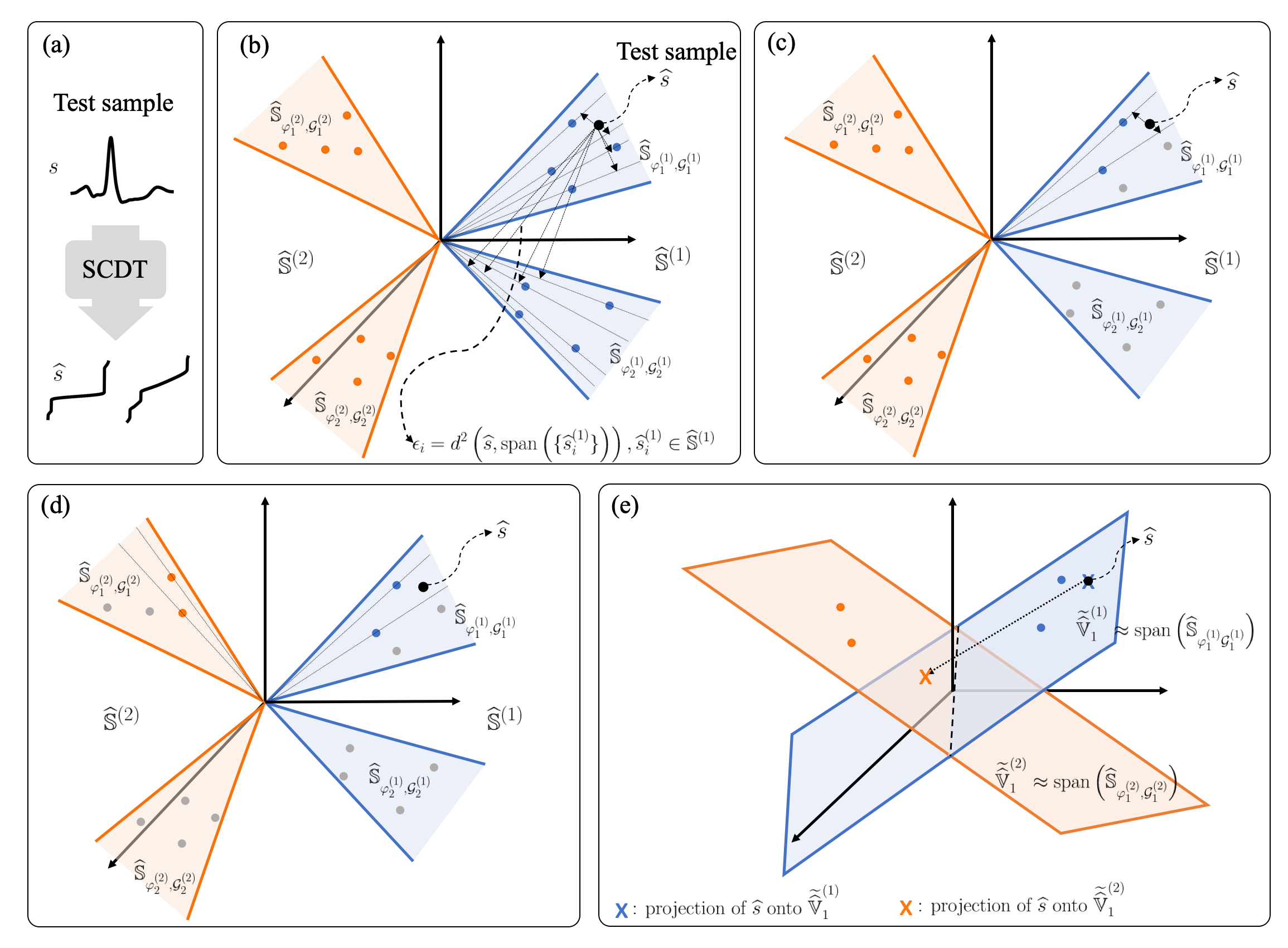
Step 1: We search for the closest training samples to from class based on the distance between and the span of each training sample. First, we sort the elements from the set into such that
| (14) |
where . Then we pick the first elements from the sorted set to form for , which gives the set of closest training samples to from class in the above sense (Fig. 4b-4c). We repeat this step for all other classes (Fig. 4d).
Step 2: Compute by:
| (15) |
which approximates the nearest local subspace from class with respect to . We then predict the unknown class of the test sample by solving eq. (13). Fig. 4e illustrates the second step. Note that similar local subspace classification techniques can be found in the literature [36] [37]. Here, we employ the nearest local subspace search technique in the SCDT domain to exploit the properties of the SCDT that simplify the classification problem described above. Next, we show that the performance of the classifier can further be improved by utilizing the composition property of the SCDT through analytical enrichment of the subspace method.
III-C1 Subspace enrichment
The algorithm outlined above searches for the closest training samples to a given test sample in SCDT domain, and then forms a local subspace using these samples. Inspired by [35, 38], here we adapt the technique to mathematically enrich the ensuing subspace with certain prescribed deformations. Here we enrich in such a way that it will automatically include the samples undergoing certain time deformations. The spanning sets corresponding to certain specific deformations are derived below:
- •
Translation: In case of translation, is given by , where is the translation parameter. Using the composition property of the SCDT, the transform of the translated signal is given by . It implies that the translation applied to the signal along the independent axis results in translation along the dependent axis in SCDT domain. Hence, the spanning set for translation is defined as , where .
- •
Dilation: A time-dilated (scaled) version of a signal is defined as: . The transform of the signal is given by: . An additional spanning set is not required for dilation, as it is inherent in the modeling of the subspace.
- •
Time-warpings other than translation and dilation are also observed in certain classification problems. To include those deformations in the SCDT domain, we approximate the increasing function as:
(16) where, , and
For the set from eq. (15), the spanning set is given by the set , for .
In light of the discussion above, the subspace in eq. (15) can be enriched as follows:
| (17) |
Note that the subspace in (14) can also be enriched in similar manner, i.e. , where , for .
III-C2 Training phase
In the training phase of the algorithm, the subspace corresponding to each of training sample is calculated. The first step is to compute SCDTs for all training samples from class . Then, we take a training sample and orthogonalize to obtain the basis vectors that span the enriched subspace corresponding to that sample. Let be a matrix that contains the basis vectors in its column. We repeat these calculations for all the training samples to form for and etc.
III-C3 Testing phase
The testing algorithm begins with taking SCDT of the test sample to obtain followed by the nearest local subspace search in SCDT domain. In the first step of the algorithm, we estimate the distance of the subspace corresponding to each of the training samples from by:
where denotes norm. Note that is the orthogonal projection matrix onto the space generated by the span of the columns of (computed in the training phase). We then find , a set of closest training samples to the test sample from class , based on the distances . In the next step, we orthogonalize to obtain the basis vectors spanning the local subspace from class with respect to . Let for etc. The unknown class of is then estimated by:
| (18) |
Note that the proposed algorithm requires two parameters and (see eq. (16)) to be tuned prior to the testing phase. We use a validation set split from the training set to estimate the optimum values for these parameters. We then follow the steps of the proposed algorithm outlined above with the validation set for varying and . Parameter values corresponding to the best validation accuracy are chosen to be used in the testing phase. This step is done during the training phase.
III-D Proof-of-concept simulation
To demonstrate the efficacy of the proposed algorithm in solving the classification problem stated in section III-A we performed a simulated experiment. We took six prototype signals shown in Fig. 5 as the templates () corresponding to three different classes (), i.e., each class has two templates (). We then generated a synthetic dataset by applying specific time deformations on the prototype signals as follows:
| (19) |
where and the parameter values used to calculate are randomly chosen from fixed intervals. The dataset was equally split into training and testing sets. The proposed classification method was then trained with a varying number of training samples per class randomly chosen from the training set and evaluated on the testing set. Note that the samples were chosen in such a way that the training set contains an equal number of samples generated from each template. Fig. 5 shows the test accuracy plots with respect to the number of training samples per class. It demonstrates that the proposed method achieves the perfect classification accuracy with few training samples (obtained test accuracy with only training samples per class), while some alternative end-to-end systems (discussed in next section) fail to achieve such performance even with higher number of training data. That means, if the signal classes follow the generative model defined in eq. (9), the proposed method solves the signal classification problem stated in section III-A.


IV Experiments and Results
IV-A Experimental setup
The goal is to evaluate the performance of the proposed generic end-to-end classifier with respect to selected state-of-the-art end-to-end time series classification techniques. The classification performance of the different methods were studied in terms of test accuracy, data efficiency, computational efficiency, and robustness to the out-of-distribution samples. We conducted experiments on several time series data and compared the results against several methods: Multilayer Perceptrons (MLP) [39], 1D Visual Geometry Group (VGG) [39], 1D Residual Network (ResNet) [40] [39], Long Short Term Memory (LSTM) [41] [39], Long Short Term Memory Fully Convolutional Network (LSTM-FCN) [29] [39], and 1-nearest neighbor DTW (1NN-DTW) [24]. For the neural network methods, we used the implementations outlined in [39] without any data augmentation. During the training process, of the training samples were used as the validation set, and the test performance was reported based on the model that had the best validation performance. In case of the 1NN-DTW method, the validation set was used to tune the parameter corresponding to the warping window size. To show the efficacy of the proposed multiple template-based generative model (defined in eq. (9)) over the single template-based model (eq. (8)), we also compared the results against the SCDT-NS classifier [9] proposed earlier.
We followed the training and testing procedures outlined in the previous section for the proposed method. The orthogonalization operations were performed using singular value decomposition (SVD). The left singular vectors obtained by the SVDs were used to construct the matrices and . Following [35], the number of the basis vectors was chosen in such a way that the sum of variances explained by the selected basis vectors captures at least of the total variance explained by all the samples in the sorted set . The SCDTs were computed with respect to a 1D uniform probability density function.
IV-B Datasets
To evaluate the comparative performance of the proposed method with respect to other end-to-end classifiers we selected multiple datasets with signal classes representing well-defined time series events. For example, the accelerometer data plotted in Fig. 6(a) represent particular hand gestures. Similarly, signals shown in Fig. 6(i) represent either normal or abnormal heartbeats. With a focus towards this condition, we identified 10 different time series datasets, 8 of which were downloaded from the UCR time series classification archive [42]. Some example signals from these datasets are shown in Fig. 6. Details about the datasets are given below:
- •
GesturePebbleZ2 [43]: Accelerometer data collected using Pebble smart watch from 4 different persons performing 6 hand gestures. (classes: 6, train samples: per class, test samples: per class).
- •
InsectEPGRegularTrain [44]: Contains electrical penetration graph (EPG) data which capture voltage changes of the electrical circuit that connects insects and their food source. (classes: 2, train samples: per class, test samples: per class).
- •
PLAID: Plug Load Appliance Identification Dataset [45]. The data are intended for load identification research using transient voltage/current measurements from 11 different appliance types. (classes: 11, train samples: per class, test samples: per class).
- •
UWaveGestureLibraryAll [46]: A set of eight simple gestures generated from accelerometers using Wii remote. (classes: 8, train samples: per class, test samples: per class).
- •
Wafer [47]: A collection of inline process control measurements recorded from various sensors during the processing of silicon wafers. The two classes are normal and abnormal, with a significant class imbalance. Hence, a subset of the original dataset is used to ensure the class balance. (classes: 2, train samples: per class, test samples: per class).
- •
StarLightCurves [48]: Collection of time series signals representing the brightness of celestial objects as a function of time. (classes: 3, train samples: per class, test samples: per class).
- •
TwoPatterns [49]: A simulated dataset (classes: 4, train samples: per class, test samples: per class).
- •
ECG5000 [42]: A subset of BIDMC Congestive Heart Failure Database (CHFDB) downloaded from PhysioNet. With a purpose of evaluating the methods trained with a large set, we interchanged the train and test sets of the original dataset. (classes: 2, train samples: per class, test samples: per class).
- •
ECG (MLII) [50]: A subset of a publicly available dataset reported in [51]. The ECG signals were collected from the PhysioNet MIT-BIH Arrythmia database [52]. A method described in [53] was used to segment the heartbeats from the ECG fragments. (classes: 3, train samples: per class, test samples: per class).
- •
Connectionist Bench (Sonar, Mines vs. Rocks) [54] [55]: This dataset contains energy patterns (with respect to frequency bands) of the signals obtained by bouncing sonar signals off a metal cylinder and some rocks at various angles and under various conditions. (classes: 2, train samples: per class, test samples: ).
In addition to the datasets listed above, we have used another dataset where time series events are not well-defined as an example where the proposed method is not expected to work well. We have used the gearbox fault diagnosis data [56], a collection of vibration signals recorded by using SpectraQuest’s Gearbox Fault Diagnostics Simulator. The dataset was recorded in two different scenarios: 1) healthy and 2) broken tooth conditions.

IV-C Test accuracy
| Dataset | MLP | 1D-VGG | 1D-ResNet | LSTM | LSTM-FCN | SCDT-NS | 1NN-DTW | Proposed |
| GesturePebbleZ2 | 83.92 | 48.99 | 63.23 | 60.19 | 85.82 | 81.64 | 94.94 | 94.30 |
| InsectEPGRegularTrain | 80.92 | 82.07 | 50.58 | 57.05 | 59.95 | 73.43 | 82.61 | 90.82 |
| PLAID | 39.65 | 19.35 | 29.81 | 26.35 | 39.57 | 58.29 | 73.56 | 70.95 |
| UWaveGestureLibraryAll | 94.74 | 96.42 | 42.86 | 30.72 | 94.16 | 90.4 | 94.22 | 94.95 |
| Wafer | 68.69 | 94.03 | 53.66 | 51.36 | 86.70 | 92.75 | 98.16 | 95.60 |
| StarLightCurves | 75.85 | 70.0 | 56.53 | 60.54 | 74.38 | 77.4 | 83.80 | 84.2 |
| TwoPatterns | 88.12 | 95.15 | 87.42 | 80.62 | 98.47 | 95.15 | 99.90 | 99.92 |
| ECG5000 | 98.9 | 98.92 | 98.92 | 98.36 | 98.76 | 93.4 | 99.2 | 97.6 |
| ECG (MLII) | 33.33 | 33.33 | 56.55 | 44.20 | 66.42 | 56.67 | 45.67 | 68.83 |
| Sonar | 68.36 | 80.57 | 53.85 | 53.85 | 53.85 | 61.54 | 76.92 | 78.85 |
| Win | 0 | 2 | 0 | 0 | 0 | 0 | 4 | 4 |
| AVG arithmetic ranking | 4.6 | 4.3 | 6.1 | 7.0 | 4.7 | 4.7 | 2.2 | 2.2 |
| AVG geometric ranking | 4.46 | 3.38 | 5.73 | 6.94 | 4.4 | 4.48 | 1.85 | 1.84 |
| MPCE | 0.084 | 0.072 | 0.123 | 0.128 | 0.079 | 0.071 | 0.049 | 0.038 |
To demonstrate the efficacy of the proposed method as a generic classifier, we applied it to the datasets listed above and compared the test accuracies against the aforementioned end-to-end classification methods. Table II shows the results and a comprehensive comparison with five neural network-based classifiers, 1NN-DTW, and SCDT-NS. The results reported in the table show that in most of the datasets (8 out of 10), the proposed method outperformed the deep learning methods and provided competitive test accuracy with respect to 1NN-DTW. The average arithmetic and geometric rankings also demonstrate the efficacy of the proposed method as a generic end-to-end technique to classify segmentable time series events.
Besides test accuracy and rank-based statistics, we also calculated mean per class error (MPCE) for each method. This metric was proposed in [27] to evaluate the performance of a generic classifier on multiple datasets. MPCE is defined as the arithmetic mean of the per class error (PCE) which is calculated for -th model on -th dataset as: . Here is the error rate of -th model on -th dataset, and is the total number of classes present in -th dataset. MPCE for the corresponding model is given by,
where is the total number of datasets used in the experiment. The MPCE values reported in Table II indicate that the proposed method generates the least expected error rate per class across all the datasets in comparison to other classifiers.
IV-D Data efficiency
To show the data efficiency of the proposed method, we set up an experiment where we trained the models with a varying number of training samples per class. For a training split of a particular size, its samples were randomly drawn from the original training set, and the experiments for this particular size were repeated 10 times. Fig. 7 shows average accuracies with respect to the number of training samples per class for two datasets: UWaveGestureLibraryAll and TwoPatterns. The standard deviation for each split is also shown using the error bar. The plots illustrate that the proposed method achieves higher accuracy than the deep learning methods with fewer training samples. Similar results can be seen in other datasets as well (see Appendix B in supplementary materials).


IV-E Computational efficiency
The proposed classification technique is not only effective in classifying time series events but also computationally very efficient. Fig. 8 shows the computational complexity plots of the proposed method and 1NN-DTW as a function of number of training samples per class for TwoPatterns dataset. It demonstrates that the proposed classifier requires less CPU operations in comparison to 1NN-DTW. Fig. 9 (upper panel) plots the average time (in seconds) required during the training phase as a function of accuracy for each method. It illustrates that all the alternative end-to-end solutions require greater number of computations to train the models with respect to the proposed solution to achieve same level of accuracy. Despite the fact that our method searches for -closest training samples for a given test signal, it still provides competitive performance as shown in Fig. 9 (lower panel) in terms of test time in comparison to deep learning-based methods. The plots of the average time (in seconds) taken by the classification methods to test a signal from TwoPatterns dataset show that the test time of the proposed method is close to the neural network-based classifiers, while 1NN-DTW is highly expensive in terms of computation during testing phase. Note that the SCDT is currently implemented with for loops in python, which is less than ideal in terms of execution time. A compiled language (e.g. C, C++) would execute for loops much faster.


IV-F Robust to out-of-distribution samples
To demonstrate the robustness to out-of-distribution examples, we adopted a similar concept used in [9]. We generated a synthetic dataset by applying time deformations defined in eq. (19) on three prototype signals: a Gabor wave, an apodized sawtooth wave, and an apodized square wave (shown in the top row of Fig. 7). Note that we used a single template per class to generate data for maintaining a simple experimental setup. We varied the magnitude of the confounding factors (i.e., the parameters used to calculate ) to generate different distributions for training and testing sets. The ‘in-distribution’ set used during the training process consisted of signals with parameter values chosen randomly from smaller intervals with respect to the ‘out-distribution’ (testing) set. Table III shows the list of the parameters of interest for the ‘out-of-distribution’ experiment. The intervals (from which the parameter values were chosen) corresponding to the training and testing sets are also given in the table. Fig. 10 shows test accuracies with respect to the number of training samples per class for the comparing methods. The plot shows that the proposed method significantly outperforms other end-to-end solutions with very few training samples. Meaning, the proposed classification technique provides the best classification result if the test signal belongs to the ‘out-distribution’ set in the above sense but follows the generative model discussed in the previous section.
| Parameter | Train | Test |

IV-G A dataset that does not follow generative model
As described in IV-B, the proposed method performs well if the time series data is well segmented, i.e. contains events with well-defined start and end points. There are examples of signal classification problems where data do not follow these conditions. One such example is the gearbox fault diagnosis dataset [56], where vibration signals are used to detect a faulty gearbox. Fig. 11(a) shows that the vibration signals do not possess segmentable time series events. Hence, the proposed method is not suitable for classifying raw gearbox vibration data, as shown in the table in Fig. 11. However, we can transform each time series to frequency domain using the Fourier transform [57], where signals of finite length are necessarily band limited (and thus have a beginning and end in frequency domain). As expected the proposed method performs better when applied to the frequency domain signals shown in Fig. 11(b).

| Method | Time domain | Frequency domain |
| MLP | 55.67 | 90.45 |
| 1D-VGG | 50.77 | 56.02 |
| 1D-ResNet | 71.5 | 50.0 |
| LSTM | 57.32 | 72.35 |
| LSTM-FCN | 76.5 | 90.92 |
| SCDT-NS | 52.75 | 91.5 |
| 1NN-DTW | 75.75 | 93.5 |
| Proposed | 57.25 | 89.5 |
V Discussion
Classification test accuracies, rank-based statistics, and MPCE reported in Table II across 10 different time series datasets suggest that the proposed method is a very good generic end-to-end signal classification model for time series containing segmented events. Moreover, Fig. 7 shows that the proposed method can achieve high accuracy with few training samples. The computational efficiency of the proposed classifier is also demonstrated in figures 8 and 9 in terms of CPU operations, and average training and testing time with respect to other end-to-end classifiers. It is also evident from Table II that the proposed method outperforms the SCDT-NS classifier [9] which uses a single template-based generative model.
Another compelling property of the proposed method is the robustness to out-of-distribution samples since it generalizes to samples outside the known distribution when the signal classes conform to the specific generative model. Plots in Fig. 10 show that other methods fail to achieve good performance under the out-of-distribution setup, whereas the proposed method achieves perfect test accuracy with very few training samples ( per class). The reason behind the robustness to the out-of-distribution setup is that the proposed method is capable of learning the underlying data model, more specifically, the types of unknown deformations present in the signals. It can then successfully classify an unknown signal in presence of such deformations but with different magnitudes.
The main assumption of the proposed method is that the dataset needs to conform to the underlying generative model proposed earlier. Specifically, we showed above that the method works best when the time series (signal) being classified contains segmented events with finite duration. Fig. 11 shows an example where raw signals (from a gearbox vibration experimental setup) do not possess well-defined time series events of finite duration. Hence, the proposed method performs poorly in classifying those signals. However, the same signals in frequency domain seem to fit the generative model better and the proposed method performs better in classifying the gearbox data in frequency domain.
To summarize, this paper presents a new idea of representing segmented signal data using a generative model such that signals from a particular class can be considered as observations of a set of unknown templates under some unknown deformations. Under this assumption, we formulated a classification problem for segmented signal classes. Then we showed that if the data follow the proposed generative model, a simple solution can be devised by searching nearest local subspace in SCDT domain. Through extensive experiments, we demonstrated that the proposed solution is effective in classifying unknown signals, computationally very cheap, data efficient, and robust to out-of-distribution samples.
VI Conclusion
This paper introduced a new end-to-end signal classification method based on a recently developed signal transform. First, we formulated the problem statement based on a multiple template-based generative model observed under unknown deformations. Then, we proposed an end-to-end solution to the problem by employing a nearest local subspace search algorithm in SCDT domain. Although the problem statement and solution are based on the assumption that signals are observations of templates under confounding deformations, knowledge of these templates or confound deformations is not required. The model was demonstrated to achieve high test accuracy across multiple time series datasets. Several experiments show that the proposed method not only outperforms the state-of-the-art deep learning based end-to-end methods but also is data efficient and robust to out-of-distribution examples. Moreover, it provides competitive performance in classifying segmented time series events with respect to 1NN-DTW with very cheap computational complexity. We note that the approach assumes that the data being classified follows a certain generative model. Namely, each time series should contain an event with finite support, that is, with beginning and end within the recorded time series. We showed that for signal classes that do not contain events of finite duration the approach is less effective. Future work will include exploring ways to extend this method to classify time series events that are not readily segmentable.
Acknowledgements
This work was supported in part by NIH grant GM130825.
References
- [1] Imaging and data science lab, “PyTransKit,” https://github.com/rohdelab/PyTransKit.
- [2] O. D. Lara and M. A. Labrador, “A survey on human activity recognition using wearable sensors,” IEEE communications surveys & tutorials, vol. 15, no. 3, pp. 1192–1209, 2012.
- [3] S. K. Berkaya, A. K. Uysal, E. S. Gunal, S. Ergin, S. G., and M. B. Gulmezoglu, “A survey on ECG analysis,” Biomedical Signal Processing and Control, vol. 43, pp. 216–235, 2018.
- [4] A. Subasi and M. I. Gursoy, “EEG signal classification using PCA, ICA, LDA and support vector machines,” Expert systems with applications, vol. 37, no. 12, pp. 8659–8666, 2010.
- [5] A. Fehske, J. Gaeddert, and J. H. Reed, “A new approach to signal classification using spectral correlation and neural networks,” in First IEEE International Symposium on New Frontiers in Dynamic Spectrum Access Networks, 2005. DySPAN 2005. IEEE, 2005, pp. 144–150.
- [6] O. Abdeljaber, O. Avci, M. S. Kiranyaz, B. Boashash, H. Sodano, and D. J. Inman, “1-D CNNs for structural damage detection: Verification on a structural health monitoring benchmark data,” Neurocomputing, vol. 275, pp. 1308–1317, 2018.
- [7] R. Zhao, R. Yan, Z. Chen, K. Mao, P. Wang, and R. X. Gao, “Deep learning and its applications to machine health monitoring,” Mechanical Systems and Signal Processing, vol. 115, pp. 213–237, 2019.
- [8] C. Lu, T. Lee, and C. Chiu, “Financial time series forecasting using independent component analysis and support vector regression,” Decision support systems, vol. 47, no. 2, pp. 115–125, 2009.
- [9] A. H. M. Rubaiyat, M. Shifat-E-Rabbi, Y. Zhuang, S. Li, and G. K. Rohde, “Nearest subspace search in the signed cumulative distribution transform space for 1d signal classification,” in ICASSP 2022-2022 IEEE International Conference on Acoustics, Speech and Signal Processing (ICASSP). IEEE, 2022, pp. 3508–3512.
- [10] A. Aldroubi, R. D. Martin, I. Medri, G. K. Rohde, and S. Thareja, “The signed cumulative distribution transform for 1-D signal analysis and classification,” Foundations of Data Science, 2022.
- [11] A. Nanopoulos, R. Alcock, and Y. Manolopoulos, “Feature-based classification of time-series data,” International Journal of Computer Research, vol. 10, no. 3, pp. 49–61, 2001.
- [12] A. Bagnall, J. Lines, A. Bostrom, J. Large, and E. Keogh, “The great time series classification bake off: a review and experimental evaluation of recent algorithmic advances,” Data mining and knowledge discovery, vol. 31, no. 3, pp. 606–660, 2017.
- [13] B. D. Fulcher and N. S. Jones, “Highly comparative feature-based time-series classification,” IEEE Transactions on Knowledge and Data Engineering, vol. 26, no. 12, pp. 3026–3037, 2014.
- [14] H. I. Fawaz, G. Forestier, J. Weber, L. Idoumghar, and P.-A. Muller, “Deep learning for time series classification: a review,” Data mining and knowledge discovery, vol. 33, no. 4, pp. 917–963, 2019.
- [15] J. Wang, Y. Chen, S. Hao, X. Peng, and L. Hu, “Deep learning for sensor-based activity recognition: A survey,” Pattern Recognition Letters, vol. 119, pp. 3–11, 2019.
- [16] M. M. Al Rahhal, Y. Bazi, H. AlHichri, N. Alajlan, F. Melgani, and R. R. Yager, “Deep learning approach for active classification of electrocardiogram signals,” Information Sciences, vol. 345, pp. 340–354, 2016.
- [17] M. G. Baydogan, G. Runger, and E. Tuv, “A bag-of-features framework to classify time series,” IEEE transactions on pattern analysis and machine intelligence, vol. 35, no. 11, pp. 2796–2802, 2013.
- [18] A. Bagnall, J. Lines, J. Hills, and A. Bostrom, “Time-series classification with COTE: the collective of transformation-based ensembles,” IEEE Transactions on Knowledge and Data Engineering, vol. 27, no. 9, pp. 2522–2535, 2015.
- [19] J. Lines, S. Taylor, and A. Bagnall, “Time series classification with HIVE-COTE: The hierarchical vote collective of transformation-based ensembles,” ACM Transactions on Knowledge Discovery from Data, vol. 12, no. 5, 2018.
- [20] H. Deng, G. Runger, E. Tuv, and M. Vladimir, “A time series forest for classification and feature extraction,” Information Sciences, vol. 239, pp. 142–153, 2013.
- [21] A. Abanda, U. Mori, and J. A. Lozano, “A review on distance based time series classification,” Data Mining and Knowledge Discovery, vol. 33, no. 2, pp. 378–412, 2019.
- [22] J. Lines and A. Bagnall, “Time series classification with ensembles of elastic distance measures,” Data Mining and Knowledge Discovery, vol. 29, no. 3, pp. 565–592, 2015.
- [23] D. J. Berndt and J. Clifford, “Using dynamic time warping to find patterns in time series.” in KDD workshop, vol. 10, no. 16. Seattle, WA, USA:, 1994, pp. 359–370.
- [24] X. Xi, E. Keogh, C. Shelton, L. Wei, and C. A. Ratanamahatana, “Fast time series classification using numerosity reduction,” in Proceedings of the 23rd international conference on Machine learning, 2006, pp. 1033–1040.
- [25] Y. Zheng, Q. Liu, E. Chen, Y. Ge, and J. L. Zhao, “Time series classification using multi-channels deep convolutional neural networks,” in International conference on web-age information management. Springer, 2014, pp. 298–310.
- [26] B. Zhao, H. Lu, S. Chen, J. Liu, and D. Wu, “Convolutional neural networks for time series classification,” Journal of Systems Engineering and Electronics, vol. 28, no. 1, pp. 162–169, 2017.
- [27] Z. Wang, W. Yan, and T. Oates, “Time series classification from scratch with deep neural networks: A strong baseline,” in 2017 International joint conference on neural networks (IJCNN). IEEE, 2017, pp. 1578–1585.
- [28] Z. Cui, W. Chen, and Y. Chen, “Multi-scale convolutional neural networks for time series classification,” arXiv preprint arXiv:1603.06995, 2016.
- [29] F. Karim, S. Majumdar, H. Darabi, and S. Chen, “LSTM fully convolutional networks for time series classification,” IEEE access, vol. 6, pp. 1662–1669, 2017.
- [30] S. Kolouri, S. R. Park, M. Thorpe, D. Slepcev, and G. K. Rohde, “Optimal mass transport: Signal processing and machine-learning applications,” IEEE signal processing magazine, vol. 34, no. 4, pp. 43–59, 2017.
- [31] S. R. Park, S. Kolouri, S. Kundu, and G. K. Rohde, “The cumulative distribution transform and linear pattern recognition,” Applied and computational harmonic analysis, vol. 45, pp. 616–641, 2018.
- [32] W. Wang, D. Slepčev, S. Basu, J. A. Ozolek, and G. K. Rohde, “A linear optimal transportation framework for quantifying and visualizing variations in sets of images,” International journal of computer vision, vol. 101, no. 2, pp. 254–269, 2013.
- [33] A. H. M. Rubaiyat, K. M. Hallam, J. M. Nichols, M. N. Hutchinson, S. Li, and G. K. Rohde, “Parametric signal estimation using the cumulative distribution transform,” IEEE Transactions on Signal Processing, vol. 68, pp. 3312–3324, 2020.
- [34] H. L. Royden and P. Fitzpatrick, Real analysis. Macmillan New York, 1988, vol. 32.
- [35] M. Shifat-E-Rabbi, X. Yin, A. H. M. Rubaiyat, S. Li, S. Kolouri, A. Aldroubi, J. M. Nichols, and G. K. Rohde, “Radon cumulative distribution transform subspace modeling for image classification,” Journal of Mathematical Imaging and Vision, pp. 1–19, 2021.
- [36] J. Laaksonen, “Local subspace classifier,” in International Conference on Artificial Neural Networks. Springer, 1997, pp. 637–642.
- [37] H. Cevikalp, D. Larlus, M. Douze, and F. Jurie, “Local subspace classifiers: Linear and nonlinear approaches,” in 2007 IEEE Workshop on Machine Learning for Signal Processing. IEEE, 2007, pp. 57–62.
- [38] M. S. E. Rabbi, Y. Zhuang, S. Li, A. H. M. Rubaiyat, X. Yin, and G. K. Rohde, “Invariance encoding in sliced-Wasserstein space for image classification with limited training data,” arXiv preprint arXiv:2201.02980, 2022.
- [39] B. K. Iwana and S. Uchida, “An empirical survey of data augmentation for time series classification with neural networks,” Plos one, vol. 16, no. 7, p. e0254841, 2021.
- [40] H. I. Fawaz, G. Forestier, J. Weber, L. Idoumghar, and P.-A. Muller, “Data augmentation using synthetic data for time series classification with deep residual networks,” arXiv preprint arXiv:1808.02455, 2018.
- [41] S. Hochreiter and J. Schmidhuber, “Long short-term memory,” Neural computation, vol. 9, no. 8, pp. 1735–1780, 1997.
- [42] H. A. Dau, E. Keogh, K. Kamgar, C.-C. M. Yeh, Y. Zhu, S. Gharghabi, C. A. Ratanamahatana, Yanping, B. Hu, N. Begum, A. Bagnall, A. Mueen, G. Batista, and Hexagon-ML, “The UCR time series classification archive,” October 2018, https://www.cs.ucr.edu/~eamonn/time\_series\_data\_2018/.
- [43] A. Mezari and I. Maglogiannis, “Gesture recognition using symbolic aggregate approximation and dynamic time warping on motion data,” in Proceedings of the 11th EAI International Conference on Pervasive Computing Technologies for Healthcare, 2017, pp. 342–347.
- [44] D. S. Willett, J. George, N. S. Willett, L. L. Stelinski, and S. L. Lapointe, “Machine learning for characterization of insect vector feeding,” PLoS computational biology, vol. 12, no. 11, p. e1005158, 2016.
- [45] J. Gao, S. Giri, E. C. Kara, and M. Bergés, “PLAID: a public dataset of high-resoultion electrical appliance measurements for load identification research: demo abstract,” in proceedings of the 1st ACM Conference on Embedded Systems for Energy-Efficient Buildings, 2014, pp. 198–199.
- [46] J. Liu, L. Zhong, J. Wickramasuriya, and V. Vasudevan, “uWave: Accelerometer-based personalized gesture recognition and its applications,” Pervasive and Mobile Computing, vol. 5, no. 6, pp. 657–675, 2009.
- [47] R. T. Olszewski, Generalized feature extraction for structural pattern recognition in time-series data. Carnegie Mellon University, 2001.
- [48] U. Rebbapragada, P. Protopapas, C. E. Brodley, and C. Alcock, “Finding anomalous periodic time series,” Machine learning, vol. 74, no. 3, pp. 281–313, 2009.
- [49] P. Geurts, “Contributions to decision tree induction: bias/variance tradeoff and time series classification,” Ph.D. dissertation, ULiège-University of Liège, 2002.
- [50] P. Pławiak, “ECG signals (744 fragments),” 2017.
- [51] P. Pławiak, “Novel genetic ensembles of classifiers applied to myocardium dysfunction recognition based on ECG signals,” Swarm and evolutionary computation, vol. 39, pp. 192–208, 2018.
- [52] S. Mousavi and F. Afghah, “Inter-and intra-patient ECG heartbeat classification for arrhythmia detection: a sequence to sequence deep learning approach,” in ICASSP 2019-2019 IEEE International Conference on Acoustics, Speech and Signal Processing (ICASSP). IEEE, 2019, pp. 1308–1312.
- [53] M. M. Bassiouni, E. A. El-Dahshan, W. Khalefa, and A. M. Salem, “Intelligent hybrid approaches for human ECG signals identification,” Signal, Image and Video Processing, vol. 12, no. 5, pp. 941–949, 2018.
- [54] D. Dua and C. Graff, “UCI machine learning repository,” 2017. [Online]. Available: http://archive.ics.uci.edu/ml
- [55] R. P. Gorman and T. J. Sejnowski, “Analysis of hidden units in a layered network trained to classify sonar targets,” Neural networks, vol. 1, no. 1, pp. 75–89, 1988.
- [56] N. R. E. Laboratory, “Gearbox fault diagnosis data [data set],” 2018, http://data.openei.org/submissions/623.
- [57] R. N. Bracewell and R. N. Bracewell, The Fourier transform and its applications. McGraw-hill New York, 1986, vol. 31999.