Acknowledgment

Spectral Analysis and Preconditioned Iterative Solvers for Large Structured Linear Systems

Nikos Barakitis

ATHENS UNIVERSITY OF ECONOMICS AND BUSINESS
SCHOOL OF INFORMATION SCIENCES AND TECHNOLOGY
DEPARTMENT OF INFORMATICS

Acknowledgment

I would firstly like to thank my supervisor, Associate Professor Paris Vassalos and my advisor, Professor Stefano Serra-Capizzano, for the unlimited help and support they offered to me during my studies. I would also like to thank Emeritus Professor Evaggelos Mageirou for his throughout invaluable help and guidance, and my advisor Professor Dimitrios Noutsos for being member of the advising commitee and generously sharing ideas with the team.

I would also like to thank my collaborator researchers, Sven-Erik Erkstrom and Paola Ferrari for the fruitful collaboration we had, and their patience.

Finally, I would like to thank Associate Professor Stavros Toumpis and Professor Panagiotis Katerinis for their attitude toward me at several moments which helped me to build my self confidence and made me to believe that the completion of this dissertation could be feasible.

Thank you,
Nikos Barakitis, Athens 2021.

Introduction

The use of iterative methods for solving large structured linear systems has been of interest for more than half a century, and the development of the field has gone together with the improvement of computer systems. In fact, the solution of a large linear system of the form

\displaystyle Ax=b,

(1)

where the size of $A$ is $n\times n$ and $b$ is a column vector of size $n$ , is often the central and most time- and storage-consuming part of the computation.

Iterative methods for solving linear systems first appeared in the works of Gauss, Seidel, and Jacobi in the 19-th century, with further progress in these methods being made in the first half of the 20-th century. These methods are typically referred to as stationary, as opposed to the other classes of iterative techniques that appeared later and relied on solution searches in Krylov subspaces. For the latter methods, the story began in 1952 with the development of the conjugate gradient (CG) method [30]. This method was proposed for solving symmetric and positive-definite linear systems. Initially, it was considered a direct method, because it was proved analytically to reach the exact solution in at most $n$ steps, or actually in as many steps as the number of distinct eigenvalues of the coefficient matrix. However, in practice, owing to the limited accuracy of floating-point arithmetic, especially in presence of ill-conditioning the method requires more iterations than expected for a satisfactory approximation of the solution. Besides this, when considered as a direct method, it required more arithmetic operations than the Gauss elimination. This method has remained out of interest for two decades. As applications required larger linear systems to be solved, the poor computational escalation of direct methods was overshadowed by the rapid improvement of computers and the evolution of computational methods.

This attitude regarding CG changed in the 70s following a publication from J. Reid [58]. Thereafter, it became clear that for well-conditioned systems, the number of steps that the CG requires to reach the solution with a given accuracy is independent of the size of the system. This work brought Krylov methods back into the focus of the research community. The list of Krylov methods, limited until then, was enriched with methods for non-definite symmetric systems [e.g., the minimum residual method (MINRES) [51]] and methods for non-symmetric systems [e.g., the generalised minimum residual method (GMRES) [61]].

Published by O. Axelson and G. Lindskog in 1986 [2]. Since then, the paper has been included in the references of almost every work relating to the solution of linear systems using iterative Krylov-subspace-theory based methods. In this study, it was proved that the efficiency of the preconditioned CG method depends on the clustering of the eigenvalues of the preconditioned matrix, which are clustered at $(1)$ and yet certainly far from zero. The notion of eigenvalue clustering will be defined later: Hereafter, preconditioning was officially upgraded to the first research target in the field numerical solution of linear systems.¹¹ 1 It must be mentioned here that for methods such as the Generalized Minimum Residual method, applied to non-symmetric systems, the eigenvalue distribution may not exactly describe the convergence[19]. However, in every case, a clustered spectrum and a minimal eigenvalue far from zero ensure fast convergence of the method..

Preconditioning of a linear system refers to the replacement of the system (1) with

		$\displaystyle M^{-1}Ax=M^{-1}b,$
		$\displaystyle M_{1}^{-1}AM_{2}^{-1}y=M_{1}^{-1}b,\quad x=M_{1}^{-1}y,$
		$\displaystyle AM^{-1}y=b,\quad x=M^{-1}y,$

for left, split, and right preconditioning, respectively. In each case, the preconditioned matrix $M^{-1}A,\>M_{1}^{-1}AM_{2}^{-1},\>AM^{-1}$ has a better condition number and superior spectral properties to the original one. For preconditioning to be feasible, the preconditioner must have two somewhat contradictory properties:

•

The preconditioned system must be easily solvable.
•

The determination and the application of the preconditioner must be easy.

The first property suggests that the preconditioner must be fairly close to the coefficient matrix of the system; however, this is generally difficult to solve and contradicts with the second property. To conclude, the next phrase, taken from [60], summarises a view widely adopted in the research community:

”Finding a good preconditioner to solve a given sparse linear system is often viewed as a combination of art and science.”

In general, two classes of preconditioning techniques are available. The first includes purely algebraic methods that use only the information contained in the coefficient matrix. Such methods are typically based on some type of incomplete factorisation or some type of sparse approximate inverse of the coefficient matrix [6, 60]. These methods achieve reasonable efficiency for a wide range of problems; however, they might not be the optimal choice for any one particular problem. The other class of methods, primarily applicable to problems arising from PDEs, involves the design of algorithms that are problem-specific. Such methods might be optimal for any specific problem; however, they require complete knowledge of the problem in advance, especially from a spectral point of view. In these methods, the preconditioners are selected by specific classes of matrices; furthermore, for their construction, a detailed spectral analysis of the coefficient matrix is required.

In the first part of this thesis, preconditioning strategies to solve (using Krylov subspace methods) linear systems arising from two specific problems are proposed. In the first problems, the coefficient matrix of the system emerges as an analytic function of a real Toeplitz matrix. This strategy utilises symmetrisation and preconditioning of the coefficient matrix. Preconditioners are selected from matrix algebras according to the spectral properties of the symmetrised coefficient matrix sequence. The properties of the matrix sequence are extensively analyzed. The second class of problems involves the numerical solution of partial differential equations with a fractional derivative order. These problems have been thoroughly investigated in recent years; however, a new category of preconditioners is here proposed. The new class of preconditioners exhibits optimal behaviour in relation to the proposals given so far in the literature, especially in dimensions of more than one. This behaviour is theoretically confirmed by the numerical results.

The first part of this thesis is structured as follows: The first chapter introduces all the necessary definitions and summarises the theory used to analyse the spectral properties of the coefficient matrix sequences. In the second chapter, the problem of symmetrising the large matrices that emerge as analytic functions of real Toeplitz matrices is considered. In the third chapter, is studied the numerical solution of fractional partial differential equations.

In the second part the numerical solution of a problem arising in finance is considered. In detail a numerical technique based again on an iterative algorithm is used for pricing an American put option. A put option is a financial derivative that gives the right (but not the obligation) to the holder to sell an asset for a pre-specified price $K$ , the exercise or strike price. The other party, the writer of the option, must accept the sale for the exercise price regardless of the current price $S$ of the asset at the time of exercise. The right can be exercised either only on the pre-determined expiry or maturity date in case of the European put option, or any day up to the pre-determined expiry date in the American put option. In any case, because the holder does not have an obligation to sell, the right will be exercised only if the current price $S$ is lower than $K$ . In this case, the profit of the seller will be $K-S$ .

Since they were invented, such rights have been traded on the market as assets; therefore, a fair pricing process is needed. In a viable, where arbitrage opportunities are not allowed market model, the value of such a right at time $t$ before the maturity date should be equal to the price of a portfolio which has the same expected payoff value as the option at the exercise date at time $t$ . For the European put option, it has been shown that the fair price $V(S,t)$ at time $t$ before the maturity date and for asset price $S$ must satisfy the Black–Scholes equation. At maturity time $T$ , the value $V(S,T)$ of the option must be equal to the payoff function.

Despite the similarities between the two types of put options, the American put, compared with the European put, gives its holder the additional advantage in that it can be exercised any day before the maturity date, thereby offering them additional profit opportunities. It is fair, therefore, that this privilege should be taken into account in the pricing process of the option. Moreover, according to the process in which the price of the option at time $t$ is equal to the price of a portfolio (with the same expected payoff on the exercise day) at time $t$ , all the possible exercise times between should be taken into account. Although many of the characteristics of the value function of an American put option have been extensively analysed the pricing of such an options is a problem that has not yet been solved analytically.

Taking advantage of the known characteristics of the optimal value function, the iterative algorithm presented here, which utilises the principles of dynamic programming, iteratively improves exercise policies, obtains monotonically increasing value functions and converges quadratically under reasonable assumptions. The exact meaning of a policy will be defined in relevant chapter.

This thesis is based on the published papers [12] and [36], an accepted for publication [3] and an under progress work.

Part I Spectral Analysis and Preconditioned Iterative Solvers for Large Structured Linear Systems

Chapter 1 Generalized Locally Toeplitz Matrix Sequences

As mentioned in the introduction, the preconditioners for a large class of linear systems are constructed following analysis of the properties of the initial problem, which relate to the effective application of iterative methods. These properties include the condition number, asymptotic distribution of the eigenvalues, and singular values of the system coefficient matrix sequence. The theory used here to study matrix sequences is that of generalised locally Toeplitz (GLT) matrix sequences. This theory unifies, and essentially provides all the tools needed to study the asymptotic behaviour of the eigenvalues and singular values of matrix sequences obtained from the discretisation of differential or integral equations (as well as more besides).

The theory was introduced in Paollo Tilli’s paper on locally Toeplitz (LT) matrix sequences [71]. The idea was further developed by Stefano Serra-Capizzano in [67, 68] and also in a series of subsequent papers. A complete presentation of the theory can be found in [15, 16]. In the following, we define a matrix sequence as a sequence of the form $\{A_{n}\}_{n}$ , where $A_{n}\in\;\mathbb{C}^{n\times n}$ and $n\in\mathbb{N}$ . The abbreviations LT and GLT matrix sequences denote locally Toeplitz and generalised locally Toeplitz matrix sequences, respectively.

1.1 Singular Value, Eigenvalue Distribution, and Clustering of Matrix Sequences

Definition 1.1.

Let $f:D\subset\mathbb{R}^{n}\to\mathbb{C}$ be a function and $\{A_{n}\}_{n}$ be a matrix sequence. $\{A_{n}\}_{n}$ has an eigenvalue distribution described by $f$ , and we write $\{A_{n}\}_{n}\sim_{\lambda}f$ if

\lim_{n\to\infty}\frac{1}{n}\sum_{j=1}^{n}F(\lambda_{j}(A_{n}))=\frac{1}{\mu(D)}\int_{D}F(f(x))dx,\quad\forall F\in C_{c}(\mathbb{C}),

(1.1)

where $\mu(D)$ is the Lebesgue measure of $D$ , $\mu(D)\in(0,\infty)$ and $C_{c}(\mathbb{C})$ is the set of all continuous functions defined on $\mathbb{C}$ , whose support¹¹ 1 The support of a function $f$ , denoted by $suppf$ , is the set $\overline{\{x|f(x)\neq 0\}}$ is a closed and bounded subset of $\mathbb{C}$ .

We say that $\{A_{n}\}_{n}$ has a singular value distribution described by $f$ , and we write $\{A_{n}\}_{n}\sim_{\sigma}f$ if

\lim_{n\to\infty}\frac{1}{n}\sum_{j=1}^{n}F(\sigma_{j}(A_{n}))=\frac{1}{\mu(D)}\int_{D}F(|f(x)|)dx,\quad\forall F\in C_{c}(\mathbb{R}),

(1.2)

where $\mu(D)\in(0,\infty)$ and $C_{c}(\mathbb{R})$ is the set of all continuous functions defined on $\mathbb{R}$ , whose support is a closed and bounded subset of $\mathbb{R}$ .

Intuitively speaking, if the matrix sequence $\{A_{n}\}_{n}$ has an eigenvalue distribution described by $f:D\subset\mathbb{R}^{n}\to\mathbb{C}$ , then under the condition that $f$ is continuous $a.e.$ ²² 2 a.e.: almost anywhere. If $f$ is not continuous over a set of zero measures at most, then $f$ is continuous almost anywhere., the properly rearranged eigenvalues are close to a sampling of $f$ on an equispaced grid on $D$ . This definition allows eigenvalues to be out of the range of $f$ ; however, the total number of such eigenvalues is at most $o(n)$ . The same is true in the singular value case.

Remark 1.1.

If $A_{n}$ is a normal matrix for all $n$ , then $\{A_{n}\}_{n}\sim_{\lambda}f$ implies that $\{A_{n}\}_{n}\sim_{\sigma}f$ , because every singular value of each matrix is the absolute value of the corresponding eigenvalue of that matrix.

In the following definition, the notion of the $\epsilon-$ expansion of a set $S\subset\mathbb{C}$ is used. The $\epsilon-$ expansion of the set $S$ is defined as $D(S,\epsilon)=\cup_{z\in S}D(z,\epsilon)$ , where $D(z,\epsilon)$ is the disc centred at $z$ with radius $\epsilon$

Definition 1.2.

If $\{A_{n}\}_{n}$ is a matrix sequence and $S\subset\mathbb{C}$ , we say that the eigenvalues of $\{A_{n}\}_{n}$ are strongly clustered at $S$ if, for every $\epsilon>0$ and every $n$ , the total number of eigenvalues of $A_{n}$ outside of $D(S,\epsilon)$ is bounded by a constant $C(\epsilon)$ which does not depend on $n$ . That is, for every $\epsilon>0$ , we have that

\#\{j\in\{1,\dots,n\},\lambda_{j}(A_{n})\notin D(S,\epsilon)\}=O(1).

(1.3)

We say that the eigenvalues of $\{A_{n}\}_{n}$ are weakly clustered at $S$ if, for every $\epsilon>0$ and every $n$ , the total number of eigenvalues of $A_{n}$ outside of $D(S,\epsilon)$ is bounded by a function $g(n,\epsilon)=o(n)$ . That is, for every $\epsilon>0$ , we have that

\#\{j\in\{1,\dots,n\},\lambda_{j}(A_{n})\notin D(S,\epsilon)\}=o(n).

(1.4)

We similarly define the notion of the strong and weak clustering of singular values of a matrix sequence on a subset of $\mathbb{R}$ .

Theorem 1.1.

If the distribution of eigenvalues of $\{A_{n}\}_{n}$ is described by $f$ , then the eigenvalues of the matrix sequence are weakly clustered in the essential range of $f$ ³³ 3 The essential range of a function $f:D\subset\mathbb{R}^{n}\to\mathbb{C}$ , denoted by ${\cal E}R(f)$ , is the set $z\in\mathbb{C}$ , for which $\mu([f\in D(z,\epsilon)])>0\>\forall\>\epsilon>0$ . Therefore, if $f$ takes a value $z_{0}$ outside ${\cal E}R(f)$ , then $\exists\>\epsilon>0\>\mu([f\in D(z,\epsilon)])=0$ ..

1.2 Approximation in Space of Matrix Sequences

The basic tool used in the theory of GLT matrix sequences to determine the eigenvalue and singular value distributions and clusters of a matrix sequence is the closeness of the sequence with others whose distributions and clusters are already known. The theorems presented in this section indicate the direction in which the concept of closeness between two matrix sequences should be defined to obtain identical eigenvalue and singular value distribution and clusters. (See [15] for more details.)

Definition 1.3.

A matrix sequence $\{A_{n}\}_{n}$ is said to be sparsely vanishing if for every $M>0$ there exists $n(M)$ such that, for $n>n(M)$ ,

\frac{\#\{i\>\in\>\{1,\dots,n\}:\sigma_{i}(A_{n})<1/M\}}{n}\leq r(M),

where $\lim_{M\rightarrow\infty}r(M)=0$ .

Theorem 1.2.

Let $\{A_{n}\}_{n}$ and $\{B_{n}\}_{n}$ be two matrix sequences for which, under a sufficiently large $n$ , $\|A_{n}-B_{n}\|_{F}^{2}<c$ . Then, the following apply:

•

If the singular values of $\{B_{n}\}_{n}$ are clustered at $S$ , then the singular values of $\{A_{n}\}_{n}$ are also clustered at the same set. If the matrices of the two sequences are Hermitian, the same is true for the eigenvalues.
•

If $\{B_{n}\}_{n}\sim_{\sigma}f$ , then $\{A_{n}\}_{n}\sim_{\sigma}f$ . If the matrices of the sequences are Hermitian, then $\{B_{n}\}_{n}\sim_{\lambda}f$ implies $\{A_{n}\}_{n}\sim_{\lambda}f$ . The above assertions apply even if $\|A_{n}-B_{n}\|_{F}^{2}<c(n)=o(n)$ .
•

If the matrices of $\{B_{n}\}_{n}$ are invertible, and if furthermore $\|B_{n}^{-1}\|<M$ for every $n$ , the eigenvalues of $\{B_{n}^{-1}A_{n}\}_{n}$ are strongly clustered at $\{1\}$ .
•

If the condition $\|A_{n}-B_{n}\|_{F}^{2}<c$ is replaced by the relaxed one,

$\|A_{n}-B_{n}\|_{F}^{2}<c(n)=o(n),$

then all the above apply, with the difference being that the eigenvalues (singular values) of $\{A_{n}\}_{n}$ are weakly clustered at sets that are clustered, weakly or strongly, the eigenvalues (singular values) of $\{B_{n}\}_{n}$ . The eigenvalues (singular values) of $\{B_{n}^{-1}A_{n}\}_{n}$ are weakly clustered at $\{1\}$ , if $\{A_{n}\}_{n}$ is sparsely vanishing [66].

Proof.

To prove the first assertion, we consider the case in which the matrices of the sequences are Hermitian. Then, we assume that the eigenvalues of $\{B_{n}\}_{n}$ are clustered at a set $S$ , and that when $n$ is sufficiently large, $\|A_{n}-B_{n}\|_{F}^{2}<c$ . Thus, we have

\sum_{j=1}^{n}|\lambda_{j}(A_{n})-\lambda_{j}(B_{n})|^{2}\leq\|A_{n}-B_{n}\|_{F}^{2}<c,

where the first inequality comes from the well-known theorem of Hoffman and Wielandt. For any $\epsilon>0$ , we define $N_{\epsilon}=\{j\>\in\{1,\dots,n\}:\>|\lambda_{j}(A_{n})-\lambda_{j}(B_{n})|^{2}\geq\epsilon\}$ . Then,

		$\displaystyle\sum_{j=1}^{n}\|\lambda_{j}(A_{n})-\lambda_{j}(B_{n})\|^{2}=$
		$\displaystyle\sum_{j\notin N_{\epsilon}}^{n}\|\lambda_{j}(A_{n})-\lambda_{j}(B_{n})\|^{2}+\sum_{j\in N_{\epsilon}}^{n}\|\lambda_{j}(A_{n})-\lambda_{j}(B_{n})\|^{2}\leq c\>\Rightarrow$
		$\displaystyle\sum_{j\in N_{\epsilon}}^{n}\|\lambda_{j}(A_{n})-\lambda_{j}(B_{n})\|^{2}\leq c.$

Let $p$ be the total number of elements of $N_{\epsilon}$ . Then, we have $p\epsilon\leq c\Rightarrow p\leq c\epsilon^{-1}$ . That is, there are at most $p\leq c\epsilon^{-1}$ pairs of eigenvalues such that

|\lambda_{j}(A_{n})-\lambda_{j}(B_{n})|^{2}\geq\epsilon\Rightarrow|\lambda_{j}(A_{n})-\lambda_{j}(B_{n})|\geq\epsilon^{1/2}.

If $h(n,\epsilon)$ is the number of eigenvalues of $A_{n}$ lying outside $D(S,\epsilon)$ and $g(n,\epsilon)$ , respectively, for $B_{n}$ , then

h(n,2\epsilon^{1/2})\leq p+g(n,\epsilon^{1/2})\leq c\epsilon^{-1}+g(n,\epsilon^{1/2}).

The bound $c\epsilon^{-1}+g(n,\epsilon^{1/2})$ does not depend on $n$ , because we assume strong clustering at $S$ for the eigenvalues of $\{B_{n}\}_{n}$ .
If the matrices of the sequences are non-Hermitian, we define

\displaystyle\hat{A}_{2n}=\begin{bmatrix}0_{n}&A_{n}\\ A_{n}^{*}&0_{n}\end{bmatrix},\quad\hat{B}_{2n}=\begin{bmatrix}0_{n}&B_{n}\\ B_{n}^{*}&0_{n}\end{bmatrix},

which are Hermitian, and their eigenvalues are $\pm\sigma_{j}(A_{n})$ and $\pm\sigma_{j}(B_{n})$ , respectively. In addition, $\|\hat{A}_{2n}-\hat{B}_{2n}\|_{F}=2\|A_{n}-B_{n}\|_{F}$ ⁴⁴ 4 If $U\Sigma W^{*}$ is a singular value decomposition of the matrix $A$ and $\hat{A}=\begin{bmatrix}&A\\ A^{*}&\end{bmatrix}$ , then the unitary matrix that diagonalizes $\hat{A}$ is $\frac{1}{\sqrt{2}}\begin{bmatrix}U&-U\\ W&W\end{bmatrix}$ .. Therefore, because the assumption of the theorem is satisfied, by applying the above arguments to the modified sequences $\{\hat{A}_{2n}\}$ and $\{\hat{B}_{2n}\}$ , we can conclude that the singular values of $\{A_{n}\}_{n}$ and $\{B_{n}\}_{n}$ are clustered in the same sets.

To prove the second inequality under the condition that $\|A_{n}-B_{n}\|_{F}^{2}<c$ , we first assume that the matrices of the sequences are Hermitian. Again, we define

N_{\epsilon}=\{j\>\in\{1,\dots,n\}:\>|\lambda_{j}(A_{n})-\lambda_{j}(B_{n})|^{2}\geq\epsilon\}.

For $j\in N_{\epsilon}$ , $|\lambda_{j}(A_{n})-\lambda_{j}(B_{n})|\geq\epsilon^{1/2}$ , and the total number of its elements is at most $c\epsilon^{-1}$ ; for $F\in C_{c}(\mathbb{C})$ , we have

		$\displaystyle\left\|\frac{1}{n}\sum_{j=1}^{n}F(\lambda_{j}(A_{n}))-F(\lambda_{j}(B_{n}))\right\|=$
		$\displaystyle\left\|\frac{1}{n}\sum_{j\notin N_{\epsilon}}F(\lambda_{j}(A_{n}))-F(\lambda_{j}(B_{n}))+\frac{1}{n}\sum_{j\in N_{\epsilon}}F(\lambda_{j}(A_{n}))-F(\lambda_{j}(B_{n}))\right\|\leq$
		$\displaystyle\left\|\frac{1}{n}\sum_{j\notin N_{\epsilon}}F(\lambda_{j}(A_{n}))-F(\lambda_{j}(B_{n}))\right\|+\left\|\frac{1}{n}\sum_{j\in N_{\epsilon}}F(\lambda_{j}(A_{n}))-F(\lambda_{j}(B_{n}))\right\|\leq$
		$\displaystyle\omega(\epsilon^{1/2};F)+\frac{1}{n}2\\|F\\|_{\infty}c\epsilon^{-1},$

where $\omega(\epsilon;F)$ is the modulus of continuity of $F$ , ⁵⁵ 5 The modulus of continuity of a function $F$ is defined as $\omega(\epsilon;F)=sup\{|F(x)-F(y)|:\>|x-y|<\epsilon\}$ ..

Remark 1.2.

The existence of $\epsilon^{-1}$ in the representation of $\omega(\epsilon^{1/2};F)+\frac{1}{n}2\|F\|_{\infty}c\epsilon^{-1}$ must be interpreted as follows. If we want $\omega(\epsilon^{1/2};F)+\frac{1}{n}2\|F\|_{\infty}c\epsilon^{-1}<\delta$ , we can take a value of $\epsilon$ that is sufficiently small for $\omega(\epsilon^{1/2};F)<\frac{\delta}{2}$ and a value of $n$ large enough that $n\geq\frac{4\|F\|_{\infty}}{\delta\epsilon}$ .

If the matrices of the sequences are non-Hermitian, we apply the above conclusion to the modified sequences $\{\hat{A}_{2n}\}_{n}$ and $\{\hat{B}_{2n}\}_{n}$ , for which—as previously mentioned—it follows that $\|\hat{A}_{2n}-\hat{B}_{2n}\|_{F}=2\|A_{n}-B_{n}\|_{F}$ and their eigenvalues are $\pm\sigma_{j}(A_{n})$ and $\pm\sigma_{j}(B_{n})$ , respectively. Therefore, for every $\epsilon>0$ , and for a sufficiently large $n$ , we have

		$\displaystyle\left\|\frac{1}{2n}\sum_{j=1}^{2n}F(\lambda_{j}(\hat{A}_{2n}))-F(\lambda_{j}(\hat{B}_{2n}))\right\|<\frac{\epsilon}{2}\Rightarrow$
		$\displaystyle\left\|\frac{1}{n}\sum_{j=1}^{n}F(\sigma_{j}(A_{n}))-F(\sigma_{j}(B_{n}))+\frac{1}{n}\sum_{j=1}^{n}F(-\sigma_{j}(A_{n}))-F(-\sigma_{j}(B_{n}))\right\|<\epsilon,\quad\forall F\>\in\>C_{c}(\mathbb{C}).$

If, in the above equation, we limit the test functions to $C_{c}(\mathbb{R}^{+})$ , we obtain the desired result.

To prove the third inequality , we need the following propositions.

Proposition 1.2.1.

For every matrix $A\>\in\>\mathbb{C}^{n\times n}$ , $\sum_{i=1}^{n}|\lambda_{i}(A)|^{2}\leq\sum_{i=1}^{n}\sigma_{i}(A)^{2}$ .
If $A=UTU^{*}$ is the Schur form of the matrix, $T$ is a complex, upper triangular matrix with eigenvalues of $A$ on its diagonal, and $A=V\Sigma W^{*}$ is the singular value decomposition, we have

		$\displaystyle UT^{}U^{}UTU^{}=W\Sigma V^{}V\Sigma W^{}\>\Rightarrow\>tr(UT^{}TU^{})=tr(W\Sigma^{2}W^{})\>\Rightarrow\>tr(T^{*}T)=tr(\Sigma^{2})\>\Rightarrow$
		$\displaystyle\sum_{j=1}^{n}\sum_{i=j}^{n}\|T_{i,j}\|^{2}=\sum_{i=1}^{n}\sigma_{i}(A)^{2}\>\Rightarrow\sum_{i=1}^{n}\|\lambda_{i}(A)\|^{2}=\sum_{i=1}^{n}\|T_{i,i}\|^{2}\leq\sum_{i=1}^{n}\sigma_{i}(A)^{2}.$

Proposition 1.2.2.

If $A,B\>\in\>\mathbb{C}^{n\times n}$ , then $\|AB\|_{F}\leq\|A\|\|B\|_{F}$ .
In this case, if $b_{i}$ is the $i$ -th column of $B$ , we have

\|AB\|_{F}^{2}=tr((AB)^{*}(AB))=\sum_{i=1}^{n}b_{i}^{*}A^{*}Ab_{i}=\sum_{i=1}^{n}\frac{b_{i}^{*}A^{*}Ab_{i}}{b_{i}^{*}b_{i}}b_{i}^{*}b_{i}\leq\|A\|^{2}\sum_{i=1}^{n}b_{i}^{*}b_{i}=\|A\|^{2}\|B\|_{F}^{2}.

Thus, we write

B_{n}^{-1}A_{n}=B_{n}^{-1}(B_{n}+(A_{n}-B_{n}))=\mathbb{I}_{n}+B_{n}^{-1}(A_{n}-B_{n}).

Using Proposition 1.2.2 and the assumptions of the theorem, we have

\|B_{n}^{-1}(A_{n}-B_{n})\|_{F}^{2}<M^{2}c;

meanwhile, from Proposition 1.2.1, we have

\sum_{i=1}^{n}|\lambda_{i}(B_{n}^{-1}(A_{n}-B_{n}))|^{2}\leq\sum_{i=1}^{n}\sigma_{i}(B_{n}^{-1}(A_{n}-B_{n}))^{2}=\|B_{n}^{-1}(A_{n}-B_{n})\|_{F}^{2}<M^{2}c.

Using the same arguments as in the proof of the first part, we deduce that, for every $\epsilon$ , a maximum of $Mc\epsilon^{-1}$ (independent of $n$ ) eigenvalues of $B_{n}^{-1}(A_{n}-B_{n})$ are greater in absolute value than $\epsilon^{1/2}$ . Therefore, the eigenvalues of $\{B_{n}^{-1}(A_{n}-B_{n})\}_{n}$ are clustered at $\{0\}$ , and the eigenvalues of $B_{n}^{-1}A_{n}=\mathbb{I}_{n}+B_{n}^{-1}(A_{n}-B_{n})$ are clustered at $\{1\}$ .

To prove the last part, it only needs to replace the constant $c$ in the three proofs above with a function $c(n)$ which is of $o(n)$ . Then, following the same steps as the proof of the first part, we deduce that the eigenvalues (singular values) of $\{A_{n}\}_{n}$ are weakly clustered at the same set where the eigenvalues (singular values) of $\{B_{n}\}_{n}$ are. Accordingly, we deduce that the eigenvalues of $\{B_{n}^{-1}(A_{n}-B_{n})\}_{n}$ are weakly clustered at $\{0\}$ and those of $B_{n}^{-1}A_{n}=\mathbb{I}_{n}+B_{n}^{-1}(A_{n}-B_{n})$ are clustered at $\{1\}$ . The proof of the second part is entirely unaffected, because if $c$ is constant, and $c(n)=o(n)$ is a function, then

\lim_{n\rightarrow\infty}\omega(\epsilon^{1/2};F)+\frac{1}{n}2\|F\|_{\infty}c\epsilon^{-1}=\lim_{n\rightarrow\infty}\omega(\epsilon^{1/2};F)+\frac{1}{n}2\|F\|_{\infty}c(n)\epsilon^{-1}.

Theorem 1.3.

Let $\{A_{n}\}_{n}$ and $\{B_{n}\}_{n}$ be two matrix sequences, for which we have that, for every $n,\>rank(A_{n}-B_{n})\leq r$ , where $r$ does not depend on $n$ . Then, the following apply:

•

If the singular values of $\{B_{n}\}_{n}$ are clustered at a set $S$ , the singular values of $\{A_{n}\}_{n}$ are also clustered at the same set. In addition, the singular values of one of the matrix sequences are strongly clustered at a set if and only if the same applies for the singular values of the other sequence. If the matrices of the sequences are Hermitian, the same holds for the eigenvalues of the sequences.
•

If $\{B_{n}\}_{n}\sim_{\sigma}f$ , then $\{A_{n}\}_{n}\sim_{\sigma}f$ . If the matrices of the sequences are Hermitian and $\{B_{n}\}_{n}\sim_{\lambda}f$ , then $\{A_{n}\}_{n}\sim_{\lambda}f$ .
•

If every matrix of $\{B_{n}\}_{n}$ is invertible, then the eigenvalues of $\{B_{n}^{-1}A_{n}\}_{n}$ are strongly clustered at $\{1\}$ .
•

If the condition $rank(A_{n}-B_{n})\leq r$ is replaced by $rank(A_{n}-B_{n})\leq r(n)=o(n)$ , the eigenvalues (singular values) of $\{A_{n}\}_{n}$ are weakly clustered at the sets where the eigenvalues (singular values) of $\{B_{n}\}_{n}$ are clustered. The eigenvalues of $\{B_{n}^{-1}A_{n}\}_{n}$ are also weakly clustered at $\{1\}$ . Furthermore,

$\{B_{n}\}_{n}\sim_{\sigma}f\Rightarrow\{A_{n}\}_{n}\sim_{\sigma}f;$

meanwhile, if the matrices of the sequences are Hermitian,

$\{B_{n}\}_{n}\sim_{\lambda}f\Rightarrow\{A_{n}\}_{n}\sim_{\lambda}f.$

Proof.

To prove the first part, we assume that the matrices of the sequences are Hermitian. Then,

A_{n}-B_{n}=V_{n}^{+}-V_{n}^{-}\Rightarrow A_{n}=B_{n}+V_{n}^{+}-V_{n}^{-},

where $V_{n}^{+}$ and $V_{n}^{-}$ are symmetric and positive definite, with

rank(V_{n}^{+})=r_{+},\quad rank(V_{n}^{-})=r_{-},\quad r_{+}+r_{-}\leq r.

From Weyl’s theorem and conclusions deduced therefrom, we have

\lambda_{j-r_{-}}(B_{n})\leq\lambda_{j}(A_{n})\leq\lambda_{j+r_{+}}(B_{n})\quad j\>\in\>\{r_{-}+1,\dots,r_{+}\}.

Therefore, the number of eigenvalues of $\{A_{n}\}_{n}$ lying outside $D(S,\epsilon)$ for some set $S$ can differ from the number of eigenvalues of $\{B_{n}\}_{n}$ lying outside $D(S,\epsilon)$ , at a maximum of $r_{+}+r_{-}\leq r$ . If the matrices of the sequences are Hermitian, we use the sequences $\{\hat{A}_{n}\}_{n}$ and $\{\hat{B}_{n}\}_{n}$ , as in the previous theorem. Then, using the same arguments, we deduce that the singular values of the initial sequences are clustered in the same sets.
To prove the second assertion, we again assume that the matrices of the sequences are Hermitian. According to Lemma 3.3 in[73], it is enough to prove that the condition

\lim_{n\rightarrow\infty}\left|\frac{1}{n}\sum_{j=1}^{n}F_{[a,\>b]}(\lambda_{j}(A_{n}))-F_{[a,\>b]}(\lambda_{j}(B_{n}))\right|=0,

is met for each indicator function $F_{[a,\>b]}$ , where $F_{[a,\>b]}(y)=1$ if $y\>\in[a,\>b]$ , $F_{[a,\>b]}(y)=0$ else ⁶⁶ 6 Every continuous function $f$ with bounded suport can be approximated by a simple staircase function of the form $\sum_{j=1}^{m}F_{[a_{j},\>b_{j}]}f(x_{j})\>x_{j}\>\in[a_{j},\>b_{j}]$ . From the first part of the theorem, we deduce that the total number of eigenvalues of the two sequences lying inside an interval $[a,\>b]$ can differ at a maximum of $r$ . This means that

\left|\frac{1}{n}\sum_{j=1}^{n}F_{[a,\>b]}(\lambda_{j}(A_{n}))-F_{[a,\>b]}(\lambda_{j}(B_{n}))\right|<\frac{r}{n},

and so the conclusion applies to all continuous with bounded support functions. This conclusion is also valid for the case in which $r=r(n)=o(n)$ . Analogous to the previous theorems, we can expand the conclusion to the case in which the matrices are non-Hermitian, and we conclude that the sequences have the same singular value distribution.
For the third assertion, we only have to observe that

B_{n}^{-1}A_{n}=B_{n}^{-1}(B_{n}+(A_{n}-B_{n}))=\mathbb{I}_{n}+B_{n}^{-1}(A_{n}-B_{n}),

where $rank(B_{n}^{-1}(A_{n}-B_{n}))\leq r$ .
If $rank(A_{n}-B_{n})\leq r(n)=o(n)$ , the total number of eigenvalues of $\{A_{n}\}_{n}$ lying outside of $D(S,\epsilon)$ for a set $S$ can differ from the number of eigenvalues of $\{B_{n}\}_{n}$ lying outside of $D(S,\epsilon)$ at a maximum of $r(n)=o(n)$ . Thus, we can conclude that $\{A_{n}\}_{n}$ has weakly clustered eigenvalues (singular values), even in sets where the eigenvalues (singular values) of $\{B_{n}\}_{n}$ are strongly clustered. Similarly, the eigenvalues of $B_{n}^{-1}A_{n}$ are weakly clustered at $\{1\}$ . The proof of the second part is unaffected, because

\lim_{n\rightarrow\infty}\frac{r}{n}=\lim_{n\rightarrow\infty}\frac{r(n)}{n}=0.

Theorem 1.4.

Let us suppose that $\{A_{n}\}_{n}$ and $\{B_{n}\}_{n}$ are two matrix sequences, for which and for a sufficiently large $n$ we have

A_{n}-B_{n}=R_{n}+N_{n},\quad rank(R_{n})=r(n)=o(n),\quad\|N_{n}\|_{F}^{2}<c(n)\>\text{, $c(n)=o(n)$}.

Then,

•

If the singular values of $\{B_{n}\}_{n}$ are clustered at a set $S$ , then the singular values of $\{A_{n}\}_{n}$ are weakly clustered at the same set. If the matrices of the sequences are Hermitian, the same is valid for the eigenvalues.
•

Furthermore,

$\{B_{n}\}_{n}\sim_{\sigma}f\Rightarrow\{A_{n}\}_{n}\sim_{\sigma}f,$

whereas for Hermitian sequence matrices,

$\{B_{n}\}_{n}\sim_{\lambda}f\Rightarrow\{A_{n}\}_{n}\sim_{\lambda}f.$

Proof.

Applying Theorem 1.3 to sequences $\{B_{n}\}_{n}$ and $\{B_{n}+R_{n}\}_{n}$ , we conclude that the eigenvalues (singular values) of $\{B_{n}+R_{n}\}_{n}$ are clustered in the same sets and have the same distribution as the eigenvalues (singular values) of $\{B_{n}\}_{n}$ . Then, applying theorem 1.2 to sequences $\{A_{n}\}_{n}$ and $\{B_{n}+R_{n}\}_{n}$ , we conclude that the eigenvalues (singular values) of $\{A_{n}\}_{n}$ are clustered at the same sets and have the same distribution as the eigenvalues (singular values) of $\{B_{n}+R_{n}\}_{n}$ , and consequently with those of $\{B_{n}\}_{n}$ .

1.3 Approximating Classes of Sequences

Remark 1.3.

In the space of matrix sequences, we define the operations of summation, multiplication, and scalar multiplication as an extension of the corresponding matrix operations. Analogously, we define the conjugate transpose of a matrix sequence. In other words, if $\{A_{n}\}_{n},\>\{B_{n}\}_{n}$ are matrix sequences, then $A_{n},\>B_{n}\>\in\>\mathbb{C}^{n\times n}$ and $\alpha\>\in\>\mathbb{C}$ , then

	$\displaystyle\{A_{n}\}_{n}^{*}$	$\displaystyle=\{A_{n}^{*}\}_{n},$
	$\displaystyle\{A_{n}\}_{n}+\{B_{n}\}_{n}$	$\displaystyle=\{A_{n}+B_{n}\}_{n},$
	$\displaystyle\alpha\{A_{n}\}_{n}$	$\displaystyle=\{\alpha A_{n}\}_{n},$
	$\displaystyle\{A_{n}\}_{n}\{B_{n}\}_{n}$	$\displaystyle=\{A_{n}B_{n}\}_{n}.$

According to Theorem 1.4, two different matrix sequences have the same singular value distribution and clusters (or eigenvalue distribution if their matrices are Hermitian) if their difference can be written as the sum of two matrix sequences, as follows: The rank of the matrices of the first sequence and the Frobenius norm of the matrices of the other sequence are small compared with their size. Thus, we define the concept of convergence of matrix sequences in the context of the theory of approximating classes of sequences. Therefore, the spectral properties of the limit sequence are drawn from the spectral properties of the sequences that constitute the tail of the sequence of matrix sequences. In what follows, the abbreviation a.c.s is used for approximating classes of sequences.

Definition 1.4.

Let $\{A_{n}\}_{n}$ be a matrix sequence and $\{\{B_{n,m}\}_{n}\}_{m}$ be a sequence of matrix sequences. We say that $\{\{B_{n,m}\}_{n}\}_{m}$ is an a.c.s. for $\{A_{n}\}_{n}$ , and we write $\{B_{n,m}\}_{n}\xrightarrow{\text{ a.c.s}}\{A_{n}\}_{n}$ if, for every $m$ , there exists an $n_{m}$ such that, for $n\geq n_{m}$ ,

\displaystyle A_{n}=B_{n,m}+R_{n,m}+N_{n,m},\quad rank(R_{n,m})\leq c(m)n,\quad\|N_{n,m}\|\leq\omega(m),

(1.5)

where $n_{m},\>c(m),\>\omega(m)$ depends only on $m$ , and $\lim_{m\rightarrow\infty}c(m)=\lim_{m\rightarrow\infty}\omega(m)=0$ . $\|\cdot\|$ denotes the spectral norm.

Proposition 1.3.1.

The sequence of matrix sequences $\{\{B_{n,m}\}_{n}\}_{m}$ is an a.c.s. for $\{A_{n}\}_{n}$ if and only if, for every $\epsilon>0$ , there exists an $m(\epsilon)$ such that for every $m>m(\epsilon)$ , there exists an $n_{m}^{\epsilon}$ such that for every $n>n_{m}^{\epsilon}$ , we have $A_{n}=B_{n,m}+R_{n,m}^{\epsilon}+N_{n,m}^{\epsilon}\quad rank(R_{n,m}^{\epsilon})\leq\epsilon n,\quad\|N_{n,m}^{\epsilon}\|\leq\epsilon$ .

According to this definition, it is clear that, as $m\rightarrow\infty$ , the difference between the sequences $\{A_{n}\}_{n}$ and $\{B_{n,m}\}_{n}$ can be analysed in two sequences, as follows: The rank of the matrices of the first sequence is asymptotically small compared to the matrix size, whereas the size of the matrices of the other sequence is small weighted in the $\|.\|$ norm. That is, as $m\rightarrow\infty$ , the conditions of Theorem 1.4 are exactly met, with the difference that in the theorem, the Frobenius norm is used instead of the spectral norm used in the definition of the a.c.s.. However, this difference is of minor importance, as stated in the following proposition.

Proposition 1.3.2.

Let $\{A_{n}\}_{n}$ be a matrix sequence and $\{\{B_{n,m}\}_{n}\}_{m}$ be a sequence of matrix sequences. Then,

A_{n}=B_{n,m}+R_{n,m}+N_{n,m},\quad rank(R_{n,m})\leq c(m)n,\quad\|N_{n,m}\|\leq\omega(m),

where $lim_{m\rightarrow\infty}c(m)=lim_{m\rightarrow\infty}\omega(m)=0$ , if and only if,

A_{n}=B_{n,m}+\hat{R}_{n,m}+\hat{N}_{n,m},\quad rank(\hat{R}_{n,m})\leq\hat{c}(m,n),\quad\|\hat{N}_{n,m}\|_{F}^{2}\leq\hat{\omega}(m,n),

where $lim_{m\rightarrow\infty}\hat{c}(m,n)=o(n)$ and $lim_{m\rightarrow\infty}\hat{\omega}(m,n)=o(n)$ .

Proof.

To prove the direct, we set

\hat{R}_{n,m}=R_{n,m},\quad\hat{N}_{n,m}=N_{n,m},\quad\hat{c}(m,n)=c(m)n,\quad\hat{\omega}(m,n)=\omega(m)^{2}n.

Applying the equivalent definition of a.c.s. (Proposition 1.3.1) (i.e., for every $\epsilon>0$ , there exists an $m(\epsilon)$ such that for $m>m(\epsilon)$ , we have $c(n)<\epsilon$ and $\omega(m)<\epsilon$ ), we find that, for $m>m(\epsilon)$ ,

\frac{rank(\hat{R}_{n,m})}{n}=\frac{\hat{c}(m,n)}{n}<\epsilon,\quad\frac{\|\hat{N}_{n,m}\|^{2}}{n}=\frac{\hat{\omega}(m,n)}{n}<\epsilon^{2}.

which completes the proof. To prove the opposite, we observe that if $\|\hat{N}_{n,m}\|_{F}^{2}<\hat{\omega}(m,n)$ , then

p=\#\{j\>\in\>\{1,\dots,n\}:\quad\sigma_{j}^{2}(A_{n,m})\geq\frac{1}{m}\}<m\hat{\omega}(m,n).

Because p is the total number of singular values of $\hat{N}_{n,m}$ that exceed $\sqrt{\frac{1}{m}}$ , we can write $\hat{N}_{n,m}=\hat{N}_{n,m}^{R}+\hat{N}_{n,m}^{N}$ , where $rank(\hat{N}_{n,m}^{R})<m\hat{\omega}(m,n)$ and $\|\hat{N}_{n,m}^{N}\|<\sqrt{\frac{1}{m}}$ . Then, we set

R_{n,m}=\hat{R}_{n,m}+\hat{N}_{n,m}^{R},\quad N_{n,m}=\hat{N}_{n,m}^{N},\quad nc(m)=\hat{c}(n,m)+m\hat{\omega}(m,n),\quad\omega(m)=\sqrt{\frac{1}{m}},

and the proof is complete.

The consequences and importance of the above definition are summarised in the two theorems that follow.

Theorem 1.5.

Let $\{A_{n}\}_{n}$ be a matrix sequence and $\{\{B_{n,m}\}_{n}\}_{m}$ be a sequence of matrix sequences such that $A_{n},\>B_{n,m}\>\in\mathbb{C}^{n\times n}$ . Let $f,\>f_{m}:D\subset\mathbb{R}^{n}\rightarrow\mathbb{C}$ and

		$\displaystyle\{B_{n,m}\}_{n}\sim_{\sigma}f_{m},$
		$\displaystyle\{B_{n,m}\}_{n}\xrightarrow{\text{ a.c.s}}\{A_{n}\}_{n},$
		$\displaystyle f_{m}\rightarrow f\quad\text{ in measure}.$

Thus, $\{A_{n}\}_{n}\sim_{\sigma}f$ .

Theorem 1.6.

Let $\{A_{n}\}_{n}$ be a matrix sequence and $\{\{B_{n,m}\}_{n}\}_{m}$ be a sequence of matrix sequences such that $A_{n},\>B_{n,m}\>\in\mathbb{C}^{n\times n}$ Hermitians. Let $f,\>f_{m}:D\subset\mathbb{R}^{n}\rightarrow\mathbb{C}$ and

		$\displaystyle\{B_{n,m}\}_{n}\sim_{\lambda}f_{m},$
		$\displaystyle\{B_{n,m}\}_{n}\xrightarrow{\text{ a.c.s}}\{A_{n}\}_{n},$
		$\displaystyle f_{m}\rightarrow f\quad\text{ in measure }.$

Then, $\{A_{n}\}_{n}\sim_{\lambda}f$ .

The proof of the two theorems is a direct consequence of the definition of the a.c.s sequences and Theorem 1.4. As $m\rightarrow\infty$ , the requirements of the theorem are satisfied, and the singular value distribution (eigenvalue distribution) of $\{A_{n}\}_{n}$ is close to that of $\{B_{n,m}\}_{n}$ . Therefore, for the singular value case and for $F\>\in\>C_{c}(\mathbb{R})$ , we have

		$\displaystyle\left\|\frac{1}{n}\sum_{i=1}^{n}F(\sigma_{i}(A_{n}))-\frac{1}{\mu(D)}\int_{D}F(\|f(\theta)\|)d\theta\right\|\leq\left\|\frac{1}{n}\sum_{i=1}^{n}F(\sigma_{i}(A_{n}))-\frac{1}{n}\sum_{i=1}^{n}F(\sigma_{i}(B_{n,m}))\right\|$
		$\displaystyle+\left\|\frac{1}{n}\sum_{i=1}^{n}F(\sigma_{i}(B_{n,m}))-\frac{1}{\mu(D)}\int_{D}F(\|f_{m}(\theta)\|)d\theta\right\|+\left\|\frac{1}{\mu(D)}\int_{D}F(\|f_{m}(\theta)\|)d\theta-\frac{1}{\mu(D)}\int_{D}F(\|f(\theta)\|)d\theta\right\|.$

We have proven that the first term in the above sum has a limit at zero as $m\rightarrow\infty$ , whereas the second term has a limit at zero for each $m$ as $n\rightarrow\infty$ , by definition. The difference between the two integrals has a limit at zero as $m\rightarrow\infty$ , because of the requirement that $f_{m}\rightarrow f$ in the measure of the two theorems. A similar situation occurs in the eigenvalue case.

It must be mentioned that these two theorems can be proven without changing the norm $\|.\|$ to $\|.\|_{F}$ , though this proof is rather technical and straightforward. The approach used here has been chosen to clarify the two directions and the corresponding tolerance limits of deviation allowed between nearby elements in the space of matrix sequences. In the following proposition, are summarised the algebraic properties of the a.c.s. sequences.

Proposition 1.3.3.

Let $\{A_{n}\}_{n}$ , $\{\hat{A}_{n}\}_{n}$ be matrix sequences, $\alpha,\beta\>\in\>\mathbb{C}$ , and

•

$\{B_{n,m}\}_{n}\xrightarrow{\text{ a.c.s}}\{A_{n}\}_{n}$ ,
•

$\{\hat{B}_{n,m}\}_{n}\xrightarrow{\text{ a.c.s}}\{\hat{A}_{n}\}_{n}$ .

Then,

•

$\{B_{n,m}\}_{n}^{*}\xrightarrow{\text{ a.c.s}}\{A_{n}\}_{n}^{*}$ ,
•

$\{\alpha B_{n,m}+\beta\hat{B}_{n,m}\}_{n}\xrightarrow{\text{ a.c.s}}\{\alpha A_{n}+\beta\hat{A}_{n}\}_{n}$ .
•

Suppose that, for each $M>0$ , the total number of singular values of $A_{n}$ that are further from $M$ as $n\rightarrow\infty$ is bounded by a function $r(M)$ , where $\lim_{M\rightarrow\infty}r(M)=0$ ; the same applies for $\{\hat{A}_{n}\}_{n}$ . Then
$\{B_{n,m}\hat{B}_{n,m}\}_{n}\xrightarrow{\text{ a.c.s}}\{A_{n}\hat{A}_{n}\}_{n}$ .

1.3.1 Zero Distributed Sequences

A central role in the theory of approximation in the space of matrix sequences and in the theory of GLT matrix sequences is played by the class of matrices whose singular values are distributed to zero. The exact definition of the class and the theorem that uses the conclusions of a.c.s are as follows:

Definition 1.5.

We say that a matrix sequence $\{Z_{n}\}_{n}$ is zero distributed if $\{Z_{n}\}_{n}\sim_{\sigma}0$ . That is,

\displaystyle\lim_{n\rightarrow\infty}\>\frac{1}{n}\sum_{j=1}^{n}F(\sigma_{j}(Z_{n}))=F(0)\>\forall\>F\>\in\>C_{c}(\mathbb{R}).

It can be shown that a matrix sequence $\{Z_{n}\}_{n}$ is zero-distributed if and only if

\displaystyle\lim_{n\rightarrow\infty}\frac{\#\{j\in\{1,\dots n\},\>\sigma_{j}(Z_{n})>\epsilon\}}{n}=0\>\forall\>\epsilon>0,

or, equivalently,

\displaystyle\forall\epsilon>0,\>\exists\>n(\epsilon),\>\forall\>n>n(\epsilon)\quad\frac{\#\{j\in\{1,\dots n\},\>\sigma_{j}(Z_{n})>\epsilon\}}{n}<\epsilon.

A matrix sequence $Z_{n}$ is zero distributed if and only if

\forall\>n,\>\>Z_{n}=R_{n}+N_{n},\quad\text{where,}\>\>\lim_{n\rightarrow\infty}\frac{rank(R_{n})}{n}=\lim_{n\rightarrow\infty}\|N_{n}\|=0.

If $\{Z_{n}\}_{n}$ is zero distributed, and the matrices of the sequence are Hermitian, then $\{Z_{n}\}_{n}\sim_{\lambda}0$ , because in that case, $\sigma_{j}(Z_{n})=|\lambda_{j}(Z_{n})|$ . Clearly, in that case,

\displaystyle\lim_{n\rightarrow\infty}\frac{\#\{j\in\{1,\dots n\},\>|\lambda_{j}(Z_{n})|>\epsilon\}}{n}=0\>\forall\>\epsilon>0,

and

\displaystyle\forall\epsilon>0,\>\exists\>n(\epsilon),\>\forall\>n>n(\epsilon)\quad\frac{\#\{j\in\{1,\dots n\},\>|\lambda_{j}(Z_{n})|>\epsilon\}}{n}<\epsilon.

Theorem 1.7.

Let $\{A_{n}\}_{n}$ , $\{B_{n}\}_{n}$ , and $\{Z_{n}\}_{n}$ be matrix sequences, where $\{Z_{n}\}_{n}$ is zero distributed and also applies that $A_{n}=B_{n}+Z_{n}\>\forall n\in\mathbb{N}$ . Then,

\{B_{n}\}_{n}\sim_{\sigma}f\Rightarrow\{A_{n}\}_{n}\sim_{\sigma}f.

If the matrices of the sequences are Hermitian,

\{B_{n}\}_{n}\sim_{\lambda}f\Rightarrow\{A_{n}\}_{n}\sim_{\lambda}f.

Proof.

Let $Z_{n}=U_{n}\Sigma_{n}V_{n}^{*}$ (where $\Sigma_{n}=diag(\sigma_{i})\>\forall\>i=1\dots n$ ) represent the singular value decomposition of $Z_{n}$ . We define

\displaystyle\Sigma_{n,m}^{R}=diag(x_{[\frac{1}{m},\infty)}(\sigma_{i})\sigma_{i}),\quad\Sigma_{n,m}^{N}=diag(x_{[0,\frac{1}{m})}(\sigma_{i})\sigma_{i}))\quad i=1\dots n,

where $x_{[\alpha,\beta]}$ is the indicator function of $[\alpha,\beta]$ . In other words, the singular values of $\Sigma_{n,m}^{R}$ are the singular values of $Z_{n}$ which are greater than or equal to $\frac{1}{m}$ , while the remainder are zero. The singular values of $\Sigma_{n,m}^{N}$ are the values of $Z_{n}$ which are less than $\frac{1}{m}$ , whilst the others are zero. We now define

\displaystyle R_{n,m}=U_{n}\Sigma_{n,m}^{R}V_{n}^{*},\quad N_{n,m}=U_{n}\Sigma_{n,m}^{N}V_{n}^{*},\quad B_{n,m}=B_{n}\quad\forall\>n,m\>\in\mathbb{N}.

Clearly, $A_{n}=B_{n}+Z_{n}=B_{n,m}+R_{n,m}+N_{n,m}$ . Let $\epsilon>0$ and $m(\epsilon)=min\{m\in\mathbb{N},\>\frac{1}{m}<\epsilon)\}$ . By definition, if $m>m(\epsilon)$ , then $\|N_{n,m}\|<\epsilon$ . In addition, because $\{Z_{n}\}_{n}$ is zero distributed, $\exists\>n(\epsilon):=n_{m}^{\epsilon}$ such that if $n>n_{m}^{\epsilon}$ , $\frac{\#\{j\in\{1,\dots n\},\>\sigma_{j}(Z_{n})>\epsilon\}}{n}<\epsilon$ . Thus, $\frac{rank(R_{n,m})}{n}<\epsilon$ .
From the above, it is clear that $\{B_{n,m}\}_{n}\xrightarrow{\text{ a.c.s}}\{A_{n}\}_{n}$ . Then, applying Theorem 1.5 for $f_{m}=f$ , we deduce that $\{A_{n}\}_{n}\sim_{\sigma}f$ . If the matrices are Hermitian, we follow the same steps using eigenvalues instead of singular values and apply Theorem 1.6; thus, we deduce that $\{A_{n}\}_{n}\sim_{\lambda}f$ .

1.4 Circulant and Toeplitz Matrices

Circulant matrices are those of the form

\displaystyle C_{n}=\begin{bmatrix}c_{0}&c_{n-1}&c_{n-2}&\cdots&\cdots&c_{1}\\ c_{1}&\ddots&\ddots&\ddots&&\vdots\\ c_{2}&\ddots&\ddots&\ddots&\ddots&\vdots\\ \vdots&\ddots&\ddots&\ddots&\ddots&c_{n-2}\\ \vdots&&\ddots&\ddots&\ddots&c_{n-1}\\ c_{n-1}&\cdots&\cdots&c_{2}&c_{1}&c_{0}\end{bmatrix}.

Circulant matrices are diagonalised using the unitary discrete Fourier transform. Their spectrum is known; furthermore, because of their properties, they play a major role in the analysis and design of techniques for solving structured linear systems. Here, in addition to presenting their basic properties, they are used as an example of the use of a.c.s. theory to analyse the distribution of Toeplitz matrix sequences.

Let $F_{n}$ be a unitary discrete Fourier transform. That is,

\displaystyle[F_{n}]_{k,j}=\frac{1}{\sqrt{n}}e^{-i2\pi kj/n}=\frac{1}{\sqrt{n}}w_{n}^{-kj}\quad k,j=0,\dots n-1\quad w_{n}=e^{i2\pi/n},.

(1.6)

It is known that $F_{n}^{-1}=F_{n}^{*}$ , where $\phantom{}{}^{*}$ is the conjugate transpose operator.

If $f_{j,n}$ is the $j-th$ column $F_{n}$ , then

	$\displaystyle C_{n}f_{j,n}=\begin{bmatrix}c_{0}&c_{n-1}&c_{n-2}&\cdots&\cdots&c_{1}\\ c_{1}&\ddots&\ddots&\ddots&&\vdots\\ c_{2}&\ddots&\ddots&\ddots&\ddots&\vdots\\ \vdots&\ddots&\ddots&\ddots&\ddots&c_{n-2}\\ \vdots&&\ddots&\ddots&\ddots&c_{n-1}\\ c_{n-1}&\cdots&\cdots&c_{2}&c_{1}&c_{0}\end{bmatrix}\frac{1}{\sqrt{n}}\begin{bmatrix}w_{n}^{-0j}\\ w_{n}^{-1j}\\ w_{n}^{-2j}\\ \vdots\\ \vdots\\ w_{n}^{-(n-1)j}\\ \end{bmatrix}$
	$\displaystyle=\frac{1}{\sqrt{n}}\begin{bmatrix}&c_{0}w_{n}^{-0j}&+&c_{n-1}w_{n}^{-1j}&+&c_{n-2}w_{n}^{-2j}&+&\cdots&+&c_{1}w_{n}^{-(n-1)j}\\ &c_{1}w_{n}^{-0j}&+&c_{0}w_{n}^{-1j}&+&c_{n-1}w_{n}^{-2j}&+&\cdots&+&c_{2}w_{n}^{-(n-1)j}\\ &c_{2}w_{n}^{-0j}&+&c_{1}w_{n}^{-1j}&+&c_{2}w_{n}^{-2j}&+&\cdots&+&c_{3}w_{n}^{-(n-1)j}\\ &\vdots\\ &\vdots\\ &c_{n-1}w_{n}^{-0j}&+&c_{n-2}w_{n}^{-1j}&+&c_{n-3}w_{n}^{-2j}&+&\cdots&+&c_{0}w_{n}^{-(n-1)j}\end{bmatrix}$
	$\displaystyle=\frac{1}{\sqrt{n}}\begin{bmatrix}&c_{0}w_{n}^{0j}&+&c_{n-1}w_{n}^{(n-1)j}&+&c_{n-2}w_{n}^{(n-2)j}&+&\cdots&+&c_{1}w_{n}^{1j}\\ &c_{1}w_{n}^{0j}&+&c_{0}w_{n}^{(n-1)j}&+&c_{n-1}w_{n}^{(n-2)j}&+&\cdots&+&c_{2}w_{n}^{1j}\\ &c_{2}w_{n}^{0j}&+&c_{1}w_{n}^{(n-1)j}&+&c_{2}w_{n}^{(n-2)j}&+&\cdots&+&c_{3}w_{n}^{1j}\\ &\vdots\\ &\vdots\\ &c_{n-1}w_{n}^{0j}&+&c_{n-2}w_{n}^{(n-1)j}&+&c_{n-3}w_{n}^{(n-2)j}&+&\cdots&+&c_{0}w_{n}^{1j},\end{bmatrix}$

because $w_{n}^{-kj}=w_{n}^{(n-k)j}$ . Taking the common factor $w_{n}^{-kj}$ for $k=0,\dots,n-1$ at the $k$ -line, the above becomes

	$\displaystyle\frac{1}{\sqrt{n}}\begin{bmatrix}&w_{n}^{-0j}(c_{0}w_{n}^{0j}&+&c_{n-1}w_{n}^{(n-1)j}&+&c_{n-2}w_{n}^{(n-2)j}&+&\cdots&+&c_{1}w_{n}^{1j})\\ &w_{n}^{-1j}(c_{1}w_{n}^{1j}&+&c_{0}w_{n}^{0j}&+&c_{n-1}w_{n}^{(n-1)j}&+&\cdots&+&c_{2}w_{n}^{2j})\\ &w_{n}^{-2j}(c_{2}w_{n}^{2j}&+&c_{1}w_{n}^{1j}&+&c_{2}w_{n}^{(2)j}&+&\cdots&+&c_{3}w_{n}^{3j})\\ &\vdots\\ &\vdots\\ &w_{n}^{-(n-1)j}(c_{n-1}w_{n}^{(n-1)j}&+&c_{n-2}w_{n}^{(n-2)j}&+&c_{n-3}w_{n}^{(n-3)j}&+&\cdots&+&c_{0}w_{n}^{0j})\end{bmatrix}$
	$\displaystyle=\frac{1}{\sqrt{n}}\sum_{k=0}^{n-1}c_{k}(w_{n}^{j})^{k}\begin{bmatrix}w_{n}^{-0j}\\ w_{n}^{-1j}\\ w_{n}^{-2j}\\ \vdots\\ \vdots\\ w_{n}^{-(n-1)j}\\ \end{bmatrix}=p(\theta_{j,n})f_{j,n}\quad j=0,\dots,n-1,$

where $\theta_{j,n}=\frac{2\pi j}{n}$ and $p(\theta)=\sum_{k=1}^{n-1}c_{k}e^{ik\theta}$ .

Now, we assume a trigonometric polynomial of order $m$ , $p_{m}(\theta)=\sum_{k=-m}^{m}\hat{c}_{k}e^{ik\theta}$ , and a circulant matrix of size $n$ (with $n>2m$ ), $C_{n}(p_{m})$ , whose elements are defined as follows:

$\displaystyle c_{k}$	$\displaystyle=\hat{c}_{k}\quad k=0,\dots m$	(1.7)
$\displaystyle c_{k}$	$\displaystyle=0\quad m<k<n-m$	(1.8)
$\displaystyle c_{k}$	$\displaystyle=\hat{c}_{k-n}\quad k=n-m,\dots n-1.$	(1.9)

Then, the eigenvalues of $C_{n}(p_{m})$ according to the above are $\sum_{k=0}^{n-1}c_{k}e^{i2\pi jk/n}$ for $j=0,\dots n-1$ . However, then we have

		$\displaystyle\sum_{k=0}^{n-1}c_{k}e^{i2\pi jk/n}=\sum_{k=0}^{m}\hat{c}_{k}e^{i2\pi jk/n}+\sum_{k=n-m}^{n-1}\hat{c}_{k-n}e^{i2\pi jk/n}=$
		$\displaystyle\sum_{k=0}^{m}\hat{c}_{k}e^{i2\pi jk/n}+\sum_{k=-m}^{-1}\hat{c}_{k}e^{i2\pi j(k+n)/n}=\sum_{k=-m}^{m}\hat{c}_{k}e^{i2\pi jk/n}.$

Finally, the eigenvalues of $C_{n}(p_{m})$ are the values of $p_{m}(\theta)$ at the $n$ points $\theta_{j,n}$ ; in other words, the eigenvalues of the matrix $C_{n}(p_{m})$ constitute a uniform sampling of the function $p_{m}(\theta)$ at the interval $[0,2\pi]$ . It is clear that the eigenvalues of $C_{n}(p_{m})$ are distributed as $p_{m}(\theta)$ . Because the matrix is normal, the same applies to its singular values. To summarise,

\displaystyle C_{n}(p_{m})\sim_{\sigma,\lambda}p_{m}.

(1.10)

1.4.1 Toeplitz Matrices and Toeplitz Matrix Sequences

It is known from Fourier analysis that if $f$ is a Lebesgue integral function, defined at $[-\pi,\pi]$ , and

a_{k}=\frac{1}{2\pi}\int_{-\pi}^{\pi}f(\theta)e^{-ik\theta}\,d\theta,\quad k=0,\pm 1,\pm 2,\dots,

(1.11)

then

f(\theta)=\sum_{k=-\infty}^{\infty}a_{k}e^{ik\theta}.

The above series is called the Fourier series of the function $f$ , and it extends periodically across the real line. The coefficients $a_{k}$ are the Fourier coefficients of the function.

Definition 1.6.

The Toeplitz matrix of size $n$ , which is related to the function $f$ via $T_{n}(f)$ , is defined as

T_{n}(f)=\left[a_{k-j}\right]_{k,j=1}^{n},

T_{n}(f)=\begin{bmatrix}{}a_{0}&a_{-1}&\cdots&a_{-n+2}&a_{-n+1}\\ a_{1}&a_{0}&a_{-1}&&a_{-n+2}\\ \vdots&a_{1}&a_{0}&\ddots&\vdots\\ a_{n-2}&&\ddots&\ddots&a_{-1}\\ a_{n-1}&a_{n-2}&\cdots&a_{1}&a_{0}\end{bmatrix}.

The $f$ is referred to as the generating function of the matrix sequence $\{T_{n}(f)\}_{n}$ .

In the following, several properties of the Toeplitz matrices are given [15]. Let $f,g\in L^{1}[-\pi,\pi]$ , and let $\alpha\in\mathbb{C}$ . Then,

•

$T_{n}(\alpha f)=\alpha T_{n}(f)$ .
•

$T_{n}(f+g)=T_{n}(f)+T_{n}(g)$ .
•

If $f$ is real, then the $T_{n}(f)$ is Hermitian and its eigenvalues are contained in the interval $(m_{f},M_{f})$ , where $m_{f}=essinf(f)$ , $M_{f}=esssup(f)$ .
•

$\|T_{n}(f)\|<M_{|f|}=\|f\|_{L^{\infty}}$ if $|f|$ is not constant almost everywhere. Otherwise $\|T_{n}(f)\|\leq M_{|f|}$ . If $m_{f}=M_{f}$ then $f=m_{f}$ almost everywhere and $T_{n}(f)=m_{f}\mathbb{I}_{n}$ .

The eigenvalue and singular value distribution of the matrix sequence $\{T_{n}(f)\}_{n}$ have been extensively studied. Initially, Szegő in [20] proved that if $f\in L^{\infty}([-\pi,\pi])$ , then the eigenvalues of the Toeplitz matrix sequence $\{T_{n}(f)\}_{n}$ are distributed as $f$ . Since then, this conclusion has been extended to sequences with the generating function $f\in L^{1}([-\pi,\pi])\supset L^{\infty}([-\pi,\pi])$ complex [1, 54, 73, 72, 78, 17]. The results of this evolutionary research process are summarised in the following theorem, for which a proof borrowed from [15] is given here as an example of the use of a.c.s. to find the distribution of matrix sequences.

Theorem 1.8.

Let $f\in L^{1}([-\pi,\pi])$ and $T_{n}(f)$ be the Toeplitz matrix with generating function $f$ . Then,

\{T_{n}(f)\}_{n}\sim_{\sigma}f.

If $f$ is real, then,

\{T_{n}(f)\}_{n}\sim_{\lambda}f.

Proof.

Let $f_{m}(\theta)=\sum_{k=-m}^{m}c_{k}e^{ik\theta}$ be a trigonometric polynomial of order $m$ , and let $C_{n}(f_{m})$ be a circulant matrix of size $n$ , related to $f_{m}$ and defined as in (1.7)–(1.9). Then,

C_{n}(f_{m})-T_{n}(f_{m})=\begin{bmatrix}0&\cdots&0&c_{m}&\cdots&c_{1}\\ \vdots&\ddots&\ddots&\ddots&\ddots&\vdots\\ 0&\ddots&\ddots&\ddots&\ddots&c_{m}\\ c_{-m}&\ddots&\ddots&\ddots&\ddots&0\\ \vdots&\ddots&\ddots&\ddots&\ddots&\vdots\\ c_{-1}&\cdots&c_{-m}&0&\cdots&0\end{bmatrix},

and $rank(C_{n}(f_{m})-T_{n}(f_{m}))\leq 2m$ . Then, defining

T_{n}(f_{m})=C_{n}(f_{m})+(T_{n}(f_{m})-C_{n}(f_{m}))=C_{n}(f_{m})+Z_{n},\quad Z_{n}=(T_{n}(f_{m})-C_{n}(f_{m}))+0_{n}.

Clearly, the sequence $\{Z_{n}\}_{n}$ is zero distributed, and according to Theorem 1.7, we have that

T_{n}(f_{m})\sim_{\sigma}f_{m}.

If the polynomial $f_{m}$ is real, then all the matrices are Hermitian, and using the same theorem again gives

T_{n}(f_{m})\sim_{\lambda}f_{m}.

Let now $f\in L^{1}[-\pi,\pi]$ , $f(\theta)=\sum_{k=-\infty}^{\infty}c_{k}e^{ik\theta}$ , and $f_{m}(\theta)=\sum_{k=-m}^{m}c_{k}e^{ik\theta}$ . Then,

\|T_{n}(f)-T_{n}(f_{m})\|=\|T_{n}(f-f_{m})\|\leq\|f-f_{m}\|_{L^{\infty}}.

Owing to the uniform convergence of $f_{m}$ to $f$ at the interval $[-\pi,\pi]$ , we have $\lim_{m\rightarrow\infty}\|f-f_{m}\|_{L^{\infty}}=0$ . In addition, the uniform convergence of $f_{m}$ to $f$ implies convergence in measure $f_{m}$ to $f$ in the same interval. So,

T_{n}(f)=T_{n}(f_{m})+(T_{n}(f)-T_{n}(f_{m}))=T_{n}(f_{m})+R_{n,m}+N_{n,m}\quad R_{n,m}=0_{n},\quad N_{n,m}=(T_{n}(f)-T_{n}(f_{m})).

Clearly, $T_{n}(f_{m})$ is an a.c.s for $T_{n}(f)$ . Provided that the other conditions of Theorem 1.5 also apply, we have that

T_{n}(f)\sim_{\sigma}f.

If $f$ is real, all the matrices are Hermitian, and all the conditions of Theorem 1.6 apply. Consequently,

T_{n}(f)\sim_{\lambda}f.

1.5 LT and GLT Matrix Sequences

The main source (although certainly not the only one) of problems in the case of large and typically sparse matrices is the discretisation of differential and integral equations. The structures of the matrices appearing in such problems depend on the numerical scheme selected for the discretisation of the specific differential or integral operator. Because this scheme is unchanged in terms of displacement, the matrices produced are Toeplitz. The elements of the coefficient matrix are constant over each diagonal, because the same scheme is chosen for the discretisation of the operator at each point of the unknown function’s domain. However, when the unknown function appears in the equation with a non-constant coefficient, all non-zero elements of the Toeplitz matrix are multiplied by the corresponding values of the function. In other words, a sampling of the coefficient function of the differential equation lies along the non-zero diagonals, the coefficient matrix is no longer Toeplitz, and its spectral distribution is not given by the known theorems. In the context of the GLT theory, almost every matrix sequence produced from the discretisation of a differential or integral equation can be approximated in an a.c.s sense by another matrix sequence for which the spectral distribution is known.

The basic definitions and conclusions of the theory are presented in the following subsections.

1.5.1 LT Matrix Sequences

Definition 1.7.

Let $n,m\>\mathbb{N}$ , $\alpha:[0,\>1]\rightarrow\mathbb{C}$ , and $f\>\in\>L^{1}[-\pi,\>\pi]$ . Then,

•

The locally Toeplitz operator is defined as an $n\times n$ matrix,

LT_{m}^{n}(\alpha,\>f)=D_{m}(\alpha)\otimes T_{\lfloor\frac{n}{m}\rfloor}(f)\oplus O_{n\>mod\>m}=diag_{i=1\dots m}[\alpha(\frac{i}{m})T_{\lfloor\frac{n}{m}\rfloor}(f)]\oplus O_{n\>mod\>m},

where $D_{m}(\alpha)$ is the diagonal matrix of size $m$ , and the elements are a uniform sampling of $\alpha$ in $[0,\>1]$ . That is,

\displaystyle LT_{m}^{n}(\alpha,\>f)=\begin{bmatrix}\alpha(\frac{1}{m})T_{\lfloor\frac{n}{m}\rfloor}(f)&&&&\\ &\alpha(\frac{2}{m})T_{\lfloor\frac{n}{m}\rfloor}(f)&&&\\ &&\ddots&&\\ &&&\alpha(1)T_{\lfloor\frac{n}{m}\rfloor}(f)&\\ &&&&O_{n\>mod\>m}\end{bmatrix}.

(1.12)

•

Provided that the function $\alpha$ is Riemann integrable and $\alpha\otimes f=\alpha(x)f(\theta)$ , then we can define $\{A_{n}\}_{n}$ as a locally Toeplitz sequence, with symbol $\alpha\otimes f$ , if

$\{LT_{m}^{n}(\alpha,f)\}_{n}\xrightarrow{\text{ a.c.s}}\{A_{n}\}_{n}.$

For a locally Toeplitz sequence with symbol $\alpha\otimes f$ , we write $\{A_{n}\}\sim_{LT}\alpha\otimes f$ .

Theorem 1.9.

Let $\alpha_{1},\dots\alpha_{p}:[0,\>1]\rightarrow\mathbb{C}$ and $f_{1},\dots f_{p}\>\in L_{1}[-\pi,\>\pi]$ . Then, for each $m,\>\in\mathbb{N}$ and $F\>\in\>C_{c}(\mathbb{R})$ , we apply

•

\displaystyle\lim_{n\rightarrow\infty}\frac{1}{n}\sum_{j=1}^{n}F\left(\sigma_{j}\left(\sum_{i=1}^{p}LT_{m}^{n}\left(\alpha_{i},f_{i}\right)\right)\right)=\frac{1}{m}\sum_{k=1}^{m}\frac{1}{2\pi}\int_{-\pi}^{\pi}F\left(\left|\sum_{i=1}^{p}\alpha_{i}\left(\frac{k}{m}\right)f_{i}(\theta)\right|\right)d\theta.

•

\displaystyle\lim_{n\rightarrow\infty}\frac{1}{n}\sum_{j=1}^{n}F\left(\lambda_{j}\left(\Re\left(\sum_{i=1}^{p}LT_{m}^{n}\left(\alpha_{i},f_{i}\right)\right)\right)\right)=\frac{1}{m}\sum_{k=1}^{m}\frac{1}{2\pi}\int_{-\pi}^{\pi}F\left(\Re\left(\sum_{i=1}^{p}\alpha_{i}\left(\frac{k}{m}\right)f_{i}(\theta)\right)\right)d\theta.

•

If $\alpha_{1},\dots\alpha_{p}$ are Riemann integrable⁷⁷ 7 The requirement for the function $\alpha$ to be Riemann integrable is necessary to obtain $\{A_{n}\}\sim_{LT}\alpha_{i}\otimes f\>\Rightarrow\>\{A_{n}\}\sim_{\sigma}\alpha_{i}\otimes f.$ For example, we define $\alpha:[0,\>1]\rightarrow\mathbb{R}$ with $\alpha(x)=0$ if $x\>\in\>\mathbb{Q}$ , and $\alpha(x)=1$ otherwise. In this case, $\alpha$ is not Riemann integrable. Then, ${LT_{m}^{n}(\alpha,f)}_{n}=\mathbb{O}_{n}$ , whilst $\alpha\otimes f=f$ almost everywhere. and $\{A_{n}^{i}\}\sim_{LT}\alpha_{i}\otimes f_{i}$ ; then,

\left\{\sum_{i=1}^{p}A_{n}^{i}\right\}_{n}\sim_{\sigma}\sum_{i=1}^{p}\alpha_{i}\otimes f_{i}\quad and\quad\left\{\Re\left(\sum_{i=1}^{p}A_{n}^{i}\right)\right\}_{n}\sim_{\lambda}\Re\left(\sum_{i=1}^{p}\alpha_{i}\otimes f_{i}\right).

•

If the matrices of the sequences $\{A_{n}^{i}\}_{n}$ are Hermitian, then $\alpha_{i}\otimes f_{i}$ are real almost everywhere, and $\left\{\sum_{i=1}^{p}A_{n}^{i}\right\}_{n}\sim_{\lambda}\sum_{i=1}^{p}\alpha_{i}\otimes f_{i}$ .

The most important consequence of the classification of a matrix sequence as LT is the immediate characterisation of the distribution of its singular values, or its eigenvalues in the Hermitian case.
It can be proved that the Toeplitz matrix sequences, the sequences of diagonal matrices whose elements are a uniform sampling of a function $\alpha:[0,\>1]\rightarrow\mathbb{C}$ , and the zero distributed sequences belong to LT class. More specifically,

•

$f\>\in\>L^{1}([-\pi,\>\pi])\>\Rightarrow\>\{T_{n}(f)\}_{n}\sim_{LT}1\otimes f=f$ ,
•

$\alpha:[0,\>1]\rightarrow\mathbb{C}\>and\>D_{n}(\alpha)=diag(\alpha(\frac{i}{n}))$ for $i=1,\dots n$ , then $\{D_{n}(\alpha)\}_{n}\sim_{LT}\alpha\otimes 1=\alpha$
•

$\{Z_{n}\}_{n}\sim_{\sigma}0\>\Rightarrow\>\{Z_{n}\}_{n}\sim_{LT}0$ .

1.5.2 GLT Matrix Sequences

A matrix sequence is GLT if it is the limit in the a.c.s. sense of a finite sum of LT sequences. That is,

Definition 1.8.

Let $\{A_{n}\}_{n}$ be a matrix sequence and $\kappa:[0,\>1]\times[-\pi,\>\pi]\rightarrow\mathbb{C}$ be a measurable function. $\{A_{n}\}_{n}$ is a GLT sequence, with symbol $\kappa$ ; then, we write $\{A_{n}\}_{n}\sim_{GLT}\kappa$ ; if, for each $m\>\in\mathbb{N}$ , there exists a finite number of LT sequences $\{A_{n}^{i,m}\}_{n}\sim_{LT}\alpha_{i,m}\otimes f_{i,m}$ such that

•

$\sum_{i=1}^{N_{m}}\alpha_{i,m}\otimes f_{i,m}\rightarrow\kappa$ in measure,
•

$\{\sum_{i=1}^{N_{m}}A_{n}^{i,m}\}_{n}\xrightarrow{\text{ a.c.s}}\{A_{n}\}_{n}$ .

On the one hand, owing to the definition of GLT sequences, it is expected that

\{A_{n}\}_{n}\sim_{GLT}\kappa\>\Rightarrow\>\{A_{n}\}_{n}\sim_{\sigma}\kappa.

On the other hand, sequences resulting from basic operations between GLT sequences also belong to the GLT class, with the symbol resulting from the same operations between the symbols of the initial sequences. The most important properties of the GLT sequences are summarised below.

GLT1: Every GLT sequence is related with a function $k$ , $\kappa:[0,\>1]\times[-\pi,\>\pi]\rightarrow\mathbb{C}$ , which is the symbol of the sequence. The singular values of the sequence are distributed as the $\kappa$ function. If the matrices of the sequence are Hermitian, the eigenvalues of the sequence are distributed as the $\kappa$ .
GLT2: The set of all GLT sequences is an *-algebra. That is, it is closed under linear combinations, multiplications, conjugate transpositions, and inversions, provided that the symbol of the sequence is zero at a set of zero measure. Therefore, a sequence obtained by operations between GLT sequences is GLT with a symbol produced by identical operations between the symbols.
GLT3: Every Toeplitz sequence, with generating function $f\in L^{1}([-\pi,\pi])$ is GLT, with symbol $\kappa(x,\theta)=f(\theta)$ .
GLT4: Every diagonal matrix, whose elements are a uniform sampling of an almost everywhere continuous function $\alpha:[0,\>1]\rightarrow\mathbb{C}$ is GLT with symbol $\kappa(x,\theta)=\alpha(x)$ .
GLT5: Every zero-distributed sequence is GLT with symbol $\kappa(x,\theta)=0$ .
GLT6: $\{A_{n}\}_{n}\sim_{GLT}\kappa$ , if and only if there exist GLT sequences $\{B_{n,m}\}_{n}\sim_{GLT}\kappa_{m}$ such that $\kappa_{m}$ converge to $\kappa$ in measure and $\{\{B_{n,m}\}_{n}\}_{m}$ is an a.c.s. for $\{A_{n}\}_{n}$ .

Chapter 2 Asymptotic spectra of large matrices coming from the symmetrisation of Toeplitz structure functions and applications to preconditioning

The symmetrisation of a real, non-symmetric Toeplitz system was first proposed by Jennifer Pestana and Andrew Wathen [55]. The symmetry is obtained by multiplying the system by $Y_{n}\>\in\>\mathbb{R}^{n\times n}$ , where

\displaystyle Y_{n}=\begin{bmatrix}&&1\\ &\iddots&\\ 1&&\end{bmatrix}.

(2.1)

The use of Krylov subspace methods in symmetric linear systems offers significant advantages over the methods used in non-symmetric systems. For the conjugate gradient and minimum residual methods (and other similar methods), which are applied to symmetric positive definite and symmetric non-definite systems, respectively, it is known that the convergence depends on the eigenvalues of the coefficient matrix of the system. Thus, if the eigenvalue distribution of such a system is determined, it is theoretically guaranteed to converge within a number of iterations; however, there is no analogue result for methods applied to non-symmetric systems. In addition, for each iteration of the above methods, the cost is minimal, in the sense that only some table-vector multiplications are required.

The singular value and eigenvalue distribution of symmetrised matrix sequences have been studied in detail in [13, 38, 21]. The results are presented in the following sections.

2.1 Eigenvalue Distribution of Symmetrised Toeplitz Matrix Sequences

Definition 2.1.

Let $g$ be a given function defined in $[0,\>2\pi]$ . We set $\psi_{g}$ in $[-2\pi,\>2\pi]$ as follows:

\psi_{g}(\theta)=\left\{\begin{array}[]{cc}g(\theta),&\theta\in[0,2\pi],\\ -g(\theta+2\pi),&\theta\in[-2\pi,0).\end{array}\right.

(2.2)

Theorem 2.1.

Let $f\in L^{1}([-\pi,\pi])$ with real Fourier coefficients, $Y_{n}\in\mathbb{R}^{n\times n}$ , as in (2.1), and let $T_{n}(f)\in\mathbb{R}^{n\times n}$ be the Toeplitz matrix with generating $f$ . Then,

\{Y_{n}T_{n}(f)\}_{n}\sim_{\sigma}f,

\{Y_{n}T_{n}(f)\}_{n}\sim_{\lambda}\psi_{|f|}.

Proof.

The proof of the first result is trivial. Because $Y_{n}$ is unitary, the singular values of $Y_{n}T_{n}(f)$ match those of $T_{n}(f)$ [Theorem 1.8]. To prove the second result, we first assume that $n=2m$ . Then,

Y_{n}T_{n}(f)=\begin{bmatrix}Y_{m}H_{m}(f,+)Y_{m}&Y_{m}T_{m}(f)\\ Y_{m}T_{m}(f)&H_{m}(f,-)\\ \end{bmatrix}

=\begin{bmatrix}&Y_{m}T_{m}(f)\\ Y_{m}T_{m}(f)&\\ \end{bmatrix}+\begin{bmatrix}Y_{m}H_{m}(f,+)Y_{m}&\\ &H_{m}(f,-)\\ \end{bmatrix}=B_{2m}+Z_{2m},

where $H_{m}(f,+)$ is the $m\times m$ Hankel matrix, which contains the Fourier coefficients of the function $f$ , starting from $a_{1}$ at position $(1,1)$ to $a_{2m-1}$ at position $(m,m)$ . Analogously, $H_{m}(f,-)$ is the $m\times m$ Hankel matrix, which contains the Fourier coefficients of the function $f$ , starting from $a_{-1}$ at position $(1,1)$ to $a_{-2m+1}$ at position $(m,m)$ . $H_{m}(f,+)$ is exactly the Hankel matrix, with generating $f$ , as defined in [11]. For this matrix, it was proven that if $f$ is a Lebesgue integrable function, then $\{H_{n}(f,+)\}_{n}\sim_{\sigma}0$ . Because $H_{m}(f,-)=H_{m}(\bar{f},+)$ and $\bar{f}$ is clearly Lebesgue integrable, $\{H_{n}(f,-)\}_{n}\sim_{\sigma}0$ . In addition , the singular values of $Y_{m}H_{m}(f,+)Y_{m}$ match those of $H_{m}(f,+)$ . The singular values of $Z_{2m}$ , because it is a block diagonal, are the singular values of the two blocks. Let $Y_{m}T_{m}(f)=U_{m}\Sigma_{m}V_{m}^{*}$ be a singular value decomposition of $Y_{m}T_{m}(f)$ . Then,

\frac{1}{\sqrt{2}}\begin{bmatrix}U_{m}^{*}&V_{m}^{*}\\ -U_{m}^{*}&V_{m}^{*}\\ \end{bmatrix}\begin{bmatrix}&Y_{m}T_{m}(f)\\ Y_{m}T_{m}(f)&\\ \end{bmatrix}\frac{1}{\sqrt{2}}\begin{bmatrix}U_{m}&-U_{m}\\ V_{m}&V_{m}\\ \end{bmatrix}=

\frac{1}{\sqrt{2}}\begin{bmatrix}U_{m}^{*}&V_{m}^{*}\\ -U_{m}^{*}&V_{m}^{*}\\ \end{bmatrix}\begin{bmatrix}&Y_{m}T_{m}(f)\\ (Y_{m}T_{m}(f))^{*}&\\ \end{bmatrix}\frac{1}{\sqrt{2}}\begin{bmatrix}U_{m}&-U_{m}\\ V_{m}&V_{m}\\ \end{bmatrix}=\begin{bmatrix}\Sigma&\\ &-\Sigma\\ \end{bmatrix}.

Now, let $n=2m+1$ . Then,

Y_{n}T_{n}(f)=\begin{bmatrix}Y_{m}H_{m}(\hat{f},+)Y_{m}&Y_{m}x_{+}&Y_{m}T_{m}(f)\\ x_{+}^{T}Y_{m}&a_{0}&x_{-}^{T}\\ Y_{m}T_{m}(f)&x_{-}&H_{m}(\hat{f},-)\\ \end{bmatrix}=

\begin{bmatrix}&&Y_{m}T_{m}(f)\\ &0&\\ Y_{m}T_{m}(f)&&\\ \end{bmatrix}+\begin{bmatrix}Y_{m}H_{m}(\hat{f},+)Y_{m}&Y_{m}x_{+}&\\ x_{+}^{T}Y_{m}&a_{0}&x_{-}^{T}\\ &x_{-}&H_{m}(\hat{f},-)\\ \end{bmatrix}=

B_{2m+1}+Z_{2m+1},

where

x_{+}=[a_{1},a_{2},\dots,a_{m}]^{T},x_{-}=[a_{-1},a_{-2},\dots,a_{-m}].

The unitary matrix that diagonalizes $B_{2m+1}$ is

\frac{1}{\sqrt{2}}\begin{bmatrix}U_{m}&&-U_{m}\\ &\sqrt{2}&\\ V_{m}&&V_{m}\\ \end{bmatrix},

while its eigenvalues are the same with those of $B_{2m}$ with the addition of 0. Clearly, $\{B_{n}\}_{n}\sim_{\lambda}\psi_{|f|}$ . Furthermore,

Z_{2m+1}=\begin{bmatrix}Y_{m}H_{m}(\hat{f},+)Y_{m}&&\\ &0&\\ &&H_{m}(\hat{f},-)\\ \end{bmatrix}+\begin{bmatrix}&Y_{m}x_{+}&\\ x_{+}^{T}Y_{m}&a_{0}&x_{-}^{T}\\ &x_{-}&\\ \end{bmatrix}.

$Y_{m}H_{m}(\hat{f},+)Y_{m}$ contains the Fourier coefficients of $\hat{f}$ , starting from $\hat{a}_{1}$ at position $(1,1)$ to $\hat{a}_{2m-1}$ at position $(m,m)$ ; thus, we observe that $\hat{a}_{i}=a_{i+1}$ and $\hat{f}$ is Lebesgue integrable. Therefore, $\{Y_{m}H_{m}(\hat{f},+)Y_{m}\sim_{\sigma}0$ and, analogously, $\{H_{m}(\hat{f},-)\}_{m}$ . The rank of the second matrix is 2; hence, applying the singular values interlacing theorem for the two matrices, we deduce the sequences $\{Z_{2m}\}_{m}$ and $\{Z_{2m+1}\}_{m}$ ; therefore, $\{Z_{n}\}_{n}$ are distributed at zero.
Then, based on Theorem 1.7 for symmetric matrices, $\{Y_{n}T_{n}(f)\}_{n}\sim_{\lambda}\psi_{|f|}$ .

2.2 Eigenvalue distribution of large matrices produced by the symmetrisation of Toeplitz structure functions

2.2.1 Matrix functions

Let the $h(z)$ function be analytic at $0$ . Then, $h(z)$ is analytic in an open sphere of radius $r$ centred at $0$ . Thus,

h(z)=\sum_{k=0}^{\infty}b_{k}z^{k},\quad z\>\in\>\{z\>\in\>\mathbb{C},\>|z|<r\},

where $b_{k}=\frac{f^{(k)}(0)}{k!}$ . If $A\>\in\>\mathbb{C}^{n\times n}$ with $\|A\|<r$ for a natural matrix norm¹¹ 1 The natural matrix norm is any norm derived from the rule $\|A\|=\sup\limits_{x\neq 0}\frac{\|Ax\|}{\|x\|}$ , where $\|.\|$ is a vector norm, the series $\sum_{k=1}^{\infty}b_{k}A^{k}$ converges, and the function $h(A)$ is well defined. If $\rho(A)$ is the spectral radius of $A$ , then the condition $\rho(A)<r$ is necessary and sufficient for $\|A\|<r$ for some natural norm $\|.\|$ .
Crucially for symmetrisation, Toeplitz matrices are persymmetric. That is,

Y_{n}T_{n}(f)=T_{n}(f)^{T}Y_{n}.

Otherwise, $Y_{n}T_{n}(f)$ is symmetric. If $T_{n}(f)$ is real, then $Y_{n}T_{n}(f)$ is real symmetric and therefore normal. Furthermore,

Y_{n}T_{n}(f)^{k}=(Y_{n}T_{n}(f))T_{n}(f)^{k-1}=T_{n}(f)^{T}Y_{n}T_{n}(f)^{k-1}=\dots=(T_{n}(f)^{k})^{T}Y_{n};

that is, $T_{n}(f)^{k}$ is also persymmetric. The above equation applies to all persymmetric matrices.

Proposition 2.2.1.

Let $h(z)$ be analytic to $z<r$ . If $A\>\in\mathbb{R}^{n\times n}$ is persymmetric and $\rho(A)<r$ , then $h(A)=\sum_{k=1}^{\infty}b_{k}A^{k}$ is persymmetric.

In the following, we refer only to series with real coefficients, so that $Y_{n}h(A)$ is real symmetric.

2.2.2 Basic Results

Proposition 2.2.2.

Let $f\in L^{\infty}([-\pi,\pi])$ with real Fourier coefficients $Y_{n}\in\mathbb{R}^{n\times n}$ , as defined in (2.1), and let $T_{n}(f)\in\mathbb{R}^{n\times n}$ be the Toeplitz matrix with generating $f$ . Then, for every polynomial $p(z)$ , we have

\{p(T_{n}(f)\}_{n}\sim_{\sigma}p\circ f.

Proof.

According to Item GLT3, every Toeplitz sequence $\{T_{n}(f)\}_{n}$ is a GLT with symbol $f$ . In addition, according to Item GLT2, every sequence obtained with operations between GLT sequences is GLT with a symbol produced via the same operations as between the symbols of the sequences. Finally, according to GLT1, the singular values of a GLT sequence with symbol $k$ are distributed as $k$ . In the present case, $\{p(T_{n}(f))\}_{n}\sim_{GLT}\tilde{f}=p\circ f$ .

Theorem 2.2.

Let $f\in L^{\infty}([-\pi,\pi])$ with real Fourier coefficients $Y_{n}\in\mathbb{R}^{n\times n}$ , as defined in (2.1), and let $T_{n}(f)\in\mathbb{R}^{n\times n}$ be a Toeplitz matrix with generating $f$ . Let $h(z)$ be an analytic function, with real coefficients and a radius of convergence $r$ such that $\|f\|_{\infty}<r$ . Then, we have the following distributions:

\{h(T_{n}(f))\}_{n}\sim_{\sigma}h\circ f,

(2.3)

and

\{Y_{n}h(T_{n}(f))\}_{n}\sim_{\lambda}\psi_{|h\circ f|}.

(2.4)

Proof.

The condition $\|f\|_{\infty}<r$ implies that $\|T_{n}(f)\|<r$ , where $\|\cdot\|$ is the spectral norm; thus, $\rho(T_{n}(f))<r$ . Therefore, matrix $h(T_{n}(f))$ is well defined.

If $|z|<r$ , we use the Taylor series at $0$ for $h(z)$ . That is, $h(z)=\sum_{k=0}^{\infty}{b}_{k}z^{k}$ . For every $m\in\mathbb{N}$ , we define the polynomial,

p_{m}(z)=\sum_{k=0}^{m}{b}_{k}z^{k}.

Thus, the following properties apply:

1.

$\{p_{m}(T_{n}(f))\}_{n}\sim_{\sigma}p_{m}\circ f$ for every $m\in\mathbb{N}$ ,
2.

$\{p_{m}(T_{n}(f))\}_{n}\xrightarrow{\text{ a.c.s}}\{h(T_{n}(f))\}_{n}$ ,
3.

$p_{m}\circ f\rightarrow h\circ f$ in measure.

The first property is a consequence of Proposition 2.2.2. To prove the second property, we write

h(T_{n}(f)=p_{m}(T_{n}(f))+(h(T_{n}(f))-p_{m}(T_{n}(f))).

Then, we observe that $\|h(T_{n}(f))-p_{m}(T_{n}(f))\|<\epsilon_{m}$ , where $\lim_{m\to\infty}\epsilon_{m}=0$ . This property follows by setting $R_{n,m}=0_{n}$ and $N_{n,m}=h(T_{n}(f))-p_{m}(T_{n}(f))$ . For the third property, because we assume that $\|f\|_{\infty}<r$ , $h$ is analytic at the set $f(\theta)$ almost everywhere for $\theta\>\in\>[-\pi,\pi]$ . Therefore, $p_{m}\circ f$ converges almost everywhere at $h\circ f$ . In addition, because the domain is bounded, $p_{m}\circ f$ converges to $h\circ f$ . Applying Theorem 1.5, it immediately follows that $\{h(T_{n}(f))\}_{n}\sim_{\sigma}h\circ f$ . Item GLT6 implies that the matrix sequence $\{h(T_{n}(f))\}_{n}$ is a GLT with symbol $h\circ f$ .
To prove (2.4), we set

\Delta_{n}(h,f)=h(T_{n}(f))-T_{n}(h\circ f).

Because $h\circ f\>\in\>L^{1}[-\pi,\pi]$ , we have that

\{T_{n}(h\circ f)\}_{n}\sim_{\sigma}h\circ f,\quad\{T_{n}(h\circ f)\}_{n}\sim_{GLT}h\circ f.

In addition, from the property GLT2, we find that the matrix sequence $\{\Delta_{n}(h,f)\}_{n}$ is a GLT, since is the difference between the two GLT sequences. Its symbol is the difference between the initial sequences symbols. So,

\{\Delta_{n}(h,f)\}_{n}\sim_{GLT}0,\quad\{\Delta_{n}(h,f)\}_{n}\sim_{\sigma}0.

Because $Y_{n}$ is unitary, we have

\{Y_{n}\Delta_{n}(h,f)\}_{n}\sim_{\sigma}0.

That is, $\{Y_{n}\Delta_{n}(h,f)\}_{n}$ is zero distributed, according to the Definition 1.5. Then,

	$\displaystyle\{h(T_{n}(f))\}_{n}$	$\displaystyle=\{T_{n}(h\circ f)\}_{n}+\{\Delta_{n}(h,f)\}_{n}\Rightarrow$
	$\displaystyle\{Y_{n}h(T_{n}(f))\}_{n}$	$\displaystyle=\{Y_{n}T_{n}(h\circ f)\}_{n}+\{Y_{n}\Delta_{n}(h,f)\}_{n},$

where $\{Y_{n}T_{n}(h\circ f)\}_{n}\sim_{\lambda}\psi_{|h\circ f|}$ , as proved in Theorem 2.2, and $\{Y_{n}\Delta_{n}(h,f)\}_{n}$ is zero distributed. Thus, by applying Theorem 1.7, it immediately follows that

\{Y_{n}h(T_{n}(f))\}_{n}\sim_{\lambda}\psi_{|h\circ f|}.

2.3 Numerical Results

In this section, the eigenvalue and singular value distributions of the sequence $\{Y_{n}h(T_{n}(f))\}_{n}$ are numerically investigated. Considering this distribution, several circulant preconditioners are proposed, and the spectrum of the preconditioned sequence is also investigated.

2.3.1 Spectrum of the $\{Y_{n}h(T_{n}(f))\}_{n}$

The results presented in this section confirm the claims of Theorem 2.2. Specifically, for $f$ trigonometric polynomial and $h$ , either analytic function either polynomial is confirmed in the following four examples, that the distribution of the eigenvalues of the sequence $\{Y_{n}h(T_{n}(f))\}_{n}$ is described by $\psi_{|h\circ f|}$ . It is also numerically confirmed that the singular value distribution of $\{h(T_{n}(f))\}_{n}$ is described by $|h\circ f|$ .

Example 2.1.

In this example the analytic function $h(z)=\sin(z)$ whose Taylor series converges throughout the complex plane, and the trigonometric polynomial $f(\theta)=e^{{\mathbf{i}}\theta}$ are considered. Figure 2.1 shows that for $n=100$ , the eigenvalues of $Y_{n}h(T_{n}(f))$ are well approximated by the uniform sampling of $\psi_{|h\circ f|}$ over $[-2\pi,2\pi]$ , except for the presence of an outlier. This indicates that Definition 1.1 does not rule out the existence of such eigenvalues.

Refer to caption — Figure 2.1: Comparison between the eigenvalues of the symmetrised matrix $Y_{100}h(T_{100}(f))$ and the uniform sampling of $\psi_{|h\circ f|}$ over $[-2\pi,2\pi]$ for $h(z)=\sin(z)$ and $f(\theta)=e^{{\mathbf{i}}\theta}$ .

Example 2.2.

In the second example, for the analytic function $h(z)=\log(1+z)$ , whose Taylor series at 0 converges with a radius of convergence equal to 1 is used the trigonometric polynomial $f(\theta)=0.5e^{{\mathbf{i}}\theta}$ with $\|f\|_{\infty}<1$ , as Theorem 2.2 demands. Figure 2.2, shows that except one outlier, the eigenvalues of $Y_{n}h(T_{n}(f))$ for $n=100$ are well approximated by a uniform sampling of $\psi_{|h\circ f|}$ over $[-2\pi,2\pi]$ .

Example 2.3.

This example was taken from [22]. Following the same procedure as Examples 1–2 , Figure 2.3 shows the spectrum of $Y_{n}h(T_{n}(f))$ for $n=200$ ; the function $h(z)=1+z+z^{2}$ , whose Taylor series in 0 converges in the whole complex plane; and the trigonometric polynomial $f(\theta)=-e^{{\mathbf{i}}\theta}+1+e^{-{\mathbf{i}}\theta}+e^{-{\mathbf{i}}2\theta}+e^{-{\mathbf{i}}3\theta}$ . In the present example, there are no outliers, and the eigenvalues of $Y_{n}h(T_{n}(f))$ are approximated by the uniform sampling of $\psi_{|h\circ f|}$ over $[-2\pi,2\pi]$ . Moreover, to numerically confirm the relation (2.3) of Theorem 2.2, it is verified that the singular values of the matrix $h(T_{n}(f))$ can be approximated by a uniform sampling of ${|h\circ f|}$ over $[0,2\pi]$ . Indeed, Figure 2.4 shows that the expected approximation holds true already for a moderate size such as $n=200$ .

Example 2.4.

The last example is a practical case taken from [32, 31]. Here, we have the case of the exponential of a real non-symmetric Toeplitz matrix derived from computational finance (more specifically, from the option pricing framework in jump-diffusion models), where a partial integro-differential equation (PIDE) must be solved. The discretisation of a PIDE can be transformed into a matrix exponential problem which is equivalent to considering the analytic function $h(z)={\rm e}^{z}$ , whose Taylor series centred at $0$ converges in the whole complex plane, as well as a trigonometric polynomial $f(\theta)=\sum_{j=-n+1}^{n-1}a_{j}e^{\mathbf{i}j\theta}$ defined by the following Fourier coefficients:

$\displaystyle a_{0}$	$\displaystyle=-{\nu^{2}}-\Delta x^{2}(r+\lambda-\lambda w(0)\Delta x);$	(2.5)
$\displaystyle a_{1}$	$\displaystyle=\frac{\nu^{2}}{2}-\Delta x\frac{(2r-2\lambda k-\nu^{2})}{4}+\lambda w(-\Delta x)\Delta x^{3};$	(2.6)
$\displaystyle a_{-1}$	$\displaystyle=\frac{\nu^{2}}{2}+\Delta x\frac{(2r-2\lambda k-\nu^{2})}{4}+\lambda w(\Delta x)\Delta x^{3};$	(2.7)
$\displaystyle a_{j}$	$\displaystyle=\lambda\Delta x^{3}w(-j\Delta x),\quad j\in\{-n+1,\dots,-2,\}\cup\{2,\dots,n-1\}.$	(2.8)

Here, $w(s)=\frac{{\rm e}^{-\frac{(s-\mu)^{2}}{2\sigma^{2}}}}{\sqrt{2\pi}\sigma}$ is a normal distribution function with mean $\mu$ and standard deviation $\sigma$ , the parameter $k={\rm e}^{\mu+\frac{\sigma^{2}}{2}}-1$ is the expectation of the impulse function, $\Delta x$ is the spatial step size, $\nu$ is the stock return volatility, $r$ is the risk-free interest rate, and $\lambda$ is the arrival intensity of the Poisson process.

Following the same procedure as in Examples 1–3, we plot in Figure 2.5 the spectrum of $Y_{n}h(T_{n}(f))$ for $n=100$ . In the present example, we observe that there are no outliers, and the eigenvalues of $Y_{n}h(T_{n}(f))$ are well approximated by the uniform sampling of $\psi_{|h\circ f|}$ over $[-2\pi,2\pi]$ .

In addition, to numerically validate the relation (2.3) presented in Figure 2.6 for $n=100$ , we compare the singular values of $h(T_{n}(f))$ and a uniform sampling of ${|h\circ f|}$ over $[0,2\pi]$ .

2.3.2 Circulant Preconditioners for the Symmetrised Toeplitz Sequence

In the present section, preconditioners for the symmetrised system $Y_{n}h(T_{n}(f))$ are proposed, and the distribution of the preconditioned sequence is numerically investigated.

For the construction of the preconditioners, the approach proposed in [22] is applied; however, taking into consideration the theoretical results proved here, another circulant preconditioner is also proposed. For the second preconditioner, a theoretical description of the preconditioned sequence distribution is provided. The results are presented in Examples 2.5, 2.6, and 2.7. As mentioned in the introduction, the preferred Krylov method for symmetric, non-definite systems is MINRES. This method has the advantage that the cost per iteration is minimal because only matrix–vector multiplications are required. In addition, if the eigenvalues of the preconditioned coefficient matrix are known, the number of iterations required for convergence with given accuracy is known. The preconditioner must be symmetric and positive-definite. All of the preconditioners proposed here are symmetric and positive definite.

Definition 2.2.

[55] For every circulant matrix $C_{n}\in\mathbb{C}^{n\times n}$ , the absolute value circulant matrix $|C_{n}|$ of $C_{n}$ is defined as

$\displaystyle\|C_{n}\|$	$\displaystyle=$	$\displaystyle(C_{n}^{*}C_{n})^{1/2}$
	$\displaystyle=$	$\displaystyle(C_{n}C_{n}^{*})^{1/2}$
	$\displaystyle=$	$\displaystyle F_{n}\|\Lambda_{n}\|F_{n}^{*},$

where $F_{n}$ is defined as in (1.6) and $|\Lambda_{n}|$ is the diagonal matrix of size $n$ , whose elements are the absolute values of the eigenvalues of $C_{n}$ .

Definition 2.3.

The optimal Frobenius preconditioner for a Toeplitz matrix is the circulant $C_{n}$ , defined as

c(T_{n}(f))={\rm arg\,min}_{C_{n}\,}\|T_{n}(f)-C_{n}\|_{F}={\rm arg\,min}_{C_{n}=F_{n}\Lambda_{n}{F_{n}}^{*}\,}\|F_{n}^{*}T_{n}(f)F_{n}-\Lambda_{n}\|_{F},

where $\Lambda_{n}$ is a diagonal matrix that contains the eigenvalues of $c(T_{n}(f))$ . It is clear that $\Lambda_{n}=diag(F_{n}^{*}T_{n}(f)F_{n})$ .

Let $\mathbf{c}=[c_{0},\>c_{1},\>\dots,c_{n-1}]^{T}$ and $C_{\mathbf{c}}$ be the circulant matrix whose first column is $\mathbf{c}$ . To explicitly derive the elements of $c(T_{n}(f))$ , we define $F(\mathbf{c})=\|T_{n}(f)-C_{\mathbf{c}}\|_{F}^{2}$ . We observe that for $k=0,\dots,n-1$ , the element $c_{k}$ of $\mathbf{c}$ appears in two diagonals, in which the $a_{k}$ and $a_{k-n}$ elements of $T_{n}(f)$ are located. The first of the two diagonals has $n-k$ elements, and the second has $k$ . Thus, we have

F(\mathbf{c})=\|T_{n}(f)-C_{\mathbf{c}}\|_{F}^{2}=\sum_{k=0}^{n-1}(n-k)(a_{k}-c_{k})^{2}+k(a_{k-n}-c_{k})^{2},

where $\mathbf{c}=[c_{0},\>c_{1},\>\dots,c_{n-1}]^{T}$ must be determined. To satisfy the necessary conditions for the minimisation of $F$ , we require that

\frac{\partial F}{\partial c_{k}}=0\Rightarrow-2(n-k)(a_{k}-c_{k})-2k(a_{k-n}-c_{k})=0\Rightarrow c_{k}=\frac{(n-k)a_{k}+ka_{k-n}}{n}.

Therefore, the elements $c_{k},\;k=0,\dots,n-1$ of the first column of $c(T_{n}(f))$ are given by $c_{k}=\frac{(n-k)a_{k}+ka_{k-n}}{n}$ .

Remark 2.1.

The $\|.\|_{F}$ norm is produced by a positive inner product which makes $\mathbb{C}^{nxn}$ , the space of complex matrices of size n (equipped with $\|.\|_{F}$ norm) a Hilbert space. The set of circulant matrices of size $n$ constitutes a non-empty, closed, and convex linear subspace of $\mathbb{C}^{nxn}$ . Therefore, for every $A\in\mathbb{M}_{n}(\mathbb{C})$ , there exists a unique circulant $c(A)$ [[59] Theorem 3.32], such that

\|A-c(A)\|_{F}=\inf\{\|A-C\|_{F}:\text{ C is circulant}\}.

For more properties regarding $c(A)$ see [64].

As mentioned in Definition 2.3, the diagonal matrix $\Lambda_{n}$ , whose elements are the eigenvalues of the optimal Frobenius preconditioner for $T_{n}(f)$ , is the main diagonal of $F_{n}^{*}T_{n}(f)F_{n}$ . The $j-th$ element in the diagonal is $f_{n,j}^{*}T_{n}(f)f_{n,j},\>j=0,\dots,n-1$ , where $f_{n,j}$ denotes the $j-th$ column of $F_{n}$ . Therefore, for $j=0,\dots,n-1$ , we have that

		$\displaystyle\lambda_{j}(c(T_{n}(f)))=f_{n,j}^{*}T_{n}(f)f_{n,j}$
		$\displaystyle=\frac{1}{n}[w_{n}^{0j}(a_{0}w_{n}^{-0j}+a_{-1}w_{n}^{-1j}+a_{-2}w_{n}^{-2j}+\dots+a_{-(n-1)}w_{n}^{-(n-1)j})$
		$\displaystyle+w_{n}^{1j}(a_{1}w_{n}^{-0j}+a_{0}w_{n}^{-1j}+a_{-1}w_{n}^{-2j}+\dots+a_{-(n-2)}w_{n}^{-(n-1)j})$

		$\displaystyle+w_{n}^{(n-1)j}(a_{n-1}w_{n}^{-0j}+a_{n-2}w_{n}^{-1j}+a_{n-3}w_{n}^{-2j}+\dots+a_{0}w_{n}^{-(n-1)j}]$
		$\displaystyle=\frac{1}{n}[(a_{0}w_{n}^{0j}+a_{-1}w_{n}^{-1j}+a_{-2}w_{n}^{-2j}+\dots+a_{-(n-1)}w_{n}^{-(n-1)j})$
		$\displaystyle+(a_{1}w_{n}^{1j}+a_{0}w_{n}^{0j}+a_{-1}w_{n}^{-1j}+\dots+a_{-(n-2)}w_{n}^{-(n-2)j})$

		$\displaystyle+(a_{n-1}w_{n}^{(n-1)j}+a_{n-2}w_{n}^{(n-2)j}+a_{n-3}w_{n}^{(n-3)j}+\dots+a_{0}w_{n}^{0j}].$

Finally, because $w_{n}^{j}=e^{\frac{i2\pi j}{n}}$ , the above summation equates to

\displaystyle\frac{1}{n}\left[\sum_{k=-n+1}^{0}a_{k}e^{\frac{i2\pi jk}{n}}+\sum_{k=-n+2}^{1}a_{k}e^{\frac{i2\pi jk}{n}}+\dots+\sum_{k=-n+l+1}^{l}a_{k}e^{\frac{i2\pi jk}{n}}+\dots+\sum_{k=0}^{n-1}a_{k}e^{\frac{i2\pi jk}{n}}\right].

(2.9)

Let us suppose that $f(\theta)$ is $l_{1}$ summable; that is, $\sum_{k=-\infty}^{\infty}|a_{k}|<\infty$ . Then, the partial sum $\sum_{k=-m}^{m}a_{k}e^{ik\theta}$ uniformly converges to $f(\theta)$ . We set $\epsilon_{m}=\sum_{|k|>m}|a_{k}|\leq\|f(\theta)-\sum_{k=-m}^{m}a_{k}e^{ik\theta}\|_{\infty}$ . The partial sum uniformly converges to $f$ ; thus, for every $\epsilon>0$ , there exists an $m$ such that $\epsilon_{m}<\epsilon$ . We observe that for every $m$ , the sum (2.9) contains $n-2m$ terms, for which the summation starts from a term of order $-k\>\in\>\{-n+m+1,\dots,-m\}$ and ends with a term of order $n-k-1\>\in\>\{m,\dots,n-m-1\}$ . All these terms are at most $\epsilon_{m}$ far from the exact value of $f(\frac{2\pi j}{n})$ . We combined the remaining terms in pairs, to take two new terms. One of the orders was higher than $m$ , and the other was lower than $m$ . For example,

\sum_{k=-1}^{n-2}a_{k}e^{\frac{i2\pi jk}{n}}+\sum_{k=-n+2}^{1}a_{k}e^{\frac{i2\pi jk}{n}}=\sum_{k=-n+2}^{n-2}a_{k}e^{\frac{i2\pi jk}{n}}+\sum_{k=-1}^{1}a_{k}e^{\frac{i2\pi jk}{n}}.

Hence, we have

|\lambda_{j}(c(T_{n}(f)))-f(\frac{2\pi j}{n})|<\frac{\sum_{k=0}^{m-1}\epsilon_{k}+(n-m)\epsilon_{m}}{n}.

Proposition 2.3.1.

[10, 65] Let $\{c(T_{n}(f))\}_{n}$ be the sequence of optimal Frobenius preconditioners of the sequence $\{T_{n}(f)\}_{n}$ . Then, $\{c(T_{n}(f))\}_{n}\sim_{\sigma,\lambda,GLT}f$ .

Proposition 2.3.2.

Let $f\in L^{\infty}([-\pi,\pi])$ $l_{1}$ summable, with real Fourier coefficients. Let $h(z)$ be an analytic function with real coefficients and a radius of convergence $r$ such that $\|f\|_{\infty}<r$ . Then, the circulant matrices $c(T_{n}(h\circ f))$ and $h(c(T_{n}(f)))$ are real, and we have that

\displaystyle\{c(T_{n}(h\circ f))\}_{n}\sim_{GLT,\sigma,\lambda}h\circ f,\quad\{h(c(T_{n}(f)))\}_{n}\sim_{GLT,\sigma,\lambda}h\circ f.

(2.10)

In addition, the circulant $|c(T_{n}(h\circ f))|$ , $|c(T_{n}(h\circ f))|^{-1}$ , $|h(c(T_{n}(f)))|$ , $|h(c(T_{n}(f)))|^{-}{1}$ is real and symmetric, and

	$\displaystyle\{\|c(T_{n}(h\circ f))\|\}_{n}\sim_{GLT,\sigma,\lambda}\|h\circ f\|,$	$\displaystyle\quad\{\|h(c(T_{n}(f)))\|\}_{n}\sim_{GLT,\sigma,\lambda}\|h\circ f\|,$		(2.11)
	$\displaystyle\{\|c(T_{n}(h\circ f))\|^{-1}\}_{n}\sim_{GLT,\sigma,\lambda}\|h\circ f\|^{-1},$	$\displaystyle\quad\{\|h(c(T_{n}(f)))\|^{-1}\}_{n}\sim_{GLT,\sigma,\lambda}\|h\circ f\|^{-1}.{}$		(2.12)

Proof.

Under these assumptions, the function $h\circ f$ has real Fourier coefficients and belongs to $L^{\infty}([-\pi,\pi])\subset L^{1}([-\pi,\pi])$ . The matrix $c(T_{n}(h\circ f))$ is real for every $n$ , because each of its elements represents the weighted average of certain elements of $T_{n}(h\circ f)$ , which is real. The matrix $h(c(T_{n}(f)))$ is real for every $n$ because $c(T_{n}(f))$ is real and $h$ has real coefficients. The first distribution at (2.10) is an immediate consequence of the implementation of Proposition 2.3.1 for $h\circ f$ . The second distribution is the consequence of the implementation of the same proposition for $f$ , in combination with property GLT2. In [21], it was proven that if $C$ is a real circulant, $|C|=(C^{*}C)^{1/2}$ is real and symmetric. Finally, the distributions at (2.11) and (2.12) arise from the definition of the matrices and the application of the property GLT2.

The preconditioned matrices $|h(c(T_{n}(f)))|^{-1}Y_{n}h(T_{n}(h\circ f))$ and $|c(T_{n}(h\circ f))|^{-1}Y_{n}h(T_{n}(h\circ f))$ are similar to real symmetric matrices, and therefore their eigenvalues are real. In fact, because $|h(c(T_{n}(f)))|^{-1}$ is real, symmetric, and positive definite, it can be written in the form $|h(c(T_{n}(f)))|^{-1}=Q|\Lambda|Q^{T}$ , where $Q$ is real orthogonal and $|\Lambda|$ is diagonal with no negative elements. Hence,

|h(c(T_{n}(f)))|^{-1}Y_{n}h(T_{n}(h\circ f))=Q|\Lambda|Q^{T}Y_{n}h(T_{n}(h\circ f))\sim|\Lambda|^{1/2}QY_{n}h(T_{n}(h\circ f))Q^{T}|\Lambda|^{1/2},

which is symmetric because $Y_{n}h(T_{n}(h\circ f))$ is symmetric. Analogously, we apply $|c(T_{n}(h\circ f))|^{-1}$ . The proposition that follows is a restatement (in matrix sequence terms) of Conclusion $3$ at [22].

Proposition 2.3.3.

[22] Let $f\in L^{\infty}([-\pi,\pi])$ and $l_{1}$ be summable, with real Fourier coefficients. Let $h(z)$ be an analytic function with real coefficients and a radius of convergence $r$ such that $\|f\|_{\infty}<r$ . If $c(T_{n}(f))$ is the optimal Frobenius preconditioner for $T_{n}(f)$ , then for the preconditioned sequence $\{|h(c(T_{n}(f)))|^{-1}Y_{n}h(T_{n}(h\circ f))\}_{n}$ , we have that

\{|h(c(T_{n}(f)))|^{-1}Y_{n}h(T_{n}(h\circ f))\}_{n}=\{Q_{n}\}_{n}+\{Z_{n}\}_{n},

where the matrices of $\{Q_{n}\}_{n}$ are real orthogonal, and $\{Z_{n}\}_{n}$ is zero-distributed.

A direct consequence of the proposition above and Theorem 1.7 is that the eigenvalues of the preconditioned sequence are distributed similarly to those of $\{Q_{n}\}_{n}$ . The eigenvalues of a real orthogonal matrix can only be $1$ or $-1$ . Finally, according to Theorem 1.1, the eigenvalues of the preconditioned sequence are clustered at $\{-1,1\}$ . In the proposition that follows, we prove a similar conclusion for the preconditioned sequence $\{|c(T_{n}(h\circ f))|^{-1}Y_{n}h(T_{n}(h\circ f))\}_{n}$ .

Proposition 2.3.4.

Let $f\in L^{\infty}([-\pi,\pi])$ and $l_{1}$ be summable, with real Fourier coefficients. Let $h(z)$ be an analytic function with real coefficients and a radius of convergence $r$ such that $\|f\|_{\infty}<r$ . If $c(T_{n}(h\circ f))$ is the optimal Frobenius preconditioner for $T_{n}(h\circ f)$ , then for the preconditioned matrix sequence $\{|c(T_{n}(h\circ f))|^{-1}Y_{n}h(T_{n}(h\circ f))\}_{n}$ , we have that

\{|c(T_{n}(h\circ f))|^{-1}Y_{n}h(T_{n}(h\circ f))\}_{n}=\{Q_{n}\}_{n}+\{\hat{Z}_{n}\}_{n},

where the matrices of $\{Q_{n}\}_{n}$ are real orthogonal, and $\{\hat{Z}_{n}\}_{n}$ is zero-distributed.

Proof.

In Proposition 2.3.2, it was proved that

\{|c(T_{n}(h\circ f))|^{-1}\}_{n}\sim_{GLT}|h\circ f|^{-1},\quad\{|h(c(T_{n}(f)))|^{-1}\}_{n}\sim_{GLT}|h\circ f|^{-1}.

In addition, as Theorem 2.2 states, $h(T_{n}(f))\sim_{GLT}h\circ f$ . By applying the property GLT2, we have

\{|c(T_{n}(h\circ f))|^{-1}h(T_{n}(h\circ f))\}_{n}\sim_{GLT}\frac{h\circ f}{|h\circ f|},\quad\{|h(c(T_{n}(f)))|^{-1}h(T_{n}(h\circ f))\}_{n}\sim_{GLT}\frac{h\circ f}{|h\circ f|}.

So, applying once more the property GLT2, we have

\{\Delta_{n}\}_{n}=\{|c(T_{n}(h\circ f))|^{-1}h(T_{n}(h\circ f))\}_{n}-\{|h(c(T_{n}(f)))|^{-1}h(T_{n}(h\circ f))\}_{n}\sim_{GLT}0.

Therefore,

		$\displaystyle\{\|c(T_{n}(h\circ f))\|^{-1}h(T_{n}(h\circ f))\}_{n}=\{\|h(c(T_{n}(f)))\|^{-1}h(T_{n}(h\circ f))\}_{n}+\{\Delta_{n}\}_{n}\Rightarrow$
		$\displaystyle\{Y_{n}\|c(T_{n}(h\circ f))\|^{-1}h(T_{n}(h\circ f))\}_{n}=\{Y_{n}\|h(c(T_{n}(f)))\|^{-1}h(T_{n}(h\circ f))\}_{n}+\{Y_{n}\Delta_{n}\}_{n}\Rightarrow$
		$\displaystyle\{\|c(T_{n}(h\circ f))\|^{-1}Y_{n}h(T_{n}(h\circ f))\}_{n}=\{\|h(c(T_{n}(f)))\|^{-1}Y_{n}h(T_{n}(h\circ f))\}_{n}+\{Y_{n}\Delta_{n}\}_{n}$
		$\displaystyle=\{Q_{n}\}_{n}+\{Z_{n}\}_{n}+\{Y_{n}\Delta_{n}\}_{n}=\{Q_{n}\}_{n}+\{\hat{Z}_{n}\}_{n},$

where $\{\hat{Z}_{n}\}_{n}$ is zero-distributed, as the sum of two zero-distributed sequences. The permutation of $Y_{n}$ with the circulants can be achieved because they are real and Toeplitz.

Example 2.5.

In this example, the efficiency of the absolute value circulant matrix $|c(T_{n}(h\circ f))|$ as a preconditioner for the symmetrised matrix $Y_{n}h(T_{n}(f))$ is tested and compared with $|h(c(T_{n}(f)))|$ ; for the functions $h(z)=\log(1+z)$ and $f(\theta)=0.5e^{{\mathbf{i}}\theta}$ . In this case, $h\circ f\in L^{1}([-\pi,\pi])$ , and thus, according to Theorem 2.1, it is reasonable to test $P_{n}=|c(T_{n}(h\circ f))|$ as a preconditioner for $Y_{n}(T_{n}(h\circ f))$ and consequently for $Y_{n}h(T_{n}(f))$ . The efficiency of the two preconditioners is shown in Figure 2.7. In the top panel of the figure, the eigenvalues of the non-preconditioned matrix $Y_{n}h(T_{n}(f))$ for $n=512$ are sorted in increasing order. In the two panels that follow, the eigenvalues of the preconditioned matrix are $P_{n}^{-1}Y_{n}h(T_{n}(f))$ . For the left graph, the preconditioner is $P_{n}=|c(T_{n}(h\circ f))|$ , whereas for the right, the preconditioner is $P_{n}=|h(c(T_{n}(f)))|$ .

Remark 2.2.

According to Definition 2.3, for the construction of $|c(T_{n}(h\circ f))|$ , it is necessary to know the Fourier coefficients of the function $h\circ f$ . However, these coefficients might not be known and must be calculated. In this case, their calculation should be included in the solution to the problem. These coefficients were not calculated analytically in the examples presented here. For the approximation of the integral (1.11) that defines each coefficient, the trapezoidal rule with a uniform partition over $[0,\>2\pi]$ was used. This calculation can be performed using the Fast Fourier Transform. Specifically, the Fourier coefficient $a_{k}=\frac{1}{2\pi}\int_{0}^{2\pi}h\circ f(\theta)e^{-ik\theta}d\theta$ of the function $h\circ f$ is approximated by

\displaystyle\hat{a}_{k}=\frac{1}{m}\sum_{j=0}^{m-1}h\circ f(\frac{2\pi j}{m})w_{m}^{-kj},\quad w_{m}^{k}=e^{\frac{i2\pi k}{m}}.

The vector $[\hat{a}_{0},\>\hat{a}_{1},\dots,\hat{a}_{m-1}]^{T}$ is exactly the Fourier transform of the vector

[h\circ f(0),\>h\circ f(\frac{2\pi}{m}),\dots,h\circ f(\frac{2\pi(m-1)}{m})]^{T}.

Given that $\hat{a}_{k}=a_{k}+\sum_{|l|\geq 1}a_{k+lm}$ , the chosen approximation of $a_{-k}$ is $\hat{a}_{-k+m}$ . Setting $m=2n$ and applying the above, we set $2n-1$ necessary coefficients at a total cost of $O(n\log n)$ . This indicates that, if the function for which we seek the coefficients is a polynomial of a degree less that $\frac{m}{2}$ , this procedure returns the exact coefficients of the function [62].

Example 2.6.

In the present example, the functions given in Example 2.3 are considered; that is, $h(z)=1+z+z^{2}$ and $f(\theta)=-e^{{\mathbf{i}}\theta}+1+e^{-{\mathbf{i}}\theta}+e^{-{\mathbf{i}}2\theta}+e^{-{\mathbf{i}}3\theta}$ . In Figure 2.8, is shown the behaviour of the eigenvalues of the matrix $Y_{512}h(T_{512}(f))$ with and without the use of a preconditioning strategy. In particular, are shown the eigenvalues of the matrix $Y_{512}h(T_{512}(f))$ , sorted in increasing order. In the bottom-left and bottom-right panels of Figure 2.8, the efficiency of both preconditioning strategies described in the previous example is tested. In both cases, is clear that the eigenvalues of the preconditioned matrix are clustered at -1 and 1, with up to $o(n)$ outliers.

Example 2.7.

The last preconditioning test is performed on the computational finance case that was studied in Example 2.4. In other words, we have $h(z)={\rm e}^{z}$ and $f(\theta)=\sum_{j=-99}^{99}a_{j}e^{\mathbf{i}j\theta}$ , with $a_{j}$ defined as in (2.6)-(2.8). First, the preconditioning strategy approach introduced in [22] is applied; that is, $P_{n}=|h(c(T_{n}(f)))|$ . In the right-hand panel of Figure 2.9, the eigenvalues of the preconditioned matrix $P_{n}^{-1}Y_{n}h(T_{n}(f))$ for $n=100$ are shown. The eigenvalues are clustered around -1 and 1, with up to two outliers. Analogously, we can study the eigenvalues of the preconditioned matrix $P_{100}^{-1}Y_{100}T_{100}(f)$ , where $P_{100}=|c(T_{100}(h\circ f))|$ . Indeed, we have $h\circ f\in L^{1}([-\pi,\pi])$ and, by applying the results in [13], we have that $P_{100}$ is a valid preconditioner for the matrix $Y_{100}h(T_{100}(f))$ . The left-hand panel of Figure 2.9 confirms that the eigenvalues of the preconditioned matrix $P_{100}^{-1}Y_{100}h(T_{100}(f))$ are clustered around -1 and 1, with up to two outliers.

For each example, the validity of the two different preconditioning strategies was demonstrated. However, we have seen that, for sufficiently large matrices, the spectral results are remarkably similar. Other valid choices of preconditioning are possible; these produce a slightly different effect on the spectrum of the preconditioned matrix. Moreover, is highlighted that the strategy based on the results of [13, Theorem 5] provides an entire class of preconditioners suitable for symmetrised Toeplitz structure functions. Indeed, a preconditioner in this class is the absolute value of any circulant matrix $C_{n}$ such that the following singular value distribution is verified:

\{C_{n}^{-1}T_{n}(h\circ f)\}_{n}\sim_{\sigma}1.

(2.13)

Concerning the choice of the preconditioning strategy based on this requirement, we used the Frobenius optimal circulant preconditioner because, from the properties of the considered $f$ and $h$ , relation (2.13) is satisfied.

Finally, we highlight that the choice of the optimal preconditioning strategy between the two approaches analysed in the examples depends on the computational aspects when constructing the matrix $P_{n}$ , which depends on the information available for the specific example. For instance, the computational cost of the construction of the preconditioner $P_{n}=|c(T_{n}(h\circ f))|$ decreases if the Fourier coefficients of $h\circ f$ are known.

Chapter 3 Preconditioners for Fractional Diffusion Equations
Based on the Spectral Symbol

3.1 Introduction

Fractional calculus may be considered as an old and yet novel topic. Old because it dates back to a letter from L’Höpital to Leibniz in 1695; novel because it has been the object of specialised conferences and treatises for just a little over forty years. In recent years, considerable interest in fractional calculus has been stimulated by its applications in numerical analysis and modelling. Fractional differential equations (FDEs) are used to model anomalous diffusion or dispersion processes. Such phenomena are ubiquitous in natural and social sciences. Many complex dynamical systems exhibit anomalous diffusion. Fractional kinetic equations are usually an effective method to describe these complex systems, including diffusion, diffusive convection, and Fokker–Planck fractional differential equations. Because analytical solutions are rarely available, these types of equations are of numerical interest. When the fractional derivative $\alpha=1$ , we obtain the standard diffusion process. With $0<\alpha<1$ , we obtain a sub-diffusion process or a dispersive, slow diffusion process with an anomalous diffusion index; meanwhile, with $\alpha>1$ , an ultra-diffusion process or an increased, fast diffusion process is realised.

Several definitions exist for the fractional derivative, and each definition approaches the ordinary derivative in the integer order limit. In [40, 41], the authors proposed two unconditionally stable finite difference schemes of first and second order accuracy based on the shifted Grünwald–Letnikov definition of fractional derivatives.

In [76], it was shown that once one of these methods is chosen, the coefficient matrix of the generated system can be seen as the sum of two structures, each of which is expressed as a diagonal matrix multiplied by a Toeplitz one. Because the efficient solution of such systems is of great interest, many iterative solvers have been proposed. Representative examples include the multigrid method (MGM) scheme proposed by [53], the circulant preconditioner [33] for the conjugate gradient normal residual (CGNR) method, and two structure-preserving preconditioners proposed in [9]. In the latter paper, the authors provide a detailed analysis, showing that the sequence of coefficient matrices belongs to the GLT class; furthermore, its spectral symbol, which describes the asymptotic singular and eigenvalue distributions, is explicitly derived. In [42], the analysis was extended to the two-dimensional case, and the authors compared the two-dimensional version of the structure-preserving preconditioner using a decomposition of the Laplacian [9] to a preconditioner based on an algebraic MGM.

By studying the simplest (but non-trivial), case of preconditioned Toeplitz systems generated by an even, non-negative function $f$ with zeros of any positive order, the authors prove [48] that the essential spectral equivalence between the matrix sequences $\{T_{n}(f)\}_{n}$ and $\{\tau_{n}(f)\}_{n}$ , (where $\{T_{n}(f)\}_{n}$ is the sequence of symmetric positive definite (SPD) Toeplitz matrices generated by this function, and $\{\tau_{n}(f)\}_{n}$ is the sequence of a specific $\tau$ matrix) is generated as

\tau_{n}(f)=\mathbb{S}_{n}\mathrm{diag}(f(\bm{\theta}))\mathbb{S}_{n},\qquad\bm{\theta}=\left[\theta_{1},\theta_{2},\ldots,\theta_{n}\right],\qquad\theta_{j}=\frac{j\pi}{n+1}=j\pi h,\qquad j=1,\ldots,n,

and

\displaystyle[\mathbb{S}_{n}]_{i,j}

\displaystyle=\sqrt{\frac{2}{n+1}}\sin{\left(i\theta_{j}\right)},\qquad i,j=1,\ldots,n.

(3.1)

We recall here that $\mathbb{S}_{n}$ is symmetric and orthogonal; therefore, it is the inverse of itself. Furthermore, ‘essential spectral equivalence’ means that all the eigenvalues of $\{\tau_{n}^{-1}(f)T_{n}(f)\}_{n}$ belong to an interval $[c,C]$ (except possible $m$ outliers) and do not converge to zero as the matrix size tends to infinity. For generating functions with the order of their zero lying in the interval $[0,3]$ , it is worth noting that there are no outliers.

According to the analysis given in the aforementioned works, the coefficient matrix of the system depends on the diffusion coefficients of the fractional DE. In the simplest case (i.e., where they are constant and equal), this is a diagonal times a real SPD Toeplitz matrix with a generating function $\mathcal{F}_{\alpha}$ that is even, positive, and real, having a zero at zero of real positive order between one and two, plus a positive diagonal with constant entries that asymptotically tend to zero. The analysis shows that this matrix is present in the more general case, where the diffusion coefficients are neither constant nor equal. In this case, a diagonal times a skew-symmetric real Toeplitz matrix is added to the coefficient matrix.

Taking advantage of this fact, we propose the preconditioner $\mathcal{P}_{\mathcal{F}_{\alpha}}=D_{n}\tau_{n}(\mathcal{F}_{\alpha})$ , where $D_{n}$ is a suitable diagonal matrix defined as follows: We show that this preconditioner can effectively retain the real part of the eigenvalues away from zero, whilst the sine transform maintains the cost per iteration $\mathcal{O}(n\log n)$ , using a specific real algorithm or fast Fourier transform (FFT). It turns out that this preconditioner is very efficient, and although the structure-preserving preconditioners given in [9] are more efficient in the one-dimensional case, the proposed preconditioner is more efficient in two dimensions than the preconditioners described in [9] and [42].

3.2 Definition of Fractional Derivative

The fractional derivative has been defined in many ways. Each way has its own physical interpretations and applications. The classic form is given by the Riemann–Liouville integral.

Definition 3.1.

As the left Riemann–Liouville integral of order $\alpha>0$ , we define the operator $\prescript{}{a}{I}_{x}^{\alpha},$

\prescript{}{a}{I}_{x}^{\alpha}f(x)=\frac{1}{\Gamma(\alpha)}\int_{a}^{x}(x-t)^{\alpha-1}f(t)dt,

to be applied on locally integrable functions over $[a,b]$ . Analogously, as the right Riemann–Liouville integral of order $\alpha>0$ , we define the operator $\prescript{}{x}{I}_{b}^{\alpha}$ ,

\prescript{}{x}{I}_{b}^{\alpha}f(x)=\frac{1}{\Gamma(\alpha)}\int_{a}^{x}(t-x)^{\alpha-1}f(t)dt,

to be applied in the same class of functions.

For $\alpha=n\>\in\mathbb{N}$ the left Riemann–Liouville becomes

\prescript{}{a}{I}_{x}^{n}f(x)=\frac{1}{\Gamma(n)}\int_{a}^{x}(x-t)^{n-1}f(t)dt=\frac{1}{(n-1)!}\int_{a}^{x}(x-t)^{n-1}f(t)dt=

\int_{a}^{x}\int_{a}^{s_{1}}\dots\int_{a}^{s_{n-1}}f(s_{n})ds_{n}\dots ds_{2}ds_{1},

where the last equality is given by the Cauchy formula for $n-$ times repeated integration. It is immediately apparent that, for $n\in\mathbb{N}$ , the operator $\prescript{}{a}{I}_{x}^{n}$ is the $n-$ order counter-derivative. That is,

\frac{d^{n}}{dx^{n}}\prescript{}{a}{I}_{x}^{n}f=f.

For the right Riemann–Liouville integral of order $n$ , we have that

\frac{d^{n}}{dx^{n}}\prescript{}{x}{I}_{b}^{n}f=(-1)^{n}f.

In general, for $\alpha,\beta>0$ , we have that

\frac{d}{dx}\prescript{}{a}{I}_{x}^{\alpha+1}f(x)=\frac{d}{dx}\left(\frac{1}{\Gamma{(a+1)}}\int_{a}^{x}(x-t)^{\alpha}f(t)dt\right)=\frac{\alpha}{\Gamma{(a+1)}}\int_{a}^{x}(x-t)^{\alpha-1}f(t)dt=\prescript{}{a}{I}_{x}^{\alpha}f(x),

and

\prescript{}{a}{I}_{x}^{\alpha}\prescript{}{a}{I}_{x}^{\beta}=\prescript{}{a}{I}_{x}^{\alpha+\beta}.

The same applies for the right Riemann–Liouville integral.
If we now set $n=\lceil\alpha\rceil,\>\alpha>0$ ¹¹ 1 The function $\lceil x\rceil$ is the ceiling function of $x$ and is equal to $x$ if $x\in\mathbb{N}$ ; otherwise, $\lceil x\rceil=$ (the integer part of $x$ )+1.
In addition, we define the floor function of $x$ as $\lfloor x\rfloor=x$ if $x\in\mathbb{N}$ ; otherwise, $\lfloor x\rfloor=$ (the integer part of $x$ )., the operator $\frac{d^{n}}{dx^{n}}\prescript{}{a}{I}_{x}^{(n-\alpha)}$ is well defined for the locally integrable functions over $[a,b]$ . So, if we set

\frac{d^{\alpha}}{dx^{\alpha}}f=\frac{d^{n}}{dx^{n}}\prescript{}{a}{I}_{x}^{(n-\alpha)}f,\quad\alpha>0,\quad n=\lceil\alpha\rceil,

we have a well-defined operator for which

\lim_{\alpha\rightarrow n}\frac{d^{\alpha}}{dx^{\alpha}}=\frac{d^{n}}{dx^{n}},\quad n\>\in\mathbb{N}.

Definition 3.2.

Let $f$ be integrable over $[a,b]$ , $\alpha>0$ , and $n=\lceil\alpha\rceil$ . The left-hand derivative of order $\alpha$ , according to Riemann–Liouville, is defined as

\displaystyle\frac{d^{\alpha}}{d_{+}x^{\alpha}}f(x)=\frac{d^{n}}{dx^{n}}\prescript{}{a}{I}_{x}^{(n-\alpha)}f(x)=\frac{1}{\Gamma(n-a)}\frac{d^{n}}{dx^{n}}\int_{a}^{x}(x-t)^{n-\alpha-1}f(t)dt.

The right derivative of order $\alpha$ , according to Riemann–Liouville, is defined as

\displaystyle\frac{d^{\alpha}}{d_{-}x^{\alpha}}f(x)=(-1)^{n}\frac{d^{n}}{dx^{n}}\prescript{}{x}{I}_{b}^{(n-\alpha)}f(x)=\frac{(-1)^{n}}{\Gamma(n-a)}\frac{d^{n}}{dx^{n}}\int_{x}^{b}(t-x)^{n-\alpha-1}f(t)dt.

It can be proven that,

		$\displaystyle\frac{d^{\alpha}}{d_{+}x^{\alpha}}\prescript{}{a}{I}_{x}^{\alpha}f=\frac{d^{\alpha}}{d_{-}x^{\alpha}}\prescript{}{x}{I}_{b}^{\alpha}f=f,$		(3.2)
		$\displaystyle\lim_{\alpha\rightarrow n}\frac{d^{\alpha}}{d_{+}x^{\alpha}}=\lim_{\alpha\rightarrow n}\frac{d^{\alpha}}{d_{-}x^{\alpha}}=\frac{d^{n}}{dx^{n}}.$		(3.3)

The definition of the fractional derivative of interest from a numerical point of view is given by Grünwald and is a generalisation of the definition of the derivative of integer order:

\frac{d^{n}}{dx^{n}}f(x)=\lim_{h\rightarrow 0}\frac{1}{h^{n}}\sum_{k=0}^{n}(-1)^{k}\binom{n}{k}f(x-kh),\quad n\>\in\mathbb{N}.

For $\alpha\>\in\>\mathbb{R}^{+}$ , the left and right derivatives of order $\alpha$ over $[a,b]$ are defined as

	$\displaystyle\frac{d^{\alpha}}{d_{+}x^{\alpha}}f(x)=\lim_{h\rightarrow 0}\frac{1}{h^{\alpha}}\sum_{k=0}^{(x-a)/h}(-1)^{k}\binom{\alpha}{k}f(x-kh),$		(3.4)
	$\displaystyle\frac{d^{\alpha}}{d_{-}x^{\alpha}}f(x)=\lim_{h\rightarrow 0}\frac{1}{h^{\alpha}}\sum_{k=0}^{(b-x)/h}(-1)^{k}\binom{\alpha}{k}f(x+kh),$		(3.5)

respectively. The Grünwald definition of the fractional derivative is equivalent (in the continuous limit) to the Riemann–Liouville definition and immediately provides a method for numerically approximating the fractional derivative of any function.

3.3 Fractional Diffusion Equations in One Dimension

We consider the following initial value problem:

\displaystyle\begin{cases}\frac{\partial u(x,t)}{\partial t}=d_{+}(x,t)\frac{\partial^{\alpha}u(x,t)}{\partial_{+}x^{\alpha}}+d_{-}(x,t)\frac{\partial^{\alpha}u(x,t)}{\partial_{-}x^{\alpha}}+f(x,t),&(x,t)\in(L,R)\times(0,T]\\ u(x,t)=0,&x\in\{\mathbb{R}\setminus(L,R)\}\times[0,T],\\ u(x,0)=u_{0}(x)&x\in[L,R]\end{cases}.

(3.6)

Here, $\alpha\>\in\>(1,2)$ is the fractional derivative order, $f(x,t)$ is the source term, and the positive functions $d_{\pm}(x,t)$ are the diffusion coefficients. The left ( $\partial_{-}$ ) and right ( $\partial_{+}$ ) Riemann–Liouville partial fractional derivatives are defined as

	$\displaystyle\frac{\partial^{\alpha}u(x,t)}{\partial_{+}x^{\alpha}}$	$\displaystyle=\frac{1}{\Gamma(2-\alpha)}\frac{\partial^{2}}{\partial x^{2}}\int_{L}^{x}(x-\xi)^{1-\alpha}u(\xi,t)d\xi,$		(3.7)
	$\displaystyle\frac{\partial^{\alpha}u(x,t)}{\partial_{-}x^{\alpha}}$	$\displaystyle=\frac{1}{\Gamma(2-\alpha)}\frac{\partial^{2}}{\partial x^{2}}\int_{x}^{R}(\xi-x)^{1-\alpha}u(\xi,t)d\xi,$

respectively. In the present work, to approximate the partial left and right fractional derivatives, two different numerical schemes will be used, and the effectiveness of the method proposed here can be immediately compared with already known methods. These schemes are based on Grünwald’s definition. The scheme is adapted in more than one dimension and shifted so that it is consistent and unconditionally stable. More specifically, the left and right partial derivatives (with respect to the spatial variable) of order $\alpha$ are defined as

	$\displaystyle\frac{\partial^{\alpha}u(x,t)}{\partial_{+}x^{\alpha}}$	$\displaystyle=\lim_{h\rightarrow 0}\frac{1}{h^{\alpha}}\sum_{k=0}^{\lfloor(x-L)/h\rfloor}g_{k}^{(\alpha)}u(x-(k-1)h,t),$
	$\displaystyle\frac{\partial^{\alpha}u(x,t)}{\partial_{-}x^{\alpha}}$	$\displaystyle=\lim_{h\rightarrow 0}\frac{1}{h^{\alpha}}\sum_{k=0}^{\lfloor(R-x)/h\rfloor}g_{k}^{(\alpha)}u(x+(k-1)h,t),$

where

\displaystyle g_{k}^{(\alpha)}=(-1)^{k}\binom{\alpha}{k}=\frac{(-1)^{k}}{k!}\alpha(\alpha-1)\cdots(\alpha-k+1),\quad k=0,1,\ldots\,

(3.8)

are the fractional binomial coefficients. Then, [63]

	$\displaystyle\frac{\partial^{\alpha}u(x,t)}{\partial_{+}x^{\alpha}}$	$\displaystyle=\frac{1}{h^{\alpha}}\sum_{k=0}^{\lfloor(x-L)/h\rfloor}g_{k}^{(\alpha)}u(x-(k-1)h,t)+\mathcal{O}(h),$		(3.9)
	$\displaystyle\frac{\partial^{\alpha}u(x,t)}{\partial_{-}x^{\alpha}}$	$\displaystyle=\frac{1}{h^{\alpha}}\sum_{k=0}^{\lfloor(R-x)/h\rfloor}g_{k}^{(\alpha)}u(x+(k-1)h,t)+\mathcal{O}(h).$		(3.10)

The following method for the discretisation of equation (3.6) was given by Meerschaert and Tadjeran in [40]. It combines discretisation in time via the implicit Euler method with discretisation of the left and right fractional derivatives (in space) using formulas (3.9) and (3.10), respectively. We define

	$\displaystyle x_{i}=L+ih,\quad h=\frac{R-L}{n+1},\quad i=0,\dots,n+1,$
	$\displaystyle t_{m}=m\delta t,\quad\delta t=\frac{T}{M},\quad m=0,\dots,M.$

We also set

u_{i}^{(m)}=u(x_{i},t_{m}),\quad d_{\pm,i}^{(m)}=d_{\pm}(x_{i},t_{m}),\quad f_{i}^{(m)}=f(x_{i},t_{m}).

Using the implicit Euler method, equation (3.6) becomes

\displaystyle\frac{u_{i}^{(m)}-u_{i}^{(m-1)}}{\delta t}=d_{+,i}^{(m)}\frac{\partial^{\alpha}u_{i}^{(m)}}{\partial_{+}x^{\alpha}}+d_{-,i}^{(m)}\frac{\partial^{\alpha}u_{i}^{(m)}}{\partial_{-}x^{\alpha}}+f_{i}^{(m)}+\mathcal{O}(\delta t).

Using formulas (3.9) and (3.10) for the approximation of the left and right fractional derivatives, respectively, we have the following finite difference scheme:

	$\displaystyle\frac{u_{i}^{(m)}-u_{i}^{(m-1)}}{\delta t}=\frac{d_{+,i}^{(m)}}{h^{\alpha}}\sum_{k=0}^{i}g_{k}^{\alpha}u_{i-k+1}^{(m)}+\frac{d_{-,i}^{(m)}}{h^{\alpha}}\sum_{k=0}^{N-i+1}g_{k}^{\alpha}u_{i+k-1}^{(m)}+f_{i}^{(m)}\Rightarrow$
	$\displaystyle\frac{h^{\alpha}}{\delta t}u_{i}^{(m)}-d_{+,i}^{(m)}\sum_{k=0}^{i}g_{k}^{\alpha}u_{i-k+1}^{(m)}-d_{-,i}^{(m)}\sum_{k=0}^{N-i+1}g_{k}^{\alpha}u_{i+k-1}^{(m)}=\frac{h^{\alpha}}{\delta t}u_{i}^{(m-1)}+h^{\alpha}f_{i}^{m}.$

In matrix form, this becomes

\displaystyle\left(\nu_{M,N}\mathbb{I}_{N}+D_{+}^{(m)}T_{\alpha,N}+D_{-}^{(m)}T_{\alpha,N}^{\mathrm{T}}\right)\mathbf{u}^{(m)}

\displaystyle=\nu_{M,N}\mathbf{u}^{(m-1)}+h^{\alpha}\mathbf{f}^{(m)},

(3.11)

where $\mathbb{I}_{N}$ is the identity matrix of size $N$ ,

$\displaystyle\nu_{M,N}$	$\displaystyle=\frac{h^{\alpha}}{\delta_{t}},$	(3.12)
$\displaystyle\mathbf{u}^{(m)}$	$\displaystyle=\left[u_{1}^{(m)},u_{2}^{(m)},\ldots,u_{N}^{(m)}\right]^{\mathrm{T}},$
$\displaystyle\mathbf{f}^{(m)}$	$\displaystyle=\left[f_{1}^{(m)},f_{2}^{(m)},\ldots,f_{N}^{(m)}\right]^{\mathrm{T}},$
$\displaystyle[D_{\pm}^{(m)}]_{i,i}$	$\displaystyle=d_{\pm,i}^{(m)},\quad i=1,\ldots,N,$

and

\displaystyle T_{\alpha,N}=-\left[\begin{array}[]{ccccccccc}g_{1}^{(\alpha)}&g_{0}^{(\alpha)}&\\ g_{2}^{(\alpha)}&g_{1}^{(\alpha)}&g_{0}^{(\alpha)}&\\ g_{3}^{(\alpha)}&g_{2}^{(\alpha)}&g_{1}^{(\alpha)}&g_{0}^{(\alpha)}&\\ \vdots&\ddots&\ddots&\ddots&\ddots\\ \vdots&\ddots&\ddots&\ddots&\ddots&\ddots\\ g_{N-1}^{(\alpha)}&g_{N-2}^{(\alpha)}&\cdots&\ddots&g_{2}^{(\alpha)}&g_{1}^{(\alpha)}&g_{0}^{(\alpha)}\\ g_{N}^{(\alpha)}&g_{N-1}^{(\alpha)}&\cdots&\cdots&g_{3}^{(\alpha)}&g_{2}^{(\alpha)}&g_{1}^{(\alpha)}\\ \end{array}\right].

If we define,

	$\displaystyle\mathcal{M}_{\alpha,N}^{(m)}$	$\displaystyle=\left(\nu_{M,N}\mathbb{I}_{N}+D_{+}^{(m)}T_{\alpha,N}+D_{-}^{(m)}T_{\alpha,N}^{\mathrm{T}}\right),$		(3.20)
	$\displaystyle\mathbf{b}^{(m)}$	$\displaystyle=\mathbf{\nu}_{M,N}{u}^{(m-1)}+h^{\alpha}\mathbf{f}^{(m)},$

then the system (3.11) becomes

\displaystyle\mathcal{M}_{\alpha,N}^{(m)}\mathbf{u}^{(m)}

\displaystyle=\mathbf{b}^{(m)}.

(3.21)

For investigating the behaviour of the above system and to design an effective strategy for its solution, it is necessary to investigate the properties of fractional binomial coefficients.

Proposition 3.3.1.

Let $\alpha\>\in(1,2)$ and $g_{k}^{(\alpha)}$ be as in (3.8). The following apply:

\left\{\begin{array}[]{ccc}g_{0}^{(\alpha)}=1,&g_{1}^{(\alpha)}=-\alpha,&g_{0}^{(\alpha)}>g_{2}^{(\alpha)}>g_{3}^{(\alpha)}>\dots>0\\ \sum_{k=0}^{\infty}g_{k}^{(\alpha)}=0,&\sum_{k=0}^{n}g_{k}^{(\alpha)}<0,\>n\geq 1&\sum_{k=0}^{\infty}|g_{k}^{(\alpha)}|=2\alpha\end{array}\right\}.

That $g_{0}^{(\alpha)}=1$ and $g_{1}^{(\alpha)}=-\alpha$ immediately follows from this definition. In addition, because $\alpha\in(1,2)$ , $1>g_{2}^{(\alpha)}=(-1)^{2}\frac{\alpha(\alpha-1)}{2}>0$ . If $k>2$ , then

g_{k+1}^{(\alpha)}=(-1)^{k+1}\frac{\alpha(\alpha-1)\dots(\alpha-k+1)(\alpha-k)}{(k+1)!}=(-1)\frac{(\alpha-k)}{(k+1)}g_{k}^{\alpha}.

From the above, it is clear that for $k>2$ , the term $g_{k+1}^{(\alpha)}$ retains a positive sign and is less than $g_{k}^{(\alpha)}$ . Additionally, using the known identity

\displaystyle(1-x)^{\alpha}=\sum_{k=0}^{\infty}\binom{\alpha}{k}(-x)^{k}=\sum_{k=0}^{\infty}g_{k}^{\alpha}x^{k},

(3.22)

we have,

0=(1-1)^{\alpha}=\sum_{k=0}^{\infty}\binom{\alpha}{k}(-1)^{k}=\sum_{k=0}^{\infty}g_{k}^{\alpha}.

Because the only negative term in the above zero sum is $-\alpha$ , the sum of the remaining terms must be equal to $\alpha$ . Thus, it turns out that, on one hand, any partial sum is less than zero; on the other hand, the sum of the absolute values is equal to $2\alpha$ .

Using Proposition (3.3.1), we find that the matrix $T_{\alpha,N}$ defined in (3.3) is strictly diagonally dominant, and therefore positive and invertible. In [76], it was proven that the coefficient matrix of the system (3.21) $\mathcal{M}_{\alpha,N}^{(m)}$ is also strictly diagonally dominant and invertible. More essential properties of the involved matrices are revealed using the theory of GLT matrix sequences below.

An interesting property of the matrix (3.3), arising from the operator that this matrix discretises, is given in the following proposition.

Proposition 3.3.2.

A linear system with a coefficient matrix of $-T_{\alpha,N}$ can be solved by a direct method, with a total cost of $O(n\log n)$ operations. In fact, only one Toeplitz matrix-vector multiplication [of cost $O(n\log n)$ ] and then a forward substitution [of cost $O(n)$ ] are needed.

Proof.

According to the relationship (3.2), the left Riemann–Liouville fractional derivative of order $\alpha$ is the left inverse operator of the Riemann–Liouville fractional integral of order $\alpha$ in the space of integrable functions over an interval $[a,b]$ . For this integral, in the continuous limit, we apply

\prescript{}{a}{I}_{x}^{\alpha}f(x)=\frac{1}{\Gamma(\alpha)}\int_{a}^{x}(x-t)^{\alpha-1}f(t)dt=\lim_{h\rightarrow 0}h^{\alpha}\sum_{k=0}^{(x-a)/h}(-1)^{k}\binom{-\alpha}{k}f(x-kh).

Inspired by this fact, we can pre-multiply any system of the form $-T_{\alpha,N}x=b$ with the matrix that implements the inverse operator according to the above scheme; that is,

\displaystyle\hat{T}_{-\alpha,N}=\left[\begin{array}[]{ccccccccc}g_{0}^{(-\alpha)}&0&\\ g_{1}^{(-\alpha)}&g_{0}^{(-\alpha)}&0&\\ \vdots&\ddots&\ddots&\ddots\\ \vdots&\ddots&\ddots&\ddots&0\\ g_{N-1}^{(-\alpha)}&g_{N-1}^{(\alpha)}&\cdots&g_{1}^{(-\alpha)}&g_{0}^{(-\alpha)}\\ \end{array}\right].

It is worth noting that $\hat{T}_{-\alpha,N}$ is the inverse of the lower triangular Toeplitz matrix with the vector $[g_{0}^{(\alpha)},g_{1}^{(\alpha)},\dots,g_{N-1}^{(\alpha)}]$ as the first column and it implements the fractional derivative of order $\alpha$ without displacement. Then, $\hat{T}_{-\alpha,N}(-T_{\alpha,N})$ is the following lower Hessenberg matrix:

\displaystyle\hat{T}_{-\alpha,N}(-T_{\alpha,N})=\left[\begin{array}[]{ccccccccc}-g_{1}^{(-\alpha)}&1&\\ -g_{2}^{(-\alpha)}&0&1&\\ \vdots&\ddots&\ddots&\ddots\\ -g_{N-1}^{(-\alpha)}&0&\ddots&\ddots&1\\ -g_{N}^{(-\alpha)}&0&\cdots&0&0\\ \end{array}\right].

Because the elements of the first column are all known, it is not necessary to make the multiplication explicitly, and we only need multiply the right-hand vector with $\hat{T}_{-\alpha,N}$ . Of course, this multiplication can be performed with a cost of $O(n\log n)$ operations, whilst the system with the coefficient matrix $\hat{T}_{-\alpha,N}(-T_{\alpha,N})$ is clear and can be solved with a forward substitution.

3.3.1 Second-order Finite Difference Discretisation

It can be shown [70] that,

	$\displaystyle\frac{\partial^{\alpha}u(x,t)}{\partial_{+}x^{\alpha}}$	$\displaystyle=\frac{1}{h^{\alpha}}\sum_{k=0}^{\lfloor(x-L)/h\rfloor}w_{k}^{(\alpha)}u(x-(k-1)h,t)+\mathcal{O}(h^{2}),$		(3.33)
	$\displaystyle\frac{\partial^{\alpha}u(x,t)}{\partial_{-}x^{\alpha}}$	$\displaystyle=\frac{1}{h^{\alpha}}\sum_{k=0}^{\lfloor(R-x)/h\rfloor}w_{k}^{(\alpha)}u(x+(k-1)h,t)+\mathcal{O}(h^{2}),$		(3.34)

where

	$\displaystyle w_{0}^{(\alpha)}$	$\displaystyle=\frac{\alpha}{2}g_{0}^{(\alpha)},$		(3.35)
	$\displaystyle w_{k}^{(\alpha)}$	$\displaystyle=\frac{\alpha}{2}g_{k}^{(\alpha)}+\frac{2-\alpha}{2}g_{k-1}^{(\alpha)},\quad k\geq 1,$		(3.36)

and $g_{k}^{(\alpha)}$ as defined in (3.8).
In this case, the matrix $T_{\alpha,N}$ in the system (3.11) must be replaced by the following matrix:

\displaystyle S_{\alpha,N}=-\left[\begin{array}[]{ccccccccc}w_{1}^{(\alpha)}&w_{0}^{(\alpha)}&\\ w_{2}^{(\alpha)}&w_{1}^{(\alpha)}&w_{0}^{(\alpha)}&\\ w_{3}^{(\alpha)}&w_{2}^{(\alpha)}&w_{1}^{(\alpha)}&w_{0}^{(\alpha)}&\\ \vdots&\ddots&\ddots&\ddots&\ddots\\ \vdots&\ddots&\ddots&\ddots&\ddots&\ddots\\ w_{n_{1}-1}^{(\alpha)}&w_{n_{1}-2}^{(\alpha)}&\cdots&\ddots&w_{2}^{(\alpha)}&w_{1}^{(\alpha)}&w_{0}^{(\alpha)}\\ w_{n_{1}}^{(\alpha)}&w_{n_{1}-1}^{(\alpha)}&\cdots&\cdots&w_{3}^{(\alpha)}&w_{2}^{(\alpha)}&w_{1}^{(\alpha)}\\ \end{array}\right].

Proposition 3.3.3.

Let $\alpha\in(1,2)$ and $w_{k}^{(\alpha)}$ be as defined in (3.35)–(3.36). Thus, it is apparent from the definition that

w_{0}^{(\alpha)}=\frac{\alpha}{2}>0,\quad w_{1}^{(\alpha)}=\frac{2-\alpha-\alpha^{2}}{2}<0,\quad w_{2}^{(\alpha)}=\frac{\alpha(\alpha^{2}+\alpha-4)}{4}.

Examining the sign of $w_{2}^{(\alpha)}=\frac{\alpha(\alpha^{2}+\alpha-4)}{4}$ over $(1,2)$ , we find that

w_{2}^{(\alpha)}\leq 0\>\>\alpha\in\left(1,\frac{-1+\sqrt{17}}{2}\right],\quad w_{2}^{(\alpha)}>0\>\>\alpha\in\left(\frac{-1+\sqrt{17}}{2},2\right).

In addition, if $k>2$ , we have that $w_{k}^{(\alpha)}>0$ , because $w_{k}^{(\alpha)}$ is a weighted average of two positive terms. From the definition and properties of fractional binomial coefficients (3.3.1), we have

1>w_{0}^{(\alpha)}>w_{3}^{(\alpha)}>w_{4}^{(\alpha)}>\dots>0.

According to the above,

\sum_{k=0}^{\infty}w_{k}^{(\alpha)}=\frac{\alpha}{2}g_{0}^{(\alpha)}+\sum_{k=1}^{\infty}\left(\frac{\alpha}{2}g_{k}^{\alpha}+\frac{2-\alpha}{2}g_{k-1}^{(\alpha)}\right)=\frac{\alpha}{2}\sum_{k=0}^{\infty}g_{k}^{(\alpha)}+\frac{2-\alpha}{2}\sum_{k=1}^{\infty}g_{k-1}^{(\alpha)}=0.

If $\alpha\in\left(1,\frac{-1+\sqrt{17}}{2}\right]$ , then the two negative terms in the above zero sum are $w_{1}^{(\alpha)}$ and $w_{2}^{(\alpha)}$ . Therefore, the sum of the remaining terms must be equal to $|w_{1}^{(\alpha)}|+|w_{2}^{(\alpha)}|$ , and thus,

\sum_{k=0}^{\infty}|w_{k}^{(\alpha)}|=2(|w_{1}^{(\alpha)}|+|w_{2}^{(\alpha)}|).

Analogously, if $\alpha\in\left(\frac{-1+\sqrt{17}}{2},2\right)$ , then the only negative term in the zero sum is $w_{1}^{(\alpha)}$ , and we conclude that

\sum_{k=0}^{\infty}|w_{k}^{(\alpha)}|=2|w_{1}^{(\alpha)}|.

In any case,

\sum_{k=0}^{\infty}|w_{k}^{(\alpha)}|<\infty,

and if $n>1$ ,

\sum_{k=0}^{n}w_{k}^{(\alpha)}<0.

3.4 Spectral Analysis of the Coefficient Matrices

In the present section, we present in detail the distribution of eigenvalues and singular values of the matrix sequences $\{T_{\alpha,n}\}_{n}$ , $\{T_{\alpha,n}+T_{\alpha,n}^{\mathrm{T}}\}_{n}$ , and $\{\mathcal{M}_{\alpha,n}^{(m)}\}_{n}$ appearing on the left-hand side of the system (3.21). For the first two, which are clearly Toeplitz, their spectral symbol ²² 2 In the definition of Toeplitz matrices (Definition 1.6), the term ’generating function’ is used instead of ’spectral symbol’ for the function whose Fourier coefficients compose the diagonals of the matrices of the sequence. Nevertheless, from the property GLT3, every Toeplitz sequence is GLT with a spectral symbol that is the same as the generating function. Hence, the term ’spectral symbol’ is used instead of ’generating function’ for reasons of homogeneity, because the spectral behaviour of all matrix sequences shown here can only be analysed using the GLT theory. is analyzed. The sequence $\{\mathcal{M}_{\alpha,N}^{(m)}\}_{n}$ belongs to the GLT class, and its spectral symbol is also considered. In addition, the distribution of the sequence $\{S_{\alpha,n}\}_{n}$ appears in the second-order finite difference discretisation is considered.

Definition 3.3.

Let the sequence $\{f_{k}\}_{k}$ be such that $\sum_{k=0}^{\infty}|f_{k}|<\infty$ . Then, the series $\sum_{k=0}^{\infty}f_{k}e^{ik\theta}$ converges uniformly to a continuous $2\pi-$ periodic function $f(\theta)$ . The set of all these functions is the Wiener class.

Proposition 3.4.1.

[9] Let $\alpha\in(1,2)$ . The matrix sequences $\{T_{\alpha,n}\}_{n}$ , $\{T_{\alpha,n}^{\mathrm{T}}\}_{n}$ , and aaaaa $\{T_{\alpha,n}+T_{\alpha,n}^{\mathrm{T}}\}_{n}$ are Toeplitz with spectral symbols

		$\displaystyle g_{\alpha}(\theta)=-e^{-i\theta}(1-e^{i\theta})^{\alpha},$		(3.44)
		$\displaystyle g_{\alpha}(-\theta)=\overline{g_{\alpha}(\theta)},$
		$\displaystyle p_{\alpha}(\theta)=g_{\alpha}(\theta)+\overline{g_{\alpha}(\theta)},$		(3.45)

respectively.
We observe that

[T_{\alpha,n}]_{k,j}=\begin{cases}g_{k-j+1}^{(\alpha)}\quad k-j\geq-1,\\ {}\\ 0\quad k-j<-1\end{cases}.

Based on the properties of the sequence $\{g_{n}^{\alpha}\}_{n}$ (3.3.1) and the definition of the Wiener class (Definition 3.3), $-\sum_{k=-1}^{\infty}g_{k+1}^{(\alpha)}e^{ik\theta}$ is well defined and belongs to that class.
Then,

		$\displaystyle-\sum_{k=-1}^{\infty}g_{k+1}^{(\alpha)}e^{ik\theta}=-g_{0}^{(\alpha)}e^{-i\theta}-g_{1}^{(\alpha)}-g_{2}^{(\alpha)}e^{i\theta}-\dots=$
		$\displaystyle-e^{-i\theta}(g_{0}^{(\alpha)}+g_{1}^{(\alpha)}e^{i\theta}+g_{2}^{(\alpha)}e^{2i\theta}+\dots)=$
		$\displaystyle-e^{-i\theta}\sum_{k=0}^{\infty}g_{k}^{(\alpha)}e^{ik\theta}=-e^{-i\theta}(1-e^{i\theta})^{\alpha}=g_{\alpha}(\theta).$

Therefore, $T_{\alpha,n}=T_{n}(g_{\alpha}(\theta))$ . It is clear that the spectral symbol of the sequence $T_{\alpha,n}^{\mathrm{T}}$ is the function $g_{\alpha}(-\theta)$ , which, because the Fourier coefficients are real, entails that $g_{\alpha}(-\theta)=\overline{g_{\alpha}(\theta)}$ . Also,

T_{\alpha,n}+T_{\alpha,n}^{\mathrm{T}}=T_{n}(g_{\alpha}(\theta))+T_{n}(\overline{g_{\alpha}(\theta)})=T_{n}(g_{\alpha}(\theta)+\overline{g_{\alpha}(\theta)})=T_{n}(p_{\alpha}(\theta)).

The spectral distribution of the sequence $\{\mathcal{M}_{\alpha,n}^{(m)}\}_{n}$ was studied by [9]. The following propositions summarise the results required to design an effective strategy for solving 3.3.1.

Proposition 3.4.2.

[9] Let $\nu_{M,N}=o(1)$ and $d_{+}(x,t)=d_{+}(x)$ and $d_{-}(x,t)=d_{-}(t)$ be Riemann integrable over $[L,R]$ . For the sequence $\{\mathcal{M}_{\alpha,n}^{(m)}\}_{n}$ , as defined in (3.20), we have

\{\mathcal{M}_{\alpha,n}^{(m)}\}_{n}\sim_{GLT}\hat{h}_{\alpha}(\hat{x},\theta),

with

\hat{h}_{\alpha}(\hat{x},\theta)=h_{\alpha}(L+(R-L)\hat{x},\theta),\quad h_{\alpha}(x,\theta)=d_{+}(x)g_{\alpha}(\theta)+d_{-}(x)g_{\alpha}(-\theta),

where $(\hat{x},\theta)\in[0,1]\times[-\pi,\pi]$ and $(x,\theta)\in[L,R]\times[-\pi,\pi]$ . In addition, from property GLT1,

\{\mathcal{M}_{\alpha,n}^{(m)}\}_{n}\sim_{\sigma}h_{\alpha}(x,\theta).

If $d_{+}(x)=d_{-}(x)$ , then the function $h_{\alpha}(x,\theta)$ is real, and the matrices $\mathcal{M}_{\alpha,n}^{(m)}$ have real eigenvalues, and

\{\mathcal{M}_{\alpha,n}^{(m)}\}_{n}\sim_{\lambda}h_{\alpha}(x,\theta).

Proposition 3.4.3.

If $\alpha\in(1,2)$ , the function $p_{\alpha}(\theta)$ has a zero of order $\alpha$ at $0$ .³³ 3 If $f$ is a continuous, non-negative, and real function over $[a,b]$ , we say that it has a zero of order $\alpha$ at $\theta_{0}\in[a,b]$ , if there exist $C_{1},C_{2}>0$ such that $\liminf\limits_{\theta\rightarrow\theta_{0}}\frac{f(\theta)}{|\theta-\theta_{0}|^{\alpha}}=C_{1}$ and $\limsup\limits_{\theta\rightarrow\theta_{0}}\frac{f(\theta)}{|\theta-\theta_{0}|^{\alpha}}=C_{2}$ . For $\alpha=2$ , $p_{2}(\theta)=4-4\cos(\theta)$ and the proposition is true. For $\alpha=1$ , $p_{1}(\theta)=2-2\cos(\theta)$ and the proposition is untrue, because this trigonometric polynomial has a zero of order two.

Proposition 3.4.4.

For the functions $p_{\alpha}(\theta)$ and $h_{\alpha}(x,\theta)$ , as defined above, we apply

		$\displaystyle\lim_{\theta\rightarrow 0^{+}}\frac{h_{\alpha}(x,\theta)}{p_{\alpha}(\theta)}=\frac{d_{+}(x)+d_{-}(x)}{2}-\mathbf{i}\tan\left(\alpha\frac{\pi}{2}\right)\frac{d_{+}(x)-d_{-}(x)}{2}$
		$\displaystyle\lim_{\theta\rightarrow 0^{-}}\frac{h_{\alpha}(x,\theta)}{p_{\alpha}(\theta)}=\frac{d_{+}(x)+d_{-}(x)}{2}+\mathbf{i}\tan\left(\alpha\frac{\pi}{2}\right)\frac{d_{+}(x)-d_{-}(x)}{2}.$

It is evident from the propositions above that the coefficient matrix of the system (3.21), $\mathcal{M}_{\alpha,n}^{(m)}$ , is in a bad condition, because its minimum singular value or eigenvalue if $d_{+}(x)=d_{-}(x)$ converges to zero with order $O(n^{-\alpha})$ . An effective strategy for preconditioning the system is to keep the singular values or eigenvalues of the system away from zero. It should be noted that, if the preconditioner $\mathcal{C}_{n}$ is selected from the GLT class (e.g., as a band Toeplitz or circulant with a spectral symbol $f$ ), then from the property GLT2, $\mathcal{C}_{n}^{-1}\mathcal{M}_{\alpha,n}^{(m)}\sim_{GLT}\frac{h_{\alpha}(x,\theta)}{f(\theta)}$ and $\mathcal{C}_{n}^{-1}\mathcal{M}_{\alpha,n}^{(m)}\sim_{\sigma}\frac{h_{\alpha}(x,\theta)}{f(\theta)}$ . In this case, if $d_{+}(x)\neq d_{-}(x)$ , the preconditioner is not optimal. This is because the singular values or eigenvalues of the sequence cannot be clustered at $1$ , because the spectral symbol $\frac{h_{\alpha}(x,\theta)}{f(\theta)}$ is a nontrivial function of $x$ .

Proposition 3.4.5.

[42] Let $\alpha\in(1,2)$ . The sequences $\{S_{\alpha,n}\}_{n}$ , $\{S_{\alpha,n}^{\mathrm{T}}\}_{n}$ , and $\{S_{\alpha,n}+S_{\alpha,n}^{\mathrm{T}}\}_{n}$ are Toeplitz with spectral symbols

		$\displaystyle w_{\alpha}(\theta)=-\left(\frac{2-\alpha(1-e^{-\mathbf{i}\theta})}{2}\right)\left(1-e^{\mathbf{i}\theta}\right)^{\alpha},$		(3.46)
		$\displaystyle w_{\alpha}(-\theta)=\overline{w_{\alpha}(\theta)},$
		$\displaystyle q_{\alpha}(\theta)=w_{\alpha}(\theta)+\overline{w_{\alpha}(\theta)},$		(3.47)

respectively.

Proposition 3.4.6.

If $\alpha\in(1,2)$ , the function $q_{\alpha}(\theta)$ has a zero of order $\alpha$ at 0.

3.5 Fractional Diffusion Equations in Two Dimensions

We consider the following initial value problem in two dimensions:

\displaystyle\begin{cases}\frac{\partial u(x,y,t)}{\partial t}=d_{+}(x,y,t)\frac{\partial^{\alpha}u(x,y,t)}{\partial_{+}x^{\alpha}}+d_{-}(x,y,t)\frac{\partial^{\alpha}u(x,y,t)}{\partial_{-}x^{\alpha}}+\\ \hskip 45.52458pt+e_{+}(x,y,t)\frac{\partial^{\beta}u(x,y,t)}{\partial_{+}y^{\beta}}+e_{-}(x,y,t)\frac{\partial^{\beta}u(x,y,t)}{\partial_{-}y^{\beta}}+f(x,y,t),&(x,y,t)\in\Omega\times(0,T),\\ u(x,y,t)=0,&(x,y,t)\in\mathbb{R}^{2}\setminus\Omega\times[0,T],\\ u(x,y,0)=u_{0}(x,y),&x\in\bar{\Omega}.\end{cases}

(3.48)

Here, $\Omega=(L_{1},R_{1})\times(L_{2},R_{2}),$ $\alpha,\beta\in(1,2)$ is the fractional order of the derivative, $f(x,y,t)$ is the source term, and the non-negative functions $d_{\pm}(x,y,t)$ and $e_{\pm}(x,y,t)$ are the diffusion coefficients.

In this case, the left ( $\partial_{+}$ ) and right ( $\partial_{-}$ ) Riemann–Liouville fractional derivatives are defined as

	$\displaystyle\frac{\partial^{\alpha}u(x,y,t)}{\partial_{+}x^{\alpha}}$	$\displaystyle=\frac{1}{\Gamma(2-\alpha)}\frac{\partial^{2}}{\partial x^{2}}\int_{L_{1}}^{x}(x-\xi)^{1-\alpha}u(\xi,y,t)d\xi,$
	$\displaystyle\frac{\partial^{\alpha}u(x,y,t)}{\partial_{-}x^{\alpha}}$	$\displaystyle=\frac{1}{\Gamma(2-\alpha)}\frac{\partial^{2}}{\partial x^{2}}\int_{x}^{R_{1}}(\xi-x)^{1-\alpha}u(\xi,y,t)d\xi,$
	$\displaystyle\frac{\partial^{\beta}u(x,y,t)}{\partial_{+}y^{\beta}}$	$\displaystyle=\frac{1}{\Gamma(2-\beta)}\frac{\partial^{2}}{\partial y^{2}}\int_{L_{2}}^{y}(y-\eta)^{1-\beta}u(x,\eta,t)d\eta,$
	$\displaystyle\frac{\partial^{\beta}u(x,y,t)}{\partial_{-}y^{\beta}}$	$\displaystyle=\frac{1}{\Gamma(2-\beta)}\frac{\partial^{2}}{\partial y^{2}}\int_{y}^{R_{2}}(\eta-y)^{1-\beta}u(x,\eta,t)d\eta.$

For the discretisation of Equation (3.48), we use a method that combines the Crank–Nicolson method in time with the second-order finite difference in spatial domain scheme (3.33)–(3.34), adapted for two dimensions. The method was proposed and proven to be consistent and unconditionally stable in [70].

We define,

	$\displaystyle h_{x}$	$\displaystyle=\frac{R_{1}-L_{1}}{n_{1}+1}=(R_{1}-L_{1})h_{1}\quad\quad x_{i}=L_{1}+ih_{x},\quad i=1,\ldots,n_{1},$
	$\displaystyle h_{y}$	$\displaystyle=\frac{R_{2}-L_{2}}{n_{2}+1}=(R_{2}-L_{2})h_{2}\quad\quad y_{i}=L_{2}+ih_{y},\quad i=1,\ldots,n_{2},$

and $N=n_{1}n_{2}$ . For the unknown function $u(x,y,t)$ , we set $u_{i,j}^{(m)}=u(x_{i},y_{j},t^{(m)})$ and

\displaystyle\mathbf{u}^{(m)}

\displaystyle=[u_{1,1}^{(m)},\ldots,u_{n_{1},1}^{(m)},u_{1,2}^{(m)},\ldots,u_{n_{1},2}^{(m)},\ldots,u_{1,n_{2}}^{(m)},\ldots,u_{n_{1},n_{2}}^{(m)}]^{\mathrm{T}}.

For the diffusion coefficients $d_{+}(x,y,t)$ , $d_{-}(x,y,t)$ , $e_{+}(x,y,t)$ , and $e_{-}(x,y,t)$ , we set
$d_{i,j}^{\pm,(m)}=d_{\pm}(x_{i},y_{j},t^{(m)})$ and $e_{i,j}^{\pm,(m)}=e_{\pm}(x_{i},y_{j},t^{(m)})$ . The corresponding discretisation is as follows:.

	$\displaystyle\mathbf{d}_{\pm}^{(m)}$	$\displaystyle=[d_{1,1}^{\pm,(m)},\ldots,d_{n_{1},1}^{\pm,(m)},d_{1,2}^{\pm,(m)},\ldots,d_{n_{1},2}^{\pm,(m)},\ldots,d_{1,n_{2}}^{\pm,(m)},\ldots,d_{n_{1},n_{2}}^{\pm,(m)}]^{\mathrm{T}},$
	$\displaystyle\mathbf{e}_{\pm}^{(m)}$	$\displaystyle=[e_{1,1}^{\pm,(m)},\ldots,e_{n_{1},1}^{\pm,(m)},e_{1,2}^{\pm,(m)},\ldots,e_{n_{1},2}^{\pm,(m)},\ldots,e_{1,n_{2}}^{\pm,(m)},\ldots,e_{n_{1},n_{2}}^{\pm,(m)}]^{\mathrm{T}}.$

For the discretisation of the source term $f(x,y,t)$ , we set $f_{i,j}^{(m)}=f(x_{i},y_{j},t^{(m)})$ and

\displaystyle\mathbf{v}^{(m-1/2)}

\displaystyle=[f_{1,1}^{(m-1/2)},\ldots,f_{n_{1},1}^{(m-1/2)},f_{1,2}^{(m-1/2)},\ldots,f_{n_{1},2}^{(m-1/2)},\ldots,f_{1,n_{2}}^{(m-1/2)},\ldots,f_{n_{1},n_{2}}^{(m-1/2)}]^{\mathrm{T}}.

We define $D_{\pm}^{(m)}=\mathrm{diag}(\mathbf{d}_{\pm}^{(m)})$ and $E_{\pm}^{(m)}=\mathrm{diag}(\mathbf{e}_{\pm}^{(m)})$ . In the equation, fractional derivatives of different orders $\alpha$ and $\beta$ appear, and it is also possible to obtain different numbers of discretisation points $n_{1},n_{2}$ in each spatial domain. Thus, we define the matrices $S_{\alpha,n_{1}}$ , $S_{\beta,n_{2}}$ , and the $N\times N$ matrices,

	$\displaystyle A_{x}^{(m)}$	$\displaystyle=D_{+}^{(m)}(\mathbb{I}_{n_{2}}\otimes S_{\alpha,n_{1}})+D_{-}^{(m)}(\mathbb{I}_{n_{2}}\otimes S_{\alpha,n_{1}}^{\mathrm{T}}),$
	$\displaystyle A_{y}^{(m)}$	$\displaystyle=E_{+}^{(m)}(S_{\beta,n_{2}}\otimes\mathbb{I}_{n_{1}})+E_{-}^{(m)}(S_{\beta,n_{2}}^{\mathrm{T}}\otimes\mathbb{I}_{n_{1}}),$

where $\mathbb{I}_{n}$ is the identity matrix of size $n$ , and $\otimes$ denotes the Kronecker product. Then, by using the Crank–Nicolson method, we obtain the system

\displaystyle\left(\frac{1}{r}\mathbb{I}_{N}+A_{x}^{(m)}+\frac{s}{r}A_{y}^{(m)}\right)\mathbf{u}^{(m)}=\left(\frac{1}{r}\mathbb{I}_{N}-A_{x}^{(m-1)}-\frac{s}{r}A_{y}^{(m-1)}\right)\mathbf{u}^{(m-1)}+2h_{x}^{\alpha}\mathbf{v}^{(m-1/2)},

where $r=\frac{h_{t}}{2h_{x}^{\alpha}}$ , $s=\frac{h_{t}}{2h_{y}^{\beta}}$ . In compact form, the system is written

\displaystyle\mathcal{M}_{(\alpha,\beta),N}^{(m)}\mathbf{u}^{(m)}=\mathbf{b}^{(m)},

where

	$\displaystyle\mathcal{M}_{(\alpha,\beta),N}^{(m)}$	$\displaystyle=\frac{1}{r}\mathbb{I}_{N}+A_{x}^{(m)}+\frac{s}{r}A_{y}^{(m)},$		(3.49)
	$\displaystyle\mathbf{b}^{(m)}$	$\displaystyle=\left(\frac{1}{r}\mathbb{I}_{N}-A_{x}^{(m-1)}-\frac{s}{r}A_{y}^{(m-1)}\right)\mathbf{u}^{(m-1)}+2h_{x}^{\alpha}\mathbf{v}^{(m-1/2)}.$

Proposition 3.5.1.

[42] We suppose that $\frac{1}{r}=o(1)$ and $\frac{s}{r}=\frac{h_{x}^{\alpha}}{h_{y}^{\beta}}=O(1)$ . We suppose also that for a given time $t_{m}$ , the functions $d_{+}(x,y):=d_{+}(x,y,t_{m})$ , $d_{-}(x,y):=d_{-}(x,y,t_{m})$ , $e_{+}(x,y):=e_{+}(x,y,t_{m})$ , and $e_{-}(x,y):=e_{-}(x,y,t_{m})$ are Riemman integrable over $[a_{1},b_{1}]\times[a_{2},b_{2}]$ . Then,

\{\mathcal{M}_{(\alpha,\beta),N}^{(m)}\}_{N}\sim_{GLT}\hat{h}_{(\alpha,\beta)}(\hat{\mathbf{x}},\bm{\theta}),\quad\hat{\mathbf{x}}=(\hat{x},\hat{y}),\>\bm{\theta}=(\theta_{1},\theta_{2}),

where

		$\displaystyle\hat{h}_{(\alpha,\beta)}(\hat{\mathbf{x}},\bm{\theta})=h_{(\alpha,\beta)}(a_{1}+(b_{1}-a_{1})\hat{x},a_{2}+(b_{2}-a_{2})\hat{y},\bm{\theta}),$
		$\displaystyle h_{(\alpha,\beta)}(x,y,\bm{\theta})=d_{+}(x,y)w_{\alpha}(\theta_{1})+d_{-}(x,y)w_{\alpha}(-\theta_{1})+\frac{s}{r}\left(e_{+}(x,y)w_{\beta}(\theta_{2})+e_{-}(x,y)w_{\beta}(-\theta_{2})\right),$
		$\displaystyle(\hat{\mathbf{x}},\bm{\theta})\in[0,1]^{2}\times[-\pi,\pi]^{2},\quad(x,y,\bm{\theta})\in[a_{1},b_{1}]\times[a_{2},b_{2}]\times[-\pi,\pi]^{2}.$

Therefore

\{\mathcal{M}_{(\alpha,\beta),N}^{(m)}\}_{N}\sim_{\sigma}h_{(\alpha,\beta)}(x,y,\bm{\theta}).

In addition, if $d_{+}(x,y)=d_{-}(x,y)=e_{+}(x,y)=e_{-}(x,y)$ we have,

\{\mathcal{M}_{(\alpha,\beta),N}^{(m)}\}_{N}\sim_{\lambda}h_{(\alpha,\beta)}(x,y,\bm{\theta}).

3.6 The $\tau$ Preconditioners

3.6.1 The $\tau$ Preconditioner in one Dimension

In order that the results are directly combarable with that in [9], in one dimension will be used the first order finite difference scheme. Also, to simplify the notation the time mark will be ommited. Let now, $T_{n}=T_{\alpha,n1}$ as in (3.3) and $\mathcal{M}_{n}=\mathcal{M}_{\alpha,n}$ as in (3.21).

As mentioned in the introduction of the chapter, the proposed preconditioner is a diagonal matrix $D_{n}$ , times a $\tau$ matrix, $\mathcal{P}_{\mathcal{F}_{\alpha}}=D_{n}\tau_{n}(\mathcal{F}_{\alpha}(\bm{\theta}))$ . Such a combination of two matrices as preconditioner is not a new proposal ([50],[49],[45]).

The form of the coefficient matrix of the system $\mathcal{M}_{n}=\nu_{M,n}\mathbb{I}_{n}+D_{+}T_{n}+D_{-}T_{n}^{\mathrm{T}}$ suggests for the diagonal $D_{n}$ the following matrix,

	$\displaystyle D_{n}$	$\displaystyle=\frac{1}{2}\left(D_{+}+D_{-}\right),$
	$\displaystyle[D_{n}]_{i,i}$	$\displaystyle=\frac{d_{+,i}+d_{-,i}}{2},$		(3.50)

that has been used in other preconditioning strategies also [9]. Assuming that the functions $d_{\pm}$ do not have a common zero $x_{0}\in[L,R]$ we conclude that the $D_{n}^{-1}$ is uniformly bounded and

\displaystyle D_{n}^{-1}\mathcal{M}_{n}=\nu_{M,n}D_{n}^{-1}+D_{n}^{-1}D_{+}T_{n}+D_{n}^{-1}D_{-}T_{n}^{\mathrm{T}}.

If we now define $\delta(x)=\frac{d_{+}(x)}{d_{+}(x)+d_{-}(x)}$ , $\delta_{i}=\delta(x_{i})$ , $\bm{\delta}=[\delta_{1},\delta_{2},\ldots,\delta_{n}]$ , $G_{n}=\mathrm{diag}(\bm{\delta})$ and taking into consideration that the $d_{\pm}$ are no-negative, we have that $0<\delta(x)<1$ and also,

	$\displaystyle D_{n}^{-1}D_{+}$	$\displaystyle=2G_{n},$
	$\displaystyle D_{n}^{-1}D_{-}$	$\displaystyle=2(\mathbb{I}_{n}-G_{n}).$

Hence, $D_{n}^{-1}\mathcal{M}_{n}$ can be written as

	$\displaystyle D_{n}^{-1}\mathcal{M}_{n}$	$\displaystyle=\nu_{M,n}D_{n}^{-1}+D_{n}^{-1}D_{+}T_{n}+D_{n}^{-1}D_{-}T_{n}^{\mathrm{T}}$
		$\displaystyle=\nu_{M,n}D_{n}^{-1}+2G_{n}T_{n}+2(\mathbb{I}_{n}-G_{n})T_{n}^{\mathrm{T}}$
		$\displaystyle=\nu_{M,n}D_{n}^{-1}+(T_{n}+T_{n}^{\mathrm{T}})+(2G_{n}-\mathbb{I}_{n})(T_{n}-T_{n}^{\mathrm{T}}).$

Since, from (3.4.1), $T_{n}\coloneqq T_{n}(-e^{-\mathbf{i}\theta}\left(1-e^{\mathbf{i}\theta}\right)^{\alpha})=T_{n}(g_{\alpha}(\theta))$ and $T_{n}^{\mathrm{T}}\coloneqq T_{n}(-e^{\mathbf{i}\theta}\left(1-e^{-\mathbf{i}\theta}\right)^{\alpha})=T_{n}(g_{\alpha}(-\theta))$ we have

$\displaystyle D_{n}^{-1}\mathcal{M}_{n}$	$\displaystyle=\nu_{M,n}D_{n}^{-1}+(T_{n}+T_{n}^{\mathrm{T}})+(2G_{n}-\mathbb{I}_{n})(T_{n}-T_{n}^{\mathrm{T}})$
	$\displaystyle=\nu_{M,n}D_{n}^{-1}+T_{n}(g_{\alpha}(\theta)+g_{\alpha}(-\theta))+(2G_{n}-\mathbb{I}_{n})T_{n}(g_{\alpha}(\theta)-g_{\alpha}(-\theta))$
	$\displaystyle=\nu_{M,n}D_{n}^{-1}+T_{n}(p_{\alpha}(\theta))+(2G_{n}-\mathbb{I}_{n})T_{n}(2\mathbf{i}\Im\left\{g_{\alpha}(\theta)\right\}),$	(3.51)

where $p_{\alpha}(\theta)$ , defined in (3.45), is real, positive and even. The above derivation of the $D_{n}^{-1}\mathcal{M}_{n}$ matrix is of interest since it makes clear why it is reasonable to use the $\tau$ preconditioner. The first term of the above matrix, $\nu_{M,n}D_{n}^{-1}$ , is diagonal with positive and $o(1)$ entries, since we have supposed that the $d_{\pm}$ functions do not have zero at the same point in the domain $[L,R]$ and $\nu_{M,n}=o(1)$ . We mention here that although the entries are $o(1)$ , its effect on the eigenvalues of the preconditioned matrix can be significant. The reason is explained in the end of this section. The third term in (3.51) is a diagonal matrix with entries in $[-1,1]$ times a skew-symmetric Toeplitz matrix with generating function $2\mathbf{i}\Im\left\{g_{\alpha}(\theta)\right\},$ and consequently purely imaginary eigenvalues. If $d_{+}=d_{-}$ this term is vanishing while if the $d_{\pm}$ are constant but not equal it is a pure skew-symmetric Toeplitz (in that case $(2G_{n}-\mathbb{I}_{n})=c\mathbb{I}_{n}$ for some constant $c$ ).

The term in (3.51), which is mainly responsible for the dispersion of the real part of the spectrum, is the second term, that is $T_{n}(p_{\alpha}(\theta))$ . The $\tau$ preconditioner will effectively cluster the eigenvalues of this matrix, and consequently the eigenvalues of the whole matrix $D_{n}^{-1}\mathcal{M}_{n}$ . Hence, taking advantage of the ‘essential spectral equivalence’ between the matrix sequences $\{\tau_{n}(f)\}_{n}$ and $\{T_{n}(f)\}_{n}$ proven in [48], we propose a preconditioner expressed as

\displaystyle\mathcal{P}_{\mathcal{F}_{\alpha},n}

\displaystyle=D_{n}\tau_{n}(p_{\alpha}(\theta))=D_{n}\mathbb{S}_{n}F_{n}\mathbb{S}_{n},

(3.52)

where

\displaystyle F_{n}

\displaystyle=\mathrm{diag}(p_{\alpha}(\bm{\theta})),\qquad\bm{\theta}=\left[\theta_{1},\theta_{2},\ldots,\theta_{n}\right],\qquad\theta_{j}=\frac{j\pi}{n+1}=j\pi h,\qquad j=1,\ldots,n,

with $D_{n}$ defined in (3.50) and $\mathbb{S}_{n}$ being the sine transform matrix reported in (3.1). Obviously, the proposed preconditioner is symmetric and positive definite.

Case I: $d_{\pm}$ are constants

In the case where the diffusion coefficient functions are constants, the (3.51) becomes:

	$\displaystyle\left(2\frac{\nu_{M,n}}{d_{+}+d_{-}}\right)\mathbb{I}_{n}+T_{n}\left(p_{\alpha}(\theta)\right)+$	$\displaystyle\left(\frac{d_{+}-d_{-}}{d_{+}+d_{-}}\right)T_{n}\left(2\mathbf{i}\Im\left\{g_{\alpha}(\theta)\right\}\right)=$
		$\displaystyle T_{n}\left(2\frac{\nu_{M,n}}{d_{+}+d_{-}}+p_{\alpha}(\theta)\right)+T_{n}\left(2\left(\frac{d_{+}-d_{-}}{d_{+}+d_{-}}\right)\mathbf{i}\Im\left\{g_{\alpha}(\theta)\right\}\right),$

i.e, is exactly the sum of a symmetric and a skew-symmetric Toeplitz matrix. It is worth noticing that according to the GLT machinery, the term $\frac{2\cdot\nu_{M,n}}{d_{+}+d_{-}}$ which is added to the symbol of the first Toeplitz matrix sequence does not change the symbol of the sequence since is of order $o(1)$ . However it affects the speed in which the minimum eigenvalue of the sequence approaches zero as the dimension of the matrix tends to infinity. Thus, in this special case, the $\tau$ part of preconditioner is defined as

\displaystyle\tau_{M,n}\left(p_{\alpha}(\theta)+\frac{2\cdot\nu_{M,n}}{d_{+}+d_{-}}\right)=\mathbb{S}_{n}\mathrm{diag}\left(p_{\alpha}(\theta)+\frac{2\cdot\nu_{M,n}}{d_{+}+d_{-}}\right)\mathbb{S}_{n}=\mathbb{S}_{n}\hat{F}_{n}\mathbb{S}_{n}.

Then,

	$\displaystyle\tau_{M,n}^{-1}\left(p_{\alpha}(\theta)+\frac{2\cdot\nu_{M,n}}{d_{+}+d_{-}}\right)\left[T_{n}\left(\frac{2\cdot\nu_{M,n}}{d_{+}+d_{-}}+p_{\alpha}(\theta)\right)+T_{n}\left(2\frac{d_{+}-d_{-}}{d_{+}+d_{-}}\mathbf{i}\Im\left\{g_{\alpha}(\theta)\right\}\right)\right]\sim$
	$\displaystyle\hat{F}_{n}^{-\frac{1}{2}}\mathbb{S}_{n}\left[T_{n}\left(\frac{2\cdot\nu_{M,n}}{d_{+}+d_{-}}+p_{\alpha}(\theta)\right)+T_{n}\left(2\frac{d_{+}-d_{-}}{d_{+}+d_{-}}\mathbf{i}\Im\left\{g_{\alpha}\theta)\right\}\right)\right]\mathbb{S}_{n}\hat{F}_{n}^{-\frac{1}{2}}=$
	$\displaystyle\hat{F}_{n}^{-\frac{1}{2}}\mathbb{S}_{n}T_{n}\left(\frac{2\cdot\nu_{M,n}}{d_{+}+d_{-}}+p_{\alpha}(\theta)\right)\mathbb{S}_{n}\hat{F}_{n}^{-\frac{1}{2}}+\hat{F}_{n}^{-\frac{1}{2}}\mathbb{S}_{n}T_{n}\left(2\frac{d_{+}-d_{-}}{d_{+}+d_{-}}\mathbf{i}\Im\left\{g_{\alpha}(\theta)\right\}\right)\mathbb{S}_{n}\hat{F}_{n}^{-\frac{1}{2}}.$

The first term in the above sum is symmetric and its eigenvalues are strongly clustered at 1 since the conditions of the main theoretical result of [48] are fulfilled concerning the spectral equivalence between a $\tau$ matrix and a Toeplitz one. The second term is skew-symmetric and it does not affect the real part of the eigenvalues of the whole matrix. Moreover, it is absent whenever $d_{+}=d_{-}$ . Hence, the real parts of the eigenvalues of the preconditioned matrix are strongly clustered around 1 and are bounded by constants $c,C$ with $0<c\leq 1\leq C<\infty$ .

Case II. $d_{-}(x)=d_{+}(x)>0$

In this case, the term $2G_{n}-\mathbb{I}_{n}=\mathbf{0}$ in (3.51) is equal to zero and the preconditioned matrix becomes $\tau_{n}^{-1}(p_{\alpha}(\theta))(\nu_{M,n}D_{n}^{-1}+T_{n}(p_{\alpha}(\theta)))$ which is similar to the SPD

	$\displaystyle\tau_{n}^{-1}(p_{\alpha}(\theta))(\nu_{M,n}D_{n}^{-1}+T_{n}(p_{\alpha}(\theta)))$	$\displaystyle\sim F_{n}^{-1/2}\mathbb{S}_{n}(\nu_{M,n}D_{n}^{-1}+T_{n}(p_{\alpha}(\theta)))\mathbb{S}_{n}F_{n}^{-1/2}$
		$\displaystyle=\nu_{M,n}F_{n}^{-1/2}\mathbb{S}_{n}(D_{n}^{-1})\mathbb{S}_{n}F_{n}^{-1/2}+F_{n}^{-1/2}\mathbb{S}_{n}(T_{n}(p_{\alpha}(\theta)))\mathbb{S}_{n}F_{n}^{-1/2}.$		(3.53)

In the above splitting in positive symmetric terms, the first one has ${\it o}(n)$ eigenvalues tending to infinity while the second one fulfills the main theoretical result of [48] and thus, for every $n$ , it has eigenvalues belonging to an interval [c,C] with $c,C$ constants and $0<c\leq 1\leq C<\infty$ . The claim about the spectrum of the first term can be proven if we equivalently show that the inverse of it, i.e. $F_{n}(\mathbb{S}_{n}D_{n}\mathbb{S}_{n})$ has at most ${\it o}(n)$ eigenvalues tending to 0 as $n\rightarrow\infty$ . Since $F_{n}$ is the diagonal matrix formed by the values $p_{\alpha}(j\pi h),\quad j=1,\ldots,n,$ which has a unique zero at zero of order $\alpha$ , there will be an index $\hat{j}$ with $\hat{j}$ of order ${\it o}(n)$ such that $p_{\alpha}(j\pi h)$ being of order ${\it o}(1)$ for all $j\leq\hat{j}$ . Thus, at most ${\it o}(n)$ eigenvalues of $F_{n}$ can tend to zero. Using Rayleigh quotient and taking into account that the matrix $D_{n}$ is a diagonal matrix with entries bounded from above end below by positive universal constants, the claim is proven. Consequently, using the Weyl’s theorem on (3.53) we have that

	$\displaystyle\lambda_{k}\left(\nu_{M,n}F_{n}^{-1}\mathbb{S}_{n}(D_{n}^{-1})\mathbb{S}_{n}+F_{n}^{-1}\mathbb{S}_{n}(T_{n}(p_{\alpha}(\theta)))\mathbb{S}_{n}\right)\leq$
	$\displaystyle\nu_{M,n}\lambda_{k}(F_{n}^{-1}\mathbb{S}_{n}(D_{n}^{-1})\mathbb{S}_{n})+\lambda_{n}\left(F_{n}^{-1}\mathbb{S}_{n}(T_{n}(p_{\alpha}(\theta)))\mathbb{S}_{n}\right).$

Accordingly, at most $\it o(n)$ eigenvalues of $\tau_{n}^{-1}(p_{\alpha}(\theta))(\nu_{M,n}D_{n}^{-1}+T_{n}(p_{\alpha}(\theta)))$ can tend to infinity. Clearly the term $\nu_{M,n}$ which in general tends to zero as ${\it O}(n^{1-\alpha})$ , can further reduce the number of eigenvalues tending to infinity.

In the semi elliptic case (see [47] and especially the numerical experiments therein), if the equal functions $d_{\pm}$ have a root then an unpredictable asymptotical behavior of the eigenvalues of coefficient matrix $\cal{M_{\alpha}}$ is expected.

Case III: General case

In the case where $d_{+}\neq d_{-}$ the term $(2G_{n}-\mathbb{I}_{n})(T_{n}-T_{n}^{\mathrm{T}})$ is nonzero and it affects the spectrum of the preconditioned matrix. Specifically,

		$\displaystyle\tau_{n}^{-1}(p_{\alpha}(\theta))(\nu_{M,n}D_{n}^{-1}+T_{n}(p_{\alpha}(\theta))+(2G_{n}-\mathbb{I}_{n})T_{n}(2\mathbf{i}\Im\left\{g_{\alpha}(\theta)\right\}))$
		$\displaystyle\hskip 28.45274pt\sim F_{n}^{-1/2}\mathbb{S}_{n}(\nu_{M,n}D_{n}^{-1}+T_{n}(p_{\alpha}(\theta))+(2G_{n}-\mathbb{I}_{n})T_{n}(2\mathbf{i}\Im\left\{g_{\alpha}(\theta)\right\}))\mathbb{S}_{n}F_{n}^{-1/2}$
		$\displaystyle\hskip 28.45274pt=F_{n}^{-1/2}\mathbb{S}_{n}(\nu_{M,n}D_{n}^{-1})\mathbb{S}_{n}F_{n}^{-1/2}+F_{n}^{-1/2}\mathbb{S}_{n}(T_{n}(p_{\alpha}(\theta)))\mathbb{S}_{n}F_{n}^{-1/2}+$
		$\displaystyle\hskip 113.81102ptF_{n}^{-1/2}\mathbb{S}_{n}(2G_{n}-\mathbb{I}_{n})T_{n}(2\mathbf{i}\Im\left\{g_{\alpha}(\theta)\right\})\mathbb{S}_{n}F_{n}^{-1/2},$

where only the, new, third term can add imaginary quantity on the eigenvalues. However, through experimentation it can be shown, that the effect of this third term on the real part of the eigenvalues is negligible. In this sense, all the numerical experiments given in Section 4 belong to this case mainly for showing the performance of the proposal there were the spectral analysis do not explicitly and in depth cover the topic.

3.6.2 Proposed Preconditioner: Two Dimensions

In the two-dimensional case the second order spatial discretization is used, in order to be consistent with [42] and be able to readily compare the results. In this case, as reported in Section 3.5, the coefficient matrix of the system is defined as

\displaystyle\mathcal{M}_{(\alpha,\beta),N}^{(m)}

\displaystyle=\frac{1}{r}\mathbb{I}_{N}+D_{+}^{(m)}(\mathbb{I}_{n_{2}}\otimes S_{\alpha,n_{1}})+D_{-}^{(m)}(\mathbb{I}_{n_{2}}\otimes S_{\alpha,n_{1}}^{\mathrm{T}})+\frac{s}{r}\left(E_{+}^{(m)}(S_{\beta,n_{2}}\otimes\mathbb{I}_{n_{1}})+E_{-}^{(m)}(S_{\beta,n_{2}}^{\mathrm{T}}\otimes\mathbb{I}_{n_{1}})\right).

(3.54)

It is reminded that $S_{\alpha,n_{1}}=T_{n_{1}}(w_{\alpha}(\theta))$ and $S_{\beta,n_{2}}=T_{n_{2}}(w_{\beta}(\theta))$ . Again, for simplicity the time dependency in the notation is omitted.

Now let $\mathcal{F}_{(\alpha,\beta)}(\theta_{1},\theta_{2})=q_{\alpha}(\theta_{1})+\frac{s}{r}q_{\beta}(\theta_{2})$ where $q$ is the real, nonnegative and even function defined in (3.47), $\theta_{1},\theta_{2}\in[-\pi,\pi],$ and $n_{1}$ , $n_{2}$ the two integers used for the discretization of the domain $[L_{x},R_{x}]\times[L_{y},R_{y}]$ . Using the grid in (3.1) we define the diagonal matrices

\displaystyle F_{n_{1},j}=

\displaystyle\mathrm{diag}(\mathcal{F}_{(\alpha,\beta)}(\theta_{i,n_{1}},\theta_{j,n_{2}}),i=1,\ldots,n_{1}),\quad

for each $j=1,\ldots,n_{2}$ . Then, the $N\times N$ diagonal matrix is expressed as

\displaystyle F_{N}=

\displaystyle\begin{bmatrix}F_{n_{1},1}&\\ &F_{n_{1},2}&&\\ &&\ddots&\\ &&&\ddots&\\ &&&&F_{n_{1},n_{2}}\end{bmatrix}.

(3.55)

Let $\mathbb{S}_{n_{1}}$ and $\mathbb{S}_{n_{2}}$ be the discrete sine transform matrices of sizes $n_{1}$ and $n_{2}$ , respectively, as they defined in (3.1). Then, generalizing the idea of (3.52), the proposed preconditioner for this case is

\displaystyle\mathcal{P}_{\mathcal{F}_{(\alpha,\beta)},N}

\displaystyle=D_{N}\left(\mathbb{S}_{n_{2}}\otimes\mathbb{S}_{n_{1}}\right)F_{N}\left(\mathbb{S}_{n_{2}}\otimes\mathbb{S}_{n_{1}}\right),

(3.56)

where

\displaystyle D_{N}

\displaystyle=(D_{+}+D_{-}+E_{+}+E_{-})/4.

The motivation of the above construction is to create a preconditioner that properly acts on the different sources affecting the spectrum of $\mathcal{M}_{(\alpha,\beta),N}.$ Specifically, the diagonal part operates on the spatial space treating the influence that the coefficients of the equation have on the matrix, while the $\tau$ matrix focuses on the spectral space and the ill-conditioning generated by the discretization of the fractional differential operator. This observation is a direct result of the GLT symbol associated to $\mathcal{M}_{(\alpha,\beta),N}$ and has been extensively studied in [47] and [75], for the case of semi elliptic differential equations. Moreover, the spectral analysis of the preconditioned Conjugate Gradient in 2 dimension is considered in [46]. In the simplest, but not unusual in applications, case where $d_{\pm}=d$ , $e_{\pm}=e$ we can counterbalance the influence of the term $\frac{1}{r}$ in the spectrum of $\mathcal{M}_{(\alpha,\beta),N}$ incorporate it into the $\tau$ part of the preconditioner. Particularly, we define $\mathcal{\hat{F}}_{(\alpha,\beta)}(\theta_{1},\theta_{2})=\frac{1}{r}+d\cdot q_{\alpha}(\theta_{1})+\frac{s}{r}e\cdot q_{\beta}(\theta_{2})$ replacing the sampling of $\mathcal{F}_{(\alpha,\beta)}$ with that of $\mathcal{\hat{F}}_{(\alpha,\beta)}$ for the construction of $\hat{F}_{N}$ instead of $F_{N}$ in (3.55). Accordingly, the new corresponding preconditioner $\mathcal{P}_{\mathcal{\hat{F}}_{(\alpha,\beta)},N}$ is defined as

\displaystyle\mathcal{P}_{\mathcal{\hat{F}}_{(\alpha,\beta)},N}

\displaystyle=\left(\mathbb{S}_{n_{2}}\otimes\mathbb{S}_{n_{1}}\right)\hat{F}_{N}\left(\mathbb{S}_{n_{2}}\otimes\mathbb{S}_{n_{1}}\right).

(3.57)

The following theorem shows that in this case, the spectrum of the preconditioned matrix is bounded by positive constants independent of the size of the matrix.

Theorem 3.1.

Assume that $d_{\pm}=d>0$ , $e_{\pm}=e>0$ . In this case the coefficient matrix of the system becomes

\displaystyle A_{N}=\frac{1}{r}\mathbb{I}_{N}+(\mathbb{I}_{n_{2}}\otimes\hat{A}_{n_{1}}^{\alpha})+(A_{n_{2}}^{\beta}\otimes\mathbb{I}_{n_{1}})=\left(\mathbb{I}_{n_{2}}\otimes(\frac{1}{r}\mathbb{I}_{n_{1}}+\hat{A}_{n_{1}}^{\alpha})\right)+(A_{n_{2}}^{\beta}\otimes\mathbb{I}_{n_{1}})=\mathbb{I}_{n_{2}}\otimes A_{n_{1}}^{\alpha}+A_{n_{2}}^{\beta}\otimes\mathbb{I}_{n_{1}},

(3.58)

where

	$\displaystyle A_{n_{1}}^{\alpha}$	$\displaystyle=\frac{1}{r}\mathbb{I}_{N}+T_{n_{1}}\left(d\cdot(w_{\alpha}(\theta)+w_{\alpha}(-\theta))\right)=T_{n_{1}}\left(\frac{1}{r}+d\cdot q_{\alpha}(\theta)\right),$
	$\displaystyle A_{n_{2}}^{\beta}$	$\displaystyle=T_{n_{2}}\left(e\frac{s}{r}\cdot(w_{\beta}(\theta)+w_{\beta}(-\theta))\right)=T_{n_{2}}\left(e\frac{s}{r}\cdot q_{\beta}(\theta)\right).$

Then, the spectrum of the preconditioned matrix sequence $\left\{\mathcal{P}_{\mathcal{\hat{F}}_{(\alpha,\beta)},N}^{-1}A_{N}\right\}_{N}$ is bounded by positive constants $c,C$ independent of $N$ .

Proof.

We have that

	$\displaystyle h_{x}=(R_{x}-L_{x})h_{1},$	$\displaystyle\quad h_{y}=(R_{y}-L_{y})h_{2},$
	$\displaystyle r=\frac{h_{t}}{2h_{x}^{\alpha}},$	$\displaystyle\quad s=\frac{h_{t}}{2h_{y}^{\beta}},$

and

\displaystyle\hat{F}_{N}

\displaystyle=\mathbb{I}_{n_{2}}\otimes F_{n_{1}}^{\alpha}+F_{n_{2}}^{\beta}\otimes\mathbb{I}_{n_{1}},

(3.59)

where $\mathbb{I}_{n}$ is the identity matrix of order $n$ and

	$\displaystyle F_{n_{1}}^{\alpha}$	$\displaystyle=\mathrm{diag}(d\cdot\mathcal{F}_{\alpha}(\theta_{i,n_{1}})+\frac{1}{r}),\quad i=1,\ldots,n_{1},$		(3.60)
	$\displaystyle F_{n_{2}}^{\beta}$	$\displaystyle=\mathrm{diag}(e\frac{s}{r}\cdot\mathcal{F}_{\beta}(\theta_{j,n_{2}})),\quad j=1,\ldots,n_{2}.$		(3.61)

The matrix $A_{N}$ is SPD since each of its terms is a Kronecker product of a diagonal with a SPD Toeplitz matrix. Hence,

\displaystyle\mathcal{P}_{N}^{-1}A_{N}=\left(\mathbb{S}_{n_{2}}\otimes\mathbb{S}_{n_{1}}\right)\hat{F}_{N}^{-1}\left(\mathbb{S}_{n_{2}}\otimes\mathbb{S}_{n_{1}}\right)A_{N},

which is similar to the matrix

\displaystyle\hat{F}_{N}^{-1/2}\left(\mathbb{S}_{n_{2}}\otimes\mathbb{S}_{n_{1}}\right)A_{N}\left(\mathbb{S}_{n_{2}}\otimes\mathbb{S}_{n_{1}}\right)\hat{F}_{N}^{-1/2}.

Thus,

		$\displaystyle\hat{F}_{N}^{-1/2}(S_{n_{2}}\otimes\mathbb{S}_{n_{1}})\left((\mathbb{I}_{n_{2}}\otimes A_{n_{1}}^{\alpha})+(A_{n_{2}}^{\beta}\otimes\mathbb{I}_{n_{1}})\right)(\mathbb{S}_{n_{2}}\otimes\mathbb{S}_{n_{1}})\hat{F}_{N}^{-1/2}$
		$\displaystyle\hskip 28.45274pt=\hat{F}_{N}^{-1/2}\left((\mathbb{S}_{n_{2}}\otimes\mathbb{S}_{n_{1}})(\mathbb{I}_{n_{2}}\otimes A_{n_{1}}^{\alpha})(\mathbb{S}_{n_{2}}\otimes\mathbb{S}_{n_{1}})+(\mathbb{S}_{n_{2}}\otimes\mathbb{S}_{n_{1}})(A_{n2}^{\beta}\otimes\mathbb{I}_{n_{1}})(\mathbb{S}_{n_{2}}\otimes\mathbb{S}_{n_{1}})\right)\hat{F}_{N}^{-1/2}$
		$\displaystyle\hskip 28.45274pt=\hat{F}_{N}^{-1/2}\left(\mathbb{I}_{n_{2}}\otimes\mathbb{S}_{n_{1}}A_{n_{1}}^{\alpha}S_{n_{1}}+\mathbb{S}_{n_{2}}A_{n_{2}}^{\beta}\mathbb{S}_{n_{2}}\otimes\mathbb{I}_{n_{1}}\right)\hat{F}_{N}^{-1/2}$
		$\displaystyle\hskip 28.45274pt=\hat{F}_{N}^{-1/2}\left(\mathbb{I}_{n_{2}}\otimes(F_{n_{1}}^{\alpha})^{1/2}(F_{n_{1}}^{\alpha})^{-1/2}\mathbb{S}_{n_{1}}A_{n_{1}}^{\alpha}\mathbb{S}_{n_{1}}(F_{n_{1}}^{\alpha})^{-1/2}(F_{n_{1}}^{\alpha})^{1/2}\right.+$
		$\displaystyle\hskip 60.6045pt+\left.(F_{n_{2}}^{\beta})^{1/2}(F_{n_{2}}^{\beta})^{-1/2}\mathbb{S}_{n_{2}}A_{n_{2}}^{\beta}\mathbb{S}_{n_{2}}(F_{n_{2}}^{\beta})^{-1/2}(F_{n_{2}}^{\beta})^{1/2}\otimes\mathbb{I}_{n_{1}}\vphantom{\frac{1}{r}}\right)\hat{F}_{N}^{-1/2}$
		$\displaystyle\hskip 28.45274pt=\hat{F}_{N}^{-1/2}\left((\mathbb{I}_{n_{2}}\otimes(F_{n_{1}}^{\alpha})^{1/2})\underbrace{(\mathbb{I}_{n_{2}}\otimes(F_{n_{1}}^{\alpha})^{-1/2}\mathbb{S}_{n_{1}}A_{n_{1}}^{\alpha}\mathbb{S}_{n_{1}}(F_{n_{1}}^{\alpha})^{-1/2}}_{=L})(\mathbb{I}_{n_{2}}\otimes(F_{n_{1}}^{\alpha})^{1/2})\right.+$
		$\displaystyle\hskip 60.6045pt+\left.((F_{n_{2}}^{\beta})^{1/2}\otimes\mathbb{I}_{n_{1}})\underbrace{((F_{n_{2}}^{\beta})^{-1/2}\mathbb{S}_{n_{2}}A_{n_{2}}^{\beta}\mathbb{S}_{n_{2}}(F_{n_{2}}^{\beta})^{-1/2})\otimes\mathbb{I}_{n_{1}})}_{=R}((F_{n_{2}}^{\beta})^{1/2}\otimes\mathbb{I}_{n_{1}})\vphantom{\frac{1}{r}}\right)\hat{F}_{N}^{-1/2}$
		$\displaystyle\hskip 28.45274pt=\underbrace{\hat{F}_{N}^{-1/2}(\mathbb{I}_{n_{2}}\otimes(F_{n_{1}}^{\alpha})^{1/2})L(\mathbb{I}_{n_{2}}\otimes(F_{n_{1}}^{\alpha})^{1/2})\hat{F}_{N}^{-1/2}}_{=A_{L}}+\underbrace{\hat{F}_{N}^{-1/2}((F_{n_{2}}^{\beta})^{1/2}\otimes\mathbb{I}_{n_{1}})R((F_{n_{2}}^{\beta})^{1/2}\otimes\mathbb{I}_{n_{1}})\hat{F}_{N}^{-1/2}}_{=A_{R}}.$		(3.62)

Let

	$\displaystyle P_{n_{1}}^{\alpha}$	$\displaystyle=\mathbb{S}_{n_{1}}F_{n_{1}}^{\alpha}\mathbb{S}_{n_{1}},$
	$\displaystyle P_{n_{2}}^{\beta}$	$\displaystyle=\mathbb{S}_{n_{2}}F_{n_{2}}^{\beta}\mathbb{S}_{n_{2}}.$

Then, (see [48]), there exist positive constants $c$ and $C$ independent of $n_{1},n_{2}$ , such that

c<\sigma\left(\left(P_{n_{1}}^{\alpha}\right)^{-1}A_{n_{1}}^{\alpha}\right)<C\Rightarrow c<\sigma\left((F_{n_{1}}^{\alpha})^{-1/2}\mathbb{S}_{n_{1}}A_{n_{1}}^{\alpha}\mathbb{S}_{n_{1}}(F_{n_{1}}^{\alpha})^{-1/2}\right)<C

and

c<\sigma\left(\left(P_{n_{2}}^{\beta}\right)^{-1}A_{n_{2}}^{\beta}\right)<C\Rightarrow c<(F_{n_{2}}^{\beta})^{-1/2}\mathbb{S}_{n_{2}}A_{n_{2}}^{\beta}\mathbb{S}_{n_{2}}(F_{n_{2}}^{\beta})^{-1/2}<C.

Consequently, for every normalized vector $x\in\mathbb{R}^{N}$ we find that:

\displaystyle c<x^{\mathrm{T}}Lx<C,\qquad c<x^{\mathrm{T}}Rx<C.

Since the matrices $A_{L},$ $A_{R}$ that form (3.62) are SPD, some properties concerning such kind of matrices are used here. Specifically, the inequality $A>B$ for $A,B$ SPD matrices if $A-B>0$ is positive definite is used and in addition if $A$ , $B$ , $C$ , $D$ , and $E$ are SPD, then, by the Sylvester inertia law and by the definition of Rayleigh quotient

	$\displaystyle A>B$	$\displaystyle\Leftrightarrow EAE>EBE,$		(3.63)
	$\displaystyle A>B\text{ and }C>D$	$\displaystyle\Leftrightarrow A+C>B+D.$		(3.64)

Therefore, we infer

\displaystyle\begin{cases}c\mathbb{I}_{N}<L<C\mathbb{I}_{N},\\ c\mathbb{I}_{N}<R<C\mathbb{I}_{N},\end{cases}

and, using (3.63) and (3.64), we deduce

\displaystyle\begin{cases}c\hat{F}_{N}^{-1}(\mathbb{I}_{n_{2}}\otimes F_{n_{1}}^{\alpha})<A_{L}<C\hat{F}_{N}^{-1}(\mathbb{I}_{n_{2}}\otimes F_{n_{1}}^{\alpha}),\\ c\hat{F}_{N}^{-1}(F_{n_{2}}^{\beta}\otimes\mathbb{I}_{n_{1}})<A_{R}<C\hat{F}_{N}^{-1}(F_{n_{2}}^{\beta}\otimes\mathbb{I}_{n_{1}}).\end{cases}

(3.65)

Using again (3.63) and (3.64), taking into account the two inequalities of (3.65), and (3.59), we have

	$\displaystyle c\hat{F}_{N}^{-1}(\mathbb{I}_{n_{2}}\otimes F_{n_{1}}^{\alpha})+c\hat{F}_{N}^{-1}(F_{n_{2}}^{\beta}\otimes\mathbb{I}_{n_{1}})$	$\displaystyle=c\hat{F}_{N}^{-1}\hat{F}_{N}=c\mathbb{I}_{N},$
	$\displaystyle C\hat{F}_{N}^{-1}(\mathbb{I}_{n_{2}}\otimes F_{n_{1}}^{\alpha})+C\hat{F}_{N}^{-1}(F_{n_{2}}^{\beta}\otimes\mathbb{I}_{n_{1}})$	$\displaystyle=C\hat{F}_{N}^{-1}\hat{F}_{N}=C\mathbb{I}_{N}.$

Consequently, we conclude that

c\mathbb{I}_{N}\leq F_{N}^{-1/2}(\mathbb{S}_{n_{1}}\otimes\mathbb{S}_{n_{2}})A_{N}(\mathbb{S}_{n_{1}}\otimes\mathbb{S}_{n_{2}})F_{N}^{-1/2}\leq C\mathbb{I}_{N}.

Therefore, the spectrum of the preconditioned matrix, which is similar to the $F_{N}^{-1/2}(\mathbb{S}_{n_{1}}\otimes\mathbb{S}_{n_{2}})A_{N}(\mathbb{S}_{n_{1}}\otimes\mathbb{S}_{n_{2}})F_{N}^{-1/2}$ , lies in $[c,C]$ . Moreover, from [48] we expect all the eigenvalues to be clustered around 1, something that is numerically confirmed in the next section.

Corolary 1.

Let the functions $d_{+}(x,y,t),d_{-}(x,y,t),e_{+}(x,y,t),e_{-}(x,y,t)$ being strictly positive functions on $\Omega$ , with $d_{+}(x,y,t)=d_{-}(x,y,t)=e_{+}(x,y,t)=e_{-}(x,y,t).$ Then, the preconditioned matrix sequence $\left\{\mathcal{P}_{\mathcal{\hat{F}}_{(\alpha,\beta)},N}^{-1}\mathcal{M}_{(\alpha,\beta),N}^{(m)}\right\}_{N}$ is bounded by positive constants $c,C$ independent of $N$ .

Proof.

The proof can be easily obtained from the results of Theorem 3.1 and the observation that the coefficient matrix in (3.54) can be bounded by

A^{c}_{N}\leq\mathcal{M}_{(\alpha,\beta),N}^{(m)}\leq A^{C}_{N},

where

\displaystyle A_{N}^{c}

\displaystyle=\frac{1}{r}\mathbb{I}_{N}+c(\mathbb{I}_{n_{2}}\otimes S_{\alpha,n_{1}})+c(\mathbb{I}_{n_{2}}\otimes S_{\alpha,n_{1}}^{\mathrm{T}})+\frac{s\cdot c}{r}\left((S_{\beta,n_{2}}\otimes\mathbb{I}_{n_{1}})+(S_{\beta,n_{2}}^{\mathrm{T}}\otimes\mathbb{I}_{n_{1}})\right),

\displaystyle A_{N}^{C}

\displaystyle=\frac{1}{r}\mathbb{I}_{N}+C(\mathbb{I}_{n_{2}}\otimes S_{\alpha,n_{1}})+C(\mathbb{I}_{n_{2}}\otimes S_{\alpha,n_{1}}^{\mathrm{T}})+\frac{s\cdot C}{r}\left((S_{\beta,n_{2}}\otimes\mathbb{I}_{n_{1}})+(S_{\beta,n_{2}}^{\mathrm{T}}\otimes\mathbb{I}_{n_{1}})\right),

and

c=\min_{(x,y,t)\in\Omega}\{d_{+}(x,y,t),d_{-}(x,y,t),e_{+}(x,y,t),e_{-}(x,y,t)\},

C=\max_{(x,y,t)\in\Omega}\{d_{+}(x,y,t),d_{-}(x,y,t),e_{+}(x,y,t),e_{-}(x,y,t)\}.

Then, using Rayleigh quotient we obtain

\mathcal{P}_{\mathcal{\hat{F}}_{N}}^{-1}A^{c}_{N}\leq\mathcal{P}_{\mathcal{\hat{F}}_{N}}^{-1}\mathcal{M}_{(\alpha,\beta),N}^{(m)}\leq\mathcal{P}_{\mathcal{\hat{F}}_{N}}^{-1}A^{C}_{N}

\lambda_{1}(\mathcal{P}_{\mathcal{\hat{F}}_{N}}^{-1}A^{c}_{N})\leq\lambda_{1}(\mathcal{P}_{\mathcal{\hat{F}}_{N}}^{-1}\mathcal{M}_{(\alpha,\beta),N}^{(m)})\leq\lambda_{N}(\mathcal{P}_{\mathcal{\hat{F}}_{N}}^{-1}\mathcal{M}_{(\alpha,\beta),N}^{(m)})\leq\lambda_{N}(\mathcal{P}_{\mathcal{\hat{F}}_{N}}^{-1}A^{C}_{N}),

and the proof is completed.

3.7 Numerical Examples

In this section we present three numerical examples to show the efficiency of the proposed preconditioners, compared with preconditioners discussed in [9] (one dimension) and [42] (two dimensions).

•

Example 1 is a one-dimensional problem, taken from [9, Example 1.], and we compare and discuss the preconditioners therein with the proposed $\mathcal{P}_{\mathcal{F}_{\alpha},n}$ , and a few variations based on the spectral symbol. The fractional derivatives are of order $\alpha\in\{1.2,1.5,1.8\}$ .
•

Example 2 is a two-dimensional problem, taken from [42, Example 1.], and we compare and discuss the preconditioners therein with the proposed $\mathcal{P}_{\mathcal{F}_{(\alpha,\beta)},N}$ . The fractional derivatives are $\alpha=1.8$ and $\beta=1.6$ .
•

Example 3 is the same experiment as Example 2, but with the fractional derivatives $\alpha=1.8$ and $\beta=1.2$ .

The numerical experiments presented in Tables 3.1–3.4 were implemented in Julia v1.1.0, using GMRES from the package IterativeSolvers.jl (GMRES tolerance is set to $10^{-7}$ ) and the FFTW.jl package. Benchmarking is done with BenchmarkTools.jl with 100 samplings and minimum time is presented in milliseconds. Experiments were run, in serial, on a computer with dual Intel Xeon E5 2630 v4 2.20 GHz (10 cores each) cpus, and with 128 GB of RAM.

The Figures 3.1–3.3 (and Figures 3.5 and 3.6) show the scaled spectra of the preconditioned coefficient matrix $\mathcal{P}^{-1}\mathcal{M}_{\alpha,n_{1}}$ (and $\mathcal{P}^{-1}\mathcal{M}_{(\alpha,\beta),N}$ ) for different preconditioners $\mathcal{P}$ , fractional derivatives $\alpha$ , and matrix orders $n_{1}$ (and $\beta$ , $N=n_{1},n_{2}$ ). The scaling by a constant $c_{0}$ is performed the following way: find the smallest enclosing circle over all the eigenvalues of the matrix of interest $A$ . The center is denoted $c_{0}$ and the radius is $r$ . Then, the spectrum is scaled as $\lambda_{j}(A)/c_{0}$ and the circle scaled and centered in $(1,0)$ . The Julia package BoundingSphere.jl was used to compute $c_{0}$ and $r$ for all figures. The current scaling of the eigenvalues of preconditioned coefficient matrices is a visualization of the important effect for the convergence rate of GMRES of both the clustering and of the shape of the clustering.

In Tables 3.1–3.4, for each preconditioner, we present the number of iterations [it], minimal timing [ms], and the condition number of the preconditioned matrix $\kappa$ . Best results are highlighted in bold.

3.7.1 Example 1

We compare the proposed preconditioner $\mathcal{P}_{\mathcal{F}_{\alpha},n}$ with the ones presented in Example 1 from [9] (and two alternative symbol based preconditioners). We consider the one-dimensional form of (3.48) in the domain $[L_{1},R_{1}]\times[t_{0},T]=[0,2]\times[0,1]$ , where the diffusion coefficients

	$\displaystyle d_{+}(x)$	$\displaystyle=\Gamma(3-\alpha)x^{\alpha},$
	$\displaystyle d_{-}(x)$	$\displaystyle=\Gamma(3-\alpha)(2-x)^{\alpha},$

are non-constant in space. Furthermore, the source term is

\displaystyle f(x,t)=-32e^{-t}\left(x^{2}+\frac{(2-x)^{2}(8+x^{2})}{8}-\frac{3(x^{3}+(2-x)^{3})}{3-\alpha}+\frac{3(x^{4}+(2-x)^{4})}{(4-\alpha)(3-\alpha)}\right),

and the initial condition is

\displaystyle u(x,0)=4x^{2}(2-x)^{2},

which yield an analytical solution $u(x,t)=4e^{-t}x^{2}(2-x)^{2}$ . We assume $h_{x}=h_{t}=2/(n_{1}+1)$ , that is, $\nu_{M,n_{1}}=h_{x}^{\alpha-1}$ and number of time steps $M=(n_{1}+1)T/(R_{1}-L_{1})=(n_{1}+1)/2$ . The set of fractional derivatives $\alpha$ , for which a solution is computed for, is $\{1.2,1.5,1.8\}$ and in addition we consider the following set of partial dimensions for $n_{1}$ , that is $\{2^{6}-1,2^{7}-1,2^{8}-1,2^{9}-1\}$ .

In Table 3.1 we present the results for the following preconditioners

•

Identity ( $\mathbb{I}_{n_{1}}$ ): GMRES without any preconditioner.
•

Circulant ( $\mathcal{P}_{C,n_{1}}$ ): Described in [33] and implemented using FFT.

•

“Full” symbol ( $\mathcal{P}_{\textsc{full},n_{1}}$ ): Defined as

\mathbb{S}_{n_{1}}\mathrm{diag}\left(\nu_{M,n_{1}}+d_{+,i}g_{\alpha}(\theta_{j,n_{1}})+d_{-,i}g_{\alpha}(-\theta_{j,n_{1}}),~j=1,2,\ldots n_{1}\right)\mathbb{S}_{n_{1}}

and implemented using FFT.

•

Symbol ( $\mathcal{P}_{\mathcal{F}_{\alpha},n_{1}}$ ): Proposed in Section 3.6.1, $D_{n_{1}}\mathbb{S}_{n_{1}}\mathrm{diag}\left(p_{\alpha}(\theta_{j,n_{1}}),j=1,2,\ldots n_{1}\right)\mathbb{S}_{n_{1}}$ , and implemented using FFT.

Figure 3.1: [Example 1: 1D,

\alpha=\{1.2,1.5,1.8\}

] Scaled spectra of the resulting matrices when the preconditioners

\mathbb{I}_{n_{1}}

\mathcal{P}_{C,n_{1}}

, and

\mathcal{P}_{\textsc{full},n_{1}}

are applied to the coefficient matrices

\mathcal{M}_{\alpha,n_{1}}

and

n_{1}=2^{6}-1

. Left:

\alpha=1.2

. Middle:

\alpha=1.5

. Right:

\alpha=1.8

In Figure 3.1 we present the scaled spectra of the resulting matrices, when the preconditioners $\mathbb{I}_{n_{1}}$ , $\mathcal{P}_{C,n_{1}}$ , and $\mathcal{P}_{\textsc{full},n_{1}}$ are applied to the coefficient matrices $\mathcal{M}_{\alpha,n_{1}}$ when $n_{1}=2^{6}-1$ and $\alpha=1.2$ (left), $\alpha=1.5$ (middle), and $\alpha=1.8$ (right). We conclude that the spectral behavior resulting from the circulant and “full” symbol preconditioner resemble each other, but the condition number is lower for the “full” symbol preconditioner, as seen in Table 3.1.

Figure 3.2: [Example 1: 1D,

\alpha=\{1.2,1.5,1.8\}

] Scaled spectra of the resulting matrices when the preconditioners

\mathcal{P}_{\mathcal{F}_{\alpha},n_{1}}

are applied to the coefficient matrices

\mathcal{M}_{\alpha,n_{1}}

for

n_{1}=2^{6}-1

In Figure 3.2 we show the scaled spectra of the resulting matrices when the preconditioners $\mathcal{P}_{\mathcal{F}_{\alpha},n_{1}}$ are applied to the coefficient matrices $\mathcal{M}_{\alpha,n_{1}}$ with $n_{1}=2^{6}-1$ and $\alpha=\{1.2,1.5,1.8\}$ . We note that the clustering of the eigenvalues of the preconditioned matrices is very good except for a few large eigenvalues, especially one for any given $\alpha$ . The condition number is higher for the symbol preconditioner, compared to the “full” symbol preconditioner, however, as seen in Table 3.1 both the number of iterations and execution time is lower for the symbol preconditioner. This confirms numerically that the term $\nu_{M,n}\mathbb{I}_{n}$ in the “full” preconditioner, has a negative impact on the performance of the preconditioner, as stated in Section 3.6.1. This is due to the fact the GMRES convergence rate largely depends on the clustering of the spectrum, and a few large eigenvalues, which might give higher condition numbers, do not degrade the convergence rate, see [2]. In Table 3.2 we present the results for the following preconditioners

•

First derivative ( $\mathcal{P}_{1,n_{1}}$ ): Tridiagonal preconditioner based on the finite difference discretization of the first derivative, proposed in [9] and implemented using the Thomas algorithm.
•

Second derivative ( $\mathcal{P}_{2,n_{1}}$ ): Tridiagonal preconditioner based on the finite difference discretization of the second derivative, proposed in [9] and implemented using the Thomas algorithm.
•

Tridiagonal ( $\mathcal{P}_{\textsc{tri},n_{1}}$ ): Tridiagonal preconditioner based on the three main diagonals of the coefficient matrix and implemented using the Thomas algorithm.
•

Alternative symbol based ( $\mathcal{P}_{\tilde{\mathcal{F}}_{\alpha},n_{1}}$ ): Constructed by $\mathbb{S}_{n_{1}}D_{n_{1}}\mathrm{diag}(p_{\alpha}(\theta_{j,n_{1}}))\mathbb{S}_{n_{1}}$ and implemented using FFT.

Table 3.1: [Example 1: 1D,

\alpha=\{1.2,1.5,1.8\}

] Numerical experiments with GMRES and different preconditioners. For each preconditioner we present: average number of iterations for one time step [it], total timing in milliseconds [ms] to attain the approximate solution at time

T

, and the condition number

\kappa

of the preconditioned matrix,

\mathcal{P}^{-1}\mathcal{M}_{\alpha,n_{1}}

. Best results are highlighted in bold.

$\alpha$	$n_{1}+1$		$\mathbb{I}_{n_{1}}$			$\mathcal{P}_{\textsc{C},n_{1}}$			$\mathcal{P}_{\textsc{full},n_{1}}$			$\mathcal{P}_{\mathcal{F}_{\alpha},n_{1}}$
		[it]	[ms]	$\kappa$	[it]	[ms]	$\kappa$	[it]	[ms]	$\kappa$	[it]	[ms]	$\kappa$
1.2	$2^{6}$	28.0	1.7	9.6	13.0	9.6	3.3	14.0	3.8	1.6	7.2	2.3	30.8
	$2^{7}$	39.0	24.3	11.5	14.0	53.5	3.6	14.0	17.6	1.8	8.6	13.3	63.7
	$2^{8}$	46.0	114.9	13.4	13.0	119.8	3.8	14.0	68.8	2.0	9.9	58.2	132.2
	$2^{9}$	51.0	594.5	15.5	12.0	574.0	4.2	13.0	312.7	2.2	9.9	285.2	274.7
	$2^{10}$	54.0	2882.0	17.9	11.0	1927.0	4.5	12.0	1415.0	2.4	10.9	1450.0	571.4
	$2^{11}$	56.0	18569.0	20.5	10.0	11749.0	4.9	11.0	8840.0	2.5	12.8	9773.0	1189.7
1.5	$2^{6}$	32.0	2.0	33.4	12.0	8.8	7.1	13.0	3.2	1.8	6.7	2.2	16.1
	$2^{7}$	60.0	37.2	51.2	12.0	46.7	9.2	13.0	16.4	2.1	8.0	12.5	33.3
	$2^{8}$	89.0	213.1	75.8	12.0	111.3	12.0	13.0	64.5	2.3	8.5	52.6	70.9
	$2^{9}$	122.0	1389.0	109.9	12.0	544.2	15.8	12.0	288.9	2.6	10.0	280.2	152.7
	$2^{10}$	158.0	8007.0	157.7	11.0	1779.0	21.2	11.0	1366.0	2.9	10.0	1386.0	331.8
	$2^{11}$	195.0	56266.0	224.7	10.0	11538.0	28.6	10.0	8551.0	3.2	11.0	9142.0	724.3
1.8	$2^{6}$	32.0	2.1	136.5	9.0	6.6	23.0	10.0	2.6	2.6	6.1	2.2	9.7
	$2^{7}$	67.0	42.2	266.3	9.0	36.1	37.8	11.0	14.5	2.8	6.8	11.2	19.5
	$2^{8}$	131.0	332.3	494.8	9.0	89.8	63.0	10.0	53.6	2.9	7.0	47.2	40.8
	$2^{9}$	231.2	3085.0	893.8	9.0	446.8	106.3	9.0	257.9	2.9	8.6	262.8	86.9
	$2^{10}$	341.0	20620.0	1589.3	8.0	1503.0	180.5	8.0	1191.0	3.0	10.0	1370.0	187.5
	$2^{11}$	470.0	163700.0	2800.9	8.0	10197.0	308.3	7.0	7759.0	3.0	11.0	9125.0	408.1

Table 3.2: [Example 1: 1D,

\alpha=\{1.2,1.5,1.8\}

T

, and the condition number

\kappa

of the preconditioned mass matrix,

\mathcal{P}^{-1}\mathcal{M}_{\alpha,n_{1}}

. Best results are highlighted in bold.

$\alpha$	$n_{1}+1$		$\mathcal{P}_{1,n_{1}}$			$\mathcal{P}_{2,n_{1}}$			$\mathcal{P}_{\textsc{tri},n_{1}}$			$\mathcal{P}_{\tilde{\mathcal{F}}_{\alpha},n_{1}}$
		[it]	[ms]	$\kappa$	[it]	[ms]	$\kappa$	[it]	[ms]	$\kappa$	[it]	[ms]	$\kappa$
1.2	$2^{6}$	8.0	1.1	1.2	9.0	1.0	2.1	5.0	0.7	1.3	7.5	2.1	29.2
	$2^{7}$	8.0	7.5	1.3	10.0	8.6	2.2	5.0	5.9	1.4	8.5	12.2	58.7
	$2^{8}$	7.0	32.0	1.3	10.0	37.4	2.4	5.0	32.0	1.5	9.9	52.0	118.6
	$2^{9}$	7.0	180.9	1.4	10.0	191.2	2.6	5.0	171.0	1.5	9.9	254.3	239.7
	$2^{10}$	6.0	959.7	1.4	9.0	1066.0	2.8	5.0	928.7	1.6	11.0	1363.0	484.0
	$2^{11}$	6.0	7026.0	1.5	9.0	7675.0	3.0	5.0	6914.0	1.7	12.0	10787.0	976.3
1.5	$2^{6}$	16.0	1.5	2.5	8.0	1.0	2.1	7.0	1.0	2.4	8.7	2.7	13.6
	$2^{7}$	20.0	14.4	3.1	9.0	8.1	2.3	8.0	7.5	3.0	8.0	12.1	26.3
	$2^{8}$	24.0	67.9	4.0	9.0	35.3	2.7	11.0	40.2	4.0	8.4	47.7	51.8
	$2^{9}$	26.0	366.7	5.2	10.0	197.5	3.0	13.0	227.3	5.4	9.9	248.1	103.0
	$2^{10}$	27.0	1810.0	6.9	10.0	1105.0	3.5	15.0	1331.0	7.4	10.0	1636.0	205.9
	$2^{11}$	25.4	11212.0	9.0	11.0	8179.0	4.0	18.0	9684.0	10.4	11.0	10563.0	424.5
1.8	$2^{6}$	25.0	2.5	8.4	6.0	0.8	1.6	7.0	1.0	3.5	8.0	2.3	9.0
	$2^{7}$	40.0	27.3	14.3	6.0	6.3	1.7	10.0	8.7	5.6	7.8	11.3	17.0
	$2^{8}$	61.0	159.8	25.3	7.0	31.0	1.8	15.0	48.3	9.4	6.9	43.3	33.1
	$2^{9}$	88.0	1083.0	44.7	7.0	170.1	2.0	22.0	325.4	16.6	7.0	222.4	65.4
	$2^{10}$	120.0	6277.0	78.8	7.0	999.3	2.3	31.0	1983.0	30.0	8.9	1569.0	130.1
	$2^{11}$	158.0	46716.0	138.2	7.0	7309.0	2.6	44.7	15756.0	54.6	10.0	10249.0	259.8

Like in Figure 3.1, in Figure 3.3 we present the scaled spectra of the preconditioned matrix. The spectral behavior of the three preconditioners (first and second derivative and the tridiagonal) for different $\alpha$ correlate well with the results presented in Table 3.2. In the left panel of Figure 3.3 the best clustering is obtained using the tridiagonal preconditioner, followed by the first derivative, and then by the second derivative. Since $\alpha=1.2$ , a value close to one, this behavior is expected. When $\alpha=1.5$ , as presented in the middle panel of Figure 3.3, the results are similar for the three preconditioners, but the second derivative preconditioner performs best as $n_{1}$ increases. In the right panel of Figure 3.3 we see that the best clustering is observed for the second derivative preconditioner, and it also performs best for all $n_{1}$ and all reported quantities (iterations, timings, and condition numbers). The better performance of the preconditioners reported in Table 3.2 as opposed the ones in Table 3.1 is expected: this is due to the computational complexity of $\mathcal{O}(n)$ for the Thomas algorithm, as opposed to $\mathcal{O}(n\log n)$ for the DFT. However, due to the inherit parallel nature of FFT opposed to serial Thomas algorithm, this disadvantage will turn to be a significant benefit for our proposal if a parallel environment is used.

Figure 3.3: [Example 1: 1D,

\alpha=\{1.2,1.5,1.8\}

] Scaled spectra of the resulting matrices when the preconditioners

\mathcal{P}_{1,n_{1}}

\mathcal{P}_{2,n_{1}}

, and

\mathcal{P}_{\textsc{tri},n_{1}}

are applied to the matrices

\mathcal{M}_{\alpha,n_{1}}

and

n_{1}=2^{6}-1

. Left:

\alpha=1.2

. Middle:

\alpha=1.5

. Right:

\alpha=1.8

In Figure 3.4 we present the scaled spectrum of an alternative symbol based preconditioner, $\mathcal{P}_{\tilde{\mathcal{F}}_{\alpha},n_{1}}$ , which performs slightly better than the proposed preconditioner $\mathcal{P}_{\mathcal{F}_{\alpha},n_{1}}$ in Section 3.6.1 (compare Tables 3.1 and 3.2). This is mainly due to the avoided multiplication with the inverse of $D_{n}$ for $\mathcal{P}_{\tilde{\mathcal{F}}_{\alpha},n_{1}}$ , since the spectrum of the resulted preconditioned matrices using $\mathcal{P}_{\tilde{\mathcal{F}}_{\alpha},n_{1}}$ and $\mathcal{P}_{\mathcal{F}_{\alpha},n_{1}}$ are comparable. Furthermore, in this case it seems that the most efficient choice of preconditioner is problem specific, depending on $d_{\pm}$ .

Figure 3.4: [Example 1: 1D,

\alpha=\{1.2,1.5,1.8\}

] Scaled spectra of the resulting matrices when the preconditioners

\mathcal{P}_{\tilde{\mathcal{F}}_{\alpha},n_{1}}

are applied to the matrices

\mathcal{M}_{\alpha,n_{1}}

for

n_{1}=2^{6}-1

3.7.2 Example 2

The considered two-dimensional example is originally from [52, Example 4.] and also discussed in [42, Example 1.]. In (3.48), define $\alpha=1.8$ , $\beta=1.6$ , and

	$\displaystyle d_{+}(x,y)=\Gamma(3-\alpha)(1+x)^{\alpha}(1+y)^{2},\qquad d_{-}(x,y)=\Gamma(3-\alpha)(3-x)^{\alpha}(3-y)^{2},$
	$\displaystyle e_{+}(x,y)=\Gamma(3-\beta)(1+x)^{2}(1+y)^{\beta},\qquad e_{-}(x,y)=\Gamma(3-\beta)(3-x)^{2}(3-y)^{\beta}.$

The spatial domain is $\Omega=[0,2]\times[0,2]$ and the time interval is $[t_{0},T]=[0,1]$ . The initial condition is

\displaystyle u(x,y,0)=u_{0}(x,y)=x^{2}y^{2}(2-x)^{2}(2-y)^{2},

and the source term is

	$\displaystyle f(x,y,t)$	$\displaystyle=-16e^{-t}\left(x^{2}(2-x)^{2}y^{2}(2-y)^{2}+f_{\alpha}(x,y)+f_{\alpha}(2-x,2-y)+f_{\beta}(y,x)+f_{\beta}(2-y,2-x)\right),$
	$\displaystyle f_{\gamma}(x,y)$	$\displaystyle=\left(8x^{2-\gamma}-\frac{24x^{3-\gamma}}{3-\gamma}+\frac{24x^{4-\gamma}}{(4-\gamma)(3-\gamma)}\right)(1+x)^{\gamma}(1+y)^{2}y^{2}(2-y)^{2},$

such that the solution to the FDE is given by $u(x,y,t)=16e^{-t}x^{2}(2-x)^{2}y^{2}(2-y)^{2}$ . Let $h=h_{x}=h_{y}=2/(n+1)$ , with $n=n_{1}=n_{2}=M$ , and $h_{t}=1/(M+1)$ . Then,

\displaystyle\frac{1}{r}=\frac{2h^{\alpha}}{h_{t}}=\frac{2^{\alpha+1}M}{(n+1)^{\alpha}}=\frac{2^{\alpha+1}n}{(n+1)^{\alpha}},\qquad\frac{s}{r}=\frac{h^{\alpha}}{h^{\beta}}=2^{\alpha-\beta}(n+1)^{\beta-\alpha}.

In Table 3.3 (and also Table 3.4) we present the results for the following preconditioners:

•

Second derivative ( $\mathcal{P}_{2,N}$ ): Preconditioner based on the finite difference discretization of the second derivative, proposed in [42] and implemented using one Galerkin projection multigrid V-cycle.
•

Algebraic multigrid ( $\mathcal{P}_{\textsc{MGM},N}$ ): Preconditioner based on algebraic multigrid, proposed in [42] and implemented using one algebraic multigrid V-cycle.
•

Symbol ( $\mathcal{P}_{\mathcal{F}_{(\alpha,\beta)},N}$ ): Proposed preconditioner and implemented using FFT.

We mention that in multi dimensional setting, holds a negative results concerning the optimality of circulant algebra when it is used for preconditioning Toeplitz matrices generated by function with zeros of order greater than 1 (see [44], [43]). Thus, we consider unnecessary a comparison with such kind of preconditioners.

Table 3.3: [Example 2: 2D,

\alpha=1.8,\beta=1.6

T

, and the condition number

\kappa

of the preconditioned matrix,

\mathcal{P}^{-1}\mathcal{M}_{(\alpha,\beta),N}

. Best results are highlighted in bold.

$n_{1}=n_{2}$		$\mathbb{I}_{N}$			$\mathcal{P}_{2,N}$			$\mathcal{P}_{\textsc{mgm},N}$			$\mathcal{P}_{\mathcal{F}_{(\alpha,\beta)},N}$
	[it]	[ms]	$\kappa$	[it]	[ms]	$\kappa$	[it]	[ms]	$\kappa$	[it]	[ms]	$\kappa$
$2^{4}$	37.0	32.2	57.4	21.0	64.8	48.6	10.0	40.8	3.7	8.0	35.1	1.9
$2^{5}$	73.0	331.4	167.4	17.6	551.1	31.7	11.0	383.1	5.4	8.0	296.8	2.7
$2^{6}$	137.0	35440.0	429.4	17.0	10465.0	310.7	11.0	16146.0	8.2	9.0	6569.0	4.3
$2^{7}$	251.0	1644134.0	966.8	17.0	213713.0	678.4	10.0	352471.0	12.2	9.0	135535.0	7.7

For details on the multigrid based preconditioners, $\mathcal{P}_{2,N}$ (Galerkin projection multigrid) and $\mathcal{P}_{\textsc{mgm},N}$ (algebraic multigrid), see [42]. The proposed symbol-based preconditioner, $\mathcal{P}_{\mathcal{F}_{(\alpha,\beta)},N}$ , performs better than the multigrid-based preconditioners, as seen in Table 3.3. In Figure 3.5 we present the scaled spectra of the preconditioned matrices for $N=n_{1}n_{2}=2^{8}$ . The clustering is better for the proposed symbol-based preconditioners than the other three, as seen comparing the left and right panels. We note in Table 3.3 that the number of iterations are essentially constant both for the algebraic multigrid and the symbol-based preconditioners.

By fine tuning parameters for the multigrid-based preconditioners, such as number of smoothing steps, W-cycles etc, these results might be improved. However, the simplicity of the proposed preconditioner, where no fine-tunings are required, is advantageous.

Figure 3.5: [Example 2: 2D,

\alpha=1.8,\beta=1.6

] Scaled spectra of the resulting matrices when the preconditioners are applied to the matrices

\mathcal{M}_{(\alpha,\beta),n_{1}^{2}}

and

n_{1}=2^{4}

. Left: Preconditioners

\mathbb{I}_{N}

\mathcal{P}_{2,N}

, and

\mathcal{P}_{\textsc{mgm},N}

Right: Preconditioner

\mathcal{P}_{\mathcal{F}_{(\alpha,\beta)},N}

3.7.3 Example 3

By modifying the coefficients $\alpha=1.8$ and $\beta=1.6$ in Example 2, to $\alpha=1.8$ and $\beta=1.2$ we obtain Example 3. In Table 3.4 we present the same type of computations as in Table 3.3. As discussed in [42], the performance of the proposed multigrid-based preconditioners depend on the fractional derivatives $\alpha$ and $\beta$ . Since, in this example, $\alpha$ and $\beta$ differ more than in Example 2, and $\beta$ is far away from two, we clearly see in Table 3.4 that the multigrid-based preconditioners perform worse than in Example 2. Especially note the worse behavior of the condition number for the algebraic multigrid-based preconditioner $\mathcal{P}_{\textsc{mgm},N}$ . The condition numbers are essentially the same for the symbol-based preconditioner $\mathcal{P}_{\mathcal{F}_{(\alpha,\beta)},N}$ in Examples 2 and 3.

Table 3.4: [Example 3: 2D,

\alpha=1.8,\beta=1.2

T

, and the condition number

\kappa

of the preconditioned matrix,

\mathcal{P}^{-1}\mathcal{M}_{(\alpha,\beta),N}

. Best results are highlighted in bold.

$n_{1}=n_{2}$		$\mathbb{I}_{N}$			$\mathcal{P}_{2,N}$			$\mathcal{P}_{\textsc{mgm},N}$			$\mathcal{P}_{\mathcal{F}_{(\alpha,\beta)},N}$
	[it]	[ms]	$\kappa$	[it]	[ms]	$\kappa$	[it]	[ms]	$\kappa$	[it]	[ms]	$\kappa$
$2^{4}$	49.0	37.1	57.8	26.5	79.7	42.8	18.0	39.0	8.2	10.0	37.0	1.9
$2^{5}$	92.0	394.0	162.9	32.0	713.8	104.0	26.0	450.7	16.7	12.0	329.0	2.7
$2^{6}$	173.0	44532.0	401.7	41.0	17197.0	231.6	33.0	35021.0	32.8	13.0	7493.0	4.4
$2^{7}$	316.0	2070478.0	876.4	51.0	438344.0	515.8	41.0	1107711.0	62.9	14.5	171500.0	7.9

In Figure 3.6 we present the same scaled spectra as in Figure 3.5, but regarding Example 3. Again we note the advantageous clustering properties of the proposed symbol-based preconditioner in the right panel.

Figure 3.6: [Example 3: 2D,

\alpha=1.8,\beta=1.2

] Scaled spectra of the resulting matrices when the preconditioners are applied to the coefficient matrices

\mathcal{M}_{(\alpha,\beta),n_{1}^{2}}

, and

n_{1}=2^{4}

. Left: Preconditioners

\mathbb{I}_{N}

\mathcal{P}_{2,N}

, and

\mathcal{P}_{\textsc{mgm},N}

Right: Preconditioner

\mathcal{P}_{\mathcal{F}_{(\alpha,\beta)},N}

Part II An Iterative Technique for Pricing American Put Options

Chapter 4 Policy Iteration Algorithm

4.1 Introduction

As mentioned in the introduction the algorithm developed here iteratively improves exercise policies untill no further improvement is feasible. A policy for the American put option is specified by an exercise boundary $b=b(t)$ , the underlying price for which the holder has pre-decided that they will exercise the option at moment $t$ . If starting above the boundary, the option is exercised at the moment the underlying asset first reaches it; otherwise, it is exercised immediately. The optimal policy is one such exercise policy [39] and can therefore be obtained by appropriately selecting the boundary; meanwhile, the option value above the boundary is determined by solving the Black–Scholes equation with the value specified on the boundary. Intuitively, the optimal boundary that corresponds to the optimal policy maximises the option value. A closed-form expression of the optimal boundary for the American put is not available; however, it can be characterised in terms of nonlinear integral equations. The first such equation was given in [39] but presented computational difficulties because it involved the derivative of a boundary which becomes infinite towards the end of the exercise interval. Other integral equations do not include the derivative, (see, e.g., [25], [8], [27], and [79]). In [18], an alternative nonlinear integral equation (involving boundary derivatives) of the second type was developed to facilitate iterative improvement; this equation was used to refine the boundary estimates at the critical horizon end of the procedure proposed in [4].

The policy iteration algorithm operates directly by appropriately modifying the boundary. The arbitrage value of a policy specified by a given boundary in the continuation region (above the boundary) is the solution of the Black–Scholes equation with the appropriate boundary condition. Even though a policy modification in which the profit from an immediate exercise exceeds the continuation would be beneficial, the scope of such modifications is limited to the continuation region. A more efficient approach would be to examine the Black–Scholes solution that satisfies the same boundary condition for the entire $x,t$ region, assuming its existence, and to then update the boundary to one in which immediate exercise is advantageous either in the continuation or in the stopping region. Via the maximum principle property, the new policy will represent an improvement in the continuation region, and by a careful selection of the modification, the new policy can be shown to be an improvement for all $x,t$ . Such modifications are possible until the smooth pasting condition is satisfied. By selecting the new boundary greedily to maximise the benefit from the change, fast convergence to the optimal boundary can be achieved.

4.2 The Black–Scholes Market Model

Definition 4.1.

The Black–Scholes market model consists of two assets $B$ and $x$ , whose dynamics are given by

	$\displaystyle dB(t)=rB(t)dt,$		(4.1)
	$\displaystyle dx(t)=\mu x(t)dt+\sigma x(t)dw(t),$		(4.2)

where $r$ , $\mu$ , and $\sigma$ are known constants. $B$ is a bond with interest rate $r$ , $x$ is the price of an asset, and $w$ describes the standard Brownian motion. This model does not permit arbitrage opportunities.

Theorem 4.1.

Suppose that in the market model above, we want to price a contingent claim of the form $\xi=\Phi(x(T))$ . Then, the only price function $V(x,t)$ for this that is consistent with the absence of arbitrage is the solution of the following boundary value problem:

	$\displaystyle rV=V_{t}+rxV_{x}+\frac{1}{2}\sigma^{2}x^{2}V_{xx},$		(4.3)
	$\displaystyle V(x,T)=\Phi(x).$		(4.4)

The solution of this system in the domain $[0\>T]\times\mathbb{R}$ gives for the European-type option,

\displaystyle V(s,t)=e^{-r(T-t)}E^{Q}[\Phi(x(T))|x(t)=s],

where $Q$ is a probability measure defined such that the price of the underlying asset has dynamics of the form

\displaystyle dx(t)=rx(t)dt+\sigma x(t)dW(t).

$W(t)$ is used for Brownian motion specified by the probability measure $Q$ .

That is, the price of the European option, at the moment $t$ and for the underlying price $s$ , is the discounted mean value of its payoff function under the probability measure $Q$ , given that the asset price at time $t$ is $s$ . Because the American-type option can be exercised at any time $\tau$ up to the expiration date $T$ , the holder can choose a time of exercise that maximises their profit. Therefore, a fair price in that case should satisfy the following condition:

\displaystyle V(s,t)=\underset{\tau}{sup}\>e^{-r(\tau-t)}E^{Q}[\Phi(x(\tau))|x(t)=s],\>\tau\in[t\>T].

4.3 Policy Iteration Algorithm

As mentioned before, an American put option with exercise price $K$ and expiration date $T$ gives its holder the right to sell a specified asset, any time before the expiration date at the price of $K$ . Assuming that the holder of the option does not own the asset, but buys it at the current market price $x_{t}$ , their profit will be $K-x_{t}$ . Because the right will be exercised only if the current market price is lower than $K$ , the profit can be expressed as $[K-x_{t}]^{+}$ , where $[z]^{+}$ is zero if $z$ is negative and $z$ otherwise. The asset price $x_{t}$ is given by Equation (4.2).

A policy $\pi$ is defined by a boundary; that is, a function $b(t)$ over $[0,T]$ with $b(t)\leq K$ . The policy implies that if the price of the asset at time $t$ is greater than the boundary $b(t)$ , the holder does not exercise his right until the stopping time

\tau^{\pi}=\min\{t:x_{t}\leq b(t)\},

whereas they exercise their right immediately if the asset price is lower than the boundary $b(t)$ .

Now, we define the continuation region and stopping region as $\{(x,t):b(t)\leq x,\>t\in[0,\>T]\}$ and $\{(x,t):x<b(t),\>t\in[0,\>T]\}$ , respectively. In the Black–Scholes market model (Definition 4.1), such a right, with specified stopping time $\tau^{\pi}$ , can be replicated at time $t$ by a portfolio whose initial value is $V^{\pi}(x,t)$ ( $x$ is the asset price at time $t$ ) where $V^{\pi}$ satisfies the Black–Scholes equation in the continuation region:

rV^{\pi}=V^{\pi}_{t}+rxV^{\pi}_{x}+\frac{1}{2}\sigma^{2}x^{2}V^{\pi}_{xx},

(4.5)

V^{\pi}(b(t),t)=K-b(t),\quad V^{\pi}(\infty,t)=0,\quad V(x,T)=0,\quad\forall\{T,x:x\geq b(T)\}.

Thus, we define the replication value for policy $\pi$ $U^{\pi}(x,t)$

U^{\pi}(x,t)=\left\{\begin{array}[]{lrr}V^{\pi}(x,t),&x>b(t)&\text{Continuation region}\\ \left[K-x\right]^{+},&x\leq b(t)&\text{Stopping region.}\end{array}\right\}

The optimal policy is defined by the optimal boundary $b^{*}$ , which must satisfy a smooth pasting condition [39]. $V^{*}$ is the solution of (4.5) with boundary $b^{*}$ ; thus, $V^{*}_{x}(b^{*}(t),t)=-1$ for every $t$ . Therefore, $U^{\pi^{*}}$ has a continuous $x$ derivative.

Using the maximum principle property for parabolic equations, a better policy can be obtained by modifying the boundary $b$ to a new one $\gamma$ for which immediate exercise is better than continuation; that is, $V^{\pi}(\gamma(t),t)\leq[K-\gamma(t)]^{+}$ for all $t$ . This stopping time policy will be referred as $q$ . In this formulation, the new boundary must be within the continuation region where $V^{\pi}$ is defined. However, assuming that the solution of (4.5) can be smoothly extended to all $x\geq 0$ and $t\leq T$ , modifications can be considered in either the continuation or stopping regions. This extension assumption means that a function $\tilde{V}$ satisfying (4.5) for all $x\geq 0\quad t\leq T$ such that $\tilde{V}=V^{\pi}$ for $x\geq b(t)$ can be identified.

It is expected that even for the boundary modification obtained using this extended solution of (4.5), the continuation value $V^{q}$ dominates that of $V^{\pi}$ in the continuation region of $q$ , as shown in the following theorem, which shows that by a proper choice of $\gamma$ , the improvement is global in the replication values; that is, $U^{q}(x,t)\geq U^{\pi}(x,t),\;\forall x,t.$

Theorem 4.2.

Let policy $\pi$ be specified by a boundary $b$ , and assume that the extended Black–Scholes problem,

\begin{split}rV=V_{t}+rxV_{x}+\frac{1}{2}\sigma^{2}x^{2}V_{xx},&\quad\mbox{with}\\ V^{\pi}(b(t),t)=K-b(t),\quad V^{\pi}(\infty,t)=0,\quad&V(x,T)=0,\quad\forall\{t,x:x\geq b(T)\},\end{split}

(4.6)

has a solution $V^{\pi}$ defined for all $x\geq 0,\;0\leq t\leq T$ .

Consider a policy $q$ with boundary $\gamma$ such that $V^{\pi}(\gamma(t),t)\leq[K-\gamma(t)]^{+},\;\forall t$ . Then, assuming the existence of the solution $V^{q}$ of the extended Black–Scholes problem for $\gamma$ , the following holds:

i)

$V^{\pi}(x,t)\leq V^{q}(x,t),$ for $x\geq\gamma(t),$
ii)

For a proper selection of $\gamma$ : $U^{\pi}(x,t)\leq U^{q}(x,t),\;\;\forall(x,t)$ .

Proof.

From the definition of $\gamma$ , we have that $K-\gamma(t)\geq V^{\pi}(\gamma(t),t)$ for every $t$ . Let us consider $V^{q}$ and $V^{\pi}$ at the boundary $\gamma$ . From the previous inequality, we have

	$\displaystyle V^{q}(\gamma(t),t)=K-\gamma(t)-V^{\pi}(\gamma(t),t)+V^{\pi}(\gamma(t),t)\geq V^{\pi}(\gamma(t),t)\Rightarrow$
	$\displaystyle V^{q}(\gamma(t),t)-V^{\pi}(\gamma(t),t)\geq 0.$

The functions $V^{q},\;V^{\pi}$ are solutions of the Black–Scholes equation that can be transformed to the heat equation by a monotonic transformation [28]. For the transformed equations (and, subsequently, for $V^{q}(\gamma(t),t)-V^{\pi}(\gamma(t),t)$ ) we apply the maximum and minimum principles in the region

\Omega_{\gamma}=\{(x,y):x\geq\gamma(t),0\leq t\leq T\}.

In the rest of the boundary, applies $V^{q}(x,t)-V^{\pi}(x,t)=0$ because

V^{q}(\infty,T)=V^{\pi}(\infty,t)=0,\;V^{q}(x,T)=V^{\pi}(x,T)=0\quad x\geq K.

Therefore, according to the minimum principle, we have $V^{q}(\gamma(t),t)-V^{\pi}(\gamma(t),t)\geq 0$ everywhere in the interior of $\Omega_{\gamma}$ ¹¹ 1 The $\Omega_{\gamma}$ is not bounded or closed; however, we can limit the bounded subset because $\lim_{x\rightarrow\infty}V(x,t)=0$ .

(ii) Supposing that $b$ is not optimal, we have that $V_{x}^{\pi}(b(t),t)\neq-1$ for some $t$ . Then, we obtain the intervals $(\bar{x},b(t))$ or $(b(t),\breve{x}),$ where $V^{\pi}(x,t)\leq\left[K-x\right]^{+}$ . Specifically, if $V_{x}^{\pi}(b(t_{0}),t_{0}>-1$ applies for some $t_{0}$ ; then, the continuity of $V_{x}$ in an open set around $t_{0}$ means that $V_{x}^{\pi}(b(t),t)>-1$ . In this set, we have the extended function $V^{\pi}(x,t)<K-x$ for $x<b(t)$ ; thus, for this set, we choose $\gamma(t)<b(t)$ . Then, for $x\leq\gamma(t)$ ,

U^{q}(x,t)=K-x=U^{\pi}(x,t),

whereas for $\gamma(t)<x\leq b(t)$

U^{q}(x,t)>K-x=U^{\pi}(x,t).

The inequality $U^{q}(x,t)>K-x$ in this specific set applies because $U^{q}(\gamma(t),t)=V^{q}(\gamma(t),t)=K-\gamma(t)$ , and because $\gamma$ is optimal, we have that $V^{q}_{x}(\gamma(t),t)=-1$ . Considering the last equation and the fact that $V^{q}(x,t)$ is convex [7], we deduce that

U^{q}(x,t)=V^{q}(x,t)>K-x=U^{\pi}(x,t)

for $\gamma(t)<x\leq b(t)$ .

If applies that $V_{x}^{\pi}(b(t_{0}),t_{0})<-1$ for some $t$ , the continuity of $V_{x}$ in an open set around $t_{0}$ means that $V_{x}^{\pi}(b(t),t)<-1$ in all set. In this set, we have for the extended function $V^{\pi}(x,t)<K-x$ for $b(t)<x\leq\gamma(t)$ , and we choose $b(t)<\gamma(t)$ . Then, for $x\leq b(t)$ , we have that

U^{q}(x,t)=K-x=U^{\pi}(x,t);

Meanwhile, when $b(t)<x\leq\gamma(t)$ applies,

U^{q}(x,t)=K-x>V^{\pi}(x,t)=U^{\pi}(x,t)

In the regions where $V_{x}^{\pi}(b(t),t)=-1$ , we set $\gamma(t)=b(t)$ . Finally, to verify the inequality $U^{q}(x,t)\geq U^{\pi}(x,t)$ in the region $[\max(\gamma(t),b(t)),\infty]\times[0,\>T]$ , we apply the minimum principle for the function $V^{q}(x,t)-V^{q}(x,t)$ in that region, as in (i).

A greedy improving strategy would be to exercise upon first reaching an asset value that locally maximises the improvement; namely, $\arg\max_{x,locally}\{[K-x]^{+}-V^{\pi}(x,t)\}$ . It is not mandatory to take into account the properties stated in part ii) of Theorem 4.2 because a strict maximisation $V$ will lead to an optimal boundary. Sequentially applying this boundary update, we obtain the following algorithm, which is in the spirit of policy iteration [5] because the updates rely on the solution of the extended Black–Scholes problem (4.6), which is closely related to the replication value of the current policy. The algorithm is described in the following steps:

Policy Iteration Algorithm - PIA

1.

Select an arbitrary stopping time policy $\pi_{0}$ for a boundary $b_{0}.$
2.

Compute $V_{0}$ for all $(x,t)$ via the extended Black–Scholes problem (4.6) on $b_{0}$ .
3.

$i\leftarrow 0$
4.
Repeat
1. (a)
  
  $b_{i+1}(t)\leftarrow\arg\max_{x}\{[K-x]^{+}\!\!-V_{i}(x,t)\}$ . Comment: A local maximum is chosen, preferably but not necessarily satisfying the conditions in Theorem 4.2(b).
2. (b)
  
  Compute $V_{i+1}$ via the extended Black–Scholes problem (4.6) on $b_{i+1}$ .
3. (c)
  
  $i\leftarrow i+1$
5.

Until $\|V_{i+1}-V_{i}\|_{\infty}\leq\epsilon$ or $\|b_{i+1}-b_{i}\|_{\infty}\leq\epsilon$ with $\epsilon$ being a desired tolerance.

The $V_{i}$ values obtained when using the above algorithm monotonically improve in the respective continuation regions as a consequence of Theorem 4.2, and so do the corresponding replication values $U_{i}$ , provided that the boundaries are properly chosen. Because the $V_{i}$ functions are bounded, it is expected that they converge to a function satisfying the smooth pasting condition; however, no formal arguments to that effect are presented here. Instead, it is shown that under reasonable assumptions, the sequence of the generated boundaries converges fast to the optimal one.

4.4 Convergence Properties of the PIA

In the context of Markovian decision processes and control theory, it has been highlighted that the policy iteration algorithm is related to Newton’s root-finding method (see, for instance, [56]) and [35]). Given the quadratic convergence of Newton’s method, it is reasonable to ask whether PIA shows similar characteristics. We will present such a property, whose justification hinges on the assumption we state in the following paragraphs. The results of the quadratic convergence of a policy iteration algorithm are also given in [34]; however, our results differ because they concern the convergence of boundaries and not of values.

Consider a smooth boundary $b(t)$ and two solutions of the Black–Scholes equation which vanish at infinity and on their boundaries take values given by two functions $f(t),g(t)$ : $V^{f}(b(t),t)=f(t)$ and $V^{g}(b(t),t)=g(t)$ . Consider the partial derivatives $\frac{\partial{V^{f}(b(t),t)}}{\partial{x}}$ and $\frac{\partial{V^{g}(b(t),t)}}{\partial{x}}$ on the boundary. For functions $f,g$ mutually close in (say) the maximum norm, we consider the difference in their partial derivatives on the common boundary. We assume that for functions $f,g$ ,

\left\|\frac{\partial{V^{f}(b(t),t)}}{\partial{x}}-\frac{\partial{V^{g}(b(t),t)}}{\partial{x}}\right\|_{\infty}=O(\|f-g\|_{\infty}),

(4.7)

where we recall that the Landau symbol $O$ indicates that there is a positive constant $c$ such that for a sufficiently small $\|f-g\|_{\infty}$ , the derivative difference $\|\frac{\partial{V^{f}(b(t),t)}}{\partial{x}}-\frac{\partial{V^{g}(b(t),t)}}{\partial{x}}\|_{\infty}$ is less than or equal to $c\|f-g\|_{\infty}$ . For the remainder this assumption will be referred to as The Assumption of the Partials (AP). The proof of the quadratic convergence of the algorithm relies on AP, which is not valid in general. However, the assumption is valid when the functions $f,g$ at the boundary $b$ are multiples of some function $h$ ; that is, $f(t)-g(t)=\lambda h(t)$ , as in the numerical results shown below.

Theorem 4.3.

We considered the optimal exercise boundary $b^{*}$ . Under AP, boundaries $b_{i}\!$ s generated by PIA satisfy

\|b_{i+1}(t)-b^{*}(t)\|_{\infty}=O(\|b_{i}(t)-b^{*}(t)\|_{\infty}^{2});

that is, the convergence of the algorithm is quadratic.

Proof.

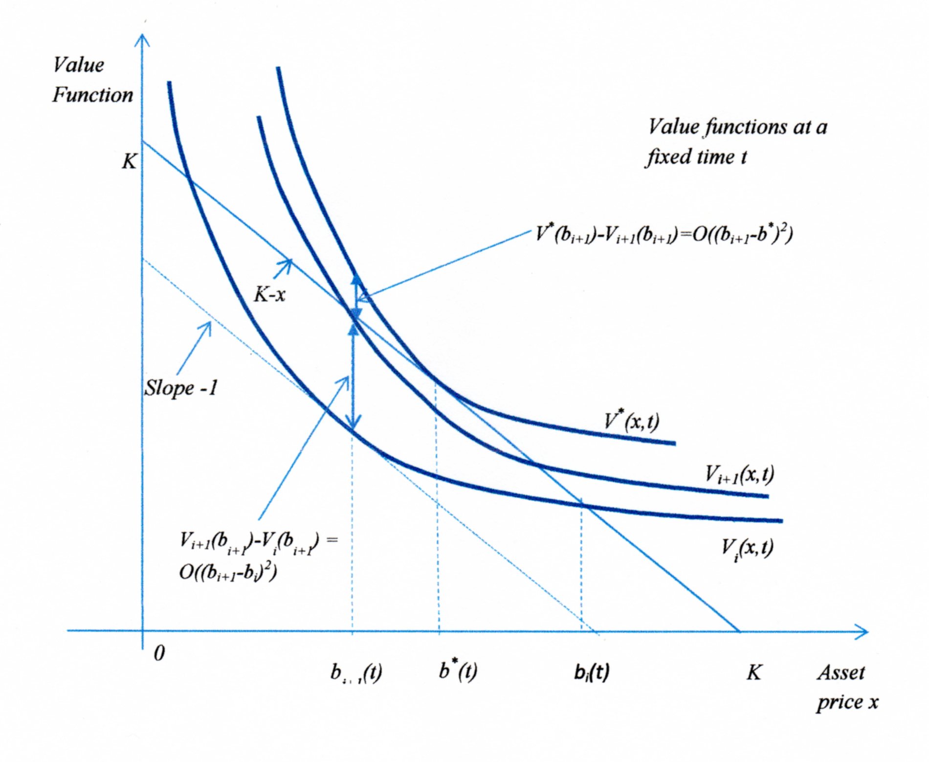
The solution of the Black–Scholes problem $V^{*}$ with boundary condition $V^{*}(b^{*}(t),t)=K-b^{*}(t)$ satisfies the smooth pasting $\frac{\partial{V^{*}(b^{*}(t),t)}}{\partial{x}}=-1$ , and vanishes as $x$ tends to infinity. (See Figure 4.1). Let $b_{i}$ and $b_{i+1}$ be two successive boundaries, as specified by the PIA algorithm. Then, from the construction of $b_{i+1}$ , we apply $V_{i,x}(b_{i+1}(t),t)=-1$ . From the Taylor theorem for some $\hat{b}$ , we have that

V_{i}(b_{i}(t),t)=V_{i}(b_{i+1}(t),t)+V_{i,x}(b_{i+1}(t),t)(b_{i}(t)-b_{i+1}(t))+\frac{1}{2}V_{i,xx}(\hat{b},t)(b_{i}(t)-b_{i+1}(t))^{2}.

Thus,

	$\displaystyle V_{i}(b_{i+1}(t),t)$	$\displaystyle=K-b_{i}(t)+(b_{i}(t)-b_{i+1}(t))-\frac{1}{2}V_{i,xx}(\hat{b},t)(b_{i}(t)-b_{i+1}(t))^{2}$
		$\displaystyle=K-b_{i+1}(t)-\frac{1}{2}V_{i,xx}(\hat{b},t)(b_{i}(t)-b_{i+1}(t))^{2},$

and finally

V_{i+1}(b_{i+1}(t),t)-V_{i}(b_{i+1}(t),t)=\frac{1}{2}V_{i,xx}(\hat{b},t)(b_{i}(t)-b_{i+1}(t))^{2}.

(4.8)

Furthermore, for some $\dot{b}$ , we have from Taylor’s theorem that

V^{*}(b_{i+1}(t),t)=V^{*}(b^{*}(t),t)+V^{*}_{x}(b^{*}(t),t)(b_{i+1}(t)-b^{*}(t))+\frac{1}{2}V^{*}_{xx}(\dot{b},t)(b_{i+1}(t)-b^{*}(t))^{2}.

Because $V_{x}^{*}(b^{*},t)=-1$ and $V^{*}(b^{*},t)=K-b^{*}$ from the previous equation, we take

V^{*}(b_{i+1}(t),t)-V_{i+1}(b_{i+1},t)=\frac{1}{2}V^{*}_{xx}(\dot{b},t)(b_{i+1}(t)-b^{*}(t))^{2}.

(4.9)

Applying Taylor’s theory to the partial $x$ derivatives, we have that for some $\bar{b}$

V^{*}_{x}(b_{i+1}(t),t)=V^{*}_{x}(b^{*}(t),t)+V_{xx}^{*}(\bar{b},t)(b_{i+1}(t)-b^{*}(t)).

Because $V^{*}_{x}(b^{*}(t),t)$ = $V_{i,x}(b_{i+1}(t),t)$ = $-1$ , subtracting the last equation from $V_{i+1}$ at $b_{i+1}$ , we have

	$\displaystyle V_{i+1,x}(b_{i+1}(t),t)$	$\displaystyle=V_{i+1,x}(b_{i+1}(t),t)-V^{*}_{x}(b_{i+1}(t),t)+V_{i,x}(b_{i+1}(t),t)$
		$\displaystyle+V_{xx}^{}(\bar{b},t)(b_{i+1}(t)-b^{}(t)),$

and so

	$\displaystyle V_{xx}^{}(\bar{b},t)(b_{i+1}(t)-b^{}(t))$	$\displaystyle=V_{i+1,x}(b_{i+1}(t),t)-V_{i,x}(b_{i+1}(t),t)$
		$\displaystyle+V^{*}_{x}(b_{i+1}(t),t)-V_{i+1,x}(b_{i+1}(t),t).$

Taking absolute values

	$\displaystyle\left\|V_{xx}^{}(\bar{b},t)(b_{i+1}(t)-b^{}(t))\right\|$	$\displaystyle\leq\left\|V_{i+1,x}(b_{i+1}(t),t)-V_{i,x}(b_{i+1}(t),t)\right\|$
		$\displaystyle+\left\|V_{i+1,x}(b_{i+1}(t),t)-V^{*}_{x}(b_{i+1}(t),t)\right\|.$

Equations (4.8) and (4.9) show that on the boundary $b_{i+1}$ , the functions $V_{i+1}$ and $V^{*}$ differ by an order of $[b_{i+1}(t)-b^{*}(t)]^{2}$ , whilst $V_{i}$ and $V_{i+1}$ differ by an order of $[b_{i+1}(t)-b_{i}(t)]^{2}$ . Note (see [18]) that at $b^{*}$ the second derivative of the optimal value function equals $V^{*}_{xx}(b^{*}(t),t)=\frac{2rK}{\sigma^{2}b^{*2}}$ and is therefore bounded in the vicinity of $b^{*}$ for the interval $[0,T]$ . Thus, for sufficiently small differences in the boundaries, and by virtue of AP (4.7), there exist constants $\alpha$ , $c_{1}$ , and $c_{2}$ such that

\alpha\lvert b_{i+1}(t)-b^{*}(t)\rvert\leq c_{1}(b_{i+1}(t)-b_{i}(t))^{2}+c_{2}(b_{i+1}(t)-b^{*}(t))^{2}.

(4.10)

By writing $\left(b_{i+1}(t)-b_{i}(t)\right)^{2}$ as $\left(b_{i+1}(t)-b^{*}(t)+b^{*}(t)-b_{i}(t)\right)^{2}$ and expanding the previous inequality, Equation (4.10) becomes

\alpha\lvert b_{i+1}(t)-b^{*}(t)\rvert-(c_{1}+c_{2})(b_{i+1}(t)-b^{*}(t))^{2}+2c_{1}(b_{i+1}(t)-b^{*}(t))(b_{i}(t)-b^{*}(t))\leq c_{1}(b_{i}(t)-b^{*}(t))^{2}.

Because $|b_{i+1}(t)-b^{*}(t)|$ and $|b_{i}(t)-b^{*}(t)|$ are sufficiently small, the above inequality becomes

\alpha\lvert b_{i+1}(t)-b^{*}(t)\rvert\leq c_{1}(b_{i}(t)-b^{*}(t))^{2}.

(4.11)

Supposing that $\alpha$ , $c_{1}$ , and $c_{2}$ are bounded away from $0$ and $\infty$ , the above inequality can be written as

\left\|b_{i+1}(t)-b^{*}(t)\right\|_{\infty}\leq c\left\|b_{i}(t)-b^{*}(t)\right\|^{2}_{\infty},

(4.12)

where $c=\frac{c_{1}}{\alpha}$ .

As stated earlier, the application of AP in the previous proof is justified if the values $V_{i}(x,t)$ generated are eventually of the form $V_{i}(x,t)=V^{*}(x,t)+\lambda_{i}h(x,t)$ for some function $h$ . The constants involved in the AP depend on the boundary $b_{i}$ but are independent of $i$ when the boundaries are close to $b^{*}$ . The computations reported in Section 4.6 corroborate the applicability of this assumption.

4.5 A Policy Iteration Algorithm for Free Boundary Stochastic Control Problems

The policy improvement used in the previous section relied on examining the extension of the value function inside the stopping region, which makes sense if we want to assess delaying the exercise. The same principle can be applied to general free boundary control problems and such a procedure is presented here, first for deterministic systems and then for stochastic ones. Several simplifying assumptions are made and only a monotonicity result is given while value or policy convergence is not examined.

Consider the control problem to determine

\sup_{u,T}\int_{t_{0}}^{T}f(x,\tau,u)d\tau+F(x_{T},T),

with $x\in\mathbb{R}^{n}$ satisfying the DE

\frac{dx}{dt}=g(x,t,u)\;\;\;x(t_{0})=x_{0}.

(4.13)

The end point $T$ is freely chosen. It is assumed that $u=u(x,t)$ is an acceptable control in that the resulting differential equation (4.13) has a solution.

A stopping policy $\pi^{k}=\left\{u_{k}(x,t),\Delta^{k}_{t}\right\}$ consists of an acceptable control $u_{k}$ and a collection of stopping regions $\Delta^{k}_{t}\subset\mathbb{R}^{n}$ for $t\geq t_{0}$ as well as continuation regions $C^{k}_{t}=\mathbb{R}^{n}-\Delta^{k}_{t}$ . Applying $\pi^{k}$ for a $x_{0}$ in the continuation region for $t_{0}$ consists of using the specified control to obtain a trajectory $x^{k}_{t}$ and stopping when it first enters a stopping region, i.e. at $T^{k}=\min_{t}\left\{t\geq t_{0}\;|\;x^{k}_{t}\in\Delta^{k}_{t}\right\}$ , assuming $T^{k}$ to be finite. The value of $\pi_{k},\;V^{k}(x,t)$ , is defined in the continuation region as

V^{k}(x_{0},t_{0})=\int_{t_{0}}^{T^{k}}f(x^{k},\tau,u^{k})d\tau+F(x_{T^{k}},T^{k}).

(4.14)

For a $x_{0}$ in the stopping region of $t_{0}$ the value is by definition $F(x_{0},t_{0})$ and thus the value $U^{k}(x,t)$ achieved by the stopping policy $\pi^{k}$ is

U^{k}(x,t)=\left\{\begin{array}[]{lrr}V^{k}(x,t),&x\in C^{k}_{t},&Continuation\;Region,\\ F(x,t),&x\in\Delta^{k}_{t},&Stopping\;Region.\end{array}\right.

To extend the continuation value $V^{k}$ in the stopping region we assume that for $(x_{0},t_{0})$ in the stopping region there is a prior time $T^{k}$ and a corresponding state $x_{T^{k}}$ on the boundary of $\Delta^{k}_{T^{k}}$ such that the process moves using the specidied control from $x_{T^{k}}$ to $x_{0}$ at time $t_{0}>T^{k}$ while staying inside the stopping region. The $V^{k}$ is again given by (4.14).

A new policy $\pi^{k+1}=\left\{u_{k+1}(x,t),\Delta^{k+1}_{t}\right\}$ is an improvement provided it is both a control and a stopping region improvement, namely the following conditions hold:

a)

Control improvement.

\!\!\!\!\!\!f(x,t,u^{k+1})+g(x,t,u^{k+1})V^{k}_{x}(x,t)\geq f(x,t,u^{k})+g(x,t,u^{k})V^{k}_{x}(x,t)\;\;\forall x,t.

(4.15)

A greedy choice would be to select the control that maximizes the right hand side.

b)

Stopping region improvement. In the new termination region the immediate exercise value must be greater than the continuation using $\pi_{k}$ , namely

\Delta^{k+1}_{t}\subseteq\left\{x\mid F(x,t)\geq V^{k}(x,t)\right\}.

A greedy choice would be

\Delta^{k+1}_{t}=\left\{x\mid x=\arg\max_{x}[F(x,t)-V^{k}(x,t)]\right\}.

This particular choice makes stopping difficult and must be proven consistent with the previously stated requirement of finite stopping times $T^{k}<\infty$ .

c)

Termination. The algorithm stops if it is not possible to improve on either criterion, namely the control $u^{k}$ maximizes the Hamiltonian $f+gV^{k}_{x}$ and $F(x,t)\leq V^{k}(x,t)\;\forall x,t$ . Approximate termination criteria could involve $\|u_{k+1}-u_{k}\|$ and/or $\|V^{k+1}-V^{k}\|$ .

The value of the updated policy $V^{k+1}$ is an improvement, i.e. $V^{k+1}(x,t)\geq V^{k}(x,t)$ for all $(x,t)$ . To show this, it is noted that for acceptable $u^{k+1},u^{k}$ the functions $V^{k+1},V^{k}$ satisfy the value PDE’s:

f(x,t,u^{l})+g(x,t,u^{l})V^{l}_{x}(x,t)+V^{l}_{t}(x,t)=0\quad l=k,k+1.

(4.16)

Given the choice of $u^{k+1}$ we have the following relations:

\begin{split}f(x,t,u^{k+1})+&g(x,t,u^{k+1})V^{k}_{x}(x,t)+V^{k}_{t}(x,t)\geq\\ &f(x,t,u^{k})+g(x,t,u^{k})V^{k}_{x}(x,t)+V^{k}_{t}(x,t)=0\end{split}

(4.17)

Substituting $f$ from (4.16) with $l=k+1,$ we have

\left[V^{k}_{t}(x,t)-V^{k+1}_{t}(x,t)\right]+g(x,t,u^{k+1})\left[V^{k}_{x}(x,t)-V^{k+1}_{x}(x,t)\right]\geq 0.

(4.18)

Applying the control $u^{k+1}$ starting at $(t_{0},x_{0})$ in the continuation region, we obtain a trajectory $x^{k+1}$ on which the difference $\left[V^{k}_{t}(x,t^{k+1})-V^{k+1}_{t}(x,t^{k+1})\right]$ equals the left hand side of (4.18). Recalling the assumption that the termination time $T^{k+1}$ is finite and integrating (4.18) on $x^{k+1}$ from $t_{0}$ to $T^{k+1}$ we obtain

V^{k}(x^{k+1}_{T^{k+1}},T^{k+1})-V^{k+1}(x^{k+1}_{T^{k+1}},T^{k+1})-V^{k}(x_{0},t_{0})+V^{k+1}(x_{0},t_{0})\geq 0.

(4.19)

By the choice of $T^{k+1}$ the difference of the first two terms is non-positive and thus $V^{k+1}(x_{0},t_{0})\geq V^{k}(x_{0},t_{0})$ . To show the inequality for an initial point $(x_{0},t_{0})$ inside the stopping region the calculation can be repeated starting from the prior point $(x^{k+1}_{T^{k+1}},T^{k+1})$ from which the control $u^{k+1}$ drives the system to $(t_{0},x_{0})$ .

As in Theorem 4.2 ii), we can choose the stopping region improvement such that the value of the stopping policies is everywhere nondecreasing i.e. $U^{k+1}(x,t)\geq U^{k}(x,t)$ . This can be done if the stopping region modifications $\left[\Delta^{k+1}_{t}-\Delta^{k}_{t}\right]\cup\left[\Delta^{k}_{t}-\Delta^{k+1}_{t}\right]$ are a subset of the connected region in which $V^{k}\leq F$ and includes the boundary of $\Delta^{k}_{t}$ , and then, if necessary, perform the second modification in Theorem 4.2 ii.

The stochastic control case is similar, but the assumptions required are stricter. Consider a stochastic control system

dx=g(x,t,u)dt+\sigma(x,t,u)dz\;\;\;x(t_{0})=x_{0}.

(4.20)

We want to determine

\sup_{u,T}E\left[\int_{t_{o}}^{T}f(x,\tau,u)d\tau+F(x_{T},T)\right].

(4.21)

We use the same definition of a policy $\pi^{k}=\left\{u_{k}(x,t),\Delta^{k}_{t}\right\}$ as in the deterministic case and consider the value function

V^{k}(x_{0},t_{0})=E\left[\int_{t_{0}}^{T^{k}}f(x^{k},\tau,u^{k})d\tau+F(x_{T^{k}},T^{k})\mid x(t_{0})=x_{0}\right].

(4.22)

Starting outside the termination region the stopping time is given by

T^{k}=\min_{t}\left\{t\geq t_{0}\mid x^{k}_{t}\in\Delta^{k}_{t}\right\}.

On the other hand if $(x_{0},t_{0})$ is inside the termination region, we consider the set of points $(x_{T^{k}},T^{k})$ on the termination region boundaries from which the specified control leads $x^{k}$ to $(x_{0},t_{0})$ while staying inside the termination region. Expectation is taken over the set consisting of these points $(x_{T^{k}},T^{k})$ conditional on the process reaching $(x_{0},t_{0})$ .

As in the deterministic case a policy $\pi_{k+1}=\left\{u_{k+1}(x,t),\Delta^{k+1}_{t}\right\}$ is an improvement provided it is both a control and a stopping region improvement, namely:

a)

Control improvement.

	$\displaystyle f(x,t,u^{k+1})+g(x,t,u^{k+1})V^{k}_{x}(x,t)+\frac{1}{2}\sigma^{2}(x,t,u^{k+1})V^{k}_{xx}(x,t)$	$\displaystyle\geq$
	$\displaystyle f(x,t,u^{k})+g(x,t,u^{k})V^{k}_{x}(x,t)+\frac{1}{2}\sigma^{2}(x,t,u^{k})V^{k}_{xx}(x,t).$			(4.23)

b)

Stopping region improvement. The immediate termination value must be greater than the continuation using $\pi_{k}$ , namely

\Delta^{k+1}_{t}\subseteq\left\{x\mid F(x,t)\geq V^{k}(x,t)\right\}.

If $\||F-V^{k}\|_{\infty}=M,$ then one could select as stopping region the $x$ ’s for which the difference $F-V^{k}$ is greater than $M-\epsilon$ . A greedy choice would be

\Delta^{k+1}_{t}=\left\{x\mid x=\arg\max_{x}[F(x,t)\geq V^{k}(x,t)]\right\}.

This choice would make stopping difficult and must be shown consistent with the requirement of finite expected stopping times $E(T^{k})<\infty$ which later in this section will be shown necessary for the algorithm to be improving.

c)

Termination: As in the deterministic system.

We assume that the controls $u^{k}$ lead to strong solutions of the stochastic system, a complication dealt in detail in [26]. Then, the values $V^{k+1},V^{k}$ corresponding to the policies $\pi_{k+1},\pi_{k},$ satisfy the PDE’s

	$\displaystyle f(x,t,u^{k})+g(x,t,u^{k})V^{k}_{x}(x,t)+\frac{1}{2}\sigma^{2}(x,t,u^{k})V^{l}_{xx}(x,t)+V^{k}_{t}(x,t)=0,$		(4.24)
	$\displaystyle f(x,t,u^{k+1})+g(x,t,u^{k+1})V^{k+1}_{x}(x,t)+\frac{1}{2}\sigma^{2}(x,t,u^{k+1})V^{l}_{xx}(x,t)+V^{k+1}_{t}(x,t)=0.$		(4.25)

The conditions for the boundary of the corresponding stopping region for the above equations are $F(x,t)=V^{k}(x,t)$ and $F(x,t)=V^{k+1}(x,t)$ respectively. We assume there exist such solutions. From the control boundary (4.18) applies that,

		$\displaystyle f(x,t,u^{k+1})+g(x,t,u^{k+1})V^{k}_{x}(x,t)+\frac{1}{2}\sigma^{2}(x,t,u^{k+1})V^{k}_{xx}(x,t)+V^{k}_{t}(x,t)\geq$
		$\displaystyle f(x,t,u^{k})+g(x,t,u^{k})V^{k}_{x}(x,t)+\frac{1}{2}\sigma^{2}(x,t,u^{k})V^{k}_{xx}(x,t)+V^{k}_{t}(x,t)=0.$

If we replace the term $f(x,t,u^{k+1})$ according to (4.25) in the left of the above inequality we have

	$\displaystyle\left[V^{k}_{t}(x,t)-V^{k+1}_{t}(x,t)\right]+g(x,t,u^{k+1})\left[V^{k}_{x}(x,t)-V^{k+1}_{x}(x,t)\right]$	$\displaystyle+$
	$\displaystyle\sigma^{2}(x,t,u^{k+1})/2\left[V^{k}_{xx}(x,t)-V^{k+1}_{xx}(x,t)\right]$	$\displaystyle\geq 0.$		(4.26)

If $x^{k+1}$ is the solution of the stochastic system (4.20), when the control is $u^{k+1}$ , we then consider the difference to the successive values $W^{k}(x^{k+1},t)=V^{k}(x^{k+1},t)-V^{k+1}(x^{k+1},t)$ . Then, from Ito’s Lemma and assuming a strong solution for the differential equation

dW^{k}=(W^{k}_{t}+gW^{k}_{x}+\frac{\sigma^{2}}{2}W^{k}_{xx})dt+\sigma W^{k}_{x}dz.

(4.27)

By virtue of (4.26), the coefficient appearing in $dt$ is nonnegative. Therefore, integrating (4.27) from $t_{0}$ to $T^{k+1}$ we obtain the inequality

W^{k}(x_{T^{k+1}},T^{k+1})-W^{k}(x_{0},t_{0})\geq\int_{t_{0}}^{T^{k+1}}\sigma W^{k}_{x}dz.

(4.28)

Again by the construction of the stopping time $T^{k+1},$ the first term is non positive. Furthermore, taking expectations and assuming $E(T^{k+1})<\infty$ we have by Dynkin’s lemma [77] that the expectation of the right hand integral vanishes. Consequently, $W^{k}(x_{0},t_{0})\leq 0$ leading to the desired inequality

V^{k+1}(x_{0},t_{0})\geq V^{k}(x_{0},t_{0}),

everywhere, inside or outside the stopping region. As in the deterministic case we can choose the modifications so that the stopping policy values $U^{k}$ are everywhere nondecreasing.

We collect the assumptions made in the exposition of the PIA for the free boundary stochastic system:

a): The controls $u^{k}$ lead to strong solutions.
b): The PDE’s (4.16) with boundary values at the stopping region boundaries have smooth solutions allowing the use of Ito’s Lemma.
c): The corresponding stopping times have finite expectations.

Subject to all these assumptions the PIA leads to monotonically improving policies. In its application to the American Put problem the control improvement is superfluous, since it is only the end point value that determines the payoff. Note also that the algorithm provides yet another proof of the necessity of smooth pasting.

4.6 Implementation, Accuracy and Computational Results

The crucial step in the implementation of the proposed algorithm is the solution of Equation (4.5) for a given boundary specified at discrete points, but not necessarily coinciding with the standard, uniform discretisation. In order to solve the equation above the boundary the popular implicit Euler method is used (see for example [23], [7]), modified in the vicinity of the boundary where the derivative estimates are adjusted to take into account the grid non uniformity. A piecewise linear boundary is implemented although a smooth interpolation would have been more accurate; however this simple approach suffices for the fine discretisation used. As in [7] the derivatives of the value function (and not the function itself) are set to zero at a large asset price and verified that increasing it does not affect the results. Using standard arguments as in [24], the error in the value function is $O(\Delta t+\Delta x^{2})$ in the region above the boundary. The reason that the Crank-Nicolson method wasn’t used is twofold: the Crank Nicolson method is unconditional stable in $l_{2}$ norm. This, together with consistency, ensures convergence in the $l_{2}$ norm for initial data which lies also in $l_{2}$ . Moreover the order of convergence may be less than the second order achieved for smooth initial data, see for example [29]. Even though there are modifications of Crank-Nicolson method like the Rannacher one [57] that retain the second order accuracy also for $l_{2}$ smooth initial data, they would require a more complicated adjustment near the boundary. Our simpler implementation is sufficient to clarify the algorithm’s features. In the single asset case these refinements were not necessary for a successful implementation but may prove crucial in a multidimensional treatment.

The algorithm requires the solution of (4.5) below as well as above the boundary. As stated earlier, extending the solution smoothly below the boundary is an initial value problem, whose error estimate increases exponentially and the implementations that tried to extend the solution below the boundary diverged fast. In the cases where the boundary had to be decreased the local updating that was used in Equation (4.29) proved to be satisfactory.

The computations show that the algorithm converges at a boundary $\tilde{b}$ on which the asset derivative equals $-1$ to several decimals. Consequently, the boundary error $\parallel\tilde{b}-b^{*}\parallel_{\infty}$ is of order $O(\Delta x)$ provided that the discretisation satisfies $\Delta t\leq\Delta x^{2}$ . To show this, note that the partial derivative estimate under this condition is accurate to $O(\Delta x)$ . Moreover, let $V,b$ be the current value and boundary, and $V^{*},b^{*}$ the corresponding optimal ones. Then, by the arguments in Section 4.4, we have

	$\displaystyle V(b(t),t)-V^{*}(b(t),t)$	$\displaystyle=V^{}_{xx}(b^{},t)(b-b^{*})^{2}+O(\Delta b)^{3},$
	$\displaystyle V^{*}_{x}(b,t)$	$\displaystyle=-1+V^{}_{xx}(b^{},t)(b-b^{*})+O(\Delta b)^{2},$

and $V_{x}(b,t)=-1+O(\Delta x)$ . By AP (4.7) applied on the boundary b and noting that $V,V^{*}$ differ by a quadratic term, so will their derivatives, and thus

V^{*}_{x}(b,t)=-1+V^{*}_{xx}(b^{*},t)(b-b^{*})+O(\Delta b)^{2}=V_{x}(b,t)=-1+O(\Delta x).

Consequently, $\|b-b^{*}\|_{\infty}=O(\Delta x)$ . It is mentioned that for a Crank-Nicolson type scheme and smooth enough initial data a discretisation of $\Delta x=\Delta t$ would have sufficed for an $O(\Delta x)$ derivative error, and the computational burden would have improved by an order of magnitude.

The boundary updating stipulated by the algorithm is implemented in a simplified fashion as follows: At the $k$ -th iteration with a boundary $b_{k}$ we calculate the value $V^{k}(x,t)$ for $x\geq b_{k}(t)$ . We then compute $\max\{[K-x]^{+}-V^{k}(x,t)\}$ and if it is positive we set the new boundary $b_{k+1}(t)$ at the value attaining the maximum. If it occurs at an $x$ below the boundary is updated by maximizing the local quadratic approximation and obtain the updating formula

b_{k+1}(t)=b_{k}(t)-(1+V^{k}_{x})/V^{k}_{xx}.

(4.29)

The derivatives $V^{k}_{x},V^{k}_{xx}$ are to be evaluated at the boundary and standard one sided formulas were applied. This simplified updating did not affect the claimed speed of convergence since these refer only to the vicinity of the optimal boundary where the approximate updating is accurate. It is noted that the second derivative expression has the same accuracy as the first derivative one since it depends on it through Equation (4.5).

The implementation displayed the value monotonicity property claimed, and all values generated on the $x,t$ grid were monotonically increasing for the chosen discretisation. This property would probably not hold for a coarser discretisation, and would be of interest to prove for the corresponding methods, as in [14], the necessary conditions under which the monotonicity holds.

The algorithm is applied to a recent example appearing in Zhu et. al. [79] that uses a novel integral equation for the boundary. The example has a risk free interest rate $r=10\%$ , volatility $\sigma=30\%$ , exercise price $K=100$ and horizon $T=1$ . We applied the PIA algorithm with $\Delta x=0.05\;\;\Delta t=0.0025$ and the computations are in agreement with those in [79] as shown in Table 4.1. A linear interpolation was used to obtain Zhu’s times to expiry. We also extended the horizon calculation to $T=10$ units with $\Delta x=0.1$ , and we obtained an exercise boundary of 69.2371, slightly above the perpetual put value 68.9655, obtained from the expression [28] $K_{exer}\frac{\phi}{1-\phi},$ with $\phi=\sigma^{-2}\left(\sigma^{2}/2-r-\sqrt{(r-\sigma^{2}/2)^{2}+2r\sigma^{2}}\right).$

Table 4.1: Computational Results

Time	PIA	Zhu	Adjusted
to Expiry		(average)	Brennan Schwartz
0.0868	87.3735	87.3548	87.3842
0.1515	85.0142	84.9176	85.0140
0.2321	83.0725	82.9635	83.0649
0.3039	81.8029	81.7002	81.7972
0.3697	80.8666	80.7677	80.8589
0.4480	79.9438	79.8531	79.9364
0.5083	79.3373	79.2523	79.3312
0.5761	78.7375	78.6575	78.7328
0.6521	78.1472	78.0710	78.1428
0.7376	77.5655	77.4928	77.5623
0.8335	76.9949	76.9246	76.9919
0.9413	76.4356	76.3635	76.4336

The computational cost per boundary calculation is $O(mn),$ with $m,n$ being the number of grid points in time and asset price, respectively. Since $\Delta x^{2}=\Delta t$ the aforementioned cost is $O(n^{3})$ flops. The number of iterations required to achieve smooth pasting i.e. the derivative estimate being -1 to several significant figures, was of the order of 10. However, if we stop when the derivative is $O(\Delta x^{2})$ close to -1, we have reached the expected error level and might as well stop. This is achieved in about 5 iterations even when starting from an inaccurate initial policy.

The claimed quadratic convergence of the algorithm was analyzed in the above computations. We examine whether the error $e_{n}=\|b_{n}(t)-b^{*}(t)\|_{\infty}$ satisfies $e_{n}\leq\alpha e^{2}_{n-1}$ or in logarithmic terms $\eta_{n}=a+2\eta_{n-1}$ with $\eta_{n}=ln(e_{n})\quad a=ln(\alpha)$ . We estimated $e_{n}$ by sampling over equidistant $t_{i}$ ’s, and present the results in Figures 4.2, 4.3, and 4.4. We expect the quadratic relation to hold whenever the errors are sufficiently small, but not smaller than $O(\Delta x)$ . Specifically, Figure 4.2 shows that the errors satisfying these conditions are those in iterations 6-10. The results of these iterations are shown in Figures 4.3 and 4.4. In Figure 4.3 we present the logarithmic error behavior and note the expected concave shape resulting from the solution of the difference equation $\eta_{n}=2^{n}(\eta_{0}+a)-a$ , the coefficient $\eta_{o}+a$ of the power term assumed negative, a reasonable assumption. In Figure 4.4 we observe that the plot of $\eta_{n}$ vs $\eta_{n-1}$ has a slope close to 2 for the above iterations. For smaller error values we see in Figure 4.2 that they decrease linearly and not quadratically, but this is of little interest since the convergence to the boundary is only $O(\Delta x)$ accurate.

In Figure 4.5 we illustrate the generated boundary sequence. Starting with an initial boundary far from the optimal, the algorithm generates wildly fluctuating ones for a few iterations, and then settles on the limiting one. This behavior is not inconsistent with the monotonicity property which refers to the values and not the boundaries generated.

A fast method like Brennan and Schwartz [7], can be easily modified by the Policy Iteration principle to produce more accurate results. Let the value obtained by that method at $x_{j},t_{i}$ be $\tilde{V}(x_{j},t_{i})$ . A point $x_{j}$ is considered as a boundary one if $K-x_{j}\leq\tilde{V}(x_{j},t_{i})$ but at the immediately lower point $x_{j-1}$ the opposite holds. It is clear that the derivative at these points is greater than $-1$ , and hence the actual boundary should be at a lower point. Having solved (4.5) above the boundary just once the local update (4.29) is then applied. These calculations are presented in the last column of Table 4.1; the method was applied with $\Delta x=0.05,\;\Delta t=\Delta x^{2}$ and the results are in close agreement with those obtained by the other methods. The non adjusted Brennan and Schwartz boundaries differ by about $1\%$ for $\Delta x=0.05$ . Finally, for a horizon of $T=10$ the boundary is at 70.04, relatively close to the perpetual put value 68.97.

The above computational results are further verified by a simple simulation. The asset process $z_{t}$ was generated by the exponential formula $z_{t+\delta t}=z_{t}\exp\left((r-\frac{\sigma^{2}}{2})\delta t+\sigma\epsilon_{t}\sqrt{\delta t}\right)$ with $\epsilon_{t}$ independent samples from a standard normal distribution. The time step $\delta t$ used was much smaller than the boundary discretisation $\Delta t$ , since a crossing of the linearized boundary by $z_{t}$ is sufficient but not necessary for a crossing by the asset process. Thus, it is expected the value obtained in the simulation to be smaller than the one calculated by PIA. This is indeed observed, see Table 4.2.

Table 4.2: Simulation Results

Time to Expiry = 0.5
Asset Price	Option	Simulation	Standard
	Value	result	Deviation
86.56	15.236	14.860	0.215
96.94	9.558	9.422	0.214
107.32	5.883	5.965	0.184
117.71	3.563	3.510	0.149
128.09	2.142	2.216	0.119
138.47	1.271	1.280	0.091
148.85	0.751	0.487	0.055
159.24	0.445	0.321	0.043
169.62	0.267	0.223	0.035
180.00	0.168	0.146	0.030

Conclusions

In this thesis, the numerical solution of three different classes of problems have been studied. Specifically, we have proposed new techniques and their theoretical analysis has been performed, accompanied by a wide set of numerical experiments, for investigating further the effectiveness and performance of our approach. The first two belong to the research area of numerical linear algebra and concern the spectral analysis and preconditioning of the coefficient matrix of large structured linear systems. The third concerns a problem from economics namely the pricing of an American put option.

In the first set of problems the singular value distribution of the matrix sequence $\{h(T_{n}(f))\}_{n}$ and the eigenvalue distribution of the symmetrised matrix sequence $\{Y_{n}h(T_{n}(f))\}_{n}$ was provided. The spectral assymptotic behavior of this matrix sequences was studied under the assumption that $h$ is an analytic function at 0, with radious of convergance $r$ , and $f\in L^{\infty}([-\pi,\pi])$ with $\|f\|_{\infty}<r$ so that $h\circ f\in L^{\infty}([-\pi,\pi])\subset L^{1}([-\pi,\pi])$ . Taking advantage of this analysis circulant preconditioners were proposed, and the eigenvalue distribution of the preconditioned matrix sequences was given. All theoretical results were numerically confirmed. A desirable future development in this class of problems is the investigation on the possibility of relaxation of the given conditions:

A): If the function $h$ is analytic in a given disk centered at $z_{0}\neq 0$ , then the arguments working in the case $z_{0}=0$ can be repeated verbatim also in the new setting.
B): When $f\in L^{1}([-\pi,\pi])$ (but $f$ does not belong to $L^{\infty}([-\pi,\pi])$ ), then the situation is more complicated and a further step of analysis is required. It could be used the cut–off argument as in [78, 74] and the versatility of the a.c.s. notion. An alternative to the cut-off idea is the use of polynomials such as the Cesaro sum $f$ converging to $f$ in the $L^{1}([-\pi,\pi])$ metric plus the trace-norm estimates of $T_{n}(f)$ derived in [69].

The second problem that we studied concerned the theoretical and numerical exploration of proper preconditioners based on the spectral symbols of the coefficient matrix for FDE problems. Beside the theoretical study, a comparison between the new and old preconditioners was conducted, especially those presented in [9, 42]. As expected and numerically shown in Example 1 which concerned the one dimensional case, the proposed preconditioners performed slightly worse, at least in a sequential model of computation, than the tridiagonal preconditions proposed in [9], because of the computational complexity. However, in the two dimensional case as discussed in Examples 2 and 3, the proposed preconditioners did indeed perform better than the previously proposed multigrid-based or band preconditioners proposed and studied in [42]. Future directions of research may include more complex problems, further analysis, and more extensive numerical experimentation. Also, problems where the fractional derivatives are greater than 2 may be considered, since then it is expected the symbol-based preconditioners to be even more advantageous, maybe even in the one dimensional case.

For the pricing of an American put option an iterative algorithm was used. Taking advantage of the already known characteristics of the optimal value function it was shown theoretically and confirmed numerically that the proposed algorithm obtains monotonically increasing value functions and converges to the optimal one. Issues regarding the efficiency in multiple asset cases or how can the method be applied in a finite element context are to be concerned in future works.

In the same spirit of the iterative algorithm used here for pricing the American put option, we are working on a further work on the solution of Stefan problem. It consists of a boundary value problem which describes the evolution of the boundary between two faces–that is currently being developed. A preprint of this work is available [37].

Bibliography

[1] F. Avram. On bilinear forms in Gaussian random variables and Toeplitz matrices. Probab. Theory Related Fields, 79(1):37–45, 1988.
[2] O. Axelsson and G. Lindskog. On the rate of convergence of the preconditioned conjugate gradient method. Numer. Math., 48(5):499–523, 1986.
[3] N. Barakitis, S.-E. Ekström, and P. Vassalos. Preconditioners for fractional diffusion equations based on the spectral symbol. Numer. Linear Algebra Appl., (accepted).
[4] G. Barles, J. Burdeau, K. Romano, and N. Samsoen. Critical stock price near expiration. Appl. Math. Finance, 5:77–95, 1995.
[5] R. Bellman. Dynamic Programming. Princeton University Press, 1957.
[6] M. Benzi. Preconditioning techniques for large linear systems: A survey. J. Comput. Phys., 182(2):418–477, 2002.
[7] M. Brennan and E. Schwartz. The valuation of American put options. J. Finance, 32:449–462, 1977.
[8] P. Carr, R. Jarrow, and R. Myneni. Alternative characterizations of american put options. Math. Financ., 2:87–106, 1992.
[9] M. Donatelli, M. Mazza, and S. Serra-Capizzano. Spectral analysis and structure preserving preconditioners for fractional diffusion equations. J. Comput. Phys., 307:262–279, 2016.
[10] C. Estatico and S. Serra-Capizzano. Superoptimal approximation for unbounded symbols. Linear Algebra Appl., 428(2-3):564–585, 2008.
[11] D. Fasino and P. Tilli. Spectral clustering properties of block multilevel Hankel matrices. Linear Algebra Appl., 306(1-3):155–163, 2000.
[12] P. Ferrari, N. Barakitis, and S. Serra-Capizzano. Asymptotic spectra of large matrices coming from the symmetrization of Toeplitz structure functions and applications to preconditioning. Numer. Linear Algebra Appl., 28(1), 2020.
[13] P. Ferrari, I. Furci, S. Hon, M. A. Mursaleen, and S. Serra-Capizzano. The eigenvalue distribution of special 2-by-2 block matrix-sequences with applications to the case of symmetrized Toeplitz structures. SIAM J. Matrix Anal. Appl., 40(3):1066–1086, 2019.
[14] P. A. Forsyth and G. Labahn. Numerical methods for controlled hamilton-jacobi bellman pdes in finance. J. Comput. Finance, 11:1–44, 2007.
[15] C. Garoni and S. Serra-Capizzano. Generalized locally Toeplitz sequences: theory and applications. Vol. I. Springer, Cham, 2017.
[16] C. Garoni and S. Serra-Capizzano. Generalized locally Toeplitz sequences: theory and applications. Vol. II. Springer, Cham, 2018.
[17] C. Garoni, S. Serra-Capizzano, and P. Vassalos. A general tool for determining the asymptotic spectral distribution of Hermitian matrix-sequences. Operators and Matrices, 9:549–561, 2015.
[18] J. Goodman and D. Ostrov. On the early exercise boundary of the American put option. SIAM J. Appl. Math., 62:1823–1835, 2002.
[19] A. Greenbaum, V. Pták, and Z. Strakoš. Any nonincreasing convergence curve is possible for GMRES. SIAM J Matrix Anal. Appl., 17(3):465–469, 1996.
[20] U Grenander and G Szegő. Toeplitz forms and their applications. Chelsea Publishing Co., New York, second edition, 1984.
[21] S. Hon, M. A. Mursaleen, and S. Serra-Capizzano. A note on the spectral distribution of symmetrized Toeplitz sequences. Linear Algebra Appl., 579:32–50, 2019.
[22] S. Hon and A. Wathen. Circulant preconditioners for analytic functions of Toeplitz matrices. Numer. Algorithms, 79(4):1211–1230, 2018.
[23] J. Hull. Options, Futures and Other Derivatives. Pearson, 9th edition, 2017.
[24] E. Isaacson and H. Keller. Analysis of Numerical Methods. Dover, 1994.
[25] S. D. Jacka. Optimal stopping and the American put. Math. Financ., 1:1–14, 1991.
[26] S. D. Jacka and A. Mijatovic. On the policy improvement algorithm in continuous time. Stochastics, 89(1):348–359, 2017.
[27] I.J. Kim. The analytic valuation of american options. Rev. Financial Stud., 3:547–572, 1990.
[28] R. Kohn. Lecture notes in PDE’s for Finance, 2014.
[29] H. O. Kreiss, V. Thomée, and O. Widlund. Smoothing of initial data and rates of convergence for parabolic difference equations. Comm. Pure Appl. Math., 43:241–259, 1970.
[30] C. Lanczos. Solution of systems of linear equations by minimized iterations. J. Res. Natl. Bur. Stand., 49(1):33, 1952.
[31] S. T. Lee, X. Liu, and H. Sun. Fast exponential time integration scheme for option pricing with jumps. Numer. Linear Algebra Appl., 19(1):87–101, 2012.
[32] S. T. Lee, H. Pang, and H. Sun. Shift-invert Arnoldi approximation to the Toeplitz matrix exponential. SIAM J. Sci. Comput., 32(2):774–792, 2010.
[33] S. Lei and H. Sun. A circulant preconditioner for fractional diffusion equations. J. Comput. Phys., 242:715–725, 2013.
[34] J. Maeda and S. D. Jacka. Market driver volatility model via policy improvement algorithm. arXiv:1612.0078v1, 2016.
[35] E. Mageirou. Iterative techniques for Ricatti game equations. J. Optim. Theory Appl., 22:51–61, 1977.
[36] E. Magirou, P. Vassalos, and N. Barakitis. A policy iteration algorithm for the American put option and free boundary control problems. J. Comput. Appl. Math, 373:112544, 2020.
[37] E. Magirou, P. Vassalos, and N. Barakitis. On a boundary updating method for the scalar Stefan problem. arXiv preprint arXiv:2202.06418, 2022.
[38] M. Mazza and J. Pestana. Spectral properties of flipped Toeplitz matrices and related preconditioning. BIT, 59(2):463–482, 2019.
[39] H. McKean. A free boundary problem for the heat equation arising from a problem in mathematical economics. Ind. Manag. Rev., 6:32–39, 1965.
[40] M. Meerschaert and C. Tadjeran. Finite difference approximations for fractional advection–dispersion flow equations. J. Comput. Appl. Math., 172(1):65–77, 2004.
[41] M. Meerschaert and C. Tadjeran. Finite difference approximations for two-sided space-fractional partial differential equations. Appl. Numer. Math., 56(1):80–90, 2006.
[42] H. Moghaderi, M. Dehghan, M. Donatelli, and M. Mazza. Spectral analysis and multigrid preconditioners for two-dimensional space-fractional diffusion equations. J. Comput. Phys., 350:992–1011, 2017.
[43] D. Noutsos, S. Serra-Capizzano, and P. Vassalos. Spectral Equivalence and Matrix Algebra Preconditioners for Multilevel Toeplitz Systems: A Negative Result., pages 313–322. AMS, USA, 2001.
[44] D. Noutsos, S. Serra-Capizzano, and P. Vassalos. Matrix algebra preconditioners for multilevel Toeplitz systems do not insure optimal convergence rate. Theor. Comput. Sci, 315(2):557–579, 2004.
[45] D. Noutsos, S. Serra-Capizzano, and P. Vassalos. A preconditioning proposal for ill-conditioned Hermitian two-level Toeplitz systems. Numer. Linear Algebra Appl., 12(2-3):231–239, 2005.
[46] D. Noutsos, S. Serra-Capizzano, and P. Vassalos. Block band Toeplitz preconditioners derived from generating function approximations: analysis and applications. Numer. Math., 104(3):339–376, 2006.
[47] D. Noutsos, S. Serra-Capizzano, and P. Vassalos. The conditioning of FD matrix sequences coming from semi-elliptic differential equations. Linear Algebra Appl., 428(2-3):600–624, 2008.
[48] D. Noutsos, S. Serra-Capizzano, and P. Vassalos. Essential spectral equivalence via multiple step preconditioning and applications to ill conditioned Toeplitz matrices. Linear Algebra Appl., 491:276–291, 2016.
[49] D. Noutsos and P. Vassalos. New band Toeplitz preconditioners for ill-conditioned symmetric positive definite Toeplitz systems. SIMAX, 23(3):728–743, 2002.
[50] D. Noutsos and P. Vassalos. Superlinear convergence for PCG using band plus algebra preconditioners for Toeplitz systems. Comput. Math. with Appl., 56(5):1255 – 1270, 2008.
[51] C. C. Paige and M. A. Saunders. Solution of sparse indefinite systems of linear equations. SIAM J. Numer. Anal., 12(4):617–629, 1975.
[52] H. Pang and H. Hai-Wei Sun. Fast Numerical Contour Integral Method for Fractional Diffusion Equations. J. Sci. Comput., 66(1):41–66, 2015.
[53] H. Pang and H. Sun. Multigrid method for fractional diffusion equations. J. Comput. Phys., 231(2):693–703, 2012.
[54] S. V. Parter. On the distribution of the singular values of Toeplitz matrices. Linear Algebra Appl., 80:115–130, 1986.
[55] J. Pestana and A. Wathen. A preconditioned MINRES method for nonsymmetric Toeplitz matrices. SIAM J. Matrix Anal. Appl., 36(1):273–288, 2015.
[56] M. Puterman. Markov Decision Processes: Discrete Stochastic Dynamic Programming. John Wiley & Sons, Inc., New Jersey, 2005.
[57] R. Rannacher. Finite element solution of diffusion problems with irregular data. Numer. Math, 43:309–327, 1984.
[58] J. K. Reid. On the method of conjugate gradients for the solution of large sparse systems of linear equations. In Pro. the Oxford conference of institute of mathmatics and its applications, pages 231–254, 1971.
[59] B. Rynne and M. Martin Youngson. Linear Functional Analysis. Springer London, 2008.
[60] Y. Saad. Iterative Methods for Sparse Linear Systems. Society for Industrial and Applied Mathematics, 2003.
[61] Y. Saad and M. H. Schultz. GMRES: A generalized minimal residual algorithm for solving nonsymmetric linear systems. SIAM J. Sci. Comput., 7(3):856–869, 1986.
[62] T. Sauer. Numerical Analysis. Addison-Wesley Publishing Company, USA, 2nd edition, 2011.
[63] R. Scherer, S. L. Kalla, Y. Tang, and J. Huang. The Grünwald–Letnikov method for fractional differential equations. Comput. Math. with Appl., 62(3):902–917, 2011.
[64] S. Serra-Capizzano. A korovkin-type theory for finite Toeplitz operators via matrix algebras. Numerische Mathematik, 82(1):117–142, 1999.
[65] S. Serra-Capizzano. Korovkin tests, approximation, and ergodic theory. Mathematics of Computation, 69(232):1533–1559, 2000.
[66] S. Serra-Capizzano. Spectral behavior of matrix sequences and discretized boundary value problems. Linear Algebra Appl., 337:37–78, 2001.
[67] S. Serra-Capizzano. Generalized locally Toeplitz sequences: spectral analysis and applications to discretized partial differential equations. Linear Algebra Appl., 366:371–402, 2003.
[68] S. Serra-Capizzano. The GLT class as a generalized Fourier analysis and applications. Linear Algebra Appl., 419(1):180–233, 2006.
[69] S. Serra-Capizzano and P. Tilli. On unitarily invariant norms of matrix-valued linear positive operators. J. Inequal. Appl., 7(3):309–330, 2002.
[70] W.Y. Tian, H. Zhou, and W. Deng. A class of second order difference approximations for solving space fractional diffusion equations. Math. Comput., 84(294):1703–1727, 2015.
[71] P. Tilli. Locally Toeplitz sequences: spectral properties and applications. Linear Algebra Appl., 278(1-3):91–120, 1998.
[72] E. E. Tyrtyshnikov. New theorems on the distribution of eigenvalues and singular values of multilevel Toeplitz matrices. Dokl. Akad. Nauk, 333(3):300–303, 1993.
[73] E. E. Tyrtyshnikov. A unifying approach to some old and new theorems on distribution and clustering. Linear Algebra Appl., 232:1–43, 1996.
[74] E. E. Tyrtyshnikov and N. L. Zamarashkin. Spectra of multilevel Toeplitz matrices: advanced theory via simple matrix relationships. Linear Algebra Appl., 270:15–27, 1998.
[75] P. Vassalos. Asymptotic results on the condition number of FD matrices approximating semi-elliptic PDEs. Electron. J. Linear Algebra, 34:566–581, 2018.
[76] H. Wang, K. Wang, and T. Sircar. A direct $\mathcal{O}({N}\log^{2}{N})$ finite difference method for fractional diffusion equations. J. Comput. Phys., 229(21):8095–8104, 2010.
[77] D. Williams. Probability with martingales. Cambridge University Press, 1991.
[78] N. L. Zamarashkin and E. E. Tyrtyshnikov. Distribution of the eigenvalues and singular numbers of Toeplitz matrices under weakened requirements on the generating function. Mat. Sb., 188(8):83–92, 1997.
[79] S. P. Zhu, X. J. He, and X. P. Lu. A new integral equation formulation for American put options. Quant. Finance, 18:483–490, 2018.

		$\displaystyle\left\|\frac{1}{n}\sum_{j=1}^{n}F(\lambda_{j}(A_{n}))-F(\lambda_{j}(B_{n}))\right\|=$
		$\displaystyle\left\|\frac{1}{n}\sum_{j\notin N_{\epsilon}}F(\lambda_{j}(A_{n}))-F(\lambda_{j}(B_{n}))+\frac{1}{n}\sum_{j\in N_{\epsilon}}F(\lambda_{j}(A_{n}))-F(\lambda_{j}(B_{n}))\right\|\leq$
		$\displaystyle\left\|\frac{1}{n}\sum_{j\notin N_{\epsilon}}F(\lambda_{j}(A_{n}))-F(\lambda_{j}(B_{n}))\right\|+\left\|\frac{1}{n}\sum_{j\in N_{\epsilon}}F(\lambda_{j}(A_{n}))-F(\lambda_{j}(B_{n}))\right\|\leq$
		$\displaystyle\omega(\epsilon^{1/2};F)+\frac{1}{n}2\\|F\\|_{\infty}c\epsilon^{-1},$

	$\displaystyle\{\|c(T_{n}(h\circ f))\|\}_{n}\sim_{GLT,\sigma,\lambda}\|h\circ f\|,$	$\displaystyle\quad\{\|h(c(T_{n}(f)))\|\}_{n}\sim_{GLT,\sigma,\lambda}\|h\circ f\|,$		(2.11)
	$\displaystyle\{\|c(T_{n}(h\circ f))\|^{-1}\}_{n}\sim_{GLT,\sigma,\lambda}\|h\circ f\|^{-1},$	$\displaystyle\quad\{\|h(c(T_{n}(f)))\|^{-1}\}_{n}\sim_{GLT,\sigma,\lambda}\|h\circ f\|^{-1}.{}$		(2.12)

		$\displaystyle\{\|c(T_{n}(h\circ f))\|^{-1}h(T_{n}(h\circ f))\}_{n}=\{\|h(c(T_{n}(f)))\|^{-1}h(T_{n}(h\circ f))\}_{n}+\{\Delta_{n}\}_{n}\Rightarrow$
		$\displaystyle\{Y_{n}\|c(T_{n}(h\circ f))\|^{-1}h(T_{n}(h\circ f))\}_{n}=\{Y_{n}\|h(c(T_{n}(f)))\|^{-1}h(T_{n}(h\circ f))\}_{n}+\{Y_{n}\Delta_{n}\}_{n}\Rightarrow$
		$\displaystyle\{\|c(T_{n}(h\circ f))\|^{-1}Y_{n}h(T_{n}(h\circ f))\}_{n}=\{\|h(c(T_{n}(f)))\|^{-1}Y_{n}h(T_{n}(h\circ f))\}_{n}+\{Y_{n}\Delta_{n}\}_{n}$
		$\displaystyle=\{Q_{n}\}_{n}+\{Z_{n}\}_{n}+\{Y_{n}\Delta_{n}\}_{n}=\{Q_{n}\}_{n}+\{\hat{Z}_{n}\}_{n},$

Acknowledgment

Introduction

Part I Spectral Analysis and Preconditioned Iterative Solvers for Large Structured Linear Systems

Chapter 1 Generalized Locally Toeplitz Matrix Sequences

1.1 Singular Value, Eigenvalue Distribution, and Clustering of Matrix Sequences

Definition 1.1.

Remark 1.1.

Definition 1.2.

Theorem 1.1.

1.2 Approximation in Space of Matrix Sequences

Definition 1.3.

Theorem 1.2.

Proof.

Remark 1.2.

Proposition 1.2.1.

Proposition 1.2.2.

Theorem 1.3.

Proof.

Theorem 1.4.

Proof.

1.3 Approximating Classes of Sequences

Remark 1.3.

Definition 1.4.

Proposition 1.3.1.

Proposition 1.3.2.

Proof.

Theorem 1.5.

Theorem 1.6.

Proposition 1.3.3.

1.3.1 Zero Distributed Sequences

Definition 1.5.

Theorem 1.7.

Proof.

1.4 Circulant and Toeplitz Matrices

1.4.1 Toeplitz Matrices and Toeplitz Matrix Sequences

Definition 1.6.

Theorem 1.8.

Proof.

1.5 LT and GLT Matrix Sequences

1.5.1 LT Matrix Sequences

Definition 1.7.

Theorem 1.9.

1.5.2 GLT Matrix Sequences

Definition 1.8.

Chapter 2 Asymptotic spectra of large matrices coming from the symmetrisation of Toeplitz structure functions and applications to preconditioning

2.1 Eigenvalue Distribution of Symmetrised Toeplitz Matrix Sequences

Definition 2.1.

Theorem 2.1.

Proof.

2.2 Eigenvalue distribution of large matrices produced by the symmetrisation of Toeplitz structure functions

2.2.1 Matrix functions

Proposition 2.2.1.

2.2.2 Basic Results

Proposition 2.2.2.

Proof.

Theorem 2.2.

Proof.

2.3 Numerical Results

2.3.1 Spectrum of the {Yn​h​(Tn​(f))}n\{Y_{n}h(T_{n}(f))\}_{n}

Example 2.1.

Example 2.2.

Example 2.3.

Example 2.4.

2.3.2 Circulant Preconditioners for the Symmetrised Toeplitz Sequence

Definition 2.2.

Definition 2.3.

Remark 2.1.

Proposition 2.3.1.

Proposition 2.3.2.

Proof.

Proposition 2.3.3.

Proposition 2.3.4.

Proof.

Example 2.5.

Remark 2.2.

Example 2.6.

Example 2.7.

Chapter 3 Preconditioners for Fractional Diffusion Equations Based on the Spectral Symbol

3.1 Introduction

3.2 Definition of Fractional Derivative

2.3.1 Spectrum of the $\{Y_{n}h(T_{n}(f))\}_{n}$

Chapter 3 Preconditioners for Fractional Diffusion Equations
Based on the Spectral Symbol

3.6 The $\tau$ Preconditioners

3.6.1 The $\tau$ Preconditioner in one Dimension

Case I: $d_{\pm}$ are constants

Case II. $d_{-}(x)=d_{+}(x)>0$