Local Topology Inference of Mobile Robotic Networks under Formation Control
Abstract
The interaction topology is critical for efficient cooperation of mobile robotic networks (MRNs). We focus on the local topology inference problem of MRNs under formation control, where an inference robot with limited observation range can manoeuvre among the formation robots. This problem faces new challenges brought by the highly coupled influence of unobservable formation robots, inaccessible formation inputs, and unknown interaction range. The novel idea here is to advocate a range-shrink strategy to perfectly avoid the influence of unobservable robots while filtering the input. To that end, we develop consecutive algorithms to determine a feasible constant robot subset from the changing robot set within the observation range, and estimate the formation input and the interaction range. Then, an ordinary least squares based local topology estimator is designed with the previously inferred information. Resorting to the concentration measure, we prove the convergence rate and accuracy of the proposed estimator, taking the estimation errors of previous steps into account. Extensions on nonidentical observation slots and more complicated scenarios are also analyzed. Comprehensive simulation tests and method comparisons corroborate the theoretical findings.
I Introduction
Mobile robotic networks (MRNs) have received increasing attention in the last decades. Thanks to the mobility, flexibility, and distributed fashion, MRNs are widely deployed, e.g., surveillance, reconnaissance, search and environmental monitoring [2]. Among these applications, formation control serves as a fundamental technique to enhance the cooperation performance by maintaining a preset geometric shape [3]. Numerous methods have been proposed to obtain stable and robust formation control, see [4, 5] for a detailed review. Despite the large variety of the control methods, the interaction topology among robots is universal and critical for effective cooperation of MRNs. The topology characterizes the locality of information exchange, and determines the shape-forming stability and convergence.
Recent years have witnessed the emergence of many applications that necessitate advances in topology inference, which brings significant benefits in better understanding the system behaviors. Taking MRNs as the specific object, there are mainly two types of applications. First, from the security perspective, external attackers can utilize the topology inference method to find the critical robot that has significant control impacts in the formation, e.g., calculating the node degree and centrality [6], or identifying the leadership relationship in the formation [7]. With the topology information, more intelligent interception or herding tasks in military scenarios can be performed to control the formation [8, 9, 10, 11]. Second, from the perspective of performance improvement, inferring the topology of formation can support the self-configuration ability of MRNs [12]. For instance, when a robot disconnects with others, it can use the inferred local topology to keep coordination with the formation, by predicting the state and reconnecting with appropriate neighboring robots [13].
Mathematically, topology inference can be seen as a typical inverse modeling problem. Plenty of related works have been developed for various dynamic models [14, 15, 16, 17]. In relation to the basic consensus dynamics, the interaction topology is reconstructed by measuring the power spectral density of the network response to input noises, and node removal strategies are designed [18, 19]. For sparsely connected dynamical networks, eigenvalue decomposition-based optimization methods in [20, 21] are proposed to reconstruct the topology. [22, 23] investigate the identifiability conditions of the system topology of a class of heterogeneous dynamical networks, from the perspective of characterizing the system transfer matrix from input to output. Despite the fruitful results, these methods cannot handle the topology inference of MRNs under formation control. For example, many well-established techniques are effective when the system is asymptotically stable and only involves zero-mean noises input [24], or the input is known [25, 26]. Nevertheless, in practical formation control, the input is generally regular, the system can be marginally stable, and the state is not always fully observable by external observers. In a word, careful treatments of the formation input, interaction characteristics and observation limitations are still lacking.
To fill the gap, this paper focuses on the local topology inference problem of MRNs under first-order linear formation control, where an inference robot can manoeuvre among the formation robots and observe their motions. Specifically, the inference robot has no knowledge of the formation inputs and interaction parameters, and the observation range is strictly limited. This problem is challenging due to three aspects. First, the set of robots within the observation range of the inference robot can change over time. Second, the movement of formation robots heavily depends on the unknown formation input and interaction constraints. Third, the state evolution of the observable robot subset is determined by not only itself but also the unobservable robots. It is quite difficult to decouple the influences of the mixed three factors, and obtain a reliable local topology from the noise-corrupted observations. To address these issues, the key insight is to determine an available robot set from the changing observable robot set, and eliminate the influence of the unobservable robots. Then, we need to filter the influence of the formation input from local observations and design an unbiased topology estimator.
Preliminary results about estimator design with known interaction range have appeared in [1]. In this paper, we consider a more general situation where the interaction range is unknown, and extend the analysis by i) further estimating the unknown interaction range, ii) designing algorithms to determine the feasible robot set for inference, and iii) adding conjoint inference error analysis of the former two factors. The main contributions are summarized as follows.
- •
We investigate the local topology inference problem of MRNs under noisy observations, without the knowledge about the formation input and interaction parameters. By characterizing the steady formation pattern, we determine a constant subset from the time-varying set of robots within the observation range, and identify the formation input parameters. The estimation error bound under finite observations is established in probability.
- •
Leveraging the interaction constraints between formation robots, we develop an active excitation based method to obtain a reliable estimate of the interaction range. Combining the novel range-shrink strategy and the monotonicity analysis of the interaction range, the influence of unobservable robots is perfectly avoided. Then, an ordinary least squares (OLS) based local topology estimator is established after filtering the formation input’s influence on observations before the steady stage.
- •
The convergence and accuracy of the proposed estimator are proved, by resorting to the concentration measure with probability guarantees. Extensions on nonidentical observation slots of the robots and on more complicated control models are also discussed and analyzed. Simulation studies and comparison tests illustrate the effectiveness of the proposed method.
This paper reveals the possibility of inferring the local topology of MRNs under first-order linear formation control protocols, without knowledge about the formation input and interaction parameters. The achieved results provide insights to tackle more complicated and general scenarios, and also necessitate the investigation of interaction security of MRNs.
The remainder of this paper is organized as follows. Section II presents related literature. Section III gives the modeling for MRNs and formulates the inference problem. Section IV studies how to identify the steady pattern and interaction range. Section V develops the design of the local topology estimator and analyzes the inference performance. Simulation results are shown in Section VI, followed by the concluding remarks and further research issues in Section VII. All the proofs of theorems are provided in the Appendix.
II Related Work
Formation control in MRNs. The fundamental rules for formation control were first introduced by the famous Reynolds’ Rules [27]: separation, alignment, and cohesion. Based on the rules, numerous methods have been proposed to achieve the desired performance, and consensus-based algorithms have become the mainstream, e.g., [28, 29, 30, 31]. The key idea of consensus-based algorithms is that the formation is modeled as a graph, and every robot exchanges information (positions and velocities) with its neighbors and computes its control inputs. Therefore, the interaction structure lays critical support for effective formation control and is largely affected by communication network. In recent years, communication-free formation control [32, 33, 34] has been developed and attracts research interests, thanks to the fast advancement of sensing technologies. Communication-free interaction avoids information delays and network bandwidth consumption, and even enables stealth modes of operation [35]. For instance, formation control with bearing measurements by vision sensors was investigated in [36]. Note that in all cases, the interaction range is restricted by the physical distance between robots due to the energy constraints, i.e., two distant robots outside the interaction range are disconnected.
Topology Inference. A large body of research concerning topology inference has been developed in the literature. [37, 38] used Granger causality to formulate the directionality of the information exchange among system nodes, and constructed corresponding estimators to infer the underlying topology. Identifying the topology of sparsely connected networks via compressed sensing is also commonly investigated [39, 40, 41, 42], which is transformed to a constrained norm optimization problem based on limited observations. Considering the latent regularity in the time series of nodal observations and adopting some basic assumptions (e.g., smoothness), graph signal processing methods [43, 44, 45, 46, 47] are proposed to derive a topology interpretation for the causation or correlation between nodes. When the network dynamics are nonlinear, kernel-based methods were developed to effectively infer the topology [48, 49, 50]. The key idea is to select appropriate kernel functions to approximate the nonlinearities, where the performance is mainly determined by the kernel design. Several works [7, 26] have directly considered inferring the topology of MRNs, but they still lack performance guarantees, especially when the knowledge about the formation input is unavailable.
In summary, most existing works cannot directly infer the topology of MRNs under formation control, due to the unknown formation input and interaction characteristics. Despite many attempts on the asymptotic inference performance, there is no analytical model for the inference error under finite observations. These challenges motivate this paper.
III Preliminaries and Problem Formulation
Let be a directed graph that models an MRN, where is a finite set of nodes (i.e., robots) and is the set of interaction edges. An edge indicates that will use the information from . The adjacency matrix of is defined such that if exists, and otherwise. Denote and as the in-neighbor and out-neighbor sets of , respectively.
Throughout the paper, we use the scripts and right above a variable to indicate the corresponding observation and estimator, respectively. We denote by the spectral norm and by the Frobenius norm of a matrix. Denote by all-zero matrix and by all-one matrix in compatible dimensions. The set variables are expressed in capital calligraphy fonts, and represents the elements in that are not in . The two-dimension state of a robot is expressed in boldface font (e.g., ). Unless otherwise noted, the formulation with non-boldface state variables applies to the robot state in each dimension independently. For square matrices and in the same dimensions, () means is positive-semidefinite (negative-semidefinite). For two real-valued functions and , as means , and as means . Some important symbols are summarized in Table I.
| Symbol | Definition |
| , | the abbreviation of the inference robot, robot |
| , | the state of , at time |
| , | the two-dimensional position of , at time |
| the desired velocity of formation robots | |
| the shape configuration vector of formation robots | |
| the time when -steady pattern is reached | |
| the time when stops observation | |
| the robot set within ’s observation range at time | |
| the constant robot subset observed by | |
| the robot subset by range-shrink strategy () | |
| , | the state vector of robot set , at time |
| the interaction topology matrix among the formation | |
| the interaction topology matrix between and | |
| the observation range of | |
| the interaction range of formation robots | |
| the obstacle detection radius of formation robots | |
| the matrix of filtered observations about | |
| the matrix of filtered observations about |
III-A Formation Control
To describe the predefined geometric shape under formation control, the shape vector is introduced, where is the desired relative deviation between robot (abbreviated to hereafter) and a common reference point. To achieve this pattern, a common first-order discrete consensus-based controller is given by [51]
| (1) |
where is desired state deviation between and , and is the control period satisfying . Note that once the formation shape is specified, the choice of the reference point will make no difference as remains unchanged.
Generally, to dynamically guide the formation motion, one robot will be specified as the leader with an extra velocity input. For simplicity and without loss of generality, is taken as the leader and reference node, and suppose that it runs in a constant velocity . Let be the Laplacian matrix of , and denote . Then, the global dynamics of the system is described by
| (2) |
where equivalently represents the original topology matrix and is known as Perron matrix. Apparently, is row-stochastic, i.e., . For ease of notation, we denote , , and in following sections. Then, (2) is rewritten as
| (3) |
We make the following assumption throughout this paper.
Assumption 1 (System stability).
The eigenvalue 1 of is simple (i.e., its algebraic multiplicity equals one), and the magnitudes of all other eigenvalues are less than one.
III-B Obstacle-avoidance and Interaction Constraints
The obstacle-avoidance mechanism is critical for MRNs to interact with the physical environment. Denote by the the obstacle detection range, and by the input triggered by the excitation source (i.e., the obstacle ) on . Once the relative distance between and satisfies , the state of is updated by
| (4) |
where the first two terms on the right hand side (RHS) can be seen as the internal interaction within the MRN, while the last term represents the external interaction with the environment.
There are numerous obstacle-avoidance algorithms in the literature (e.g., [52] provides a detailed review), and among them, is mainly determined by the desired goal state, the relative state and velocity between and . As long as the excitation source appears within the obstacle-detection range of , there will always be a . In this work, we do not specify the detailed form of , but mainly leverage the obstacle-avoidance property that
| (5) |
In practical applications, the interaction capability of robots is limited due to the energy constraint, and thus the interaction range among robots (denoted by ) is bounded [2], satisfying
| (6) |

III-C Problem of Interest
Suppose an inference robot (denoted by ) can manoeuvre in an MRN described by the formation control model (3). Specifically, is equipped with advanced sensors with a limited observation range, and does not have knowledge about the formation input and interaction parameters. Note that both the formation robots and are moving during the whole process, and thus the robots within the observation range of can change over time. Let be the set of robots within ’s observation range at time , given by
| (7) |
where is the observation range of . Since there can be possible observation inaccuracies brought by the movement of robots, ’s observation for is described by
| (8) |
where is the -th element of i.i.d. Gaussian noise vector , satisfying . Considering the interaction constraint (6) in , we assume that satisfies
| (9) |
where implicates that can observe at least one single robot and all its in-neighbors.
The goal of this paper is to investigate how can infer the local topology of the formation from the observations . This problem is very challenging, and most existing methods cannot be directly applied due to three factors: i) Time-varying : the observations of robots in may be discontinuous and insufficient. ii) Weak prior knowledge: the unknown formation input and interaction parameters make direct inference from unavailable. iii) Limited observation range: the neighbors that send real-time information to may locate outside the observation range of . We will address these issues from the following aspects to obtain a reliable local topology inference.
- •
Utilizing the steady pattern of the formation, we first demonstrate how to determine a constant subset as available inference sources, and identify the formation input from corresponding observations.
- •
Since the interaction range between robots is limited, we develop an excitation method to estimate the interaction range, and later use it to improve the local topology inference performance.
- •
Towards the influence of unobservable robots on , we propose a novel range-shrink method to guarantee the inferred topology is unbiased in the asymptotic sense.
Based on the above treatments, we finally present the local topology estimator, along with its convergence and accuracy analysis. Specifically, the situation that the observation slots for robots in are nonidentical will also be analyzed. The whole framework of this paper is shown in Fig. 1.
IV Estimating the Steady Pattern and the Interaction Range
In this section, we first demonstrate how to determine a constant subset from and identify the formation input. Then, we present the range-shrink idea by introducing a common truncated estimator. Finally, the excitation strategy for estimating the interaction range is provided
IV-A Determining Constant Robot Subset
Suppose the MRN starts the formation task from an arbitrary initial state. Given the initial position of , needs to manoeuvre among the formation robots and avoid collisions with them, namely, keeping . This can be easily achieved by making not too close to the robots and track the formation velocity, e.g., setting
| (10) |
where the first sum term is for formation tracking, and represents the adjusting input when is too close to some robots. Note that any strategy that meets the above requirement can be adopted by . Then, we focus on how to infer the local topology from ’s observations in this process.
Since the steady pattern of the MRN reflects the formation shape and moving speed of the MRN, we first characterize the steady pattern by introducing the notion of linear steady trajectory, and determine the subset to be inferred.
Definition 1 (Linear steady trajectory).
Given the dynamic system (3), its state evolution is subject to linear steady trajectory if there exists unique and such that
| (11) |
By referring to the Theorem 1 in our preliminary work [1], we have the following result about the steady trajectory.
Lemma 1.
By the constant controller , the system (3) will approximate the linear steady trajectory with arbitrary precision, i.e., given an arbitrary , there always exists a and a unique , such that
| (12) |
Lemma 1 illustrates that when the formation is in the linear steady trajectory with tolerant accuracy (we call it as -steady pattern hereafter), all robots are running at a common speed with fixed relative state deviations. Utilizing this property and given appropriate following strategy for , we have the following result.
Lemma 2.
Given an arbitrary , there always exists a , , remains unchanged.
Lemma 2 follows easily from Lemma 1. Taking the moving strategy (10) as an example, when the formation reaches -steady pattern, will also move stably with the MRN with almost the same velocity, and thus the formation robots in the observation range of will not change. Based on the analysis, we determine the constant local subset by
| (13) |
where represents the time when stops observing the MRN. For simplicity, we temporarily assume for an arbitrary , and extend the analysis to the cases when this assumption is violated in Section V-E.
IV-B Steady Pattern Identification
After the local set is determined, the steady pattern parameters of the formation can be identified from the observations by utilizing Lemma 1. Based on (12) and taking the observation noises into account, if the formation has reached -steady pattern, then the pattern parameters can be identified by solving
| (14) |
where represents the observation vector of at time , , and is the observation window length. Note that (14) is a typical least squares problem, whose solution is given by
- •
Steady pattern estimator:
(15)
Next, we demonstrate the estimation performance of (15).
Theorem 1 (Accuracy of and ).
Suppose the MRN has reached -steady pattern after . Let be the estimation error of , then we have
| (16) |
where . Denote the estimation error of as , then it satisfies
| (17) |
where and represent the expectation and variance of a random variable, respectively.
Proof.
The proof is provided in Appendix -A. ∎
Theorem 1 demonstrates that, with sufficient observations over the -steady pattern, the estimation accuracy of is determined by . In other words, the confidence interval of is given as with probability at least . Specifically, when , we have with probability one that
| (18) |
However, as for the estimation accuracy of , it only achieves -level accuracy in the expected sense with bounded variance.
Remark 1.
Note that (15) is not an appropriate solution if the system is not in -steady pattern. Hence, we need to judge whether the system is in -steady pattern before obtaining the final and . Inspired by (16), we in turn deduce that holds with high probability if the observations used are not all in -steady pattern. Hence, we use the last groups of observation to obtain a benchmark estimator of by
| (20) |
Based on Theorem 1, if the system is in -steady pattern after , one has with probability
| (21) |
Although infinite observations are not available in practice, the upper bound in (IV-B) can be used as an empirical criterion to judge when the -steady pattern is reached, given by
- •
-steady time criterion:
(22)
Once is obtained, the formation input parameters and are finally determined by
| (23) |
where represents the amount of observations of the system in the -steady stage.
IV-C Range-shrink: Motivated by Truncated Estimator
To explicitly illustrate the necessity of the range-shrink strategy, we begin with the case where the observations are noise-free and the input is known. Under full observation, denote . Then, the global topology can be obtained from groups of noise-free observations by
| (24) |
where and . Note that the feasibility of the estimator under full observations relies on the invertibility of , which is related to the number of observations and the steady pattern of the formation. Here we temporarily suppose the invertibility holds, and analyze the details in the proposed local topology estimator in Section V-A.
Let be the topology matrix of . To infer from , it is certainly free for one to adopt a truncated form of (24) as in [53]
| (25) |
The works [24, 53, 54] have explored the conditions of using the truncated estimator to approximate the ground truth11 1 In [24, 53, 54], the conditions of using estimator (25) are summarized as: i) the topology is in symmetric Erdős-Rényi random graph form with vanishing connection probability, and ii) the ratio of the observable nodes to all nodes converges to constant as the size of the network goes to infinity.. Nevertheless, these conditions are not consistent with our problem setting, and is far away from the ground truth from basic linear algebra, i.e.,
| (26) |
More precisely, let and the formation dynamics (3) can be divided into
| (27) |
where is the state of at time . Substituting into (27), the observation of is given by
| (28) |
Note that (28) only represents the explicit relationship of every two consecutive observations, not a real process. It is clear that the unobserved and non-negligible term incurs the inequality of (26), making it extremely hard to obtain an unbiased estimator of from noisy .
Thanks to the constrained interaction characteristics of MRNs, we observe that the robots that are outside ’s interaction range have no influence on . Therefore, we transform the inference objective by shrinking the inference scope from to a smaller , which directly avoids the inference bias in the truncated estimator (25). As shown in Fig. 2, we use a concentric circle to cover the feasible subset with radius , satisfying
| (29) |
Once the subset is determined, we can design an unbiased estimator of the following local topology,
| (30) |
where . Note that covers all connections within and the directed connections from to . The details are presented in the next section.

IV-D Inferring Interaction Range by Active Excitation
Next, we present the active excitation based method to illustrate how to estimate the interaction radius .
Note that robots are equipped with sensors to detect obstacles around. When is very close to , by the obstacle-avoidance rule (4), an excitation input will be triggered in . Then, the observed state of under excitation is given by
- •
Observation under excitation:
(31)
where is the -th element of , which represents the residual error vector with the linear steady trajectory. According to Lemma 1, when the MRN is in -steady pattern, . Next, we present the details of the active excitation based method as follows.
- •
Step 1: Initial excitation on .
Based on (31) and recalling the velocity estimation error , the velocity prediction error on at the -steady pattern is calculated by
| (32) |
Note that is a random variable, and if is not excited. Based on Theorem 1, if is under no excitation, then we have with a high probability. Utilizing this empirical result, we design the following criterion to determine whether is excited by and its reaction range (i.e., the obstacle detection range ), given by
| (33) |
where is the starting moment of the excitation stage.
- •
Step 2: Excitation strategy.
To keep within the obstacle detection range of , we define the feasible state set of as
| (34) |
For better identification, the next movement of is randomly selected from in the same direction, i.e.,
| (35) |
- •
Step 3: Estimating based on out-neighbors.
If is injected with the excitation input , the influence of will spread to in following moments. Suppose makes excitations over for consecutive time steps, then the accumulated velocity prediction error of in the -step is calculated by
| (36) |
Next, we define the following out-neighbor estimation function and demonstrate its accuracy.
Definition 2 (Out-neighbor indicator).
The indicator of the event that , , is defined as
| (37) |
The estimator of is defined as
| (38) |
Theorem 2 (Accuracy of ).
Under consecutive excitations on , the true positive probability of estimator is lower bounded as
| (39) |
where .
Proof.
The proof is provided in Appendix -B. ∎
Theorem 2 demonstrates that by active excitations, the out-neighbors of (within the observation range) can be determined with a high probability. Besides, if there exists at least one out-neighbor of in , then the two robots are always within the interaction range during the whole process. Utilizing this characteristic, we take the maximum distance between and the inferred ’s out-neighbors from their observations as the lower bound of , given by
| (40) |
The procedures of obtaining are summarized in Algorithm 1. Then, the interaction range satisfies
| (41) |
where . The range interval (41) is critical for final topology inference.
V Estimator Design and Performance Analysis
By the methods proposed in the last section, the obtained estimators of , and make the local topology inference feasible. However, directly using to determine is relatively conservative. In this section, we first present the estimator of local topology and leverage it to reversely approximate . Then, taking the estimation error of and into consideration, we give the non-asymptotic error bound of . Finally, we demonstrate how to utilize the knowledge acquired in the active excitation stage to improve further the inference performance based on .
V-A Local Topology Inference under Uncertain
First, we analyze the inference performance of the ordinary least squares estimator under different interaction range . If is determined, the inferable subset is also determined by . Considering the possibility that the formation leader , we need to discriminate its influence. Given and , if the leader , then it is identified by
| (42) |
where . Note that if is empty, it means . To discriminate this situation, we define the indicative leader vector by
| (43) |
Next, we will illustrate how to filter the influence of the input to infer the local topology, and use it to approximate the real . Let and . Define two variables of filtered and organize them as
| (44) | ||||
Then, by referring to the Theorem 2 in our preliminary work [1], we present the following local topology estimator.
Theorem 3.
Given the filtered observation matrices and , and supposing is known, if , then the optimal estimation of in the sense of least squares is
| (45) |
Theorem 3 gives the least squares solution of when is known. The core insight is that by the range-shrink strategy, the truncated state , which perfectly avoids the influence brought by the unobservable . Although the number of feasible observations is limited in practice, Theorem 3 can be used as the basis for approximating from noisy observations.
Remark 2.
Note that the invertibility of matrix , i.e., , is guaranteed from two aspects: the non-steady observations and the random observation noises. First, the observation matrix consists of columns of observations before the -steady pattern is converged. In other words, the velocities of the robots do not reach consensus and the state variations of different robots are independent, thus making holds, which is a dominant factor. Second, the observations are corrupted by independent random noises. Since the columns in are calculated by and are independently random, according to Sard’s theorem in measure theory, the matrix is full-ranked almost surely. The above two factors effectively avoid the ill-posedness of the proposed estimator.
V-B Convergence of the Proposed Estimator
Next, we focus on the convergence performance of assuming is known. Taking the estimation error of and into account, the convergence of is characterized by the following result.
Theorem 4 (Convergence of with known ).
Let and suppose is known. With probability at least , the error of the topology estimator satisfies
| (46) |
Proof.
The proof is provided in Appendix -C. ∎
Theorem 4 demonstrates the convergence rate of in terms of in probability. Apparently, if the observations before the -steady pattern are sufficient, then will closely approximate the ground truth in a rate of , satisfying
| (47) |
Remark 3.
Note that since is based on the estimators and , the bound of is also related to , and . In the proof of Theorem 4, we show that the RHS in (46) is in fact composed of multiple factors, including , , and . Hence, we can characterize the bound as a uniform one about . It is worth noting that, although the estimation errors of and are influenced by and , these parts of errors will have a slight influence on the accuracy of as grows.
Note that there are some possible techniques to further alleviate the influence of the observation noises, e.g., by de-regularization. In this method, the optimization objective is , where and the second negative term is called de-regularization term. Deeper investigation towards this direction will be left as future work.
V-C Accuracy Analysis
It is illustrated in Theorem 4 that if the interaction range is known, the local topology estimator converges to asymptotically. However, we only have an estimation range of , i.e., , and different renders different cardinality of . To analyze the accuracy of the local topology inference under various , we explicitly write the local topology estimator as , and propose a range approximation algorithm to find appropriate .
First, we use the maximum range to determine an auxiliary robot set , which is covered by a concentric circle of ’s observation range, with radius satisfying
| (48) |
Let be the set of robots within the concentric circle range with radius , and denote . Note that here is constant and will change with . Apparently, we have and . For the robots in , will regard that . For the robots in , is computed by the OLS estimator. Combining the two parts, is estimated by
| (49) |
Recall utilizes groups of observations, and we define the following evaluation function of to describe its influence on
- •
Asymptotic inference bias of :
(50)
Theorem 5 (Inference bias under different ).
The asymptotic inference bias is monotonically decreasing w.r.t. the inferred range in probability, i.e., if ,
| (51) |
Specifically, if , the estimator is asymptotically unbiased, i.e.,
| (52) |
Proof.
The proof is provided in Appendix -D. ∎
Theorem 5 demonstrates the decreasing monotonicity of in asymptotic sense. Note that is a sufficient condition to guarantee an asymptotically unbiased . Despite not knowing the groundtruth and in practice, from Theorem 5 we deduce that , which indicates that can be leveraged to replace for evaluation. Accordingly, we define the empirical bias of as
- •
Empirical inference bias of :
(53)
Based on (53), we propose Algorithm 2 to obtain a suboptimal estimation of from the range . The key idea of the algorithm is to validate the monotonicity of , and find an appropriate after which remains stable. Specifically, the classic bisection method is used to speed up the search efficiency, and a decision threshold and a stopping threshold are introduced to terminate the process. Note that the larger and smaller are, the more conservative is.
Remark 4.
In previous parts, we assumed that the observation noises on each robot are i.i.d. Gaussian noises for simple analysis. In fact, this assumption can be relaxed on independent but non-identical cases, i.e., . The key insight is to adopt as the variance bound for all observation noises in the inference error analysis. Consequently, this scaling step will not affect the convergence and asymptotic accuracy of the proposed method.
V-D Estimator Design with Its Improved Solution
With the -steady pattern parameter , and interaction range (output of Algorithm 2) determined, we are able to design the unbiased topology estimator of with the maximum number of robots. Consequently, the set is in turn specified by . Then, the local topology is estimated by
| (54) |
Despite the asymptotic boundedness of the OLS estimator (54), the proposed method nevertheless can be used as the basis for inferring the local topology when a finite number of observations are available.
Note that (54) only utilizes to specify the inference scope of . In fact, can be regarded as the prior knowledge that has mastered in the excitation stage to further improve the inference accuracy. The key insight is that two robots that are not within range will not receive information from each other. Leveraging this as a hard constraint, can be further optimized by solving the following problem
| (55a) | ||||
| s.t. | (55b) | |||
Note that (55) is a typical constrained linear least squares problem, and can be solved by many mature optimization techniques, e.g., interior-point method [55].
Finally, we briefly summarize how the local topology is inferred from noisy observations . The first step is to determine the constant subset and estimate the input parameters from the observations in steady pattern. Then, the interaction range between robots is estimated. Utilizing the range-shrink strategy and estimated interaction range, we further determine the appropriate subset . At last, the local topology is inferred by (45) and its improved version (55), where the input’s influence on the non-steady observations is filtered.
V-E Extensions and Discussions
Recall that the topology estimator is obtained by solving . In fact, it can be decomposed into inferring the rows of independently, i.e., solving
| (56) |
for all . Based on this decomposition, we demonstrate how to infer the local topology when does not always hold.
Note that if there exists such , it indicates that the observation range of does not cover robots in simultaneously. Let the starting time that be
| (57) |
Next, as indicated in (55), if is outside the interaction range of , then the interaction weight . This property further relaxes the dependence on the observations of . For an explicit expression, denote by the robot set that has possible influences on , given by
| (58) |
Apparently, one has . Recalling the filtered observation variables defined in (44), we permutate the filtered observations of and the local topology matrix associated with as follows,
where is the partitioned part in that corresponds to . Based on the above formation, the following result is presented to illustrate how to infer the local topology row-by-row.
Corollary 1.
Given the observations before -steady time . For , if , then its associated local topology can be uniquely inferred by
| (59) |
The proof of this corollary is the same as that of Theorem 3, and the details are omitted here. From Corollary 1, the available observation slot for inferring ’s local topology is not necessarily the same as that of other robots in . Besides, is the optimal estimation of in the sense of least squares, as long as the observation slot satisfies . Similar to the convergence and accuracy of , enjoys the convergence of and the asymptotical accuracy when .
In summary, although the integrated estimator can be unavailable if robots in occur in ’s observation range at different moments, one can still utilize Corollary 1 to infer the local topology associated with each . Finally, the underlying is recovered by appropriately permuting the robot indexes of , and stacking them into one matrix row-by-row.
Remark 5.
The proposed inference method in this paper, which take the first-order linear formation control as the entry point, also provides insights to tackle some second-order and nonlinear cases. Taking the second-order linear model in [56] as an example, the major difference here is that the topology matrix to be inferred describes the element-to-element interaction connections between both the positions and velocities of robots. The proposed method can be extended to the second-order cases because the global state evolution shares the same linear form as that of the first-order case, with appropriate notations and treatments of the double dimensions for each robot. Besides, for a common class of nonlinear models like (where is the continuous and strictly-bounded nonlinear interaction function satisfying if ), one can still use the proposed linear estimator to infer the underlying binary adjacent topology, combined with popular clustering methods as [53] does.




VI Simulation
VI-A Simulation Setting
In this section, we conduct numerical experiments to demonstrate the feasibility of inferring the local topology of the MRN, and validate the theoretical results. For simplicity, we consider a representative case of an MRN consisting of 11 robots. The preset formation shape and the robot set division are shown in Fig. 3. Specifically, robot 1 is set as the leader, and the moving speed in stable stage is set as 0.3ms. The observation range of is set as m, and the interaction and obstacle-detection radius of a formation robot are setting as m and m, respectively. The observation window length is set to be 500. In the following parts, we will present the inference results of the steady pattern, the interaction range and the local topology.
VI-B Simulation Results
Let us begin with examining the steady pattern estimator (15) in terms of . For simplicity, we set the threshold parameter , and conduct two groups of experiments using different . As shown in Fig. 4, when the MRN reaches the steady state, the velocity estimation remains stable. Specifically, the red line illustrates how to find the -steady time by the bound in (22). Apparently, the larger is set, the more conservative is.
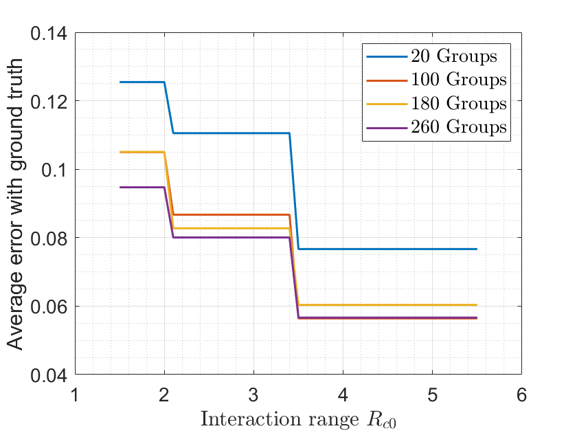
Next, as shown in Fig. 5, the inference performance of the interaction range is evaluated. Since the active excitation method mainly aims to obtain a lower bound of , here we omit the simulation process of this stage and directly present the inference error under different . For fair comparisons, Fig. 5(a) and 5(b) depict the error curve under noise variance from to using 200 observations, while Fig. 5(c)-5(d) depicts the error curve under observation amount from to with . Note that the average error of the inferred topology with the ground truth is computed as . As we can see, the empirical inference function and the average error is generally decreasing with . This corresponds to the result of Theorem 5 and supports the feasibility of using Algorithm 2 to determine a more accurate . Specifically, the more observations are involved, the smaller the average inference error w.r.t. the ground truth is.
Then, with m, we compare the inference performance without and with the interaction constraint, corresponding to and (55), respectively. Fig. 6(a) presents the inference errors under different variances of observation noises, varying from 0 to 0.5. Each test is based on 200 observations over the same time window. Fig. 6(b) presents the inference errors under different number of observations, ranging from 20 to 260, with . Note that all the error indexes (Y-coordinate) in the figures describe the absolute deviation between two variables instead of the relative. Under the same observation amount, the larger is, the less improvement can be obtained. When and are not very large, remarkable improvements in the inference performance can be achieved. In addition, as shown in Fig. 6(b), the inference error can be further reduced with a larger available observation amount (i.e., ), which corresponds to the conclusion of Theorem 4.
Finally, we present the performance comparison of the proposed approach with the methods in [24] and [26] (denoted as M-1 and M-2, respectively), under the same settings of , noise variance and observation amount as the last experiment. Note that for fair comparisons, we use the filtered observations to implement M-1. Fig. 7(a) shows the relationships between the inference error and the observation noise variance for all methods. Fig. 7(b) shows the relationships between the inference error and the observation amount for all methods, under common noise variance . It is clear from the presented results that the proposed method outperforms the other two, which mainly results from the estimation of the formation input and the interaction range. We also observe that the reason for M-1 having better performance than M-2 lies in the filtered observations we used. More detailed technical comparisons along with some other inference algorithms are summarized in Table II. From this table, it shows that the proposed method has better applicability for the considered problem and inference performance guarantees.


| Method | Topology Structure | Input Consideration |
|
Input Filtering | Observation Noise | Convergence Speed | ||||
| Undirected | Directed | Random | Non-random | Feasibility | Conditions | |||||
| Truncated estimator in [24] | Erdős-Rényi graph | |||||||||
| Spectral method in [57] | ||||||||||
| Geometric method in [7] | Binary judgement | Non-steady trajectory is available | No guarantee | |||||||
| OLS-based method in [26] | Feasible if revised | Non-steady trajectory is available | No guarantee | |||||||
| Our method | Non-steady trajectory is available | |||||||||
- 1
and represent the cardinality of the observable subset and the whole node set, respectively.
- 2
here refers to the number of observations in the non-steady stage, and the system in this reference is asymptotically stable.
- 3
In [57] the authors implement groups of tests over the system, with the same initial state while ending at different moments, and no noise terms are involved.
- 4
The method is based on the geometric characteristics of the robot trajectory. Although not tailored for the local topology inference of MRNs, but we point out it can applied to infer whether the connection between two robots exists.
- 5
The method is originally designed for global topology inference, and can be revised for the local cases if using the idea in this paper.
VII Conclusion
In this paper, we have studied the problem of inferring the local topology of MRNs under first-order formation control, without the knowledge about formation input and interaction parameters. To overcome the inference challenges brought by the unknown formation input and interaction range, we first demonstrated how to determine the available robot subset for inference, considering the set of robots that are within the observation range of the inference robot might change over time. Then, we designed -steady pattern estimators to obtain the input parameters and an active excitation method to estimate the interaction range. Then, we proposed a range-shrink strategy to avoid the inference brought by the unobservable robots and presented the local topology estimator. The convergence rate and the accuracy of the proposed estimator were proved. Extensions on different observation slots for the robots and more complicated control models were also analyzed. Finally, extensive simulation tests and comparisons verified the effectiveness of the proposed method. Future directions include i) generalizing the method to more complex formation control cases (e.g., switching topology and nonlinear dynamics); ii) investigating the possible attack against the MRNs based on the inferred topology along with its countermeasures.
-A Proof of Theorem 1
Proof.
Based on Lemma 1, when the MRN has reached -steady pattern after , the dynamics (3) is equivalent to
| (60) |
where , satisfying . Then, the estimation error of is given by
| (61) |
For ease notation, define
| (62) |
Then, we only need to prove the upper bound of
Note that i.i.d., and thus is subject to . Based the Gaussian nature, one can obtain the following concentration inequality by finding the optimal Chernoff bound of (see example 2.1 in [58]), i.e.,
| (63) |
As for , since the system is in -steady pattern, one has
| (64) |
Hence, combining (63) and (64) yields that
| (65) |
Substituting the absolute inequality into (65), the first statement (16) is proved.
Next, consider the estimation error of . Based on (60), one has
| (66) |
Similar with , the average estimation of all elements in (66) is given by
| (67) |
where and . Taking and into the third term , one obtains
| (68) |
Substituting (68) into (67), then one has where
Utilizing and , one deduces that
| (69) | ||||
| (70) |
Combining (69) and (70), it yields that and holds. When , the second statement (17) is proved. ∎
-B Proof of Theorem 2
Proof.
To begin with, similar with (IV-D), the accumulated velocity prediction error is expanded as
| (71) |
where represents the -power of .
Then, it follows that the average velocity prediction error in the -period is given by
| (72) |
Note that is subject to . Applying the Chernoff concentration inequality, one obtains
| (73) |
Recall that it is proved that in Theorem 1, and always holds. Combining these pieces, if is under no excitation (i.e., ), it yields that
| (74) |
Taking the converse-negative version of the statement (i.e., if then (74) holds), it yields the statement described by (39). The proof is completed. ∎
-C Proof of Theorem 4
Proof.
For notational brevity, let be the error vector of the filtered input. Then, for each pair of , we have
| (75) |
Let , and . Then, all the filtered observations can be compactly written as
| (76) |
Based on the estimator (45), the inference error matrix of is given by
| (77) |
Next, we will prove that each term of the RHS of (-C) is bounded individually.
- •
Part 1: Upper Bounding .
Recall that the system state can be expanded recursively as
| (78) |
Note that the last two terms in the RHS of (-C) is strictly bounded regardless of the moment , and the influence of the independent observation noises will not accumulate during the state evolution. Since the term takes the dominant role in the state evolution, we can directly characterize in terms of the time horizon .
Based on the matrix norm inequality , one easily infers that
| (79) |
Further utilizing and , one deduces that . Then, it follows that
| (80) |
By (80), one can always find a group of , such that . In turn, the inverse matrix of satisfies
| (81) |
where the invertibility of is guaranteed by the i.i.d. noise . Therefore, the spectral norm of is characterized by
| (82) |
- •
Part 2: Upper Bounding .
Utilizing the concentration measure in Gaussian space [59], given a random matrix with independent standard normal entries, one has with probability at least
| (83) |
Let and utilize , one has with probability at least that . Note that the observation matrix contains the noise matrix , i.e., . Therefore, it yields that with probability at least
| (84) |
- •
Part 3: Upper Bounding .
Recall that , it can be split as
| (85) |
where and . Then, the upper bound of is given by
| (86) |
By the conclusion of Theorem 1, with probability at least , one has and
| (87) |
Note that Theorem 1 demonstrates that each term in is a random variable of -level mean and -level variance, and thus one deduces that with probability at least
| (88) |
Combining (87) and (88), one obtains
| (89) |
-D Proof of Theorem 5
Proof.
To begin with, suppose and the observations are noise-free for ease notation. Denote by the robot set that is within the range , and define . Then, the filtered observations of satisfy
| (91) |
where . Note that is a -dimension vector. There exists at least a -dimension matrix , such that
| (92) |
Then, substitute (92) into (91) and it yields
| (93) |
Taking the observation noises into account, the OLS estimator of with observations and is given by
| (94) |
Next, applying Theorem 4 on , it yields that
| (95) |
It is straightforward to infer that, if some in-neighbors of are in , then . Therefore, for the local topology estimator , the asymptotic inference bias is given by
| (96) |
For , the cardinal numbers of and satisfy , which indicates that is less biased from the real . The monotone decreasing property of is proved.
Specifically, if , the set . Finally, it follows that and , i.e., is asymptotically unbiased. The proof is completed. ∎
References
- [1] Y. Li, J. He, and C. Lin, “Topology inference on partially observable mobile robotic networks under formation control,” in 2021 European Control Conference (ECC). IEEE, 2021, pp. 497–502.
- [2] F. Bullo, J. Cortes, and S. Martinez, Distributed control of robotic networks: A mathematical approach to motion coordination algorithms. Princeton University Press, 2009, vol. 27.
- [3] R. Olfati-Saber and R. M. Murray, “Consensus problems in networks of agents with switching topology and time-delays,” IEEE Transactions on Automatic Control, vol. 49, no. 9, pp. 1520–1533, 2004.
- [4] K.-K. Oh, M.-C. Park, and H.-S. Ahn, “A survey of multi-agent formation control,” Automatica, vol. 53, pp. 424–440, 2015.
- [5] M. A. Kamel, X. Yu, and Y. Zhang, “Formation control and coordination of multiple unmanned ground vehicles in normal and faulty situations: A review,” Annual Reviews in Control, vol. 49, pp. 128–144, 2020.
- [6] D. Zhang and J. P. Sterbenz, “Analysis of critical node attacks in mobile ad hoc networks,” in 2014 6th International Workshop on Reliable Networks Design and Modeling, 2014, pp. 171–178.
- [7] B. L. M. Vásquez and J. Carlo Barca, “Network topology inference in swarm robotics,” in IEEE International Conference on Robotics and Automation (ICRA). IEEE, 2018, pp. 7660–7666.
- [8] H. Choi, W.-C. Lee, Y. Aafer, F. Fei, Z. Tu, X. Zhang, D. Xu, and X. Xinyan, “Detecting attacks against robotic vehicles: A control invariant approach,” in Proceedings of the 2018 ACM SIGSAC Conference on Computer and Communications Security. ACM, 2018, pp. 801–816.
- [9] Y. Li, J. He, C. Chen, and X. Guan, “Learning-based intelligent attack against formation control with obstacle-avoidance,” in 2019 American Control Conference (ACC). IEEE, 2019, pp. 2690–2695.
- [10] R. A. Licitra, Z. I. Bell, and W. E. Dixon, “Single-agent indirect herding of multiple targets with uncertain dynamics,” IEEE Transactions on Robotics, vol. 35, no. 4, pp. 847–860, 2019.
- [11] J. Li, J. He, Y. Li, and X. Guan, “Unpredictable trajectory design for mobile agents,” in 2020 American Control Conference (ACC). IEEE, 2020, pp. 1471–1476.
- [12] A. Venkitaraman, S. Chatterjee, and B. Wahlberg, “Recursive prediction of graph signals with incoming nodes,” in 2020 IEEE International Conference on Acoustics, Speech and Signal Processing (ICASSP), 2020, pp. 5565–5569.
- [13] Y. Li, H. Wang, J. He, and X. Guan, “Optimal topology recovery scheme for multi-robot formation control,” in IEEE 28th International Symposium on Industrial Electronics (ISIE). IEEE, 2019, pp. 1847–1852.
- [14] D. Deka, S. Backhaus, and M. Chertkov, “Learning topology of the power distribution grid with and without missing data,” in 2016 European Control Conference (ECC). IEEE, 2016, pp. 313–320.
- [15] S. Shi, G. Bottegal, and P. M. Van den Hof, “Bayesian topology identification of linear dynamic networks,” in 2019 European Control Conference (ECC). IEEE, 2019, pp. 2814–2819.
- [16] F. Lu, M. Zhong, S. Tang, and M. Maggioni, “Nonparametric inference of interaction laws in systems of agents from trajectory data,” Proceedings of the National Academy of Sciences, vol. 116, no. 29, pp. 14 424–14 433, 2019.
- [17] X. Dong, D. Thanou, M. Rabbat, and P. Frossard, “Learning graphs from data: A signal representation perspective,” IEEE Signal Processing Magazine, vol. 36, no. 3, pp. 44–63, 2019.
- [18] S. Shahrampour and V. M. Preciado, “Reconstruction of directed networks from consensus dynamics,” in 2013 American Control Conference. IEEE, 2013, pp. 1685–1690.
- [19] ——, “Topology identification of directed dynamical networks via power spectral analysis,” IEEE Transactions on Automatic Control, vol. 60, no. 8, pp. 2260–2265, 2014.
- [20] S. Hassan-Moghaddam, N. K. Dhingra, and M. R. Jovanović, “Topology identification of undirected consensus networks via sparse inverse covariance estimation,” in 2016 IEEE 55th Conference on Decision and Control (CDC). IEEE, 2016, pp. 4624–4629.
- [21] G. Mateos, S. Segarra, A. G. Marques, and A. Ribeiro, “Connecting the dots: Identifying network structure via graph signal processing,” IEEE Signal Processing Magazine, vol. 36, no. 3, pp. 16–43, 2019.
- [22] A. S. Bazanella, M. Gevers, and J. M. Hendrickx, “Network identification with partial excitation and measurement,” in 2019 IEEE 58th Conference on Decision and Control (CDC). IEEE, 2019, pp. 5500–5506.
- [23] H. J. van Waarde, P. Tesi, and M. K. Camlibel, “Topology identification of heterogeneous networks: Identifiability and reconstruction,” Automatica, vol. 123, p. 109331, 2021.
- [24] V. Matta and A. H. Sayed, “Consistent tomography under partial observations over adaptive networks,” IEEE Transactions on Information Theory, vol. 65, no. 1, pp. 622–646, 2019.
- [25] M. Coutino, E. Isufi, T. Maehara, and G. Leus, “State-space network topology identification from partial observations,” IEEE Transactions on Signal and Information Processing over Networks, vol. 6, pp. 211–225, 2020.
- [26] C. Liu, J. He, S. Zhu, and C. Chen, “Dynamic topology inference via external observation for multi-robot formation control,” in 2019 IEEE Pacific Rim Conference on Communications, Computers and Signal Processing (PACRIM), 2019, pp. 1–6.
- [27] C. W. Reynolds, “Flocks, herds and schools: A distributed behavioral model,” in Proceedings of the 14th Annual Conference on Computer Graphics and Interactive Techniques, 1987, pp. 25–34.
- [28] X. Sun and C. G. Cassandras, “Optimal dynamic formation control of multi-agent systems in constrained environments,” Automatica, vol. 73, pp. 169–179, 2016.
- [29] S. Zhao, “Affine formation maneuver control of multiagent systems,” IEEE Transactions on Automatic Control, vol. 63, no. 12, pp. 4140–4155, 2018.
- [30] J. Alonso-Mora, E. Montijano, T. Nägeli, O. Hilliges, M. Schwager, and D. Rus, “Distributed multi-robot formation control in dynamic environments,” Autonomous Robots, vol. 43, no. 5, pp. 1079–1100, 2019.
- [31] Y. Xu, S. Zhao, D. Luo, and Y. You, “Affine formation maneuver control of high-order multi-agent systems over directed networks,” Automatica, vol. 118, p. 109004, 2020.
- [32] M. Deghat, I. Shames, B. D. O. Anderson, and C. Yu, “Localization and circumnavigation of a slowly moving target using bearing measurements,” IEEE Transactions on Automatic Control, vol. 59, no. 8, pp. 2182–2188, 2014.
- [33] T.-H. Cheng, Z. Kan, J. R. Klotz, J. M. Shea, and W. E. Dixon, “Event-triggered control of multiagent systems for fixed and time-varying network topologies,” IEEE Transactions on Automatic Control, vol. 62, no. 10, pp. 5365–5371, 2017.
- [34] M. H. Trinh, S. Zhao, Z. Sun, D. Zelazo, B. D. O. Anderson, and H.-S. Ahn, “Bearing-based formation control of a group of agents with leader-first follower structure,” IEEE Transactions on Automatic Control, vol. 64, no. 2, pp. 598–613, 2018.
- [35] Z. Kan, A. P. Dani, J. M. Shea, and W. E. Dixon, “Network connectivity preserving formation stabilization and obstacle avoidance via a decentralized controller,” IEEE Transactions on Automatic Control, vol. 57, no. 7, pp. 1827–1832, 2012.
- [36] S. Zhao, Z. Li, and Z. Ding, “Bearing-only formation tracking control of multiagent systems,” IEEE Transactions on Automatic Control, vol. 64, no. 11, pp. 4541–4554, 2019.
- [37] C. W. Granger, “Investigating causal relations by econometric models and cross-spectral methods,” Econometrica: Journal of the Econometric Society, pp. 424–438, 1969.
- [38] A. Brovelli, M. Ding, A. Ledberg, Y. Chen, R. Nakamura, and S. L. Bressler, “Beta oscillations in a large-scale sensorimotor cortical network: Directional influences revealed by granger causality,” Proceedings of the National Academy of Sciences, vol. 101, no. 26, pp. 9849–9854, 2004.
- [39] M. Timme, “Revealing network connectivity from response dynamics,” Physical Review Letters, vol. 98, no. 22, p. 224101, 2007.
- [40] W.-X. Wang, Y.-C. Lai, C. Grebogi, and J. Ye, “Network reconstruction based on evolutionary-game data via compressive sensing,” Physical Review X, vol. 1, no. 2, p. 021021, 2011.
- [41] D. Hayden, Y. H. Chang, J. Goncalves, and C. J. Tomlin, “Sparse network identifiability via compressed sensing,” Automatica, vol. 68, pp. 9–17, 2016.
- [42] H.-T. Wai, A. Scaglione, B. Barzel, and A. Leshem, “Joint network topology and dynamics recovery from perturbed stationary points,” IEEE Transactions on Signal Processing, vol. 67, no. 17, pp. 4582–4596, 2019.
- [43] J. Mei and J. M. Moura, “Signal processing on graphs: Modeling (causal) relations in big data,” arXiv preprint arXiv:1503.00173, vol. 1, 2015.
- [44] M. Onuki, S. Ono, M. Yamagishi, and Y. Tanaka, “Graph signal denoising via trilateral filter on graph spectral domain,” IEEE Transactions on Signal and Information Processing over Networks, vol. 2, no. 2, pp. 137–148, 2016.
- [45] H. E. Egilmez, E. Pavez, and A. Ortega, “Graph learning from data under Laplacian and structural constraints,” IEEE Journal of Selected Topics in Signal Processing, vol. 11, no. 6, pp. 825–841, 2017.
- [46] D. Hallac, Y. Park, S. Boyd, and J. Leskovec, “Network inference via the time-varying graphical Lasso,” in Proceedings of the 23rd ACM SIGKDD International Conference on Knowledge Discovery and Data Mining. ACM, 2017, pp. 205–213.
- [47] B. Pasdeloup, V. Gripon, G. Mercier, D. Pastor, and M. G. Rabbat, “Characterization and inference of graph diffusion processes from observations of stationary signals,” IEEE Transactions on Signal and Information Processing over Networks, vol. 4, no. 3, pp. 481–496, 2018.
- [48] G. Karanikolas, G. B. Giannakis, K. Slavakis, and R. M. Leahy, “Multi-kernel based nonlinear models for connectivity identification of brain networks,” in 2016 IEEE International Conference on Acoustics, Speech and Signal Processing (ICASSP). IEEE, 2016, pp. 6315–6319.
- [49] G. V. Karanikolas, O. Sporns, and G. B. Giannakis, “Multi-kernel change detection for dynamic functional connectivity graphs,” in 2017 51st Asilomar Conference on Signals, Systems, and Computers. IEEE, 2017, pp. 1555–1559.
- [50] S. Wang, E. D. Herzog, I. Z. Kiss, W. J. Schwartz, G. Bloch, M. Sebek, D. Granados-Fuentes, L. Wang, and J.-S. Li, “Inferring dynamic topology for decoding spatiotemporal structures in complex heterogeneous networks,” Proceedings of the National Academy of Sciences, vol. 115, no. 37, pp. 9300–9305, 2018.
- [51] R. Olfati-Saber, J. A. Fax, and R. M. Murray, “Consensus and cooperation in networked multi-agent systems,” Proceedings of the IEEE, vol. 95, no. 1, pp. 215–233, 2007.
- [52] A. Pandey, S. Pandey, and D. R. Parhi, “Mobile robot navigation and obstacle avoidance techniques: A review,” International Robotics and Automation Journal, vol. 2, no. 3, p. 00022, 2017.
- [53] A. Santos, V. Matta, and A. H. Sayed, “Local tomography of large networks under the low-observability regime,” IEEE Transactions on Information Theory, vol. 66, no. 1, pp. 587–613, 2020.
- [54] M. Cirillo, V. Matta, and A. H. Sayed, “Learning Bollobás-Riordan graphs under partial observability,” in 2021 IEEE International Conference on Acoustics, Speech and Signal Processing (ICASSP). IEEE, 2021, pp. 5360–5364.
- [55] S. Boyd, S. P. Boyd, and L. Vandenberghe, Convex optimization. Cambridge university press, 2004.
- [56] Y. Cao and W. Ren, “Sampled-data discrete-time coordination algorithms for double-integrator dynamics under dynamic directed interaction,” International Journal of Control, vol. 83, no. 3, pp. 506–515, 2010.
- [57] Y. Zhu, M. T. Schaub, A. Jadbabaie, and S. Segarra, “Network inference from consensus dynamics with unknown parameters,” IEEE Transactions on Signal and Information Processing over Networks, vol. 6, pp. 300–315, 2020.
- [58] M. J. Wainwright, High-dimensional statistics: A non-asymptotic viewpoint. Cambridge University Press, 2019, vol. 48.
- [59] K. R. Davidson and S. J. Szarek, “Local operator theory, random matrices and banach spaces,” Handbook of the geometry of Banach spaces, vol. 1, no. 317-366, p. 131, 2001.
| Yushan Li (S’19) received the B.E. degree in School of Artificial Intelligence and Automation from Huazhong University of Science and Technology, Wuhan, China, in 2018. He is currently working toward the Ph.D. degree with the Dept. of Automation, Shanghai Jiaotong University, Shanghai, China. He is a member of Intelligent of Wireless Networking and Cooperative Control group. His research interests include robotics, security of cyber-physical system, and distributed computation and optimization in multi-agent networks. |
| Jianping He (SM’19) is currently an associate professor in the Department of Automation at Shanghai Jiao Tong University. He received the Ph.D. degree in control science and engineering from Zhejiang University, Hangzhou, China, in 2013, and had been a research fellow in the Department of Electrical and Computer Engineering at University of Victoria, Canada, from Dec. 2013 to Mar. 2017. His research interests mainly include the distributed learning, control and optimization, security and privacy in network systems. Dr. He serves as an Associate Editor for IEEE Open Journal of Vehicular Technology and KSII Trans. Internet and Information Systems. He was also a Guest Editor of IEEE TAC, International Journal of Robust and Nonlinear Control, etc. He was the winner of Outstanding Thesis Award, Chinese Association of Automation, 2015. He received the best paper award from IEEE WCSP’17, the best conference paper award from IEEE PESGM’17, and was a finalist for the best student paper award from IEEE ICCA’17. |
| Cai Lin (F’20) received the M.A.Sc. and Ph.D. degrees (awarded Outstanding Achievement in Graduate Studies) in electrical and computer engineering from the University of Waterloo, Waterloo, Canada, in 2002 and 2005, respectively. Since 2005, she has been with the Department of Electrical and Computer Engineering at the University of Victoria, where she is currently a Professor. She is an NSERC E.W.R. Steacie Memorial Fellow. Her research interests span several areas in communications and networking, with a focus on network protocol and architecture design supporting emerging multimedia traffic and the Internet of Things. She was a recipient of the NSERC Discovery Accelerator Supplement (DAS) Grants in 2010 and 2015, respectively, and the best paper awards of IEEE ICC 2008 and IEEE WCNC 2011. She has co-founded and chaired the IEEE Victoria Section Vehicular Technology and Communications Joint Societies Chapter. She has been elected to serve the IEEE Vehicular Technology Society Board of Governors, 2019 - 2021. She has served as an Area Editor for IEEE TRANSACTIONS ON VEHICULAR TECHNOLOGY, a member of the Steering Committee of the IEEE TRANSACTIONS ON BIG DATA (TBD) and IEEE TRANSACTIONS ON CLOUD COMPUTING (TCC), an Associate Editor of the IEEE INTERNET OF THINGS JOURNAL, IEEE TRANSACTIONS ON WIRELESS COMMUNICATIONS, IEEE TRANSACTIONS ON VEHICULAR TECHNOLOGY, IEEE TRANSACTIONS ON COMMUNICATIONS, EURASIP Journal on Wireless Communications and Networking, International Journal of Sensor Networks, and Journal of Communications and Networks (JCN), and as the Distinguished Lecturer of the IEEE VTS Society. She has served as a TPC co-chair for IEEE VTC2020-Fall, and a TPC symposium co-chair for IEEE Globecom’10 and Globecom’13. She is a Registered Professional Engineer in British Columbia, Canada. |
| Xinping Guan (F’18) received the B.S. degree in Mathematics from Harbin Normal University, Harbin, China, in 1986, and the Ph.D. degree in Control Science and Engineering from Harbin Institute of Technology, Harbin, China, in 1999. He is currently a Chair Professor with Shanghai Jiao Tong University, Shanghai, China, where he is the Dean of School of Electronic, Information and Electrical Engineering, and the Director of the Key Laboratory of Systems Control and Information Processing, Ministry of Education of China. Before that, he was the Professor and Dean of Electrical Engineering, Yanshan University, Qinhuangdao, China. Dr. Guan’s current research interests include industrial cyber-physical systems, wireless networking and applications in smart factory, and underwater networks. He has authored and/or coauthored 5 research monographs, more than 270 papers in IEEE Transactions and other peer-reviewed journals, and numerous conference papers. As a Principal Investigator, he has finished/been working on many national key projects. He is the leader of the prestigious Innovative Research Team of the National Natural Science Foundation of China (NSFC). Dr. Guan received the First Prize of Natural Science Award from the Ministry of Education of China in both 2006 and 2016, and the Second Prize of the National Natural Science Award of China in both 2008 and 2018. He was a recipient of IEEE Transactions on Fuzzy Systems Outstanding Paper Award in 2008. He is a National Outstanding Youth honored by NSF of China, Changjiang Scholar by the Ministry of Education of China and State-level Scholar of New Century Bai Qianwan Talent Program of China. |