Tight analytic bound on the trade-off between device-independent randomness and nonlocality
Abstract
Two parties sharing entangled quantum systems can generate correlations that cannot be produced using only shared classical resources. These nonlocal correlations are a fundamental feature of quantum theory but also have practical applications. For instance, they can be used for device-independent (DI) random number generation, whose security is certified independently of the operations performed inside the devices. The amount of certifiable randomness that can be generated from some given non-local correlations is a key quantity of interest. Here we derive tight analytic bounds on the maximum certifiable randomness as a function of the nonlocality as expressed using the Clauser-Horne-Shimony-Holt (CHSH) value. We show that for every CHSH value greater than the local value () and up to there exist quantum correlations with that CHSH value that certify a maximal two bits of global randomness. Beyond this CHSH value the maximum certifiable randomness drops. We give a second family of Bell inequalities for CHSH values above , and show that they certify the maximum possible randomness for the given CHSH value. Our work hence provides an achievable upper bound on the amount of randomness that can be certified for any CHSH value. We illustrate the robustness of our results, and how they could be used to improve randomness generation rates in practice, using a Werner state noise model.
I Introduction
Nonlocality is the phenomenon where measurements of certain quantum systems, by isolated observers, generate correlations inaccessible to any local systems that behave classically Bell 1987; Brunner et al. 2014. Nonlocal correlations can be used to make statements about the underlying quantum system without characterizing the devices used Mayers and Yao 2004; McKague et al. 2012; Yang and Navascués 2013; Kaniewski 2017; Šupić and Bowles 2020, and constitute a resource for information processing Barrett et al. 2005a. In particular, they give rise to the possibility of DI information processing which allows, for instance, the intrinsic randomness of nonlocal correlations to be exploited for randomness expansion Colbeck 2007; Pironio et al. 2010; Colbeck and Kent 2011; Miller and Shi 2014; Miller and Shi 2017a, amplification Colbeck and Renner 2012, and key distribution protocols Ekert 1991; Barrett et al. 2005b; Acin et al. 2007; Pironio et al. 2009; Vazirani and Vidick 2014; Arnon-Friedman et al. 2018.
Given some experimental conditions in a particular input-output scenario, what is the optimal way to generate randomness device-independently? Since the values of extremal Bell inequalities quantify the distance of the observed correlations from the local boundary, one might expect these to be optimal for randomness. However, the relationship between nonlocality and maximum randomness is nontrivial de la Torre et al. 2015, and it has been shown that non-extremal Bell inequalities can certify more randomness in some cases Acín et al. 2012.
A substantial literature has developed investigating the maximum achievable randomness in different DI scenarios. In particular, the existence of Bell tests that can certify maximum global randomness was shown in Dhara et al. 2013 by adding extra measurements. Constructions achieving maximal randomness in the bipartite scenario for non-projective measurements were given in Acín et al. 2016 and for greater than two projective measurements per party in Law et al. 2014; Andersson et al. 2018; Brown et al. 2020; Woodhead et al. 2020. In Acín et al. 2012 a construction that tends towards the maximum 2 random bits is presented, based on the violation of tilted-CHSH inequalities Acín et al. 2012; Bamps and Pironio 2015. This provides a key example where non-extremal Bell inequalities certify more randomness (maximum violation of the CHSH inequality, the only extremal Bell inequality in the 2-input, 2-output scenario up to symmetry, can certify bits of global randomness by comparison — see, e.g., Bhavsar et al. 2021). Based on Acín et al. 2012 one might expect that achieving 2 bits of randomness requires the CHSH violation (or entanglement) of the strategy to tend to . If this were the case, there would be a problem with the robustness of the construction, and the result suggests a trade-off between certifiable randomness and distance from the local set. Ref. Acín et al. 2012 left open whether two bits of randomness is actually attainable using a single statistic in the 2-input 2-output scenario, and how non-local a strategy achieving this can be.
Our work gives conclusive answers to these questions. We consider the maximum amount of DI randomness that can be certified from the set of quantum correlations achieving a particular CHSH value. In other words, we investigate how much randomness is achievable when the generating system is required to exhibit a particular amount of nonlocality. To do so, we introduce two families of Bell expressions that self-test families of two qubit strategies. Our first family (see Proposition 1) certifies exactly 2 random bits for all CHSH values in the interval , showing 2 random bits are achievable without tending towards the local set Acín et al. 2012, requiring extra measurements Brown et al. 2020; Woodhead et al. 2020; Law et al. 2014 or constraining the full distribution Brown et al. 2021. Our second family (see Proposition 2) covers the range of values , coinciding with the CHSH inequality for , and the certifiable randomness achieved is a smooth, monotonically decreasing function of the value. We show in Proposition 3 that this is the true maximum randomness achievable for this range of CHSH values, illustrating how one only needs to sacrifice randomness when approaching the maximum quantum value of CHSH. Finally, we analyse the robustness of our construction under a Werner state noise model Werner 1989, and compare it to that of the tilted CHSH inequalities. We find both constructions to be robust, and at any given noise level there exists an optimal statistic for practical DI randomness generation that can outperform CHSH.
II DI scenario
We consider the bipartite 2-input 2-output Bell scenario. Let two isolated devices each receive an input , from which they produce an output , stored in the classical registers and . The devices are characterised by the joint conditional probability distribution , which, due to the isolation of the devices, must be no-signalling.
We refer to a quantum strategy when the devices share a bipartite density operator on the Hilbert space , and measure observables , where are projective measurements on the associated Hilbert space (projective measurements can be assumed without loss of generality according to Naimark’s dilation theorem Paulsen 2003). We also include the possibility of an adversary Eve, who wishes to guess the outputs. In the DI scenario, Eve may have supplied the devices used by the user (Alice) and may hold a purifying system with associated Hilbert space such that the post-measurement system and are correlated. We describe this using a tripartite density operator, such that . Following measurement with inputs and , we obtain the classical-quantum state , where is proportional to Eve’s state conditioned on the joint measurement outcomes, and the distribution is recovered via .
III Nonlocality and self-tests
To quantify the distance of an observed distribution from the local boundary in this scenario, we consider the CHSH expression , where when admits a quantum representation with purified state and observables . The local bound is given by , and the maximum quantum value is Cirel’son 1980. Any distribution that violates the local bound is said to be nonlocal.
It is known that the CHSH inequality self-tests the maximally entangled state and the measurements that achieve its maximum quantum violation Popescu and Rohrlich 1992; Bardyn et al. 2009; Šupić and Bowles 2020; Bamps and Pironio 2015 in the sense that there is only one state and set of measurements that can achieve up to local isometries. One can also define a robust self test, in which close to maximum violation certifies a state and measurements close to the optimal ones up to local isometries.
IV Entropy bounds
The quantity of interest for calculating the DI global randomness is the conditional von Neumann entropy when the devices receive inputs , , evaluated for the post-measurement state . This is the relevant quantity for spot-checking DI random number generation Bhavsar et al. 2021. For DI randomness expansion we require lower bounds on this quantity that hold for all states and measurements compatible with the observed distribution , or some linear functions of , e.g., the CHSH value. This gives the asymptotic rate of randomness generation , in bits per round:
| (1) |
The asymptotic rate can also be used as a basis for rates with finite statistics using tools such as the entropy accumulation theorem Dupuis et al. 2016; Dupuis and Fawzi 2019; Liu et al. 2021.
In the noiseless scenario, we prove a self-testing statement that certifies a state and measurements that generate two bits of randomness. In this case, is a self-testing Bell expression, and there is only one state and set of measurements that can achieve the maximal quantum value (up to symmetries), from which the conditional entropy can be evaluated. For the noisy case, we use the recently developed numerical technique from Brown et al. 2021 to compute lower bounds on Eq. 1 using semidefinite programming.
V Main results
Our first main result is the family of Bell expressions that works for CHSH values in the range .
Proposition 1.
Let , and define the family of Bell expressions parameterized by , labelled :
| (2) |
Then we have the following:
- (i)
The local bound is given by .
- (ii)
The quantum bound is given by .
- (iii)
Up to local isometries there is a unique strategy that achieves :
(3)
By the previous discussion of the noiseless case, Proposition 1 shows that there exists a family of two-qubit strategies that can achieve exactly two bits of global DI randomness in the bipartite, 2-input 2-output case; this follows from self-testing measurements together with the maximally entangled state . We now explore some implications of this. The strategy in Eq. 3 has a CHSH value and by sweeping the interval of values is achieved. Hence for every CHSH value in this interval, there exists a two-qubit strategy achieving this value, that can certify exactly 2 bits of randomness. In fact is the largest CHSH value for which exactly two bits of randomness can be achieved, corresponding to the strategy in Eq. 3 (see the Supplemental Material Wooltorton et al.). This strategy can be derived by fixing , and optimising the the remaining measurement angles for the maximum CHSH value. This improves upon the results in Acín et al. 2012 (cf. the introduction): rather than needing low CHSH violation to get close to maximal randomness, maximum randomness is achieved well into the nonlocal region.
Next we derive the maximum randomness for strategies achieving a CHSH value in the interval . Up to local isometries, the only strategy that can achieve is given by the maximally entangled state with measurements , , and , since the CHSH inequality self-tests this state and measurements Bamps and Pironio 2015. This strategy gives roughly bits of randomness. There must therefore be a transition between and , where in order to achieve a larger CHSH value, randomness must be sacrificed. This transition is given by the following proposition.
Proposition 2.
Let , and define the family of Bell expressions parameterized by , labelled :
| (4) |
where . Then we have the following:
- (i)
The local bound is given by .
- (ii)
The quantum bound is given by .
- (iii)
Up to local isometries there is a unique strategy that achieves :
(5)
When , this corresponds to the expression in Eq. 2 for , and when we recover the CHSH expression. The CHSH value for this family is given by , and monotonically decreases in the interval . The randomness certified by these self-tests is maximum for each CHSH value, summarized in our final proposition.
Proposition 3.
Propositions 1–3 are proven in the Appendices. In Fig. 1, we illustrate our results and compare them to a reliable lower bound on the minimum amount of randomness guaranteed by the same CHSH value Brown et al. 2021. These two curves represent tight upper and lower bounds on the amount of DI randomness that can be certified by strategies achieving a particular CHSH value.
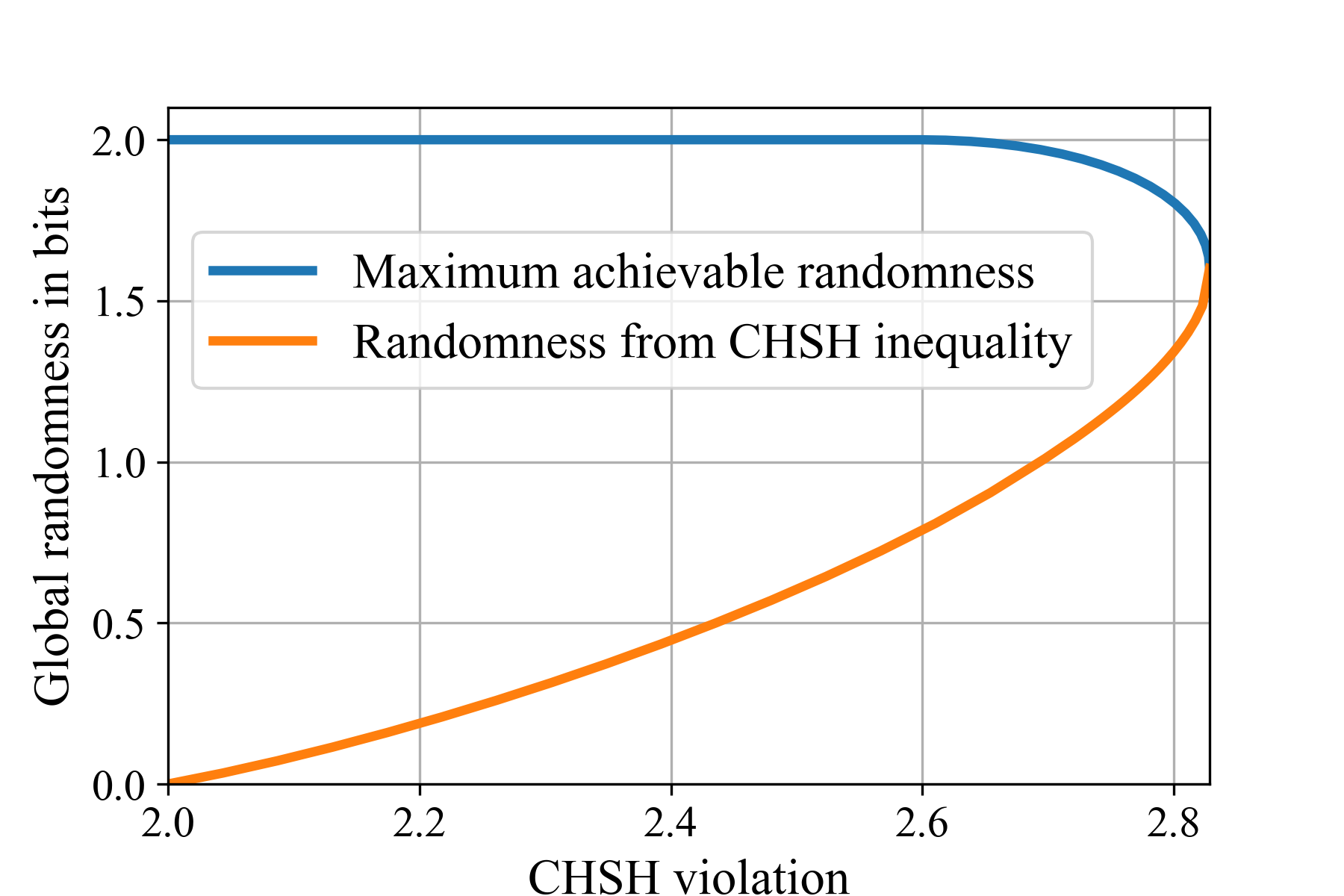
In Fig. 2 we explore the robustness of our constructions. We consider a Werner state noise model Werner 1989, i.e., , where is the weight of the uniform noise. For simplicity, we assume noiseless measurements. We use this state and measurements to simulate statistics from which reliable DI lower bounds can be generated using the techniques of Brown et al. 2021. At each noise level, the randomness is optimized over the choice of self-test from Eq. 4. This is compared to the tilted CHSH expressions Acín et al. 2012; Bamps and Pironio 2015, where the tilting parameter is similarly optimized.

VI Discussion
Our tight upper bound on the achievable DI randomness conditioned on the CHSH value shows that only when one approaches Tsirelson’s bound does one need to sacrifice randomness for nonlocality. This comes from the fact that the optimal measurements needed to achieve have correlated outcomes, whereas correlations that satisfy can have uniform measurement outcomes. When there is zero noise, such a distribution can be used to generate 2 bits of randomness (using the strategy in Eq. 5). As noise is added, using the family of Bell inequalities that self-test a distribution with a CHSH value greater than (obtained by increasing ), we can continue to certify more randomness than would be possible using CHSH inequality at that noise level. Taking the optimal value of at each level of noise we find that the Bell expressions tend to the CHSH statistic as the noise approaches the boundary where no randomness can be certified. In this sense, CHSH is the most robust statistic, which is natural since it defines a facet of the local polytope and so becomes the only Bell inequality that can be violated with high enough noise. We also remark that the robustness of the tilted CHSH inequalities presented here is higher than that of Acín et al. 2012 (cf. the orange vs green curves in Fig. 2). This is a result of using improved numerical techniques to bound the conditional von Neumann entropy directly rather than the min-entropy that is used in Acín et al. 2012.
Based on an experimental estimate of the noise, a Bell inequality from one of our families could be chosen that maximises the certifiable randomness (along the lines of Fig. 2). Knowledge of the full distribution could also boost the noise performance or be used to search for improved protocols in the presence of noise. However, the use of more parameters would lead to a penalty when finite size effects are accounted for. We leave the question of how our construction performs in other noise models, such as detector efficiency, to future work, and pose an open question as to if our construction is truly optimal in the noisy regime.
One other potential application of our constructions is to blind randomness expansion Miller and Shi 2017b; Fu and Miller 2018; Metger et al. 2022, where Alice tries to certify local randomness from one device without trusting the other. Since their outputs are uncorrelated following a self-test from Proposition 1, such a statistic could be used to generate the optimal 1 bit of local randomness in the blind setting.
Finally, it would be interesting to further investigate analogous results in multi-partite scenarios Woodhead et al. 2018; Grasselli et al. 2021 or those with more inputs or outputs Sarkar et al. 2021. Indeed, Grasselli et al. 2021 showed maximal randomness for the outputs of two parties based on a three party Mermin-Ardehali-Belinskii-Klyshko inequality Collins et al. 2002, and with advancements in computational efficiency from new numerical techniques Brown et al. 2021; Masini et al. 2021 alongside self-testing results Mckague 2011; Wu et al. 2014, multi-partite DI-RG has many avenues to explore.
Acknowledgements.
This work was supported by EPSRC via the Quantum Communications Hub (Grant No. EP/T001011/1) and Grant No. EP/SO23607/1.References
- Bell (1987) J. S. Bell, Speakable and unspeakable in quantum mechanics (Cambridge University Press, 1987).
- Brunner et al. (2014) N. Brunner, D. Cavalcanti, S. Pironio, V. Scarani, and S. Wehner, “Bell nonlocality,” Reviews of Modern Physics 86, 419–478 (2014).
- Mayers and Yao (2004) D. Mayers and A. Yao, “Self testing quantum apparatus,” (2004), arXiv:quant-ph/0307205 [quant-ph] .
- McKague et al. (2012) M. McKague, T. H. Yang, and V. Scarani, “Robust self-testing of the singlet,” Journal of Physics A: Mathematical and Theoretical 45, 455304 (2012).
- Yang and Navascués (2013) T. H. Yang and M. Navascués, “Robust self-testing of unknown quantum systems into any entangled two-qubit states,” Physical Review A 87, 050102 (2013).
- Kaniewski (2017) J. Kaniewski, “Self-testing of binary observables based on commutation,” Physical Review A 95, 062323 (2017).
- Šupić and Bowles (2020) I. Šupić and J. Bowles, “Self-testing of quantum systems: a review,” Quantum 4, 337 (2020).
- Barrett et al. (2005a) J. Barrett, N. Linden, S. Massar, S. Pironio, S. Popescu, and D. Roberts, “Nonlocal correlations as an information-theoretic resource,” Physical Review A 71, 022101 (2005a).
- Colbeck (2007) R. Colbeck, Quantum and Relativistic Protocols For Secure Multi-Party Computation, Ph.D. thesis, University of Cambridge (2007), also available as arXiv:0911.3814.
- Pironio et al. (2010) S. Pironio, A. Acin, S. Massar, A. Boyer de la Giroday, D. N. Matsukevich, P. Maunz, S. Olmschenk, D. Hayes, L. Luo, T. A. Manning, and C. Monroe, “Random numbers certified by Bell’s theorem,” Nature 464, 1021–1024 (2010).
- Colbeck and Kent (2011) R. Colbeck and A. Kent, “Private randomness expansion with untrusted devices,” Journal of Physics A 44, 095305 (2011).
- Miller and Shi (2014) C. A. Miller and Y. Shi, “Robust protocols for securely expanding randomness and distributing keys using untrusted quantum devices,” in Proceedings of the 46th Annual ACM Symposium on Theory of Computing, STOC ’14 (ACM, New York, NY, USA, 2014) pp. 417–426.
- Miller and Shi (2017a) C. A. Miller and Y. Shi, “Universal security for randomness expansion from the spot-checking protocol,” SIAM Journal of Computing 46, 1304–1335 (2017a).
- Colbeck and Renner (2012) R. Colbeck and R. Renner, “Free randomness can be amplified,” Nature Physics 8, 450–454 (2012).
- Ekert (1991) A. K. Ekert, “Quantum cryptography based on Bell’s theorem,” Physical Review Letters 67, 661–663 (1991).
- Barrett et al. (2005b) J. Barrett, L. Hardy, and A. Kent, “No signalling and quantum key distribution,” Physical Review Letters 95, 010503 (2005b).
- Acin et al. (2007) A. Acin, N. Brunner, N. Gisin, S. Massar, S. Pironio, and V. Scarani, “Device-independent security of quantum cryptography against collective attacks,” Physical Review Letters 98, 230501 (2007).
- Pironio et al. (2009) S. Pironio, A. Acin, N. Brunner, N. Gisin, S. Massar, and V. Scarani, “Device-independent quantum key distribution secure against collective attacks,” New Journal of Physics 11, 045021 (2009).
- Vazirani and Vidick (2014) U. Vazirani and T. Vidick, “Fully device-independent quantum key distribution,” Physical Review Letters 113, 140501 (2014).
- Arnon-Friedman et al. (2018) R. Arnon-Friedman, F. Dupuis, O. Fawzi, R. Renner, and T. Vidick, “Practical device-independent quantum cryptography via entropy accumulation,” Nature communications 9, 459 (2018).
- de la Torre et al. (2015) G. de la Torre, M. J. Hoban, C. Dhara, G. Prettico, and A. Acín, “Maximally nonlocal theories cannot be maximally random,” Physical Review Letters 114, 160502 (2015).
- Acín et al. (2012) A. Acín, S. Massar, and S. Pironio, “Randomness versus nonlocality and entanglement,” Physical Review Letters 108, 100402 (2012).
- Dhara et al. (2013) C. Dhara, G. Prettico, and A. Acín, “Maximal quantum randomness in Bell tests,” Physical Review A 88, 052116 (2013).
- Acín et al. (2016) A. Acín, S. Pironio, T. Vértesi, and P. Wittek, “Optimal randomness certification from one entangled bit,” Physical Review A 93, 040102 (2016).
- Law et al. (2014) Y. Z. Law, L. P. Thinh, J.-D. Bancal, and V. Scarani, “Quantum randomness extraction for various levels of characterization of the devices,” Journal of Physics A: Mathematical and Theoretical 47, 424028 (2014).
- Andersson et al. (2018) O. Andersson, P. Badziąg, I. Dumitru, and A. Cabello, “Device-independent certification of two bits of randomness from one entangled bit and gisin’s elegant bell inequality,” Phys. Rev. A 97, 012314 (2018).
- Brown et al. (2020) P. J. Brown, S. Ragy, and R. Colbeck, “A framework for quantum-secure device-independent randomness expansion,” IEEE Transactions on Information Theory 66, 2964–2987 (2020).
- Woodhead et al. (2020) E. Woodhead, J. Kaniewski, B. Bourdoncle, A. Salavrakos, J. Bowles, A. Acín, and R. Augusiak, “Maximal randomness from partially entangled states,” Physical Review Research 2, 042028 (2020).
- Bamps and Pironio (2015) C. Bamps and S. Pironio, “Sum-of-squares decompositions for a family of Clauser-Horne-Shimony-Holt-like inequalities and their application to self-testing,” Physical Review A 91, 052111 (2015).
- Bhavsar et al. (2021) R. Bhavsar, S. Ragy, and R. Colbeck, “Improved device-independent randomness expansion rates from tight bounds on the two sided randomness using CHSH tests,” (2021), arXiv:2103.07504 [quant-ph] .
- Brown et al. (2021) P. Brown, H. Fawzi, and O. Fawzi, “Device-independent lower bounds on the conditional von Neumann entropy,” (2021), arXiv:2106.13692 [quant-ph] .
- Werner (1989) R. F. Werner, “Quantum states with Einstein-Podolsky-Rosen correlations admitting a hidden-variable model,” Physical Review A 40, 4277–4281 (1989).
- Paulsen (2003) V. Paulsen, Completely Bounded Maps and Operator Algebras, Cambridge Studies in Advanced Mathematics (Cambridge University Press, 2003).
- Cirel’son (1980) B. Cirel’son, “Quantum generalizations of Bell’s inequality,” Letters in Mathematical Physics 4, 93–100 (1980).
- Popescu and Rohrlich (1992) S. Popescu and D. Rohrlich, “Which states violate Bell’s inequality maximally?” Physics Letters A 169, 411–414 (1992).
- Bardyn et al. (2009) C.-E. Bardyn, T. C. H. Liew, S. Massar, M. McKague, and V. Scarani, “Device-independent state estimation based on Bell’s inequalities,” Physical Review A 80, 062327 (2009).
- Dupuis et al. (2016) F. Dupuis, O. Fawzi, and R. Renner, “Entropy accumulation,” e-print arXiv:1607.01796 (2016).
- Dupuis and Fawzi (2019) F. Dupuis and O. Fawzi, “Entropy accumulation with improved second-order term,” IEEE Transactions on Information Theory 65, 7596–7612 (2019).
- Liu et al. (2021) W.-Z. Liu, M.-H. Li, S. Ragy, S.-R. Zhao, B. Bai, Y. Liu, P. J. Brown, J. Zhang, R. Colbeck, J. Fan, Q. Zhang, and J.-W. Pan, “Device-independent randomness expansion against quantum side information,” Nature Physics 17, 448–451 (2021).
- (40) L. Wooltorton, P. Brown, and R. Colbeck, Supplemental Material containing proofs of the propositions and including additional references Jordan 1875; Goh et al. 2018; Sekatski et al. 2018; Valcarce et al. 2022.
- Miller and Shi (2017b) C. A. Miller and Y. Shi, “Randomness in nonlocal games between mistrustful players,” Quantum information & computation 17, 595–610 (2017b).
- Fu and Miller (2018) H. Fu and C. A. Miller, “Local randomness: Examples and application,” Physical Review A 97, 032324 (2018).
- Metger et al. (2022) T. Metger, O. Fawzi, D. Sutter, and R. Renner, “Generalised entropy accumulation,” (2022), arXiv:2203.04989 [quant-ph] .
- Woodhead et al. (2018) E. Woodhead, B. Bourdoncle, and A. Acín, “Randomness versus nonlocality in the Mermin-Bell experiment with three parties,” Quantum 2, 82 (2018).
- Grasselli et al. (2021) F. Grasselli, G. Murta, H. Kampermann, and D. Bruß, “Entropy bounds for multiparty device-independent cryptography,” PRX Quantum 2, 010308 (2021).
- Sarkar et al. (2021) S. Sarkar, D. Saha, J. Kaniewski, and R. Augusiak, “Self-testing quantum systems of arbitrary local dimension with minimal number of measurements,” npj Quantum Information 7, 151 (2021).
- Collins et al. (2002) D. Collins, N. Gisin, S. Popescu, D. Roberts, and V. Scarani, “Bell-type inequalities to detect true -body nonseparability,” Physical Review Letters 88, 170405 (2002).
- Masini et al. (2021) M. Masini, S. Pironio, and E. Woodhead, “Simple and practical DIQKD security analysis via BB84-type uncertainty relations and pauli correlation constraints,” (2021), arXiv:2107.08894 [quant-ph] .
- Mckague (2011) M. Mckague, “Self-testing graph states,” in Revised Selected Papers of the 6th Conference on Theory of Quantum Computation, Communication, and Cryptography - Volume 6745, TQC 2011 (Springer-Verlag, Berlin, Heidelberg, 2011) p. 104–120.
- Wu et al. (2014) X. Wu, Y. Cai, T. H. Yang, H. N. Le, J.-D. Bancal, and V. Scarani, “Robust self-testing of the three-qubit W state,” Physical Review A 90, 042339 (2014).
- Jordan (1875) C. Jordan, “Essai sur la géométrie à n dimensions,” Bulletin de la S. M. F. 3, 103–174 (1875).
- Goh et al. (2018) K. T. Goh, J. Kaniewski, E. Wolfe, T. Vértesi, X. Wu, Y. Cai, Y.-C. Liang, and V. Scarani, “Geometry of the set of quantum correlations,” Physical Review A 97, 022104 (2018).
- Sekatski et al. (2018) P. Sekatski, J.-D. Bancal, S. Wagner, and N. Sangouard, “Certifying the building blocks of quantum computers from Bell’s theorem,” Physical Review Letters 121, 180505 (2018).
- Valcarce et al. (2022) X. Valcarce, J. Zivy, N. Sangouard, and P. Sekatski, “Self-testing two-qubit maximally entangled states from generalized Clauser-Horne-Shimony-Holt tests,” Physical Review Research 4, 013049 (2022).
Appendix A Proof of Propositions 1 and 2
Proposition 1 (-family of self-tests). Let , and define the family of Bell expressions parameterized by ,
| (7) |
Then we have the following:
- (i)
The local bound is given by .
- (ii)
The quantum bound is given by .
- (iii)
Up to local isometries there is a unique strategy that achieves :
(8)
Proposition 2 (-family of self-tests). Let , and define the family of Bell expressions parameterized by ,
| (9) |
Then we have the following:
- (i)
The local bound is given by .
- (ii)
The quantum bound is given by .
- (iii)
Up to local isometries there is a unique strategy that achieves :
(10)
We follow the same method for both cases. For part , the local bound can be found by setting the observables to , corresponding to an extremal or deterministic strategy. Since these are the vertices of the local polytope, one such combination will be the optimal local strategy.
For the quantum bound in part , a sum-of-squares (SOS) decomposition is found for the Bell expression offset by its claimed maximum quantum value, exploiting the symmetry of the Bell expression under relabelling of and Bamps and Pironio 2015. The existence of an SOS decomposition proves the maximum quantum value claimed, and is detailed in Sections A.1 and A.2.
For the self-test in part we use the resulting SOS decomposition in combination with Jordan’s lemma Jordan 1875. This simplifies the analysis to qubits, and we derive a system of non-linear equations satisfied by any state and measurements that achieve the maximum quantum value. The resulting system is then analytically solved, and we show the only state and measurements for which these equations are satisfied is given by the target strategy (Eqs. 8 and 10) up to local unitaries. This process is detailed in Sections A.3, A.4 and A.5, and completes the proof of Propositions 1 and 2. We remark that our self-tests define hyperplanes tangential to the corresponding strategy on the boundary of the quantum set Goh et al. 2018.
For completeness, in Section A.6, we show from Jordan’s lemma that the private randomness of any strategy that saturates the quantum bounds in Propositions 1 and 2 is equal to that of the target strategy.
A.1 Self-testing and sum-of-squares decompositions
We consider only the exact self-testing statement in this work, and leave proof of the robust statement for future work. We begin by defining self-testing.
Definition 1 (Self-test).
Let the observables , and pure state be the target two-qubit strategy, and let be a Bell operator. The inequality self-tests the target state and measurements if for all physical quantum strategies that satisfy , there exists a local isometry , , and ancillary state such that, for the purification of ,
| (11) |
Throughout this appendix, we refer to the physical state and measurements we are trying to self-test as the “reference”, denoted with a tilde. The strategies in Eqs. 8 and 10 are then the “target” state and measurements; which target strategy we refer to will be clear from the context.
For a Bell operator that defines the quantum Bell inequality , the operator , satisfies for all quantum states , i.e., . If there exists a set of operators that are polynomials of and satisfy
| (12) |
then we have found a sum-of-squares (SOS) decomposition of the operator : positivity of follows directly from the fact that for any operator .
SOS decompositions can be used to enforce algebraic constraints on any state and measurements that satisfy , since this implies
| (13) |
This can only hold if for all . Relations of this form are used to prove the self-testing statement in Eq. 11.
A.2 SOS decomposition for the inequalities in Propositions 1 and 2
Finding an SOS decomposition can be recast as a semidefinite program (SDP) Bamps and Pironio 2015. We start by considering a vector whose components are linear combinations of , , and . We consider the case where each polynomial is linear, writing for some coefficients . Then
| (14) |
where is the Gram matrix of the set of vectors . Since is a Gram matrix, it is positive semidefinite by construction. We can hence use semidefinite programming to find an that satisfies Eq. 14, and then find the polynomials via the matrix square root:
| (15) |
Since each entry of the vector takes the form , we find that provides the set of polynomials that satisfies Eq. 14.
For the Bell operator , where
| (16) |
the SOS decomposition is given by the following lemma.
Lemma 1 (-family SOS decomposition).
Let , where
| (17) | |||
| (18) | |||
| (19) | |||
| (20) |
For every , the Bell expressions can be written as a SOS decomposition where
| (21) |
for , and .
The maximum quantum value of is .
Proof.
The claim can be verified by direct calculation. Since we have , but the quantum strategy given in (8) shows that this bound is achievable. ∎
Four polynomials emerge from this decomposition:
| (22) | ||||
| (23) | ||||
| (24) | ||||
| (25) |
where
| (26) |
Similarly, the shifted Bell operator for the family is given by , where
| (27) |
and we have the following SOS decomposition:
Lemma 2 (-family SOS decomposition).
Let be as defined in Lemma 1. For every , the Bell expressions can be written as a SOS decomposition where
| (28) |
where .
The maximum quantum value of is .
This can be proven in exactly the same way as Lemma 1 and gives rise to the polynomials
| (29) | ||||
| (30) | ||||
| (31) | ||||
| (32) |
where
| (33) |
A.3 Applying Jordan’s lemma
We can use the polynomials derived above for both families of inequalities to impose algebraic constraints on the state and measurements that satisfy . We employ Jordan’s lemma Jordan 1875, a unique simplification that can be made in the 2-input 2-output scenario Pironio et al. 2009; Bhavsar et al. 2021. The lemma states that for two observables and on a Hilbert space , each with eigenvalues , there exists a basis transformation such that both are simultaneously block diagonal with block size no greater than two. The Hilbert space decomposes into this block diagonal structure, and, by dilating where necessary, we can take each block to be a qubit system. There then exists a block diagonal density operator that reproduces the statistics of the original system. This can be summarised as follows.
Lemma 3 (Jordan’s lemma).
Let and be two binary observables on a Hilbert space . Then there exists a basis in which and are block diagonal with block dimensions at most . Moreover, for every state and set of measurements on that generates a post-measurement state , there exists another state and set of measurements, given by a convex combinations of two-qubit systems, that generates the same post-measurement state.
For self-testing literature that also utilises Jordan’s lemma, see e.g. Bardyn et al. 2009; Sekatski et al. 2018; Valcarce et al. 2022.
It is known that a full reduction to a convex combination of two-qubit strategies with measurements in the -plane is sufficient for evaluating the global entropy Pironio et al. 2009; Bhavsar et al. 2021. By employing Jordan’s lemma to systems and , the resulting parameterization of a single two-qubit strategy is given by 7 parameters: 3 for the state, which can be taken to be diagonal in the Bell basis, and 4 for the measurements, one defining each angle in the -plane. Let
| (34) |
The two-qubit state is given by
| (35) |
where and . The measurements are given by
| (36) |
where , . See Pironio et al. 2009; Bhavsar et al. 2021 for details of this reduction.
Our methodology will be to show that the only two-qubit strategy that satisfies the relations imposed by the SOS polynomials is the target strategy up to local unitaries, hence the extraction map can be written in terms of unitaries that rotate each Jordan block to the target.
A.4 Proof of the self-testing claim for the -family
We now prove the self-testing claim in Proposition 1, i.e., that the family of inequalities in Eq. 7 self-tests the state and measurements in Eq. 8.
Theorem 1 (Self-testing the -family).
Proof.
The previous section implies that it is sufficient to consider two qubit states that are diagonal in the Bell basis as in (35) and measurements of the form (36). Consider the expectation value of the operator for a two qubit state and measurements that saturate the inequality in Eq. 7:
| (37) |
Since , we have
| (38) |
Without loss of generality, suppose (if , then for some with , there is a local unitary such that , so cases where are equivalent to the case up to local unitaries). Note that for all single qubit unitaries , where is the transpose of in the basis. It follows that we can take , i.e., .
By (38), we have that for (the cases are identical by linear dependence). Using the form of the measurements (cf. (36)), we arrive at the system of nonlinear equations
| (39) | |||
| (40) | |||
| (41) | |||
| (42) |
Subtracting Eq. 40 from Eq. 39, and Eq. 42 from Eq. 41 gives
| (43) | |||
| (44) |
Then using we recover
| (45) |
and hence we have . Since we have , i.e., . Noting that has no effect on and that , we can take , i.e., without loss of generality. Then, .
Using these in (39)–(42) we find and , hence . Similarly, and so we have and , recovering the observables in Eq. 8. We have therefore proved the self-testing of the measurements.
For the state, consider for and . By direct calculation, using the observables we found above, we find all of these to be . Hence, by (38), we must have and thus .
Finally we derive the extraction map from Eq. 11. According to Jordan’s lemma, both Hilbert spaces decomposes block-diagonally with blocks. This is equivalent to identifying where is a system that flags the Jordan block, and is a qubit system (similarly for ). With purifying system , the purified state hence takes the form
| (46) |
where is the state shared by the devices. Similarly, the measurements admit the decomposition
| (47) |
Above we established that, up to local unitaries, the only two qubit strategy that can achieve is the target in Eq. 8. Therefore, for every measurement pair and state there exist local unitaries and such that , , and . Thus, if we define the unitary
| (48) |
then we have the extraction
| (49) |
This is of the form in Eq. 11, and completes the self-testing proof. ∎
A.5 Proof of the self-testing claim for the -family
We follow an identical methodology to the previous section to prove the self-testing claim in Proposition 2.
Theorem 2 (Self-testing the -family).
Proof.
As in the proof of Theorem 1 we can use local unitaries to ensure that and . and then give
| (50) | |||
| (51) | |||
| (52) | |||
| (53) |
where . Eliminating from the first two and from the second two gives
| (54) | ||||
| (55) |
Using then gives and , corresponding to . We can take the case with the minus sign without loss of generality by using the local unitary if needed.
The remainder of the argument is identical to that in the proof of Theorem 1. ∎
A.6 Evaluating the conditional entropy
By Jordan’s lemma, there is no loss in generality if we assume the devices behave according to a convex combination of two-qubit strategies. As proved in the previous sections, the only two-qubit strategy that can saturate Eq. 7 is that in Eq. 8 (likewise the only two-qubit strategy that can saturate Eq. 9 is that in Eq. 10), up to local unitaries. Therefore, according to Eq. 11, there exists an isometry from the reference system to the target two-qubit system. For completeness, we now show that the conditional entropy when the devices maximally saturate one of the self-testing inequalities is equal to entropy of the target strategy unconditioned on Eve. We show this for the -family, and the proof for the -family is identical.
Theorem 3 (Entropy of self-tested strategies).
For any physical system achieving , its conditional entropy evaluated for the post-measurement state is given by the entropy of the target strategy unconditioned on , i.e.,
| (56) |
where is the distribution of the target two qubit strategy.
Proof.
The proof comes directly from the fact that the observation implies the post measurement state is uncorrelated with , and the density operator can be factored out as a tensor product, i.e. . The post measurement state for measurements is proportional to
| (57) |
where are projectors for the observables , . From Theorem 1, the observation implies the existence of the local isometry satisfying
| (58) |
in accordance with Eq. 11. Since the isometery acts as identity on , we can decompose the junk system as . Using the fact that , we have the following series of equalities for the partial trace term:
| (59) |
where is the distribution generated by the target strategy. Consequently, the post-measurement state takes the form
| (60) |
where , and we find
| (61) |
This concludes the proof.
∎
Appendix B Proof of Proposition 3
In the main text, we made the following proposition regarding the and -family of self-tests described in the previous section:
Proposition 3 (Maximum randomness versus CHSH value). The maximum randomness for strategies achieving a CHSH value in the range is bits, and is generated by the family of strategies in Eq. 8. For the range , the maximum is given by
| (62) |
where is the binary entropy, and is generated by the family of strategies in Eq. 10.
This statement is trivial for CHSH scores in the range since each member of the -family generates , the global maximum for this scenario. Moreover, the curve provided by the -family will always be a lower bound on the true maximum, since these are achievable randomness rates certified by the self-tests detailed in Section A.5. In this section we will prove that the -family give the maximum global randomness achievable by any strategy with the corresponding CHSH value.
Let denote the set of quantum distributions, and denote the CHSH value of a distribution . Moreover, let be the conditional von Neumann entropy of the outputs for inputs given observed distribution , minimized over all quantum strategies that could give rise to , i.e.,
| (63) |
Similarly, let be the Shannon entropy of the distribution on for inputs . Then the curve we want to find is defined by the optimization
| s.t. | ||||
| (64) |
Our proof of Proposition 3 proceeds by defining a sequence of upper bounds on , before establishing that the final upper bound is achieved by our -family of self-tests.
Our first bound follows from strong subadditivity of the von Neumann entropy (that the entropy cannot decrease if is discarded) and is , where
| s.t. | (65) | |||
First we prove the following two lemmas:
Lemma 4 (Monotonicity of ).
The function is strictly decreasing on its domain.
Proof.
First note that . This is because the largest CHSH value achievable when is , (see Corollary 111 1 Monotonicity of is not needed to establish Corollary 1.). Because it is an entropy, the objective function is concave in , therefore the optimization (65) defining is convex. It follows that is concave in . To see this, let and , then
| s.t. | ||||
| s.t. | ||||
| s.t. | ||||
| (66) |
where we used the concavity of the Shannon entropy to obtain the inequality. Since is initially decreasing, and is a concave function, it must be monotonically decreasing. ∎
Lemma 5 (Inverse function of ).
Suppose . The function has the following inverse, denoted , that satisfies , given by
| (67) |
Proof.
We prove Lemma 5 by showing , and , and using Lemma 4. First consider ,
| s.t. | ||||
| (68) |
The constraint implies the achievable CHSH values for the distribution must lie to the left of , i.e., , since the curve is decreasing (cf. Lemma (4)). We therefore have that . For the other direction , the same reasoning holds. The constraint implies that since any distribution that achieves a CHSH value of can generate no more than bits of randomness. Hence . This completes the proof. ∎
From the above lemma, we can solve for upper bounds on the points using the inverse function, i.e., where . What remains is to compute (or at least an upper bound, which will correspond to an upper bound on due to the monotonicity argument). To do so we use the following two lemmas to formulate the constraints as linear functions of the distribution , defining a new upper bound:
Lemma 6.
Let be the local channel that flips both output bits with probability , i.e., where () is the bit-wise complement of (), i.e., . The entropy after applying is non-decreasing. Further, the CHSH value is invariant under .
Proof.
The first claim comes from the data processing inequality, that states that the entropy is non-decreasing under post-processing, i.e., . The second claim comes from the fact that the correlators are invariant under . ∎
Notice that when Alice applies the post-processing map to her devices, the probabilities are symmetrized, i.e., , , . In this case, we find . As a consequence of Lemma 6, we can define the following upper bound on :
| s.t. | ||||
| s.t. | ||||
| (69) |
where the second equality comes from the fact that optimizing the entropy over is equal to optimizing the entropy over symmetrized distributions in (following the convexity of ), and . We can then define an inverse using Lemma 5, just as was done for ; we remark that Lemma 5 applies here, since Lemmas 4 and 5 will hold when is replaced by any convex subset of , e.g., the set of symmetrized quantum distributions. This inverse is given by
| s.t. | ||||
| (70) |
Lemma 7.
Proof.
Firstly, consider symmetrized distributions, i.e., , . One can notice that for there is a one to one mapping between and . Moreover, the range of we are interested in is given by , since corresponds to the strategy (), and corresponds to the optimal CHSH strategy (). Hence for every choice of , there exists a unique that satisfies for . We can therefore write the constraint in terms of linear functions of :
| s.t. | ||||
| (72) |
where satisfies . We can now relax this by considering the two party correlators, ; we replace the stronger constraints on the probabilities with a single weaker constraint on the correlator, and arrive at the desired upper bound. ∎
In the next two lemmas, we rewrite the upper bound in Eq. 71 using an SOS decomposition. Let be the CHSH operator, and consider the following optimization:
| s.t. | (73) |
where is an SOS decomposition for the operator expression . One can notice that for any feasible point , and any distribution that satisfies , we get an upper bound on the CHSH value, . Hence gives an upper bound on the CHSH value across all distributions that satisfy , i.e., an upper bound on Eq. 71. An SOS decomposition is given in the following lemma:
Lemma 8.
Let be as defined in (1). The operator expression admits the SOS decomposition
| (74) |
for any satisfying .
This was derived using the symmetry arguments as was done for self-testing, and one can verify for any that satisfy the equality condition .
Lemma 9.
The upper bound in Eq. 73 is equivalent to the the following optimization problem:
| (75) |
Moreover, the optimal value is given by
| (76) |
for the optimal argument
| (77) |
where .
Proof.
By inserting the SOS decomposition from Lemma 8, we can rewrite the optimization in the following way:
| s.t. | ||||
| s.t. | ||||
| (78) |
where is the standard computational basis. We remark that the particular form of the SOS decomposition used is not unique, and strictly speaking we therefore find and upper bound on when inserting this into the constraint. For ease of notation we redefine above and acknowledge this is an upper bound on Eq. 73. This SDP has the following dual:
| s.t. | ||||
| (79) |
where the last equality comes from the fact that the objective is maximized when and saturate their respective upper bounds. The first claim then follows from strong duality. To see this, consider the primal problem in Eq. 78; the point satisfies , and the eigenvalues of the two matrices are given by . This point is strictly feasible, i.e., Slater’s condition holds.
For the second claim, consider the final optimization (79) over . For algebraic convenience, let us use the shifted variable , with . Let be the objective function in terms of , i.e., . Then gives
After some rearrangement we obtain
The solutions are hence or needs to be a solution of the cubic . Using the formula for the roots of a cubic we find the roots to be
Considering the four stationary points and the two endpoints of the range of we find that the maximum occurs for , which corresponds to . If we define so that , and , we find . The maximum value of the objective function is
where we have used that for , so that , , and are all positive. ∎
Corollary 1.
The maximum CHSH score achievable by any quantum strategy with for all and is .
Proof.
When , , i.e., is an upper bound on the maximum achievable CHSH value when . We know this upper bound is achievable for the self-test in Eq. 7, hence this must be the true maximum. ∎
Our final theorem shows the optimality of the constructions.
Theorem 4 (Maximal global randomness versus CHSH value).
Proof.
The case of for is trivially an upper bound on the maximum, and is shown to be achievable by the self-tests in Eq. 7. For the case , we use the sequence of upper bounds and inverse functions defined in this section. Consider the points . We have the following:
| (81) |
where denotes component-wise inequality. Hence we can find an upper bound on using Lemma 9, i.e.
| (82) |
We define this upper bound on as
| (83) |
We now show it is achievable. From the self-tests in Eq. 9, we find a tight lower bound on the conditional von Neumann entropy parameterized by ,
| (84) |
where is the distribution generated by Eq. 10. We find the associated CHSH value is given by
| (85) |
Since this is achievable, we have derived a parametric lower bound on :
| (86) |
Analysing the block of , we find . Inverting this, we find , and inserting into Eq. 85, we express in terms of , and hence . Calling this function :
| (87) |
where we used the identities and . This implies
| (88) |
One can immediately see that , from which it follows , i.e., the upper and lower bounds coincide, and . This shows that the family of inequalities in Eq. 9 self-test the maximum.
From this, we can derive an explicit expression for , . We begin by changing variables . We wish to express in terms of , and hence , which amounts to solving the cubic
| (89) |
Employing another change of variables, :
| (90) |
which has solutions
| (91) |
Notice for , we require , which for is only satisfied when . We therefore find that . We can now solve for , setting :
| (92) |
where for the second equality we used the identity , for third we used , , and for the final we used the triple angle formula again. The claim then follows using the fact that . ∎