A Robust, Performance-Portable Discontinuous Galerkin Method for Relativistic HydrodynamicsJournal: Journal of Computational Physics
Abstract
In this work, we present a discontinuous-Galerkin method for evolving relativistic hydrodynamics. We include an exploration of analytical and iterative methods to recover the primitive variables from the conserved variables for the ideal equation of state and the Taub-Matthews approximation to the Synge equation of state. We also present a new operator for enforcing a physically permissible conserved state at all basis points within an element while preserving the volume average of the conserved state. We implement this method using the Kokkos performance-portability library to enable running at performance on both CPUs and GPUs. We use this method to explore the relativistic Kelvin-Helmholtz instability compared to a finite volume method. Last, we explore the performance of our implementation on CPUs and GPUs.
Keywords:
relativistic hydrodynamics , discontinuous-Galerkin methods , relativistic Kelvin-Helmholtz , GPUs1 Introduction
Many high energy astrophysical and terrestrial plasmas attain relativistic velocities and temperatures. Examples from astrophysics include jets from active galactic nuclei [1], accretion flows onto black holes [2], and gamma-ray bursts [3]. In terrestrial systems, relativistic flows can also play a crucial role in a broad range of accelerator systems, including magnetically insulated transmission lines (MITLs) utilized in (for example) the Z machine at Sandia National Laboratories [4]. In all of these plasmas, velocities close to the speed of light lead to an apparent increase of mass as measured by a stationary observer while relativistic particle velocities at high temperatures lead to a non-linear increase in pressure. Non-relativistic hydrodynamics are insufficient to model such flows – a relativistic treatment of the fluid is required. Numerical solutions for relativistic hydrodynamics were first pioneered in the 1960’s and 1970’s by May and White 1966 and Wilson 1972. High-resolution shock-capturing solutions followed suit, with an early review of those methods given by Martí and Müller 2003.
When modeling complex systems with small time step constraints, higher order methods are advantageous for efficiently achieving high accuracy. Discontinuous Galerkin methods have become standard in fluid dynamics for enabling high-order methods in complex geometries. High-order discontinuous-Galerkin methods afford enhanced data locality when compared with finite volume methods of similar order [8]. Given the trend in compute performance outpacing memory performance in newer architectures such as graphics processing units (GPUs), the higher arithmetic intensity of discontinuous-Galerkin methods will permit higher computational efficiency due to higher arithmetic intensity algorithms using more of the growing computational throughput while using less of the stagnant memory bandwidth, enabling higher fidelity simulations compared to finite volume simulations for equivalent computational resources.
In this work, we present a robust, performance-portable discontinuous-Galerkin method for relativistic hydrodynamics. In §2.1 we present a formulation of the equations of relativistic hydrodynamics that allows for a range of equations of state; we present two such possibilities: (1) an ideal equation of state, which approximates a perfect gas but assumes a constant adiabatic index for a relativistic perfect gas, and (2) an approximation to the Synge gas from Mathews 1971, where the Synge equation of state models a relativistic perfect gas [10]. We discuss the discretization of the system using a discontinuous-Galerkin technique and discuss strong-stability-preserving time discretization techniques. To enable robust higher order discretization, in §2.5 we present a new and novel physicality-enforcing operator for discontinuous-Galerkin methods for relativistic hydrodynamics. The method smooths conserved variables within individual cells to the cell volume averages until all basis points within the cell satisfy conditions for physicality (i.e. positive density and pressure and flow speed under the speed of light). We implement the method for relativistic hydrodynamics using the Kokkos performance portability library to enable running on both CPUs and GPU [11].
A key part of any algorithm for relativistic hydrodynamics is the method by which the non-linear relationship between primitive variables and the conserved state is solved. In §3, we compare analytical and iterative methods for recovering the primitive variables from the conserved variables for both equations of state, across a range of different hardware platforms and compilers as facilitated by Kokkos, finding that for the ideal gas our iterative method following Riccardi and Durante 2008 is faster, more robust, and more accurate than an analytical method, but the exact reverse is true for an approximation to the Synge gas.
We proceed to validate the method using several tests (discussed in detail in §4), exploring convergence of the method to analytical solutions of relativistic linear waves, convergence to high resolution reference solutions of a range of 1D shock tubes, evolution of 2D Riemann problems, and growth rates of the relativistic Kelvin-Helmholtz instability with two different initial perturbations. Using a 0th order basis, we find that the method performs comparably to 1st order finite volume methods, as expected. Using higher order bases we see the expected level of convergence for smooth flows. In fluid systems with shocks, the method requires the physicality-enforcing operator presented here and exhibits expected rates of convergence around shocks. Additionally, with the exploration of the growth rate of the Kelvin-Helmholtz problem, we show that using the more accurate HLLC Riemann solver [13] instead of the HLL solver [14] has a greater impact on the growth rate than basis order or resolution. We further utilize this test problem to demonstrate a range of performance portability results in §4.6 before summarizing our results and conclusions in §5.
2 Theoretical Background and Discretization
In this section, we describe our method for relativistic hydrodynamics in a discontinuous-Galerkin code, starting by reviewing the equations for relativistic hydrodynamics in §2.1, including a discussion of the equation of state. Then, in §2.3, we give the general discontinuous-Galerkin method for solving the relativistic hydrodynamics equations as a set of hyperbolic equations with computation of fluxes given in §2.4. Last, in §2.5, we present a new operator that enforces physicality of all basis points within a cell while maintaining the volume average within the cell.
2.1 Special Relativistic Hydrodynamics
The special relativistic hydrodynamics equations for a relativistic fluid are given by a set of hyperbolic conservation laws,
| (1) |
where the conserved variables are the relativistic density, relativistic specific momentum, and the total energy density including energy from the rest mass. The flux is
| (2) |
where the rest mass density , the three spacelike components of the 4-velocity denoted here with , and the pressure comprises the primitive state . The specific enthalpy is given by
| (3) |
where is the specific internal energy. The conserved state can be determined from the primitive state by
| (4) |
where is the Lorentz factor and , , and are the relativistic density, relativistic momentum density, and total energy density respectively. We also find it convenient to use the three-velocity at times, which relates to following and the Lorentz velocity following .
2.2 Equations of State
The relativistic hydrodynamics equations in Eq. 1 are not complete; an equation of state is used to close the system. Following Ryu et al. 2006, we express the equation of state by relating to the primitive variables
| (5) |
The equation of state also determines the sound speed , which is given by
| (6) |
where is the polytropic index. In this work, we explore two choices of equation of state: the equation of state of an ideal gas and the Taub-Matthews approximation to the Synge equation of state described in Mathews 1971.
In a relativistic perfect gas, the adiabatic index decreases with temperature, starting with for non-relativistic temperatures when and decreasing to for relativistic temperatures when . The equation of state of the perfect gas is given by the Synge gas [10] :
| (7) |
where and are modified Bessel functions of the second kind and is a temperature-like variable. From a computational standpoint, however, there are significant drawbacks, as these Bessel functions are both expensive to compute and can introduce inaccuracy due to limited machine precision. Even worse, the Bessel functions need to be inverted to recover the primitive variables from conserved variables, which greatly increases computational costs. Consequently, approximations to the equation of state are usually used in simulations.
The simplest approximation to the relativistic perfect gas is the ideal equation of state, which assumes a constant adiabatic index. The enthalpy for the ideal gas is given by
| (8) |
where the constant is the adiabatic index (ratio of specific heats.) The corresponding speed of sound is then:
| (9) |
For non-relativistic temperatures when , an adiabatic index of best approximates the perfect gas (consistent with non-relativistic theory) while for relativistic temperatures when and adiabatic index of is appropriate. The ideal equation of state is common for relativistic hydrodynamics simulations. However, relativistic fluid systems can have relativistic and non-relativistic temperatures simultaneously at different locations within the fluid, throwing into question the use of a constant adiabatic index across the simulation. Additionally, Taub 1948 showed that becomes inconsistent with relativistic kinetic theory as , suggesting that adiabatic indices above are unphysical for ultra-relativistic temperatures.
A more accurate approximation to the Synge gas that is still computationally efficient is the Taub-Matthews approximation to the Synge gas, which we will refer to as the Taub-Matthews equation of state [9]. In this approximation, the enthalpy is given by:
| (10) |
with the corresponding sound speed:
| (11) |
The Taub-Matthews equation of state satisfies the conditions for causality at high temperatures while correctly approximating the ideal gas equation of state for a subrelativistic gas at low temperatures [9]. As such, the Taub-Matthews equation of state effectively simulates an ideal gas with an adiabatic index that varies from as as is taken from to . More formally, this can be seen through defining an equivalent adiabatic index11 1 Note that since we have not defined a canonical equation of state for the Taub-Matthews equation of state (i.e. where is entropy), we have not defined a relationship with temperature , and we cannot compute specific heat capacities and subsequently . Hence the need for the proxy . [17, see, e.g.]:
| (12) |
This relationship, along with the enthalpy and speed of sound, for ideal gases with and , the Synge gas, and the Taub-Matthews equation of state is shown in Fig. 1.
2.3 Spatial and Temporal Discretizations
In this work, spatial discretization of the hyperbolic conservation law, Eq. 1, is performed using a discontinuous-Galerkin method in a similar fashion as was proposed by [18], following on the influential sequence [19, 20, 21, 22]. The discontinuous-Galerkin method requires a mesh defined as the subdivision of the domain into non-overlapping hexahedral () or quadrilateral () cells denoted . The approximation of the conserved variables on cell is written
| (13) |
where the set is a linearly independent basis that spans a polynomial space of fixed order on element . Lagrange polynomials are employed here, where the nodal points are denoted as such that
| (14) |
where is the Kronecker delta function. Globally, is defined as a piecewise polynomial function with discontinuities permitted at cell boundaries. The restriction of the numerical solution to a cell is denoted .
On each cell the approximate solution to Eq. 1 is computed by enforcing that the residual is orthogonal to the test space, defined in the Galerkin fashion. Practically, after integration by parts, this implies the satisfaction of the weak form
| (15) |
on each cell. The second term is the integral of normal flux over the surface of an element. The solution at cell interfaces is double-valued as indicated by the overline; one value corresponding to the data inside the cell, the other from the neighboring cell. As such, the solution is discontinuous and the flux must be computed using a Riemann solver in a fashion similar to the finite volume method. We have implemented two approximate Riemann solvers: HLL and HLLC, discussed in §2.4. Beyond the choice of Riemann solver, the discrete conservation law, Eq. 15 can admit a range of different basis orders. A first order basis (e.g piecewise constant) will eliminate the contribution of , resulting in a scheme equivalent to a first order finite volume discretization. Moving to higher order bases (e.g. piecewise linear, etc.) will introduce the need to provide additional stabilization (e.g. dissipation) at discontinuities and shocks. For this we use the Moe limiter from Moe et al. 2015 and the minmod limiter [24] as well as the physicality enforcing operator tailored for relativistic hydrodynamics that we discuss in detail in §2.5.
Before the integrals in Eq. 15 can be computed, the primitive variables must be calculated for use in the numerical flux. There are different options for computation: interpolate conserved and compute primitives at quadrature points, versus compute primitives at nodal points and interpolate. In Newtonian hydrodynamics, the primitive variables, , can be recovered algebraically from the conserved state. As such, it is straightforward to interpolate the conserved quantities to the required quadrature point and recover the necessary primitive quantities to construct the flux. In relativistic hydrodynamics, such an algebraic recovery of the primitive quantities does not exist; prior work [25, see e.g.] has demonstrated that, in the context of finite volume schemes, it is necessary to interpolate primitive variables (rather than conserved quantities) in order to ensure that the state remains physical (e.g. , , ). Here, we follow a similar procedure: the primitive state is computed from the conserved state at the basis points and then interpolated to quadrature points in order to compute fluxes. In addition to enhanced stability, this minimizes the number of calls to the method that recovers the primitive variables from the conserved state, minimizing the impact that this routine has on overall algorithm performance (see §3 for further discussion). Thus, the first step in the assembly is to compute the primitives at nodal points:
| (16) |
where computes the primitive variables from the conserved (see Sec. 3 for specific details). With this expression, the primitives are easily interpolated to points within the cell using Eq. 13, yielding the primitive approximation . Thus a nonlinear conserved-to-primitive solve is required at each nodal point.
The numerical quadrature for the volumetric contributions of the fluxes are computed as
| (17) |
and the surface fluxes on the interface shared by and are
| (18) |
Here it is understood that the quadrature rules are defined with respect to the domain of integration. The volumetric term (Eq. 17) requires evaluation of the flux at each quadrature point while the surface term (Eq. 18) requires evaluation of the numerical flux from cell and the neighbor at each quadrature point.
The temporal discretization we employ uses a multi-stage strong-stability preserving (SSP) Runge-Kutta time integrator similar to that described in [19, 20, 21, 22]. SSP time discretization methods were designed to ensure nonlinear stability properties in the numerical solution of spatially discretized hyperbolic partial differential equations, such as Eq. 15. These methods assume that there is a time-step, such that forward-Euler condition:
| (19) |
is satisfied for all . An explicit Runge-Kutta (ERK) method is called SSP if the methods can be rewritten as a convex combination of forward Euler methods and the estimate holds for the numerical solution of Eq. 15 whenever the condition given in Eq. 19 holds and , where is known as the SSP-coefficient. The convex combination above ensures that the strong stability property is also satisfied by the intermediate stages in a Runge-Kutta method [26, 27, see]. This may be desirable in many applications, notably in simulations that require positivity [28, 29, 30, 31]. In this work, we make use of the second and third order schemes found in Shu and Osher 1989, which were proved to be optimal in Gottlieb and Shu 1998.
2.4 Computation of the Surface Flux
The surface flux contributions on the interface shared by and require the evaluation of (Eq. 18):
| (20) |
In the method presented here, this is accomplished by use of an approximate Riemann solver, of which we have implemented the relativistic HLL and HLLC variants due to Schneider et al. 1993 and Mignone and Bodo 2005. Both of these approximate Riemann solvers require an estimate of the maximum and minimum wavespeeds on either side of the interface, which we compute through the maximum and minimum eigenvalues of [34]:
| (21) |
where
| (22) |
We compute for every and to find the maximum and minimum wavespeeds at each surface quadrature point across interface:
| (23) | ||||
| (24) |
2.5 Physicality Enforcing Operator
While using order polynomials for a relativistic hydrodynamics discontinuous-Galerkin method is guaranteed to produce a physical conserved state after every flux update even with shocks when using a local-extremum-diminishing numerical fluxes such as HLL, higher order bases can introduce spurious oscillations and non-physical conserved states within cells around shocks (see [35]). To resolve this issue, an operator is needed to smooth the solution within a cell. Taking inspiration from the limiter presented in [23], we present here a smoothing procedure that enforces physical conserved states within a cell with a physical volume average.
Following [12] and [35], a conserved state that satisfies
| (25) |
is a physically admissible state as long as the specific energy is continuously differentiable under the chosen equation of state. If a conserved state satisfies Eq. 25, the state can be inverted for a primitive state with positive density and pressure with a velocity less than . Since the space of permissible conserved states under Eq. 25 is convex (i.e. any conserved state interpolated between two physically permissible conserved states is also physically permissible [35]), we can use the same strategies from [23] in a simple smoothing procedure to enforce physicality within a discontinuous-Galerkin cell. From a high level, we apply an operator to average nodal points within a cell towards a physical volume average.
Before enforcing physicality within cells, we first screen for cells with non-physical nodal points by checking that all conserved states at the nodal points – – satisfy Eq. 25. If any point fails, we flag the cell as needing smoothing to ensure that all points are physical. We then check that the cell volume average of the conserved state satisfies Eq. 25. As long as the cell volume average is physical, a smoothing factor can be found that ensures physicality without changing the global conserved quantities. If the cell volume average is not physical, then the nodal points cannot be made physical through the physicality-enforcing operator without changing the volume average.
To enforce physicality within a cell, we first seek a smoothing factor such that the smoothed states
| (26) |
at all nodal points in the cell satisfy Eq. 25. At each point in the cell, we find the largest smoothing factor such that
| (27) |
If we assume that is physical, then would lead to a physical , so we can assume that such a smoothing factor exists. We find this factor in two stages.
In the first stage, we compute an intermediate stage smoothing factor for each nodal point that ensures a positive and . We solve
| (28) | ||||
| (29) |
for the largest that satisfies the constraints and compute an intermediate smoothing factor . We use to compute an intermediate smoothed state
| (30) |
so that we ensure that and are positive.
In the second stage, we compute a second stage smoothing factor such that
| (31) |
where is the second smoothed state. Note that since leads to , we know that an acceptable smoothing factor exists. Solving Eq. 31 can be simplified by noting that is positive for any choice of since and are both positive (for the same reasons, is also always positive). We can rewrite Eq. 31 as
| (32) | |||
| (33) |
where
| (34) | ||||
| (35) | ||||
| (36) |
Since is physical, must satisfy the inequality. Note that the quadratic can only have at most one root within [0,1]; if it had two roots, then either and do not satisfy the inequality, implying that is unphysical, or that both satisfy the inequality and that some interior do not satisfy the inequality, implying that the space of physical conserved states is not convex, both of which are contradictions. If there are no roots within , since satisfies the inequality, must as well, so would be the largest acceptable second stage smoothing factor.
In the case that there is just one root, then since satisfies the inequality, the coefficient must be negative or (which is the simple linear case), and only the root
| (37) |
can fall within , and so we only need to compute this root to find the largest smoothing factor for this nodal point. The final smoothing factor for this nodal point is , which ensures that any chosen will satisfy Eq. 27. After computing for each nodal point in the cell, we compute the final smoothing factor for the cell using , which we use to compute using Eq. 26.
The procedure for our physicality-enforcing operator goes as follows
- 1.
We flag cells with nodal points with conserved states that violate Eq. 25 as cells with non-physical nodal points.
- 2.
We check that the volume average within a flagged cell satisfies equation 25, which guarantees that the smoothing procedure will enforce physicality within the cell.
- 3.
For each point in a flagged cell, we compute the largest smoothing factor that will guarantee that the new smoothed state will satisfy Eq. 27. For each nodal point, the procedure goes as:
- (a)
We compute the first stage smoothing factor and to ensure positivity of and by solving for them in Eq. 28.
- (b)
We compute the first stage smoothing factor and use this to compute the intermediate smoothed state using Eq. 30.
- (c)
We then check whether satisfies equation 25, in which case we use .
- (d)
- (a)
- 4.
We compute a final smoothing factor for each cell using , which allows us to compute the smoothed state at each nodal point using Eq. 26.
As long as the volume average conserved state is physical, this procedure will produce the physical conserved state .
3 Recovery of Primitive Variables
Although the conservation laws in relativistic hydrodynamics are similar to those in Newtonian hydrodynamics, the inclusion of the Lorentz factor in conservation of mass, momentum, and energy adds complexity to the equation set in several ways that complicate recovery of primitive variables from conserved variables. Primarily, the Lorentz factor couples every conserved variable with the velocity in all directions. While adding a transverse velocity to a non-relativistic flow will not affect longitudinal evolution, in demonstration of Galilean invariance, a transverse velocity in a relativistic flow contributes to the apparent density, momentum, and energy, fundamentally modifying the dynamics. Additionally, the inclusion of the Lorentz factor leads to a non-linear relationship between the primitive and conserved variables. For even simple choices of equation of state, recovering the primitive state from the conserved state (i.e. inverting Eq. 4) requires finding the roots of cubic or higher order polynomials. Last, the relativistic hydrodynamics equations (and causality) require the three-velocity to be bounded by the speed of light, with superluminal velocities leading to complex Lorentz factors. For highly relativistic flows close to the speed of light, we are often limited by machine precision when representing small changes in the three-velocity that equate to large changes in the Lorentz factor. For these reasons, the stability and fidelity of any scheme for relativistic hydrodynamics is fundamentally tied to that of the scheme used to compute primitive variables from conserved quantities. As a result, a wide variety of schemes, including but not limited to those presented in Schneider et al. 1993, Ryu et al. 2006, Riccardi and Durante 2008, have been described in the literature. Each of these options has its advantages and disadvantages from a physical fidelity, stability, and robustness standpoint; however, as far as we are aware, the performance of these different formulations has not previously been examined from a performance portability perspective, as we do here.
We consider two different approaches to recovering the primitive variables from conserved quantities: an analytical approach and an iterative approach. We then develop both of these methods for the ideal gas and Taub-Matthews equations of state to give four algorithms in all. In formulating these, we use the dimensionless variables
| (38) |
This rescaling aids with reducing issues due to large differences in numbers, although this does not eliminate issues of near-speed-of-light velocities.
3.1 Ideal Gas Equation of State
In the case of the ideal gas equations of state, the primitive variables can be recovered from the conserved quantities by solving the roots of a quartic equation. One approach demonstrated by Ryu et al. 2006 computes the analytic solution to a quartic polynominal in . For completeness, we restate this method here in terms of the dimensionless parameters and , which allows us to keep throughout the set of equations.
As shown in Schneider et al. 1993, the solution for the special relativistic velocity can be found from the roots of the quartic polynomial
| (39) |
where the coefficients are given by
| (40) | ||||
| (41) | ||||
| (42) | ||||
| (43) |
Only one root of the polynomial provides a physical . The root can be found using a root-finding method or analytically [15] through:
| (44) |
where
| (45) | ||||
| (46) |
We then have that:
| (47) |
where , , and are found from
| (48) | ||||
| (49) | ||||
| (50) |
where
| (51) | ||||
| (52) | ||||
| (53) |
With a solution for , the rest of the primitive variables can be recovered using
| (55) | ||||
| (56) | ||||
| (57) |
An alternative strategy for recovering the primitive variables from conserved quantities is to utilize an iterative solver to find the roots. Exploring the iterative approach, we used an iterative solver following the recovery method presented in Riccardi and Durante 2008. This solver has two main advantages. First it uses a proxy for the velocity that scales more evenly from weakly to highly relativistic flows. Second, the resulting quartic polynomial can be solved using the Newton-Raphson method, which it typically more robust, accurate, and faster even using several iterations due to avoiding the slow and imprecise square roots and inverse tangents in the analytic solver.
Instead of recovering the primitives by solving for velocity, Lorentz factor, or pressure, we instead solve for a proxy of the velocity, , where
| (58) |
We solve for by finding the root within of the quartic polynomial
| (59) |
where . Within the range , the equation has only one root. While could be solved analytically using the same method for our analytical solver, the Newton-Raphson method is simpler and often quicker, since it only requires addition and multiplication and coefficients of the polynomial can be reused across iterations. We also find that the Newton-Raphson method always converges to the root in as long as the initial guess is in , which is consistent with Riccardi and Durante 2008. This obviates the need for a bounded root solver. For reasonably relativistic flows with , this may only take 5 iterations to recover to within double floating point machine precision ().
When is very small, a cubic approximation for a solution for can be used
| (60) |
Generally, the iterative solver for the ideal equation of state is more accurate than the analytical solver. Often, the iterative solver is also faster. Comparison between the solvers for the ideal equation of state and the solvers for the Taub-Matthews equation of state are explored in section 3.3.
3.2 Taub-Matthews Equation of State
For the Taub-Matthews equation of state, the primitive state can be recovered from the conserved state by solving a cubic equation for . Following Ryu et al. 2006, we solve for from
| (61) |
where
| (62) | |||
| (63) | |||
| (64) |
Eq. 61 can be solved analytically and iteratively. Analytically solving the cubic polynomial is straightforward compared to solving the quartic polynomial for the ideal equation of state. The solution for depends on the discriminant of the cubic equation
| (65) |
with
| (66) | |||
| (67) |
If , then Eq. 61 has the solution
| (69) |
with
| (70) |
Otherwise if , then Eq. 61 has the solution
| (71) |
with
| (72) | |||
| (73) |
A root-finding method can also be used to recover from Eq. 61. As an alternative option to the analytic solution, we use the bracketed root solver Brent’s method [36] to recover . For the Taub-Matthews equation of state, we use Brent’s method instead of the Newton-Raphson since Brent’s method allows us to bracket the one non-negative root. Unlike for the quartic polynomial solved for the ideal equation of state, the Newton-Raphson method is not guaranteed to converge to the positive root when using a positive initial guess, which leads to an incorrect and unphysical recovered velocity. We first bracket the root with the region corresponding to , then iteratively expand the upper range if the root is not found. For the tests explored here is a sufficiently high upper bound that this rebracketing is not needed.
With recovered, the Lorentz factor and relativistic velocity can be recovered via
| (74) |
The lab frame density and velocity can be recovered via the same method as the ideal equation of state. The pressure with the Taub-Matthews equation of state is recovered via
| (75) |
3.3 Conserved to Primitive Solver Comparisons

Fig. 2 shows the relative error in the recovered velocity in the ideal gas equation of state and Taub-Matthews equations of state using the analytical method and iterative methods using varying number of iterations. The plots are created by applying the methods on a grid of primitive states with and 25 logarithmically spaced pressures from to and 25 logarithmically spaced Lorentz factors from to , using . Each pair of pressure and Lorentz factor is converted to a conserved state using Eq. 4 that is converted back to a primitive state using the specified recovery method. We then compute the relative error of the velocity in the recovered primitive state to the original velocity determined by the Lorentz factor.
For the ideal gas using 64 bits of floating precision, the analytical solver recovers the velocity to for Lorentz factors below and in some cases recovering it exactly due to machine precision ( in this regime). The accuracy of the analytical method decreases roughly as a power law with increasing Lorentz factor, reaching about at . At this high Lorentz factor, the relative error in recovered Lorentz factor is , which propogates into other recovered primitives, highlighting the need to accurate recovery of velocity for ultrarelativistic flows. In contrast, the iterative method for the ideal gas recovers the velocity exactly or near machine precision for Lorentz factors below in only iterations, past which the error increases rapidly with Lorentz factor. Owing to the flexibility of the accuracy of the iterative method, increasing the iteration count to 12 leads to recovering the velocity near machine precision for all Lorentz factors tested. At higher Lorentz factors, the iterative solver has relatively more difficulty in recovering the velocity due to the method recovering the velocity from a proxy of the velocity and the slow variation of velocity at high Lorentz factors. Small errors in the recovered velocity at high Lorentz factors amplify to large errors in other recovered primitives. We also note that for very high pressures at and above , analytical method for the ideal gas encounters imaginary numbers and fails to recover the velocity at all, whereas the iterative solver does not fail with very high pressures.
In comparison, the cubic analytic solver for the Taub-Matthews equation of state performs closer to machine precision across the domain of primitive states tested. The iterative solver for the Taub-Matthews equation of state requires many more iterations than for the ideal gas equation of state. We attribute this to the construction of the polynomial for the iterative solver for the ideal equation of state, which is designed to converge in a few iterations. The Taub-Matthews equation of state iterative solver performs worse at lower Lorentz factors since it recovers the velocity from a proxy of the Lorentz factor, and the Lorentz factor varies slowly at low velocities. Small errors in the recovered Lorentz factor at sub-relativistic velocities amplify to large errors in other recovered primitives. Generally, the iterative solver for the Taub-Matthews equation of state is less accurate than the analytical solver, and the high iteration counts required lead to slower performance.

We next investigate the number of iterations required for the iterative solver to reach accuracy parity with the analytic solver in Fig. 3. In this figure, we test the same grid of primitive states used in Fig. 2, running the iterative solver with increasing number of iterations until it achieves greater accuracy than the analytic solver. For some cases with the ideal gas, the analytic solver recovers the velocity exactly, which we mark with yellow.
The number of iterations required for the iterative solvers to reach accuracy parity depends mostly on the Lorentz factor with some variation in pressure. The iterative solver for the ideal gas requires more iterations at higher Lorentz factors. We attribute this to the iterative solver recovering the primitive state by first recovering a proxy for the velocity instead of Lorentz factor, which requires less precision to recover at low Lorentz factors. For the primitives states tested here that the analytical solver does not recover exactly, the ideal iterative solver requires fewer than 10 iterations to achieve parity. We attribute the low iteration count to the one physical root of the quartic always being the same root.
The iterative solver required comparatively more iterations, almost always more than 5 and upwards of 15 for low Lorentz factors. Generally more iterations are required for lower Lorentz factors, possibly due to the solver recovering a proxy of the Lorentz factor first, from which recovering the velocity is sensitive to precision. The required iterations form a sawtooth with Lorentz factors due to the physical root switching positions.

Depending on the architecture and compiler, the iterative solver for the ideal gas is usually faster than the analytic solver, while for the Taub-Matthews equation of state the iterative solver is almost always slower. We investigate the performance of the recovery methods in Fig. 4. Using the same grid of primitive states that we used in Fig. 2, we compare the run times of the analytical solvers and iterative solvers with the number of iterations required to achieve accuracy parity, running each of the primitive states from Fig. 2 on cells with points per cell, taking an average runtime over runs each. We compare timings using the metric , where the iterative time is with the number of iterations required to match the analytical accuracy, in order to highlight where the iterative solver is faster. Negative values show the fraction by which the analytical method is faster than the iterative method while positive values show the fraction by which the analytical solver is slower.
For the ideal gas on CPUs using the Intel compiler, the iterative solver is about 10% faster than the analytical solver at Lorentz factors below and about 10% slower at Lorentz factors above . For higher iteration counts reaching to 10 iterations, the analytical solver begins to be faster than the iterative solver by several percent. However, it should be noted from Fig. 2 that in this regime the analytical method introduces more inaccuracy to the primitive state, while the iterative solver can recover the primitive state with much better accuracy at the cost of performance. A red line on the right hand side shows that the analytical solver more quickly identifies the zero velocity case, whereas the iterative solver takes longer due the layout of the code and using the cubic approximation from Eq. 60 for near-zero momenta.
Using the GNU compiler on CPUs, the iterative solver is always faster than the analytical solver except for trivial cases. We attribute this slowdown with GNU to the slower math functions required in the analytic solver.
For GPUs, the iterative solver for the ideal gas is faster than the analytical solver by several percent for all but the trivial case and Lorentz factors above . This is despite the potential for the kernel to branch at every point if different points require different numbers of iterations, although these timing tests do not exercise this possibility. The timing disparity may be due to the ‘sqrt‘ operation in the analytical solver, which is more optimized on CPUs compared to GPUs.
Considering the Taub-Matthews equation of state, the iterative solver is almost always slower than the analytical solver. This is expected from the larger number of iterations needed for the iterative solver to reach parity with the analytical solver. The performance difference is largest on the Intel compiler, where the optimized math functions allow good performance for the analytical solver.
In Fig. 5 we show performance of all methods on all architectures and compilers tested as a box and whisker plot of the attained primitive recoveries per second. Runs on CPUs with GNU and Intel and the Kokkos OpenMP backend were performed on 2-socket node with Intel Xeon Platinum 8268 CPUs on a total of 48 OpenMP threads compiled with AVX512 vectorization. Runs with the Kokos CUDA backend were performed on an NVidia V100 SXM2 Tesla GPU. For the ideal gas, the analytic method is slower than the iterative method on GNU, slightly faster on Intel, and nearly the same performance on GPUs. For the Taub-Matthews approximation to the Taub-Matthews equation of state, the analytical method is generally faster on all architectures, with the performance difference being the greatest on Intel and the smallest on GNU. Between the two equations of states, the analytical solver for both gases performs at about the same speed for each architecture. This suggests that just considering conserved-to-primitive updates, using a Taub-Matthews equation of state is about as fast as using an ideal equation of state, although the more complex computation of wavespeeds and enthalpies in the Taub-Matthews equation of state will lead to slowdowns elsewhere.
Overall, these results demonstrate that, for the ideal gas equation of state, the iterative method to recover the primitive variables from the conserved variables is more flexible, robust, accurate, and in some cases faster than the analytical method. By contrast, for the Taub-Matthews equation of state, the characteristics of the analytic and iterative solver are nearly the opposite, with the iterative solver performing generally worse. Nevertheless, the comparable speed and robustness of the analytical solver for the Taub-Matthews equation of state suggest that the higher fidelity of the Taub-Matthews equation of state comes at little cost to execution time and stability.
4 Tests of the Relativistic Hydrodynamics Scheme
To verify the accuracy of the relativistic hydrodynamics scheme, we investigate several standard test problems in 1D and 2D with and without shocks. First, in §4.1, we demonstrate convergence of a set of relativistic linear waves in three-dimensions. We then demonstrate the accuracy of the method for discontinuous solutions in §4.2 by demonstrating convergence for five different 1D Riemann problems to high resolution reference solutions generated from a publicly available finite volume code Athena++ [38]. Next, we demonstrate the scheme’s ability to handle multi-dimensional shocks through a series of 2D Riemann problems previously established in the literature. Then, we measure the growth rate of the relativistic Kelvin-Helmholtz instability in 2D in §4.5, comparing to results using the finite volume code PLUTO[39]. Last, in §4.6, we show timing tests of the code evolving the Kelvin-Helmholtz instability.
4.1 Linear Waves
Prior work in the literature [40, see, e.g.] has demonstrated that the convergence of linear waves in multi-dimensions is a sensitive test of algorithmic fidelity. As far as we are aware, however, linear wave convergence has not been utilized as a test of algorithms for relativistic hydrodynamics. Here, we elucidate how such a test can be established and demonstrate the performance of the algorithm presented here for such a test problem. Following the analysis of linear waves in relativistic hydrodynamics presented in [41], a perturbation is made to the initial primitive state, (using rest mass density, three-velocity, and pressure), in the form of
| (76) |
where is the perturbed primitive state, is the perturbation amplitude (typically ), is the jth right eigenvector, the wavelength is equal to 1, and . Here, we have defined as the wavelength and is the eigenvalue corresponding to the jth right eigenvector of the Jacobian, , given in Mignone et al. 2005. Each eigenvalue/vector pair corresponds to a different set of linear waves, 5 in total, which we denote with . The initial condition in the code is specified in the conserved variables; these are computed through symbolic computation of
| (77) |
The non-linear transformation matrix, must be constructed around a state, such that the solution to the non-linear relationship at . If this condition is not fulfilled, then a different problem is initialized and the evolution of the system will depart from the linear dispersion relation. We have found that such a condition is fulfilled by constructing the non-linear transformation matrix, must be constructed around a state, , where includes contributions from the perturbed velocity, .
Now that the 1D perturbed states and have been determined, we can rotate these for 2D and 3D non-grid-aligned cases. To do this, we first start with a desired number of wavelengths, , and find the acceptable angle, , by Eq. 78, where . The values for and for the linear waves tests are shown in Tab. 1.
| (78) |
| Test Type | ||
|---|---|---|
| 1D | 1 | 0 |
| 2D Grid-Aligned | 1 | 0 |
| 2D Non-Grid-Aligned | 2 | 1 |
| 3D Grid-Aligned | 1 | 0 |
| 3D Non-Grid-Aligned | 3 | 2 |
From here, the base equations in the 1D form of Eq. 76 are rotated by the angle . Which is done either about the axis, , for 2D or about the axis for 3D. The rotation matrix, , is generated via
| (79) |
| (80) |
is then used to rotate the three-velocity vector, , and the momentum vector, , by left multiplying them by . Next, the coordinates in each equation are substituted with rotated coordinates , where
| (81) |
Once these values have been substituted, the final, non-grid-aligned equations for and have been obtained.
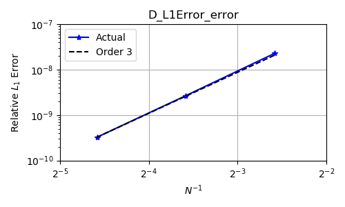
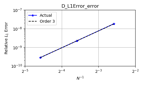
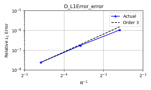
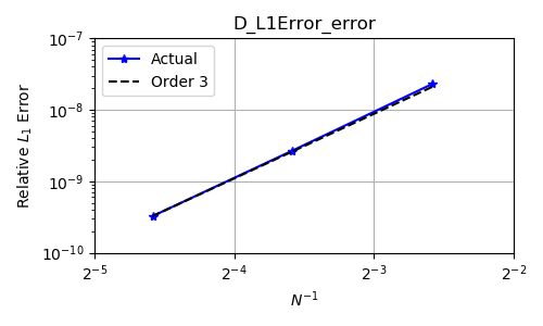
For all eigenvalue/eigenvector cases, , tests are run for the rotation configurations in Table 1 with basis order and time integrator combinations of (0, RK1), (1, SSPRK2), and (2, SSPRK3). The domain, , and number of elements in each direction, , is calculated based on the rotation matrix, :
| (82) |
| (83) |
where is the number of wavelengths, is the direction vector for the default orientation of the wave , is the refinement multiplier per refinement increment (default ), is the refinement level, and is the base number of elements, which varies for 1D, 2D, and 3D.
For these tests, the velocity was either set to or , where . The base time step is determined by running the test with adaptive time stepping, which adjusts the time step to maintain a certain CFL during the test (0.2 in this case). The test is then run again 3 times, each time increasing the refinement in both space and time by a factor of 2 to maintain a constant CFL. The L1Error and L2Error are gathered for each test and are fitted against the results using the following equation:
| (84) |
where , , and are fitting constants. The exponent is the convergence order, which is expected to be 1, 2, and 3 for the time integrators RK1, SSPRK2, and SSPRK3 respectively. Results for the 3D, non-grid-aligned, zero velocity, basis order 2, SSPRK3, test case are shown in Tab. 2, while the L1Error is plotted against the expected values for the conserved quantity in Fig. 6.
| Quantity | Eigenvalue/eigenvector Test Case | ||||
|---|---|---|---|---|---|
| - | + | ||||
| 3.099989 | 3.036570 | 2.561624 | 2.561624 | 3.099989 | |
| 3.079648 | - | 2.838988 | 2.838988 | 3.079648 | |
| 3.079648 | - | 2.879077 | 2.824568 | 3.079648 | |
| 3.079648 | - | 2.824568 | 2.879077 | 3.079648 | |
| 3.099989 | 3.036570 | 2.561652 | 2.561652 | 3.099989 | |
| 3.099989 | 3.036570 | - | - | 3.099989 | |
| 3.079655 | - | 2.838988 | 2.838988 | 3.079655 | |
| 3.079655 | - | 2.879077 | 2.824568 | 3.079655 | |
| 3.079655 | - | 2.824568 | 2.879077 | 3.079655 | |
| 3.099989 | - | - | - | 3.099989 | |
4.2 1D Riemann Problems
We now investigate the accuracy of the relativistic hydrodynamics method through considering the evolution of a set of standard 1D Riemann problems in order to characterize how well the code handles shocks. For initial conditions, we use three standard blast waves and a reflecting wall test from Martí and Müller 2003, Martí and Müller 2015 and one Sod shock tube, and a reflecting wall test for a total of five different 1D Riemann problems.
For the first four 1D Riemann problems, we use a grid with Dirichlet boundary conditions. These four tests begin divided into a primitive state on the left for and right for . In the fifth test, we replace the boundary condition at with a reflecting boundary and use a uniform initial primitive state through the domain. In all cases, we set and use the ideal equation of state with for the first four tests and for the fifth test.
For each of the five 1D Riemann problems, we use a grid with Dirichlet boundary conditions except for test 5, which uses a reflecting boundary condition on the right wall. The tests begin divided into a primitive state on the left for and right for except for test 5, which begins with a constant primitive state throughout the volume. In all cases, .
For reference data, we compute a cell solution using a HLLC Riemann solver, a second order Van-Leer integrator due to Stone et al. 2020 for each of the tested Riemann problems. We run the each 1D Riemann problem with five resolutions in powers of two from to cells with polynomial basis orders , , and using the HLLC Riemann solver and the iterative primitives recovery method for the ideal gas. For basis orders and , we use the limiter from Moe et al. 2015 in addition to the physicality-enforcing operator from § 2.5. The physicality-enforcing operator was necessary for all tests with basis orders over . Fig. 7 shows the density, longitudinal velocity, pressure, and Lorentz factor from the five 1D Riemann problems using with the three polynomial basis orders and the reference solution. Fig. 8 shows a log-log plot of the L1 error of the relativistic density, longitudinal relativistic momentum density, and total energy density compared to the reference solution along with power fits to the convergence rate and the expected rate of convergence.
1D Riemann problem 1 is a mildy relativistic blast wave with initial conditions
| (85) |
where we have followed Núñez-de la Rosa and Munz 2018 and used a pressure close to zero for the right side primitive state for numerical reasons. For this test, we use an adiabatic index . We evolve the shock until . For this first test we achieved the expected convergence rate in all variables except for the density for basis order 0, which suffers from slow converging dissipation around the blast wave. We also see a small cusp in velocity and oscillations in basis order 2 at the trailing edge of the blast wave which are more apparent in the Lorentz factor. L1 error of basis orders 1 and 2 are comparable, highlighting the difficultly in achieving high-order convergence with higher order methods when the problem contains shocks. However, since the basis order 2 test has more degrees of freedom than the basis order 1 test, the L1 error per degree of freedom is still lower for basis order 2, indicating that higher order bases can still be more efficient.
1D Riemann problem 2 is a highly relativistic blast wave with initial conditions
| (86) |
using an adiabatic index and evolved until . In this test, we see that the sharpness of the resolved density of the blast wave changes with resolution. We see it the sharpest with basis order 1, second with basis order 0, and most diffuse with basis order 2, although for each basis the sharpness improves with resolution. We see a slight cusp in the Lorentz factor for all basis orders just behind the blastwave where the velocity approaches but in the high resolution finite volume method the region has a flat Lorentz factor. The sharp blast wave in density causes problems for convergence at basis order 0 while higher order bases achieve the expected convergence.
1D Riemann problem 3 is also a highly relativistic blast wave but with a transverse velocity with initial conditions
| (87) |
with an adiabatic index and evolved until . With the addition of a relativistic transverse velocity, the blast wave widens into a square plateau in density, somewhat similar to problem 1. Like in problem 2, we find that basis order 1 best captures the blast wave, although resolution improves accuracy for all basis orders. In the Lorentz factor we see a small cusp at the rightmost edge of the rarefaction and some smearing across the blastwave. The wider blast wave allows basis order 0 to achieve the expected convergence rate. L1 error for basis order 2 is greater than the L1 error for basis order 1, although this is mostly due to more degrees of freedom in the summation of the L1 error for basis order 1.
1D Riemann problem 4 is a Sod shock with initial conditions
| (88) |
using an adiabatic index and evolving until . We see some diffusivity across the contact discontinuity and at the leftmost edge of the rarefaction.
For the fifth 1D Riemann problem we study a highly relativistic flow moving to the right and reflecting against the right wall. We use the initial conditions
| (89) |
with an adiabatic index and evolved until . We see a small cusp in the Lorentz factor at the left edge of the piled up stationary mass. For higher order bases, we see wall heating causing spurious oscillations in the reflected fluid. These leads to slow rates of convergence for basis order 2.
4.3 1D Taub-Matthews Equation of State Test
We test the Taub-Matthews approximation to the Synge equation of state against the ideal equation of state using the fifth blast wave problem from Ryu et al. 2006, which highlights the differences between the Synge gas and ideal gas. The initial conditions for the test, using the same notation and domain as §4.2, are
| (90) |
which evolves into a blast wave. In the initial state, the temperature stand-in on the left-hand side is relativistic while on the right-hand side is non-relativistic. As such, for an ideal equation of state, an adiabatic index of is appropriate for the left-hand side while is appropriate for the right-hand side. The Taub-Matthew equation of state approximation allows accurate modeling of both sides with a single equation of state.
We show results for the blast wave with the three different equation of state in Fig. 9. The Synge gas as approximated by the Taub-Matthews equation of state behaves like the relativistic ideal gas on the left side of the blast wave (which is contained within at as shown) and like the non-relativistic ideal gas on the right side. This is most evident in the velocity profiles and pressure profiles in the relativistic region that occupies most of the domain at this time. The equivalent adiabatic index of the Taub-Matthews equation of state is expectedly in the relativistic region and in the non-relativistic region, and varies between these values across the blast wave. In this region within the blast wave, the peak density with the Taub-Matthews equation of state falls between the extremes of the two ideal gases. Notably, the blast wave with the Taub-Matthew equation of state travels slightly faster than either ideal gases, and the minimum transverse velocity is also lower. These results are consistent with the blast waves evolved with the Taub-Matthews equation of state in Ryu et al. 2006.
4.4 2D Riemann Problems
Next, we test the robustness of the method evolving intersecting shocks in 2D using the three 2D Riemann problems used in Zanna and Bucciantini 2002, Núñez-de la Rosa and Munz 2018. In each of the three problems, the problem is defined with a domain divided into four quadrants with different initial states. Following Núñez-de la Rosa and Munz 2018, we denote these states using
| (91) | ||||
| (92) | ||||
| (93) | ||||
| (94) |
and denote the initial primitive states in each of these quadrants by , , , and respectively. For all of these Riemann problems, we use an adiabatic index of , use everywhere, and use transmissive boundary conditions on all sides. We evolve each Riemann problem to . For all 2D shock tests we use the Moe limiter [23] and HLLC Riemann solver.
4.4.1 2D Riemann Problems: Test 1
In this test, the domain begins with a low density and pressure region in the upper right, a high density and pressure region in the lower left, and intermediate density and high pressure regions in the upper left and lower right with initial velocities moving into the lower density region with .
| (95) | ||||
| (96) | ||||
| (97) | ||||
| (98) |

Results from the first 2D Riemannn problem is shown in Fig. 10 with the and order bases, the system evolves with stationary contact discontinuities between the high density and moving intermediate density regions, planar shocks moving from the intermediate density regions into the low density regions, and curved shocks bowing into the intermediate density regions from the diagonal. A jet-like, low density structure forms into the high density region with gentle density and pressure gradients forming ahead and behind it. Our method evolves the curved shocks with symmetric shock fronts using both low order and high-order bases. When using bases over order, the physicality-enforcing operator described in §2.5 is necessary to avoid negative densities, pressures, and otherwise unphysical states. With the order basis, we see subtle boundary effects where the shocks traveling transverse to the boundary into the first quadrant intersect with the outflow boundary conditions. Boundary effects with the order basis are seen again in § 4.4.2 and § 4.5.2.
4.4.2 2D Riemann Problems: Test 2
In this test, all four quadrants begin with different densities, equal pressures, and each move diagonally clockwise around the origin.
| (99) | ||||
| (100) | ||||
| (101) | ||||
| (102) |

Results from the second 2D Riemannn problem are shown in Fig. 11 with the and order bases, the system develops into four vortex sheets that expand from the origin. A low rest mass region forms at the center of the vortex sheets at the origin. The physicality-enforcing operator ensures positive densities and pressures in this region. With the order basis, we see subtle boundary effects where the shocks traveling transverse to the boundary into the first quadrant intersect with the outflow boundary conditions. These boundary effects are not apparent with the order basis.
4.4.3 2D Riemann Problems: Test 3
This tests begins with overdense first and third quadrants following
| (103) | ||||
| (104) | ||||
| (105) | ||||
| (106) |
Rarefactions move from the second and fourth quadrants into the first and third quadrants, producing curved shocks where the rarefactions intersect.

Results from the third 2D Riemann problem are shown in Fig. 12 with the order basis. The method evolves the curved shocks and rarefactions without issue. No boundary effects are apparent in this test.
4.5 Kelvin-Helmholtz Instability
The relativistic Kelvin-Helmholtz instability provides a useful benchmark with which to explore the performance of the scheme presented here for shear-flow type problems. Previous work, e.g. [45, 46] has revealed signficant differences in the performance of different numerical schemes for this classic fluid flow problem and subsequent work [47] has further elucidated the issues raised in prior works through the comparison of finite volume and spectral methods. Here, we compare the discontinuous-Galerkin scheme presented here with a finite volume method previously presented in the literature [39], explore both the linear and non-linear regime of the instability and examine performance metrics for the scheme.
We simulate the Kelvin-Helmholtz instability on a domain with a single interface along , specified with a smoothly varying profile using a mesh of square cells with twice as many cells in than , testing mesh sizes in powers of from to for a total of different mesh sizes. We tested using basis orders , , and , however due to memory constraints and increasing execution time, we forgo the highest resolution mesh using basis order and the two highest resolutions using basis order . We conduct separate tests using the HLLC and HLL Riemann solvers and using a shear velocity . We run a total of simulations exploring growth rates of the Kelvin-Helmholtz instability. In all these calculations, we use an ideal equation of state with adiabatic index using the iterative conserved-to-primitive solver, an initial density , an initial pressure , a perturbation amplitude , and a shearing layer thickness . We use so that the wavelength of the perturbations in is and for each test run until to verify from the growth rate that the transverse velocity perturbations have saturated past the linear growth phase.
4.5.1 Linear Growth Phase
We explore the growth of the instability by examining the spatial average
| (107) |
where is the domain and is the volume of the domain. Fig. 13 shows as a function of time in the left column for the Kelvin-Helmholtz instability simulations explored in this work, where Riemann solvers are grouped by column and basis order and reconstruction method grouped by rows. Except for the lowest resolution simulations, all simulations with the HLLC solver enter a linear growth phase by and display non-linear features by . By contrast, simulations that utilize the HLL Riemann solver, especially with the order basis, exhibit large levels of numerical diffusion and substantially reduced growth rates for all but the largest number of degrees of freedom. However, for basis order greater than zero, the HLL Riemann solver exhibits rapid convergence to a well-defined growth rate, while the reference finite volume schemes that utilize this same Riemann solver exhibit changing growth rates over this same range of degrees of freedom.
We quantify this result by measuring the growth rate, of by fitting to the measured using a least squares curve fit in log space over to . We measure the growth rate early in the linear growth phase from to before non-linear modes dominate. We perform the fit in log space so as to not favor the larger changes in at later times. The growth rate of for all simulations and methods versus the degrees of freedom is shown in Fig. 14. Here, the degrees of freedom for a given resolution and basis order is . Except for the discontinuous-Galerkin methods using the order basis, the growth rates using different methods converge to approximately the same value with higher resolutions. Generally, using higher order bases, using the HLL Riemann solver over the HLLC Riemann solver, and using the discontinuous-Galerkin method over the finite volume method lead to faster convergence of growth rate. Notably, the overall second order accurate discontinuous-Galerkin scheme (first order basis, second order time integration scheme) achieves a converged growth rate at lower numbers of degrees of freedom than a overall second order accurate finite volume scheme, using either the HLLC or HLL Riemann solver.
This result is explored in more detail in Fig. 15. The data of this figure shows the difference in growth rate between the highest resolution simulation with a certain method and the lower resolution simulations with the same methods versus the degrees of freedom. The discontinuous-Galerkin simulations with a order basis show the most effective convergence of the simulations explored here, with HLLC converging slightly faster at the highest resolutions and HLL converging faster at lower resolutions. By contrast, the overall second order accurate finite volume schemes exhibit slower convergence than this scheme, despite the equivalent order of accuracy, while the first order accurate discontinuous-Galerkin scheme exhibits similar convergence rates as the finite volume schemes when combined with the HLLC Riemann solver, but low convergence rates with the HLL solver. We also note that the discontinuous-Galerkin simulations with a order basis do not converge below a difference even with high resolutions, which we attribute to interaction of the flow with outflow boundary conditions used here, highlighting the need for improved fidelity boundary conditions in order to realize the promise of higher order discontinuous-Galerkin methods.


4.5.2 Non-linear Evolution
Fig. 16, 17, and 18 show the state of the Kelvin Helmholtz instability at using the method presented in this work and the reference finite volume scheme [39] with the 4 highest resolutions explored in this study. The different figures show results using , , and order bases or , , and order methods respectively, where a method is only available for our code. In Fig. 16 using our method with a order basis or a order method, we see significant differences between the HLL and HLLC solutions; the HLL Riemann solver struggles to grow the instability, although the structure of the perturbation resembles results with simple structures when using higher orders. Secondary instabilities appear to be nonexistent. By contrast, the HLLC Riemann solver generates secondary vortices that increasing in amplitude with higher resolutions. Looking at Fig. 17 and 18, the and order methods from this work quickly converge to simple structures. The finite volume method also converges to a similar simple structure, although it requires more resolution compared to the discontinuous-Galerkin method presented here.
Figs. 19, 20, and 21 show the state of the Kelvin Helmholtz instability at , which is well into the non-linear phase, using the method presented in this work and with the reference finite volume scheme with the 4 highest resolutions explored in this study. The different figures show results using , , and order methods respectively, where a is only available for our code. In Fig. 19 using our method with a order basis or a order method, we again see significant differences between the HLL and HLLC solutions. The HLLC solution grows faster than the HLL solution but neither resemble the structures seen with higher order bases. Using the HLLC Riemann solver, secondary vortices are apparent during the non-linear phase, which become more defined with higher resolution. Examining Figs. 20 and 21, the and order methods from this work quickly converge with higher resolution to simple structures during the non-linear phase. Results with HLL over HLLC and with a order basis over a order basis are generally smoother with fewer secondary vortices. The solution generated by the reference finite volume scheme also converges to roughly the same structures as the discontinuous-Galerkin method, although secondary instabilities are obvious along the interface between the primary vortices. Note that the mode of these secondary instabilities increased with resolution, with smaller but more numerous instabilities at higher resolutions.
Our interpretation of these results is that the secondary structures found in the finite volume method at the end of the linear growth phase serve to seed non-linear structures that are observed at late times; a result somewhat consistent with that reported by [47]. What is notable is that these structures vanish in the second order accurate (first order basis) discontinuous-Galerkin scheme presented here at lower resolution than in the finite volume scheme for the HLLC Riemann solver and are absent in the HLL Riemann solver based scheme, indicating a role played by the dissipation of the HLLC Riemann solver in the formation of these structures. In addition, the presence of these structures in the finite volume scheme utilizing the HLL solver and the clear dependency of the properties of these structures on the reconstruction method (PLM vs. PPM) is another point of contrast between discontinuous-Galerkin methods and finite volume schemes. This is strongly reminiscent of the results presented by [47], where finite volume schemes were demonstrated to exhibit similar secondary vortices at moderate resolutions (similar to these presented here), which then disappeared at higher resolutions; the higher resolution simulations being comparable to spectral methods. The absence of such secondary vortices for combinations of the discontinuous-Galerkin algorithms presented here suggest that these methods may be less susceptible to such considerations. However, we stress that this is a single application on both methods and that the performance of either method may depend on details of the set up of the instability. Over the development of the method, we also explored the analytic growth rate of perturbations given the initial conditions from Bodo et al. 2004, where we found that the growth rate of the instability generally did not match the analytically predicted growth rate, and that an initial transient outgoing wave from the initial perturbation caused significant boundary effects with the order basis. Although our discontinuous-Galerkin method provides apparently better results in this case, more development especially around boundary conditions is required.


4.6 Performance
To test the performance of the method on multiple architectures, we timed simulations of the Kelvin Helmholtz instability on CPUs and GPUs, using the perturbations described in §4.5. For both architectures, we time the performance of the code with using basis orders 0, 1, and 2 and resolutions of , , and with each basis order testing both HLLC and HLL for a total of 18 simulations for both architectures. We conduct CPU testing on 1024 cores spread across 22 dual socket nodes with Intel Xeon Platinum 8268 CPUs, comprising approximately in total. For GPU runs we use 32 NVidia Tesla V100-SXM2 GPUs spread across 8 nodes, comprising approximately in total. These computational resources were chosen to accommodate the memory needed for the largest simulation in the performance profiling suite.
We show profiling results with the HLLC and HLL Riemann solvers and with the , , and order bases in Fig. 22. The degree of freedom updates per second is computed with
| (108) |
which serves as a measure of computational efficiency. With the RK1, SSPRK2, and SSPRK3 integrators used for basis orders , , and we use , , and stages per step for the respective basis orders.
We show profiling results with the HLLC and HLL Riemann solvers and with the , , and order bases, between which we see little difference in performance. Comparing between the CPU and GPU runs, we see that the CPU performance becomes saturated at around while the GPUs have not saturated the performance, even with simulations using more than times the degrees of freedom. Simulations with more degrees of freedom would not fit within GPU memory here, indicating that our present implementation is unable to fully saturate GPU performance. Note that the theoretical peak throughput of the GPU resources using here is approximately three times the throughput for the CPU resources. Memory bandwidth resources between RAM and the registers on CPUs and HBM memory and the registers on GPUs is similarly greater on GPUs Since the CPUs and GPUs achieve roughly the same updates per second, this indicates underutilization of GPU FLOPS. i.e. our implementation is failing to meet computation or memory bounds, where the arithmetic-intensity of discontinuous-Galerkin methods lead to typically memory bound algorithms.
These performance characteristics are consistent with insufficient work within individual kernels to offset kernel launch overhead, as was the case in the K-Athena magnetohydrodynamics code presented in Grete et al. 2021 and was resolved in the Parthenon adaptive-mesh refinement framework and AthenaPK magnetohydrodynamics code presented in Grete et al. 2022. We performed an informal profiling of our method evolving the Kelvin-Helmholtz instability on a single V100 GPU using nvprof. With a timeline trace, we verified for problem sizes that occupied the entirety of the HBM memory of a single GPU that a large percentage of compute time on the GPU, , was dominated by short duration kernel calls. These kernel durations would be consumed by kernel launch overhead from within the CUDA API.
With the launch of each kernel, between the APIs, drivers, and hardware a few microseconds are spent launching the kernel on the GPU. Unless sufficient work is done within each kernel, this launch overhead will dominate runtime. For our implementation, the work done within individual kernels can be increased with more degrees of freedom. However, the GPU has insufficient memory to allow enough work to hide kernel launch overhead, hence the underutilization of the GPU. In Parthenon and AthenaPK, this kernel launch overhead was hidden by fusing together the work from multiple kernels into fewer, larger kernels[49]. Similar improvements would be needed for our implementation in order to saturate GPU performance.
5 Summary
We have presented a scheme to evolve the relativistic hydrodynamics equations using a discontinuous-Galerkin method. Within our scheme, we have developed a robust method for enforcing physicality of the conserved state via a operator. Our presentation of the method includes relativistic HLL and HLLC Riemann solvers, multiple methods for recovering the primitive variables from conserved variables with the ideal equation of state, and the Taub-Matthews approximation to the Synge equation of state, using physical units that keep factors of . We implement the method using the Kokkos performance portability library, which allows us to run CPUs and GPUs supported by Kokkos.
The novel physicality-enforcing operator in the work allows evolution of shocks with high-order basis methods. The operator strictly enforces positive density and pressure and subluminal velocities on all basis points within a cell by smoothing nonphysical points towards the physical volume average. Additionally, the method conserves volume averages of conserved variables.
In our exploration of methods to recover primitive variables from conserved variables when using an ideal equation of state, we found that the iterative method from Riccardi and Durante 2008 was faster, more robust, and more accurate than the analytical method from Ryu et al. 2006, consistent with findings from Riccardi and Durante 2008. The iterative method for ideal gases presented here recovers the primitive variables by solving a quartic as described in Eq. 58, which provides more digits of precision in simultaneously in sub-relativistic and ultra-relativistic regimes compared to solving in terms of the velocity or Lorentz factor. Additionally, the Newton-Raphson method as applied to Eq. 59 gives comparable accuracy to the analytic method in under 10 iterations, as is explored in Fig. 2. More iterations allow a more accurate recovery with the iterative method compared to the analytic method. In the case of our implementation, the iterative method is faster to compute for on CPUs and always faster on GPUs except in trivial cases.
Conversely, in our exploration of methods to recover primitives variables from conserved variables with the Taub-Mathews equation of state, the analytical method detailed in Ryu et al. 2006 was faster than the iterative method implemented in this work. With the Taub-Mathews equation of state, recovering the primitives requires solving a cubic equation, which has a much simpler analytical solution compared to the quartic equation for the ideal gas. Solving this cubic equation iteratively requires a bounded root solver, where we use Brent’s method in this work. The iterative method we implemented for the Taub-Matthews equation of state requires many more iterations to achieve acceptable accuracy than the iterative solver for the ideal gas. As such, we found the analytic method for the Taub-Matthews equation of state to outperform the iterative method in terms of time to solution and accuracy on both CPUs and GPUs.
With this method, we ran several standard test problems, including linear waves, 1D and 2D Riemann problems, and the relativistic Kelvin-Helmholtz problem. The iterative conserved-to-primitive solver facilitated more relativistic problems and the physicality-enforcing operator allowed stable evolution with higher order bases for problems with shocks. In some test problems with a shock moving transverse to an outflow boundary conditions, we saw some non-physical boundary effects when using a order basis.
In our tests of the Kelvin-Helmholtz instability, comparing to results using a finite volume reference scheme [39], the discontinuous-Galerkin method presented in this work can better suppress secondary vortices and instabilities compared to the finite volume method. Our method works best with a order basis, which is a order method in space and time, since the order basis is slow to grow the instability with low resolution while with the order basis boundary effects enter in at the outflow boundaries with high resolution.
In the tests of the Kelvin-Helmholtz instability and some of the 2D Riemann problems, we saw numerical boundary effects enter at the outflow boundary conditions, which increased with higher resolutions. Further development of the outflow boundaries with higher order bases is required.
Finally, in the exploration of the performance of our implementation evolving the Kelvin-Helmholtz instability, we found that our implementation is unable to saturate performance on GPUs before the problem size grows too large for the GPU memory. From these performance results and profiling using nvprof, we suspect that insufficient work inside individual kernels, leading to kernel launch overhead dominating runtime, is responsible for the lack of performance on GPUs. Combining the work from multiple kernels – as was done in the Parthenon framework presented in Grete et al. 2021 – would be needed for our implementation in order to saturate GPU performance.
Acknowledgments
Sandia National Laboratories is a multimission laboratory managed and operated by National Technology & Engineering Solutions of Sandia, LLC, a wholly owned subsidiary of Honeywell International Inc., for the U.S. Department of Energy’s National Nuclear Security Administration under contract DE-NA0003525. This paper describes objective technical results and analysis. Any subjective views or opinions that might be expressed in the paper do not necessarily represent the views of the U.S. Department of Energy or the United States Government. This work was supported in part by LDRD project #209240. SAND #SAND2022-3784 O
References
- Blandford et al. [2019] R. Blandford, D. Meier, A. Readhead, Relativistic Jets from Active Galactic Nuclei, Annual Review of Astronomy and Astrophysics 57 (1) (2019) 467–509, doi:10.1146/annurev-astro-081817-051948.
- Villiers et al. [2003] J.-P. D. Villiers, J. F. Hawley, J. H. Krolik, Magnetically Driven Accretion Flows in the Kerr Metric. I. Models and Overall Structure, The Astrophysical Journal 599 (2) (2003) 1238, ISSN 0004-637X, doi:10.1086/379509.
- Kumar and Zhang [2015] P. Kumar, B. Zhang, The Physics of Gamma-Ray Bursts & Relativistic Jets, Physics Reports 561 (2015) 1–109, ISSN 0370-1573, doi:10.1016/j.physrep.2014.09.008.
- Sinars et al. [2020] D. B. Sinars, M. A. Sweeney, C. S. Alexander, D. J. Ampleford, T. Ao, J. P. Apruzese, C. Aragon, D. J. Armstrong, K. N. Austin, T. J. Awe, A. D. Baczewski, J. E. Bailey, K. L. Baker, C. R. Ball, H. T. Barclay, S. Beatty, K. Beckwith, K. S. Bell, J. F. Benage, N. L. Bennett, K. Blaha, D. E. Bliss, J. J. Boerner, C. J. Bourdon, B. A. Branch, J. L. Brown, E. M. Campbell, R. B. Campbell, D. G. Chacon, G. A. Chandler, K. Chandler, P. J. Christenson, M. D. Christison, E. B. Christner, R. C. Clay, K. R. Cochrane, A. P. Colombo, B. M. Cook, C. A. Coverdale, M. E. Cuneo, J. S. Custer, A. Dasgupta, J.-P. Davis, M. P. Desjarlais, D. H. Dolan, J. D. Douglass, G. S. Dunham, S. Duwal, A. D. Edens, M. J. Edwards, E. G. Evstatiev, B. G. Farfan, J. R. Fein, E. S. Field, J. A. Fisher, T. M. Flanagan, D. G. Flicker, M. D. Furnish, B. R. Galloway, P. D. Gard, T. A. Gardiner, M. Geissel, J. L. Giuliani, M. E. Glinsky, M. R. Gomez, T. Gomez, G. P. Grim, K. D. Hahn, T. A. Haill, N. D. Hamlin, J. H. Hammer, S. B. Hansen, H. L. Hanshaw, E. C. Harding, A. J. Harvey-Thompson, D. Headley, M. C. Herrmann, M. H. Hess, C. Highstrete, O. A. Hurricane, B. T. Hutsel, C. A. Jennings, O. M. Johns, D. Johnson, M. D. Johnston, B. M. Jones, M. C. Jones, P. A. Jones, P. E. Kalita, R. J. Kamm, J. W. Kellogg, M. L. Kiefer, M. W. Kimmel, P. F. Knapp, M. D. Knudson, A. Kreft, G. R. Laity, P. W. Lake, D. C. Lamppa, W. L. Langston, J. S. Lash, K. R. LeChien, J. J. Leckbee, R. J. Leeper, G. T. Leifeste, R. W. Lemke, W. Lewis, S. A. Lewis, G. P. Loisel, Q. M. Looker, A. J. Lopez, D. J. Lucero, S. A. MacLaren, R. J. Magyar, M. A. Mangan, M. R. Martin, T. R. Mattsson, M. K. Matzen, A. J. Maurer, M. G. Mazarakis, R. D. McBride, H. S. McLean, C. A. McCoy, G. R. McKee, J. L. McKenney, A. R. Miles, J. A. Mills, M. D. Mitchell, N. W. Moore, C. E. Myers, T. Nagayama, G. Natoni, A. C. Owen, S. Patel, K. J. Peterson, T. D. Pointon, J. L. Porter, A. J. Porwitzky, S. Radovich, K. S. Raman, P. K. Rambo, W. D. Reinhart, G. K. Robertson, G. A. Rochau, S. Root, D. V. Rose, D. C. Rovang, C. L. Ruiz, D. E. Ruiz, D. Sandoval, M. E. Savage, M. E. Sceiford, M. A. Schaeuble, P. F. Schmit, M. S. Schollmeier, J. Schwarz, C. T. Seagle, A. B. Sefkow, D. B. Seidel, G. A. Shipley, J. Shores, L. Shulenburger, S. C. Simpson, S. A. Slutz, I. C. Smith, C. S. Speas, P. E. Specht, M. J. Speir, D. C. Spencer, P. T. Springer, A. M. Steiner, B. S. Stoltzfus, W. A. Stygar, J. Ward Thornhill, J. A. Torres, J. P. Townsend, C. Tyler, R. A. Vesey, P. E. Wakeland, T. J. Webb, E. A. Weinbrecht, M. R. Weis, D. R. Welch, J. L. Wise, M. Wu, D. A. Yager-Elorriaga, A. Yu, E. P. Yu, Review of Pulsed Power-Driven High Energy Density Physics Research on Z at Sandia, Physics of Plasmas 27 (7) (2020) 070501, ISSN 1070-664X, doi:10.1063/5.0007476.
- May and White [1966] M. M. May, R. H. White, Hydrodynamic Calculations of General-Relativistic Collapse, Physical Review 141 (4) (1966) 1232–1241, doi:10.1103/PhysRev.141.1232.
- Wilson [1972] J. R. Wilson, Numerical Study of Fluid Flow in a Kerr Space, The Astrophysical Journal 173 (1972) 431, ISSN 0004-637X, doi:10.1086/151434.
- Martí and Müller [2003] J. M. Martí, E. Müller, Numerical Hydrodynamics in Special Relativity, Living Reviews in Relativity 6 (1), ISSN 1433-8351, doi:10.12942/lrr-2003-7.
- Fuhry et al. [2014] M. Fuhry, A. Giuliani, L. Krivodonova, Discontinuous Galerkin Methods on Graphics Processing Units for Nonlinear Hyperbolic Conservation Laws, International Journal for Numerical Methods in Fluids 76 (12) (2014) 982–1003, ISSN 1097-0363, doi:10.1002/fld.3963.
- Mathews [1971] W. G. Mathews, The Hydromagnetic Free Expansion of a Relativistic Gas, The Astrophysical Journal 165 (1971) 147, doi:10.1086/150883.
- Synge [1957] J. Synge, The Relativistic Gas, Series in Physics, North-Holland Publishing Company, 1957.
- Edwards et al. [2014] H. C. Edwards, C. R. Trott, D. Sunderland, Kokkos: Enabling manycore performance portability through polymorphic memory access patterns, Journal of Parallel and Distributed Computing 74 (12) (2014) 3202 – 3216, ISSN 0743-7315, doi:https://doi.org/10.1016/j.jpdc.2014.07.003, URL http://www.sciencedirect.com/science/article/pii/S0743731514001257, domain-Specific Languages and High-Level Frameworks for High-Performance Computing.
- Riccardi and Durante [2008] G. Riccardi, D. Durante, Primitive Variable Recovering in Special Relativistic Hydrodynamics Allowing Ultra-Relativistic Flows, in: International Mathematical Forum, vol. 42, 2081–2111, 2008.
- Mignone and Bodo [2006] A. Mignone, G. Bodo, An HLLC Solver for Relativistic Flows – II. Magnetohydrodynamics, Monthly Notices of the Royal Astronomical Society 368 (3) (2006) 1040–1054, ISSN 0035-8711, 1365-2966, doi:10.1111/j.1365-2966.2006.10162.x.
- Schneider et al. [1993] V. Schneider, U. Katscher, D. H. Rischke, B. Waldhauser, J. A. Maruhn, C. D. Munz, New Algorithms for Ultra-relativistic Numerical Hydrodynamics, Journal of Computational Physics 105 (1) (1993) 92–107, ISSN 0021-9991, doi:10.1006/jcph.1993.1056.
- Ryu et al. [2006] D. Ryu, I. Chattopadhyay, E. Choi, Equation of State in Numerical Relativistic Hydrodynamics, The Astrophysical Journal Supplement Series 166 (1) (2006) 410–420, ISSN 0067-0049, 1538-4365, doi:10.1086/505937.
- Taub [1948] A. H. Taub, Relativistic Rankine-Hugoniot Equations, Physical Review 74 (3) (1948) 328–334, doi:10.1103/PhysRev.74.328.
- Mignone and McKinney [2007] A. Mignone, J. C. McKinney, Equation of State in Relativistic Magnetohydrodynamics: Variable versus Constant Adiabatic Index, Monthly Notices of the Royal Astronomical Society 378 (2007) 1118–1130, ISSN 0035-8711, doi:10.1111/j.1365-2966.2007.11849.x.
- Núñez-de la Rosa and Munz [2018] J. Núñez-de la Rosa, C.-D. Munz, Hybrid DG/FV Schemes for Magnetohydrodynamics and Relativistic Hydrodynamics, Computer Physics Communications 222 (2018) 113–135, ISSN 0010-4655, doi:10.1016/j.cpc.2017.09.026.
- Cockburn and Shu [1989] B. Cockburn, C.-W. Shu, TVB Runge–Kutta local projection discontinuous Galerkin finite element method for conservation laws. II. General framework, Mathematics of computation 52 (186) (1989) 411–435.
- Cockburn et al. [1989] B. Cockburn, S.-Y. Lin, C.-W. Shu, TVB Runge–Kutta local projection discontinuous Galerkin finite element method for conservation laws III: one-dimensional systems, Journal of computational Physics 84 (1) (1989) 90–113.
- Cockburn et al. [1990] B. Cockburn, S. Hou, C.-W. Shu, The Runge-Kutta local projection discontinuous Galerkin finite element method for conservation laws. IV. The multidimensional case, Mathematics of Computation 54 (190) (1990) 545–581.
- Cockburn and Shu [1998] B. Cockburn, C.-W. Shu, The Runge–Kutta discontinuous Galerkin method for conservation laws V: multidimensional systems, Journal of Computational Physics 141 (2) (1998) 199–224.
- Moe et al. [2015] S. A. Moe, J. A. Rossmanith, D. C. Seal, A Simple and Effective High-Order Shock-Capturing Limiter for Discontinuous Galerkin Methods, arXiv:1507.03024 [math] .
- van Leer [1979] B. van Leer, Towards the Ultimate Conservative Difference Scheme. V. A Second-Order Sequel to Godunov’s Method, Journal of Computational Physics 32 (1) (1979) 101–136, ISSN 0021-9991, doi:10.1016/0021-9991(79)90145-1.
- Beckwith and Stone [2011] K. Beckwith, J. M. Stone, A Second-order Godunov Method for Multi-dimensional Relativistic Magnetohydrodynamics, The Astrophysical Journal Supplement Series 193 (2011) 6, ISSN 0067-0049, doi:10.1088/0067-0049/193/1/6.
- Gottlieb et al. [2011] S. Gottlieb, D. I. Ketcheson, C.-W. Shu, Strong Stability Preserving Runge-Kutta and Multistep Time Discretizations, World Scientific, ISBN 978-981-4289-26-9, 2011.
- Gottlieb [2015] S. Gottlieb, Strong Stability Preserving Time Discretizations: A Review, in: R. M. Kirby, M. Berzins, J. S. Hesthaven (Eds.), Spectral and High Order Methods for Partial Differential Equations ICOSAHOM 2014, Lecture Notes in Computational Science and Engineering, Springer International Publishing, Cham, ISBN 978-3-319-19800-2, 17–30, doi:10.1007/978-3-319-19800-2_2, 2015.
- Ferracina and Spijker [2005] L. Ferracina, M. Spijker, An Extension and Analysis of the Shu-Osher Representation of Runge-Kutta Methods, Mathematics of Computation 74 (249) (2005) 201–219, ISSN 0025-5718, 1088-6842, doi:10.1090/S0025-5718-04-01664-3.
- Ferracina and Spijker [2004] L. Ferracina, M. N. Spijker, Stepsize Restrictions for the Total-Variation-Diminishing Property in General Runge–Kutta Methods, SIAM Journal on Numerical Analysis 42 (3) (2004) 1073–1093, ISSN 0036-1429, doi:10.1137/S0036142902415584.
- Higueras [2004] I. Higueras, On Strong Stability Preserving Time Discretization Methods, Journal of Scientific Computing 21 (2) (2004) 193–223, ISSN 1573-7691, doi:10.1023/B:JOMP.0000030075.59237.61.
- Higueras [2005] I. Higueras, Representations of Runge–Kutta Methods and Strong Stability Preserving Methods, SIAM Journal on Numerical Analysis 43 (3) (2005) 924–948, ISSN 0036-1429, doi:10.1137/S0036142903427068.
- Shu and Osher [1989] C.-W. Shu, S. Osher, Efficient Implementation of Essentially Non-Oscillatory Shock-Capturing Schemes, II, Journal of Computational Physics 83 (1) (1989) 32–78, ISSN 0021-9991, doi:10.1016/0021-9991(89)90222-2.
- Gottlieb and Shu [1998] S. Gottlieb, C.-W. Shu, Total Variation Diminishing Runge-Kutta Schemes, Mathematics of Computation 67 (221) (1998) 73–85, ISSN 0025-5718, 1088-6842, doi:10.1090/S0025-5718-98-00913-2.
- Mignone and Bodo [2005] A. Mignone, G. Bodo, An HLLC Riemann Solver for Relativistic Flows – I. Hydrodynamics, Monthly Notices of the Royal Astronomical Society 364 (1) (2005) 126–136, ISSN 0035-8711, 1365-2966, doi:10.1111/j.1365-2966.2005.09546.x.
- Wu and Tang [2016] K. Wu, H. Tang, PHYSICAL-CONSTRAINT-PRESERVING CENTRAL DISCONTINUOUS GALERKIN METHODS FOR SPECIAL RELATIVISTIC HYDRODYNAMICS WITH A GENERAL EQUATION OF STATE, The Astrophysical Journal Supplement Series 228 (1) (2016) 3, ISSN 1538-4365, doi:10.3847/1538-4365/228/1/3.
- Brent [1973] R. P. Brent, Algorithms for Minimization Without Derivatives, Prentice-Hall, Englewood Cliffs, New Jersey, ISBN 0-13-022335-2, 1973.
- Tukey [1977] J. W. Tukey, Exploratory Data Analysis, Reading, Mass. : Addison-Wesley Pub. Co., ISBN 978-0-201-07616-5, 1977.
- Stone et al. [2020] J. M. Stone, K. Tomida, C. J. White, K. G. Felker, The Athena++ Adaptive Mesh Refinement Framework: Design and Magnetohydrodynamic Solvers, The Astrophysical Journal Supplement Series 249 (1) (2020) 4, ISSN 0067-0049, doi:10.3847/1538-4365/ab929b.
- Mignone et al. [2011] A. Mignone, C. Zanni, P. Tzeferacos, B. van Straalen, P. Colella, G. Bodo, THE PLUTO CODE FOR ADAPTIVE MESH COMPUTATIONS IN ASTROPHYSICAL FLUID DYNAMICS, The Astrophysical Journal Supplement Series 198 (1) (2011) 7, ISSN 0067-0049, doi:10.1088/0067-0049/198/1/7.
- Stone et al. [2008] J. M. Stone, T. A. Gardiner, P. Teuben, J. F. Hawley, J. B. Simon, Athena: A New Code for Astrophysical MHD, The Astrophysical Journal Supplement Series 178 (1) (2008) 137–177, ISSN 0067-0049, 1538-4365, doi:10.1086/588755.
- Keppens and Meliani [2008] R. Keppens, Z. Meliani, Linear wave propagation in relativistic magnetohydrodynamics, Physics of Plasmas 15 (10) (2008) 102103, doi:10.1063/1.2991408, URL https://doi.org/10.1063/1.2991408.
- Mignone et al. [2005] A. Mignone, T. Plewa, G. Bodo, The Piecewise Parabolic Method for Multidimensional Relativistic Fluid Dynamics, The Astrophysical Journal Supplement Series 160 (1) (2005) 199, ISSN 0067-0049, doi:10.1086/430905.
- Martí and Müller [2015] J. M. Martí, E. Müller, Grid-Based Methods in Relativistic Hydrodynamics and Magnetohydrodynamics, Living Reviews in Computational Astrophysics 1 (1) (2015) 3, ISSN 2365-0524, doi:10.1007/lrca-2015-3.
- Zanna and Bucciantini [2002] L. D. Zanna, N. Bucciantini, An Efficient Shock-Capturing Central-Type Scheme for Multidimensional Relativistic Flows - I. Hydrodynamics, Astronomy & Astrophysics 390 (3) (2002) 1177–1186, ISSN 0004-6361, 1432-0746, doi:10.1051/0004-6361:20020776.
- Mignone et al. [2009] A. Mignone, M. Ugliano, G. Bodo, A five-wave Harten-Lax-van Leer Riemann solver for relativistic magnetohydrodynamics, Monthly Notices of the Royal Astronomical Society 393 (4) (2009) 1141–1156, doi:10.1111/j.1365-2966.2008.14221.x.
- Beckwith and Stone [2011] K. Beckwith, J. M. Stone, A Second-order Godunov Method for Multi-dimensional Relativistic Magnetohydrodynamics, The Astrophysical Journal Supplement Series 193 (1) 6, doi:10.1088/0067-0049/193/1/6.
- Lecoanet et al. [2016] D. Lecoanet, M. McCourt, E. Quataert, K. J. Burns, G. M. Vasil, J. S. Oishi, B. P. Brown, J. M. Stone, R. M. O’Leary, A validated non-linear Kelvin-Helmholtz benchmark for numerical hydrodynamics, Monthly Notices of the Royal Astronomical Society 455 (4) (2016) 4274–4288, doi:10.1093/mnras/stv2564.
- Bodo et al. [2004] G. Bodo, A. Mignone, R. Rosner, Kelvin-Helmholtz Instability for Relativistic Fluids, PHYSICAL REVIEW E (2004) 4.
- Grete et al. [2021] P. Grete, F. W. Glines, B. W. O’Shea, K-Athena: A Performance Portable Structured Grid Finite Volume Magnetohydrodynamics Code, IEEE Transactions on Parallel and Distributed Systems 32 (1) (2021) 85–97, ISSN 1558-2183, doi:10.1109/TPDS.2020.3010016.
- Grete et al. [2022] P. Grete, J. C. Dolence, J. M. Miller, J. Brown, B. Ryan, A. Gaspar, F. Glines, S. Swaminarayan, J. Lippuner, C. J. Solomon, G. Shipman, C. Junghans, D. Holladay, J. M. Stone, Parthenon – a Performance Portable Block-Structured Adaptive Mesh Refinement Framework, arXiv:2202.12309 [astro-ph] .