From Noncommutative Geometry to Random Matrix TheoryEmail addresses: hhessam@uwo.ca, masoud@uwo.ca, npagliar@uwo.ca, lverhoe@uwo.ca

Spectral triples were introduced by Connes in [26] (see also [30]) and are defined by data $(\mathcal{A},\mathcal{H},D)$ where $\mathcal{A}$ is a unital, involutive, complex, associative algebra acting by bounded operators on a complex Hilbert space $\mathcal{H}$, and $D$ is a self-adjoint (in general unbounded) operator acting on $\mathcal{H}.$ This data is further required to satisfy certain finiteness and regularity conditions, which are automatically satisfied if $\mathcal{A}$ and $\mathcal{H}$ are finite dimensional. Since this will always be the case in this survey we omit these conditions here.

A real spectral triple is a spectral triple equipped with two additional operators $J$ and $\gamma$ called the charge conjugation and the chirality operator, where $J:\mathcal{H}\to\mathcal{H}$ is an anti-linear real structure, with the requirement that $[a,JbJ^{-1}]=0$ for all $a,b\in\mathcal{A}$, and $\gamma:\mathcal{H}\to\mathcal{H}$ is a self-adjoint operator with $\gamma^{2}=1$. The data $(\mathcal{A},\mathcal{H},D,J,\gamma)$ is required to satisfy some further compatibility conditions between $D$, $J$, $\gamma$, and the representation of $\mathcal{A}$ which we will recall in Definition 1.1.

The overall idea is that a real spectral triple is a noncommutative analogue of a $\text{spin}^{c}$ Riemannian manifold and its canonical Dirac operator. In fact, any closed $\text{spin}^{c}$ Riemannian manifold $M$ defines a real (commutative) spectral triple as follows. The algebra $\mathcal{A}=C^{\infty}(M)$ is the algebra of smooth complex valued functions on $M$. The Hilbert space consists of square integrable sections of the spinor bundle, with $\mathcal{A}$ acting as multiplication operators. The operator $D$ is the Dirac operator of $M$ acting on the spinors, and $J$ and $\gamma$ are the standard charge conjugation and chirality operators. The reconstruction theorem of Connnes states that, conversely, a commutative real spectral triple, i.e. a triple where $\mathcal{A}$ is commutative, satisfying some natural conditions is the spectral triple of a $\text{spin}^{c}$ Riemannian manifold [28]. The reader can find further details and many interesting commutative and non-commutative examples of spectral triples in the book of Connes and Marcolli [30], as well as their applications to the standard model of elementary particles and quantum field theory in general.

A spectral triple is called finite if both $\mathcal{A}$ and $\mathcal{H}$ are finite dimensional vector spaces. In this paper we shall primarily consider a subclass of finite real spectral triples called fuzzy spectral triples or fuzzy geometries introduced and classified in their present form by Barrett in [4]. These should be thought of as $\text{spin}^{c}$ Riemannian manifolds with a finite resolution or Plank length. It should be noted that important examples of fuzzy spectral triples like the fuzzy sphere [65, 32, 47, 4, 64] and fuzzy tori [61, 79, 7, 62] were defined and studied for their own interest before the concept of fuzzy geometry was coined. We should also mention that finite dimensional real spectral triples have been fully classified by Krajewski in [60]. Further references include [30, 66, 4, 84].

We will now specialize further to the class of fuzzy spectral triples. Let ${{\mathrm{C\ell}}_{p,q}}$, for non-negative integers $p$ and $q$, denote the real Clifford algebra associated to the vector space ${\mathbb{R}^{n}}$, $n=p+q$, and the pseudo-Euclidean metric ${\eta}$ of signature ${(p,q)}$ given by

$${\eta}(v,v)={{v_{1}}^{2}}+\cdots+{{v_{p}}^{2}}-{{v_{p+1}}^{2}}-\cdots-{{v_{p+q}}^{2}}\,,\quad v\in\mathbb{R}^{n}\,.$$

Let ${{\mathbb{C}\ell}_{n}\coloneqq{\mathrm{C\ell}}_{p,q}{\otimes_{\mathbb{R}}}\mathbb{C}\,}$ denote the complexification of ${{\mathrm{C\ell}}_{p,q}}$. Let ${{\{e_{i}\}}_{i=1}^{n}}$ denote the standard basis of ${\mathbb{R}^{n}}$. The chirality element $\Gamma\in{{\mathbb{C}\ell}_{n}}$ is defined by

$$\Gamma=\mathrm{i}^{\frac{1}{2}s(s+1)}\,e_{1}e_{2}\cdots e_{n}\,,$$

where ${s\equiv q-p\pmod{8}}$ is known as the $KO$-dimension. We denote by ${V_{p,q}}$ the unique (up to unitary equivalence) hermitian irreducible ${{\mathrm{C\ell}}_{p,q}\,}$-module, where for $n=p+q$ odd the chirality element $\Gamma$ acts trivially on $V_{p,q}\,$. The module $V_{p,q}$ also comes with a charge conjugation operator ${C:V_{p,q}\to V_{p,q}}$ (see [66, 4] for details).

The main benefit of considering fuzzy spectral triples is that their Dirac operators can be expressed in terms of the gamma matrices ${\gamma^{i}\,}$ (the image of $e_{i}$ in the Clifford algebra), and commutators or anti-commutators with Hermitian or skew-Hermitian matrices. More precisely, Barrett proved in [4] that the Dirac operator of a fuzzy spectral triple is always of the form

$$D=\sum\gamma^{I}\otimes\{K_{I},\cdot\}_{e_{I}}$$

(1)

where the sum is over increasingly ordered multi-indices $I$. If $\gamma^{I}$ is Hermitian, $e_{I}=1$ and $\{K_{I},\cdot\}_{e_{I}}=\{H_{I},\cdot\}$, where $H_{I}$ is some Hermitian matrix. If $\gamma^{I}$ is skew-Hermitian, $e_{I}=-1$ and $\{K_{I},\cdot\}_{e_{I}}=[L_{I},\cdot]$, where $L_{I}\,$is some skew-Hermitian matrix. This allows us to effectively parametrize the space of Dirac operators by matrices.

One prominent example of a fuzzy spectral triple is the fuzzy sphere [82, 85, 65, 47, 32]. Let $J_{1},J_{2},J_{3}$ be the standard skew-Hermitian generators of $\mathfrak{su}_{2}$ and denote the $2j+1$-dimensional irreducible representation of $\mathfrak{su}_{2}$ by $(\pi_{j},V_{j})$. An initial definition of a Dirac operator for the fuzzy sphere is then defined on $\mathbb{C}^{2}\otimes M_{2j+1}(\mathbb{C})\cong\mathbb{C}^{2}\otimes V_{j}\otimes V_{j}^{*}$ by

$$d=1\otimes 1+\gamma^{\mu}\otimes\left[\pi_{j}(J_{\mu}),\cdot\right]$$

with $\gamma^{\mu}=i\sigma^{\mu}$ for the Pauli matrices $\sigma^{\mu}$. This definition has two problems, it is of signature $(0,3)$ which has $KO$-dimension 3 rather than the desired 2, and it does not admit a grading [32]. Hence $d$ cannot be the Dirac operator for a fuzzy geometry. Instead we form a Dirac operator of signature $(1,3)$, by $D=\sigma^{1}\otimes d$ which admits a grading $\sigma^{3}\otimes 1$. The real structure is given by $J(v\otimes a)=\sigma_{2}\overline{v}\otimes a^{*}$.

By a Dirac ensemble we mean a statistical ensemble of fuzzy spectral triples $(\mathcal{A},\mathcal{H},D,J,\gamma)$ where the “Fermion space” $(\mathcal{A},\mathcal{H},J,\gamma)$, is kept fixed but the Dirac operator $D$ is a random variable with a given probability density. This a non-commutative analogue to a probability distribution on the space of metrics on a given manifold, as the Dirac operator encodes the metric structure while the algebra encodes the topology.

More precisely, let $\mathcal{D}$ denote the set of all possible Dirac operators $D:\mathcal{H}\rightarrow\mathcal{H}$ such that the quintuple $(\mathcal{A},\mathcal{H},D,J,\gamma)$ satisfies the conditions a), b), c), and d) of definition 1.1. Clearly $\mathcal{D}\subset\text{End}(\mathcal{H})$ is a real subspace, hence it is equipped with an inner product and thus a natural Lebesgue measure which we denote by $dD$. Given a choice of action functional $S:\mathcal{D}\to\mathbb{R}$, usually a polynomial whose choice is part of the data for a Dirac ensemble, the probability density on $\mathcal{D}$ is defined by

$$\frac{1}{Z}e^{-\tr S(D)}dD$$

where

$$Z=\int_{\mathcal{D}}e^{-\tr S(D)}dD$$

is the partition function of the model.

For fuzzy spectral triples the space of Dirac operators can be paramatrized by a combination of (skew)-Hermitian matrices or, by writing the skew-Hermitian matrices as $\mathrm{i}$ multiplied by a Hermitian one, purely by Hermitian matrices using equation (1). The probability density, and thus partition function, may then be written as a matrix integral of the form

$$Z=\int_{\mathcal{D}}e^{-\tr S(D)}dD=\int_{\mathcal{H}_{N}^{m}}e^{-\tilde{S}(H_{1},H_{2},...,H_{m})}dH_{1}...dH_{m},$$

(2)

where $\mathcal{H}_{N}$ is the space of Hermitian $N$ by $N$ matrices. For a given Dirac ensemble defined by $e^{-\tr S(D)}dD$, we refer to the third term in equation (2) as the associated random matrix ensemble. We will see this correspondence in detail in Sections 1.3 and 1.4.

The matrix ensembles associated to Dirac ensembles are usually both multi-trace or multi-matrix. Since most of the results in random matrix theory are for single matrix and single trace models, this hints that the analytic study of Dirac ensembles as matrix integrals is quite difficult in general.

For fuzzy spectral triples of dimension $n=1$ the only possible signatures are $(1,0)$ and $(0,1)$. In both case $\mathcal{H}=M_{N}(\mathbb{C})$ and the two possible choices for $D$ are as follows [4, 5]:

Type (1, 0)

The Dirac operator is the anticommutator with a Hermitian matrix $H$,

$$D=\{H,\cdot\}.$$

The trace of powers of $D$ can be computed by

$$\text{Tr}\,D^{\ell}=\sum_{k=0}^{\ell}{\ell\choose k}\tr H^{\ell-k}\tr H^{k}.$$

Type (0, 1)

The Dirac operator is the commutator with a skew-Hermitian matrix $L$,

$$D=i[L,\cdot].$$

The trace of powers of $D$ can be computed by

$$\text{Tr}\,D^{\ell}=\sum_{k=0}^{\ell}{\ell\choose k}(-1)^{k}\tr L^{\ell-k}\tr L^{k}.$$

For the action functional we can consider a quartic potential

$$Z=\int_{\mathcal{D}}e^{-g\tr D^{2}-\tr D^{4}}dD,$$

where the real parameter $g$ is called a coupling constant. In type $(1,0)$ the integral is over the space $\mathcal{H}_{N}$ of Hermitian $N\times N$ matrices and the partition function in terms of $H$ is

$$Z=\int_{\mathcal{D}}e^{-g\tr D^{2}-\tr D^{4}}dD=\int_{\mathcal{H}_{N}}e^{-2N(g\tr H^{2}+\tr H^{4})-2g(\tr H)^{2}-8\,\tr H\tr H^{3}-6(\tr H^{2})^{2}}dH.$$

The substitution of $\mathcal{H}_{N}$ for $\mathcal{D}$ is justified as the parametrization of Dirac operators by the Hermitian matrix $H$ is bijective.

In type $(0,1)$ the integral is over the space $\mathcal{L}_{N}$ of skew-Hermitian $N\times N$ matrices, and the partition function is given by

$\displaystyle Z=\int_{\mathcal{D}}e^{-g\tr D^{2}-\tr D^{4}}dD=\int_{\mathcal{L}_{N}}e^{-2g(N\tr L^{2}-(\tr L)^{2})-\left(2N\tr L^{4}-8\tr L\tr L^{3}+6(\tr L^{2})^{2}\right)}dL.$

Note that the kernel of the map $\mathcal{L}_{N}\to\mathcal{D}$ consists of the scalar matrices, which has lebesgue measure zero, justifying the substituion. We can write $L=iH$, for a Hermitian matrix $H$, to get

$\displaystyle Z=\int_{\mathcal{D}}e^{-g\tr D^{2}-\tr D^{4}}dD=i\int_{\mathcal{H}_{N}}e^{2g(N\tr H^{2}-(\tr H)^{2})+\left(-2N\tr H^{4}+8\tr H\tr H^{3}-6(\tr H^{2})^{2}\right)}dH.$

In [56] it was shown that the two terms $(\tr H)^{2}$ and $(\tr H)\tr H^{3}$ contribute nothing in the large $N$ limit, giving us the same matrix integral as the above quartic type $(1,0)$ up to a factor of $i$. This idea extends to all type $(1,0)$ and $(0,1)$ Dirac ensembles with even potentials, that is, all such ensembles will have identical real eigenvalue density in the large $N$ limit.

If one considers formal Dirac ensembles of types $(1,0)$ or $(0,1)$, it can be shown [3] that their partition functions and moments are the generating functions that count combinatorial objects know as stuffed maps in the sense of the work Borot and Shadrin in [14, 15]. Similar to the more common types of maps that arise in Hermitian matrix ensembles, the matrix integrals that generate stuffed maps obey a generalized form of Topological Recursion, called Blobbed Topological Recursion. Given the genus zero one-point and two-point generating functions one can recursively compute all higher order corrections. In particular, this (blobbed) topological recursion applies to $(1,0)$ or $(0,1)$ Dirac ensembles with multi-tracial potentials and was studied in [3].

For two dimensional fuzzy geometries there are three options. In this case the Hilbert space $\mathcal{H}=\mathbb{C}^{2}\otimes M_{N}(\mathbb{C})$, where for $p+q=2$, $\mathbb{C}^{2}\cong V_{p,q}$ is the space of spinors. The structure of the Dirac operator depends on the type as follows:

Type (2, 0)

Let

$$\gamma^{1}=\begin{pmatrix}1&0\\ 0&-1\end{pmatrix},\quad\quad\gamma^{2}=\begin{pmatrix}0&1\\ 1&0\end{pmatrix}.$$

Then,

$$D=\gamma^{1}\otimes\{H_{1},\cdot\}+\gamma^{2}\otimes\{H_{2},\cdot\},$$

where $H_{1}$ and $H_{2}$ are Hermitian matrices.

Type (1, 1)

Let

$$\gamma^{1}=\begin{pmatrix}1&0\\ 0&-1\end{pmatrix},\quad\quad\gamma^{2}=\begin{pmatrix}0&1\\ -1&0\end{pmatrix}.$$

Then,

$$D=\gamma^{1}\otimes\{H,\cdot\}+\gamma^{2}\otimes[L,\cdot],$$

where $H$ is Hermitian and $L$ is skew-Hermitian.

Type (0, 2)

Let

$$\gamma^{1}=\begin{pmatrix}i&0\\ 0&-i\end{pmatrix},\quad\quad\gamma^{2}=\begin{pmatrix}0&1\\ -1&0\end{pmatrix}.$$

Then,

$$D=\gamma^{1}\otimes[L_{1},\cdot]+\gamma^{2}\otimes[L_{2},\cdot],$$

where $L_{1},L_{2}$ are both skew-Hermitian.

The general structure of trace powers of Dirac operators ensembles of signature above 1 becomes quite complicated and has no obvious patterns. They were first studied in [70].

The associated matrix models also rise in complexity, take for example a type $(2,0)$ quartic potential

	$\displaystyle Z$	$\displaystyle=\int_{\mathcal{D}}e^{-\frac{t_{2}}{8}\tr D^{2}-\frac{t_{4}}{16}\tr D^{4}}dD$
		$\displaystyle=\int_{\mathcal{H}_{N}^{2}}e^{\tilde{S}(H_{1},H_{2})}dH_{1}dH_{2},$

where

$\displaystyle\begin{split}\tilde{S}(H_{1},H_{2})&=-t_{2}(N\tr H_{1}^{2}+N\tr H_{2}^{2})-t_{4}\left(\frac{1}{4}N\tr H_{1}^{4}+\frac{1}{4}N\tr H_{2}^{4}+N\tr H_{1}^{2}H_{2}^{2}\right.\\ &\left.-\frac{1}{2}N\tr H_{1}H_{2}H_{1}H_{2}+\frac{3}{4}(\tr H_{1}^{2})^{2}+\frac{3}{4}(\tr H_{2}^{2})^{2}+\frac{1}{2}\tr H_{1}^{2}\tr H_{2}^{2}\right)\end{split}$

(3)

are the contributing terms in the large $N$ limit. This ensemble is a bi-tracial two-matrix model. There are no known applicable analytic techniques from random matrix theory.

Note that similarly to the type $(0,1)$ geometry, Dirac ensembles with skew-Hermitian matrices can always be converted to ensembles of Hermitian matrices. So, in particular, studying models from the above geometries amounts to solving Hermitian two-matrix models.

Dirac ensembles as defined so far describe only the metric structure of a fuzzy space. The space $V_{p,q}$ plays the role of a spinor space and $M_{N}(\mathbb{C})$ plays the role of $L^{2}$-functions on the manifold so that together they make a (trivial) spinor bundle. In order to include a gauge sector we can consider Yang-Mills-Higgs fuzzy spaces [72]. This approach is based on gauge theory on almost commutative manifolds [22, 23] (see also chapter 8 of [84]), and consists of introducing a finite spectral triple playing the role of an additional (trivial) vector bundle which will carry an analogue of a connection.

Concretely, let $M_{f}=(M_{N}(\mathbb{C}),\mathcal{H}_{N},D_{f},J,\gamma)$ be a fuzzy spectral triple in the sense of Definition 1.1 and let $F=(\mathcal{A}_{F},\mathcal{H}_{F},D_{F},J_{F},\gamma_{F})$ be a finite spectral triple. This second spectral triple will be referred to as the gauge or finite spectral triple. If $\mathcal{A}_{F}=M_{n}(\mathbb{C})$ and $\mathcal{H}_{F}=M_{n}(\mathbb{C})$ the gauge triple is referred to as a Yang-Mills triple. The Gauge-Higgs fuzzy space, or Yang-Mills-Higgs fuzzy space if the gauge triple is of Yang-Mills type, is then the product spectral triple $M_{f}\times F$ given by

$$\left(M_{N}(\mathbb{C})\otimes\mathcal{A}_{F},\mathcal{H}_{N}\otimes\mathcal{H}_{F},D_{f}\otimes 1+\gamma\otimes D_{F},J\otimes J_{F},\gamma\otimes\gamma_{F}\right).$$

In this picture $D_{F}$ is usually considered fixed and controls physical aspects of the gauge fields, while $D_{f}$ will vary and describe the metric structure of the fuzzy space $M_{f}$. The smooth limit of the fuzzy Yang-Mills-Higgs triple is given by $N\to\infty$, while the size of the gauge sector $n$ remains fixed. As in Equation 1 we can write $D_{f}=\sum\gamma^{I}\otimes\{K_{I},\cdot\}_{e_{I}}$, the amplification $D_{f}\otimes 1$ can then be written as $\sum\gamma^{I}\otimes\{K_{I}\otimes 1_{n},\cdot\}_{e_{I}}$ acting on $V_{p,q}\otimes M_{N}(\mathbb{C})\otimes M_{n}(\mathbb{C})$.

The gauge theory enters this framework in the guise of inner fluctuations. These inner fluctuations [27] (see also chapter 6 of [84]) arise from Morita self-equivalences and are parametrised by the self-adjoint Connes one-forms, for a spectral triple $(\mathcal{A},\mathcal{H},D,J,\gamma)$ these one-forms are given by

$$\Omega^{1}_{D}(A)=\left\{\sum a_{i}[D,b_{i}]\,\middle|\,a_{i},b_{i}\in A\right\}\subset\End(\mathcal{H})$$

where the sum is finite. For a self-adjoint $\omega\in\Omega^{1}_{D}(A)$, the fluctuated Dirac operator is given by $D_{\omega}=D+\omega+J\omega J^{-1}$.

For the fuzzy Yang-Mills-Higgs triple we can split the fluctuations into a fuzzy and a finite part, by $a[D,b]=a[D_{f}\otimes 1,b]+a[\gamma\otimes D_{F},b]$ for $a,b\in M_{N}(\mathbb{C})\otimes M_{n}(\mathbb{C})$. The fuzzy part of this, $a[D_{f}\otimes 1,b]$, can be parametrized by $\Omega^{1}_{D_{f}}(M_{N}(\mathbb{C}))\otimes M_{n}(\mathbb{C})$, while the finite part can, independently, be parametrized by $M_{N}(\mathbb{C})\otimes\Omega^{1}_{D_{F}}(M_{n}(\mathbb{C}))$. The effect of the fuzzy part of the fluctuation, for $s\neq 1,5$, on $D_{f}\otimes 1$ is to replace $K_{I}\otimes 1_{n}$ by $K_{I}\otimes 1_{n}+T_{I}$, with $T_{I}\in\Omega^{1}_{K_{I}}(M_{N}(\mathbb{C}))\otimes M_{n}(\mathbb{C})$ of the appropriate (skew-)adjointness. The finite part of the fluctuation does not affect the fuzzy section, since it carries the action of $\gamma$ on the $V_{p,q}$ factor of $\mathcal{H}_{N}$. Instead, the finite part of the fluctuation together with $D_{F}$ itself is gathered into one term $\Phi=1_{N}\otimes D_{F}+\{\phi,\cdot\}_{\epsilon^{\prime\prime}}$ where $\epsilon^{\prime\prime}$ depends on $s$ and $\phi\in M_{N}(\mathbb{C})\otimes\Omega^{1}_{D_{F}}(M_{n}(\mathbb{C}))$. $\Phi$ is suggestively called the Higgs potential.

To motivate the term Yang-Mills-Higgs spectral triple we will specialize to the 4-dimensional Riemannian case which has signature $(p,q)=(0,4)$. In this case the fuzzy Dirac operator can be written

$$D_{f}=\sum_{\mu}\gamma^{\mu}\otimes[L_{\mu},\cdot]+\gamma^{\hat{\mu}}\otimes\{X_{\mu},\cdot\}.$$

Here $\gamma^{\hat{\mu}}$ is the increasingly ordered product of the gamma matrices for $V_{0,4}$ except $\gamma^{\mu}$. The $(0,4)$ fuzzy Dirac operator shows remarkable similarity to the Dirac operator on a commutative manifold, with $[L_{\mu},\cdot]$ taking the place of $\partial_{\mu}$ and $\{X_{\mu},\cdot\}$ taking the place of, appropriately symmetrized, Christoffel symbols. This leads us to say the fuzzy space is flat if all $X_{\mu}$ vanish.

The term Yang-Mills is further motivated by considering the gauge group [27, 30, 84] associated to a spectral triple $(A,H,D,J,\gamma)$,

$$G(A,J)=\{uJuJ^{-1}\,|\,u\in U(A)\}.$$

For a Yang-Mills fuzzy geometry, this gauge group is $PU(N)\times PU(n)$ acting in the adjoint representations on $M_{N}(\mathbb{C})\otimes M_{n}(\mathbb{C})$. The $PU(N)$ factor corresponds to symmetries of the base fuzzy geometry, while $PU(n)$ acts on the finite “vector bundle” part as a Yang-Mills gauge group.

When basing a Yang-Mills-Higgs fuzzy geometry on such a flat $(0,4)$ fuzzy space the self-adjoint one-forms, and thus the inner fluctuations, can be parametrized as $\sum_{\mu}\gamma^{\mu}\otimes A_{\mu}$ with $A_{\mu}\in\Omega^{1}_{L_{\mu}}(M_{N}(\mathbb{C}))\otimes M_{n}(\mathbb{C})$ skew-adjoint. The effect of such a fluctuation on $D_{f}$ is by replacing $L_{\mu}$ by $L_{\mu}+A_{\mu}$, making the action of inner fluctuations analogous to having a connection on the “vectorbundle” $F$. In this setting we define the field strength of a Dirac operator by $F_{\mu\nu}=\left[[L_{\mu}+A_{\mu},\cdot],[L_{\nu}+A_{\nu},\cdot]\right]$, mimicking the regular commutative definition of the field strength of a connection.

Considering the quartic potential $S(D)=g\tr D^{2}+\tr D^{4}$ we have [72], for a fluctuated $(0,4)$ Dirac operator,

$$S(D)=-2\tr F_{\mu\nu}F^{\mu\nu}+4\tr(g\theta+\theta^{2})+4\tr(g\Phi^{2}+\Phi^{4})-8\tr([L_{\mu}+A_{\mu},\Phi][L^{\mu}+A^{\mu},\Phi])$$

where $\theta=\eta^{\mu\nu}[L_{\mu}+A_{\mu},\cdot]\circ[L_{\nu}+A_{\nu},\cdot]$. Here $\theta$ is analogous to a Laplace operator and the trace is taken as operator on $M_{N}(\mathbb{C})\otimes M_{n}(\mathbb{C})$. Each of these four tracial terms has an interpretation in terms of commutative Yang-Mills-Higgs theory:

• •

  $\tr F_{\mu\nu}F^{\mu\nu}$ is analogous to the classical Yang-Mills action,

• •

  $\tr g\theta+\theta^{2}$ contains geometric information similar to a Laplace operator through a type of heat-kernel expansion [6],

• •

  $\tr g\Phi^{2}+\Phi^{4}$ represents, for appropriate values of $g$, the Higgs potential,

• •

  $\tr([L_{\mu}+A_{\mu},\Phi][L^{\mu}+A^{\mu},\Phi])$ is the coupling between the Yang-Mills connection and the Higgs field.

Hence we can include a Yang-Mills-Higgs action in a Dirac ensemble by taking the product with a finite spectral triple and considering inner fluctuations. The resulting Dirac ensemble has a space of Dirac operators $\mathcal{D}$ parametrized by, in the flat signature $(0,4)$ case, the four skew-adjoint matrices $L_{\mu}$ as well as the inner fluctuations $A_{\mu}\in\Omega^{1}_{L_{\mu}}(M_{N}(\mathbb{C}))$ and $\phi\in M_{N}(\mathbb{C})\otimes\Omega^{1}_{D_{F}}(M_{n}(\mathbb{C}))$. The physical $D_{F}$ is considered fixed. It should be noted that the $A_{\mu}$ are not necessarily independent, as they originate from a single one-form $\omega\in\Omega^{1}_{D_{f}}(M_{N}(\mathbb{C}))$ further complicating any analytical investigation of these models.

Investigating Yang-Mills-Higgs ensembles numerically or for a lower dimensional fuzzy spectral triple would be very interesting. Another open direction is the addition of a fermionic term to the action in the Dirac ensemble of the form $\langle D\psi,\psi\rangle$ where $\psi\in\mathcal{H}_{N}\otimes\mathcal{H}_{F}$ plays the role of a fermion field and would be assigned a probability distribution together with the metric and gauge fields represented by $D$ and its inner fluctuations.

The Dirac ensembles of type $(1,0)$ and $(0,1)$ discussed in Sections 1.3 can be analyzed as bi-tracial matrix models using various standard random matrix techniques that are applicable to that setting. Consider a type $(1,0)$ or $(0,1)$ Dirac ensemble with a partition function of the form

$$Z=\int_{\mathcal{D}}e^{-\frac{t_{2}}{4}\tr D^{2}+\sum_{j=3}^{d}\frac{t_{2j}}{4j}\tr D^{2j}}dD.$$

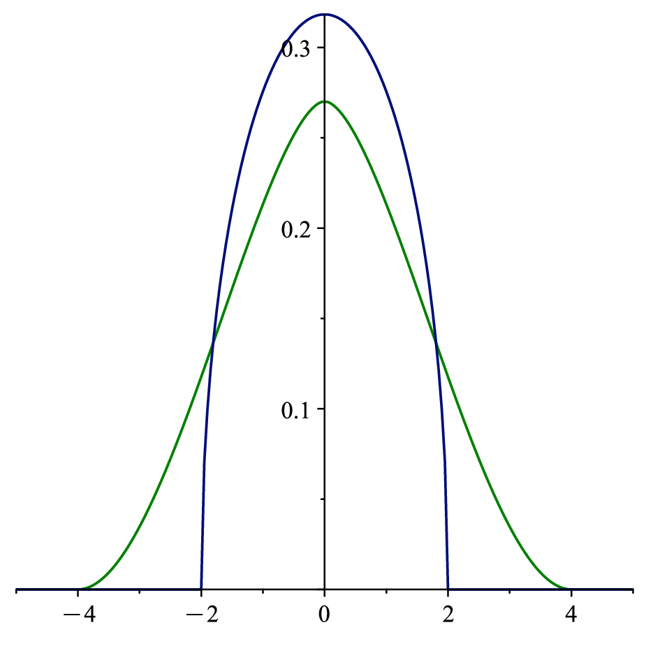
The spectra of $H$ and $L$ appearing in the associated matrix model can be computed, as we will see in subsequent sections. However, we are not just interested in the spectrum of $H$ and $L$ but also in the spectrum of $D$. It was first conjectured in [4] and later proven in [57] that if the limiting eigenvalue distribution, $\rho(x)$, of the associated random matrix ensemble exists then the limiting eigenvalue density function of $D$, $\rho_{D}$(x), is given by the integral convolution of the random matrix spectral density function with itself i.e.

$$\rho_{D}(x)=\int_{\mathbb{R}}\rho(x-t)\rho(t)dt.$$

The relationship between spectral densities is far from clear for higher signature Dirac ensembles, even for the two dimensional ones from Section 1.4. Moreover, the associated matrix models of these Dirac ensembles are multi-trace and multi-matrix, of which little is known [37].

In the large $N$ limit, there is a universality to the spectral density function of Dirac ensembles for any signature when the potential is Gaussian. In [4] a Gaussian potential

$$S(D)=\tr D^{2},$$

is investigated. When looking at the $(1,0)$ Dirac ensemble, the associated matrix potential becomes $2N\tr H^{2}+2\tr H\tr H$, where $H$ is a Hermitian matrix. For the $(0,1)$ Dirac ensemble, this potential becomes $2N\tr L^{2}+2\tr L\tr L$ where $L$ is skew-Hermitian. For these ensembles the numerics show that the distribution of the eigenvalues of $H$ and $L$ resembles Wigner’s semicircular distribution as $N$ increases. This suggests that the multi-trace term has little to no impact as $N$ gets larger. Dirac ensembles of signatures $(2,0)$, $(1,1)$ and $(0,2)$ were also studied for small matrix size, where some of the above-mentioned results also apply. Furthermore, the eigenvalue density function of the Dirac operator was conjectured to be the integral convolution of Wigner’s semicircular law with itself.

This was then proven in [57]. It was shown that in the large $N$ limit the eigenvalue density function for $D$ is universal, in the sense that for any signature $(p,q)$ the limit is the same given the right scaling. Consider the partition function of the form

$$Z=\int_{\mathcal{D}}e^{-\frac{1}{2k}\tr D^{2}}dD$$

where $k$ is the dimension of $V_{p,q}$. Then the density function of $D$, for any signature $(p,q)$, is in the large $N$ limit given by

$$\rho_{D}(x)=\int_{\mathbb{R}}\rho_{W}(x-t)\rho_{W}(t)dt,$$

where

$$\rho_{W}(x)=\frac{1}{2\pi}\sqrt{4-x^{2}}_{[-2,2]}$$

is Wigner’s Semicircular Distribution [57].

In this subsection we will discuss results related to spectral phase transitions, which we define as a configuration of coupling constants where the number of connected components of the support of the large $N$ eigenvalue density function of the random matrix ensemble changes. Like their random matrix model cousins, Dirac ensembles also exhibit phase transitions. This was first investigated numerically using Markov chain Monte Carlo methods in [5] and then in [44]. It was later proven rigorously in [56] that spectral phase transitions indeed occur in quartic type $(1,0)$ and $(0,1)$ Dirac ensembles. In this subsection we recall this quartic phase transition from [56] and we also present a new result proving a phase transition for a sextic Dirac ensemble. It is an interesting problem to analytically investigate phase transitions for Dirac ensembles of any type $(p,q)$ and a potential of any order. We believe that these phase transitions do indeed exist, but we don’t have a proof at hand. The existing results use what is known as the Coulomb gas method, the rigorous foundations of which are fully developed in [34]. We give a brief summary of this technique in Appendix A.

For Gaussian potentials, unsurprisingly, no phase transition exists. This motivated the study of a Landau-Ginzburg type quartic potential as studied in [5]. This potential is of the form

$$S(D)=g_{2}\tr D^{2}+\tr D^{4},$$

and was studied numerically for different small signatures $(p,q)$ for a matrix size of ten in [5]. It was discovered that, for many signatures, the spectrum of the Dirac operator displayed a single-cut distribution for certain values of $g_{2}$ which transitioned into a double-cut regime for different $g_{2}$. This suggests the existence of a spectral phase transition. Furthermore, it was noted that near the phase transition the spectrum of $D$ asymptotically behaves like the Dirac operator on a two dimensional manifold i.e. $\rho_{D}(\lambda)\sim C_{D}|\lambda|$, as $\lambda$ goes to infinity, where $C_{D}$ is a constant.

Computing these eigenvalue density functions explicitly even in the large $N$ limit is very difficult. Dirac ensembles of dimension higher than one with a potential more complicated than the Gaussian are multi-trace multi-matrix models about which little is known. Usual methods such as orthogonal polynomials cannot be applied because of the multi-trace terms, Weyl’s integration formula cannot be applied because of the lack of unitary invariance, and the loop equations are too complicated for Topological Recursion. Furthermore, it is not of the form of a Harish-Chandra integral, and is too complicated for a characteristic expansion. For a review of these techniques see [40].

However, for Dirac ensembles of signature $(1,0)$ or $(0,1)$, several options are available. The multi-trace terms still prevents the use of orthogonal polynomials, but the Coulomb gas technique can be applied. This was done in [56] where the type $(1,0)$ quartic model

$$Z=\int_{\mathcal{D}}e^{-g\tr D^{2}-\tr D^{4}}dD=\int_{\mathcal{H}_{N}}e^{-2N(g\tr H^{2}+\tr H^{4})-2g(\tr H)^{2}-8\,\tr H\tr H^{3}-6(\tr H^{2})^{2}}dH$$

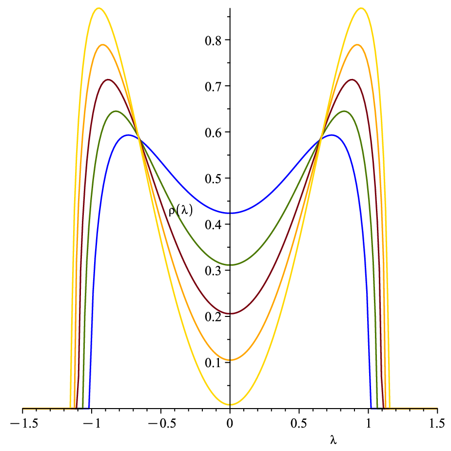
was studied. We will recall those results here as an example. In our paper [56], the phase transition location is off due to a missing scalar factor. In this paper we will give the new correct value that we have been able to derive analytically and have also verified with our own Monte Carlo simulations. Furthermore, the relationship between the coupling constant and the support is given by slightly different equations in both the single cut and double cut solutions. It was shown in [56] that the quartic $(1,0)$ and $(0,1)$ ensembles have the same behavior in the large $N$ limit. Using the Coulomb gas method as explained in Appendix A, we obtained the following explicit formula for the limiting eigenvalue density function of $H$: for $g>-4\sqrt{2}$,

$\displaystyle\rho(x)$

$\displaystyle=\frac{1}{\pi}(-4\gamma^{2}+\frac{1}{2\gamma^{2}}+4x^{2})\sqrt{4\gamma^{2}-x^{2}}_{[-2\gamma,2\gamma]},$

where the support $[-2\gamma,2\gamma]$ can be found as a function of $g$ as the root of

$\displaystyle 192\gamma^{8}+48\gamma^{4}+4g\gamma^{2}-1=0.$

When $g=-4\sqrt{2}$ the spectral phase transition occurs. For $g<-4\sqrt{2}$ the new limiting eigenvalue density function was found to be

$\displaystyle\begin{split}\rho(x)=\frac{2}{\pi}|x|\sqrt{(x^{2}-a^{2})(b^{2}-x^{2})}_{[-a,-b]\cup[b,a]},\end{split}$

where the support $[-a,-b]\cup[b,a]$ can be found in terms of $g$ via the equations

$$a^{2}=-\frac{1}{8}g+\frac{1}{\sqrt{2}},$$

and

$$b^{2}=-\frac{1}{8}g-\frac{1}{\sqrt{2}}.$$

These results are plotted in Figure 2.

As discussed in the previous section, the eigenvalue density function of the Dirac operator in the large $N$ limit is the convolution of the density functions of $H$. See Figure 3.

We note that the techniques presented in [56] in fact apply to any even potential Dirac ensembles of signature $(1,0)$ or $(0,1)$ and any convergent bi-tracial single matrix model. For example, let us consider the following type $(1,0)$ sextic model

$$Z=\int_{\mathcal{D}}e^{-\frac{g}{2}\tr D^{2}-\frac{1}{6}\tr D^{6}}dD.$$

Once again employing the Coulomb gas method results in the following explicit formula for the limiting eigenvalue density function:

$\displaystyle\rho(x)$

$\displaystyle=\frac{-40\,{{\gamma}}^{12}+20\,{{\gamma}}^{10}{x}^{2}+10\,{\gamma}^{8}{x}^{4}+50\,{{\gamma}}^{10}-50\,{{\gamma}}^{8}{x}^{2}+24\,{{\gamma}}^{6}-12\,{{\gamma}}^{4}{x}^{2}-{{\gamma}}^{2}{x}^{4}-1}{20\,{{\gamma}}^{8}\pi-2\,\pi\,{{\gamma}}^{2}}\sqrt{4\,{{\gamma}}^{2}-{x}^{2}}_{[-2\gamma,2\gamma]}$

where the support $[-2\gamma,2\gamma]$ can be found as a function of $g$ by (numerically) solving the equation

$\displaystyle 1=10\,\frac{{{\gamma}}^{2}\left(60\,{{\gamma}}^{16}-130\,{{\gamma}}^{14}-26\,{{\gamma}}^{10}-22\,{{\gamma}}^{8}+{{\gamma}}^{6}{g}-5\,{{\gamma}}^{4}-{g}/10\right)}{10\,{{\gamma}}^{6}-1}.$

Alternatively one can use the Lagrange inversion formula to find a perturbative expansion of $\gamma$ in terms of $g$. This model also exhibits at least one spectral phase transition and in general the plots are very similar to the quartic model. However, it is the belief of the authors that it might exhibit another phase transition, but further analysis is required. For details of this analysis, which is identical to the formal case, see the sextic example in [52].

In this subsection we shall very briefly give an overview of some of the results obtained in [6]. A simple, yet interesting, model of a discrete and finite noncommutative spin Riemannian manifold is a fuzzy spectral triple as we defined in Section 1. Given the important role that spectral geometry has played in global analysis, geometry, and topology of manifolds, as well as in noncommutative geometry, it is natural to ask to what extent its ideas can be extended to fuzzy spectral triples.

However, many of the results from spectral geometry are based on asymptotics of the spectrum $(\lambda_{n})_{n\in\mathbb{N}}$ of the Dirac operator $D$ (ordered such that $|\lambda_{n+1}|\geq|\lambda_{n}|$). Since the spectrum of the Dirac operator of a finite spectral triple is finite there is an obvious problem in directly generalizing such asymptotic results from spectral geometry to fuzzy spaces. For example, the first major result of spectral geometry is the celebrated Weyl’s asymptotic law, according to which the volume and dimension of a compact $d$-dimensional Riemanian manifold can be recovered from its Dirac spectrum:

$$\text{Vol}(M)=\lim_{n\rightarrow\infty}\frac{n\,(4\pi)^{d/2}\,\Gamma(1+d/2)}{k\,|\lambda_{n}|^{d}},$$

where $k$ is the rank of the spinor bundle of $M$ and $\Gamma(s)=\int_{0}^{\infty}e^{-t}\frac{t^{s}}{t}dt$ is the Gamma function.

In [6] the authors define, and numerically investigate, quantities computed from the spectrum that recover the usual asymptotic properties of dimension and volume for infinite spectra, but are also applicable to finite spectra. One such quantity is the spectral variance which is defined as

$$v_{s}(t)=2t^{2}\left(\frac{\sum_{i}\lambda_{i}^{4}e^{-\lambda_{i}^{2}t}}{\sum_{i}e^{-\lambda_{i}^{2}t}}-\left(\frac{\sum_{i}\lambda_{i}^{2}e^{-\lambda_{i}^{2}t}}{\sum_{i}e^{-\lambda_{i}^{2}t}}\right)^{2}\right).$$

If computed for the spectrum of a manifold one obtains $\lim_{t\to 0}v_{s}(t)=\dim(M)$, which follows from Weyl’s law. This quantity is also sensible for finite spectra, and gives the expected result of two for the fuzzy sphere and tori for appropriate values of $t$ [6]. The presence of the parameter $t$ should be thought of as an energy scale, with $t$ small corresponding to high energies and small wavelengths and $t$ large corresponding to low energies and large wavelengths. For fuzzy spaces $\lim_{t\to 0}v_{s}(t)=0$, as fuzzy spaces have a minimum wavelength, or Planck length, built in.

Another way to access asymptotic information in the spectrum $(\lambda_{n})$ is by the spectral zeta function

$$\zeta_{D}(s)=\sum_{n=1}^{\infty}\frac{1}{\lambda_{n}^{2s}},$$

which turns out to be useful even in the finite case. It is well-known that Weyl’s Law is equivalent to the fact that the volume of $M$ can be expressed in terms of the residue of the spectral zeta function $\zeta_{D}(s)$ at its top pole $s=d/2$:

$$\text{Vol}(M)=\frac{(4\pi)^{d/2}}{k}\text{Res}_{s=d/2}(\zeta_{D}(s)\Gamma(s)).$$

One can use the spectral zeta function to define a notion of distance between fuzzy spectral triples and even between fuzzy spectral triples and manifolds. One possibility for a notion of distance between metric spaces is the Gromov-Hausdorff distance [75], but in [31] the authors define a distance notion more useful in this situation, based on the spectra of Riemannian manifolds. Let $D_{1}$ and $D_{2}$ be two Dirac operators with $\zeta_{D_{1}}(s)$ and $\zeta_{D_{2}}(s)$ their spectral zeta functions. Then the distance between geometries is defined to be

$$\sigma(D_{1},D_{2})=\sup_{\gamma\leq s\leq\gamma+1}\left|\log\left(\frac{\zeta_{D_{1}}(s)}{\zeta_{D_{2}}(s)}\right)\right|$$

(4)

for some interval $[\gamma,\gamma+1]$ where all poles lie below $\gamma$. For Dirac operators on compact spin manifolds it was found in [31] that this is indeed a metric, in particular $\sigma(D_{1},D_{2})=0$ if and only if the spectra are the same.

In [6] this idea is adapted to define a distance between (random) fuzzy spectral triples. For example for each fuzzy sphere with matrix size $N$ we have a Dirac operator of size $N$. This spectrum is the same as the Dirac operator on the spin bundle of the 2-sphere tensored with $\mathbb{C}^{2}$ but with a cut-off. As $N$ goes to infinity the spectral zeta function of the fuzzy sphere converges to the spectral zeta function of the sphere uniformly on the interval $[\gamma,\gamma+1]$ for any $\gamma>1$. Thus, $\sigma(D_{N},D_{S^{2}})$ goes to zero as $N$ goes to infinity. Note that when considering truncated spectra, pointwise convergence of zeta functions is not a sufficient condition for $\sigma(D_{1},D_{2})=0$, uniform convergence is needed. For more on fuzzy spaces and truncated spectral triples see [45, 46].

One of the most remarkable results in [6] is that, when using the spectral distance to compare random spectra sampled from each of the quartic Dirac ensembles of types $(1,1)$, $(2,0)$, and $(1,3)$ to the fuzzy sphere for various values of the coupling constant, near the spectral phase transition the spectral distance $\sigma$ tends to zero. See Figure 5. The authors of [6] found further numerical evidence that, near spectral phase transitions, Dirac ensembles display manifold-like behavior, but we are still far from proving such a conjecture rigorously.

It has long been known that random matrix theory has connections to two dimensional quantum gravity. These range from the famous Kontsevich model [89, 58], to the newly discovered connections to Jackiw-Teitelboim (JT) gravity [78, 81, 90, 67]. Of particular interest however, is the connection to conformal field theory. Heuristically, physicists knew in the 80’s and 90’s from the asymptotics of convergent matrix integrals (found using orthogonal polynomials) that certain matrix ensembles have critical exponents corresponding to models in conformal field theories coupled to gravity [21, 36].

The idea is that matrix models count maps which can be thought of as discretized Riemann surfaces. If the coupling constants of the models are tweaked such that the number of polygons that form these maps goes to infinity, one would in essence be counting Riemann surfaces, which are also counted in conformal field theories in two dimensions. Later in [10], this idea was made precise with formal matrix models. These formal models often have the same asymptotics as their convergent matrix model counterparts (if such a counterpart exists). We will briefly describe the idea behind these critical points here.

Suppose a formal random matrix model’s partition function $Z$ has the following genus expansion

$$\log Z=\sum_{g\geq 0}N^{2-2g}\,F_{g},$$

where the $F_{g}$ are the generating functions of certain types of maps (specified by the model) with no boundaries [41], see Appendix B for details. Random matrix models often have critical points where the coupling constants of the model are such that the number of polygons in the maps goes to infinity. In such cases it is proven that the $F_{g}$ have asymptotic expansions around these points, which have critical exponents corresponding to a minimal model in conformal field theory [35, 10]. Additionally, these matrix model asymptotics satisfy a partial differential equation that is also satisfied by the corresponding minimal model. For example, the quartic Hermitian matrix model corresponds to the $(3,2)$ minimal model, also referred to as pure gravity, and its partition function satisfies Painlevé I.

How this relates to Dirac ensembles is not as obvious at a first glance. However, for several models examined in [52] we prove that single Hermitian matrix models are hidden in Dirac ensembles. In particular the cubic, quartic, and sextic Dirac ensembles of type $(1,0)$ contain the cubic, quartic, and sextic Hermitian matrix models, respectively, in their phase space. This is nontrivial because in a Dirac ensemble coupling constants are not attached to specific bi-tracial terms. Instead many single and bi-tracial terms share the same coupling constants, so one cannot easily turn off all bi-tracial terms by setting certain coupling constants to zero.

Consider for example the quartic Dirac ensemble from Section 1.3. As alluded to, one can fine-tune its coupling constants such that we recover a quartic Hermitian matrix model in the large $N$ limit. For a full proof see [52].

The single trace quartic model

$$\int_{\mathcal{H}_{N}}e^{-\frac{N}{2}\tr H^{2}-\frac{t_{4}}{4}N\tr H^{4}}dH$$

(5)

has a critical point at $t_{4}=-1/12$ which we will refer to as $t_{c}$ [41]. The singular parts of the $F_{g}$ are algebraic for all genus $g$, except for $g=1$, in which case it is logarithmic. In particular they are

$$\text{sing}(F_{g})=C_{g}\,(t_{4}-t_{c})^{5(1-g)/2}$$

and

$$\text{sing}(F_{1})=C_{1}\,\log(t_{4}-t_{c})$$

for $g\not=1$. These expansions are often referred to as a “double scaling limit”. We may define the generating series

$$u(y)=\sum_{g=0}^{\infty}C_{g}y^{5(1-g)/2}.$$

Then $u^{\prime\prime}(y)$ satisfies the Painlevé I equation, i.e.

$$y=(u^{\prime\prime}(y))^{2}-\frac{1}{3}u^{(4)}(y).$$

We know that the critical point of the quartic Hermitian model is $t_{4}=-1/12$ [41], and that the quartic Dirac ensemble

$$Z=\int_{\mathcal{D}}e^{-\frac{t_{2}}{4}\tr D^{2}-\frac{t_{4}}{8}\tr D^{4}}dD$$

(6)

contains it i.e. for a certain choice of coupling constants you recover the quartic Hermitian model. In particular, this happens when $t_{2}=4/3$ and $t_{4}=-1/12$ [52]. Figure 6 allows one to visualize several phenomena of the model in a phase diagram.

References

- [1] G. Anderson, A. Guionnet, and O. Zeitouni. An Introduction to Random Matrices. Cambridge: Cambridge University Press (Cambridge Studies in Advanced Mathematics). 2009.
- [2] P. Anderson and M. Kruczenski. Loop equation in Lattice gauge theories and bootstrap methods. EPJ Web Conf, 175 11011, 2018.
- [3] S. Azarfar and M. Khalkhali. Random Finite Noncommutative Geometries and Topological Recursion. arXiv:1906.09362.
- [4] J. W. Barrett. Matrix Geometries and Fuzzy Spaces as Finite Spectral Triples. J. Math. Phys., 56(8):082301, 25, 2015.
- [5] J. W. Barrett and L. Glaser. Monte Carlo Simulations of Random Non-commutative Geometries. J. Phys. A, 49(24):245001, 27, 2016.
- [6] J. W. Barrett, P. Druce, and L. Glaser. Spectral estimators for finite non-commutative geometries. J. Phys. A: Math. Theor., 52 275203, 2019.
- [7] J. W. Barrett and J. Gaunt. (2019). Finite spectral triples for the fuzzy torus. arXiv:1908.06796.
- [8] A. A. Belavin, A. Polyakov and A. B. Zamolodchikov. Infinite conformal symmetry in two-dimensional quantum field theory. Nuclear Physics B. 241 (2): 333-380, 1984.
- [9] D. Berenstein and G. Hulsey. Bootstrapping Simple QM Systems. arXiv:2108.08757.
- [10] M. Bergère and B. Eynard. Universal scaling limits of matrix models, and (p,q) Liouville gravity. arXiv:0909.0854.
- [11] J. Bhattacharya, D. Das, S. Kumar Das, A. Jha, and M. Kundu. Numerical bootstrap in quantum mechanics. Physics Letters B, Volume 823, 2021.
- [12] J. Bonifacio. Bootstrapping Closed Hyperbolic Surfaces. arXiv:2111.13215.
- [13] J. Bonifacio and K Hinterbichler. Bootstrap Bounds on Closed Einstein Manifolds. arXiv:2007.10337.
- [14] G. Borot. Formal multidimensional integrals, stuffed maps, and topological recursion. Annales de l’Institut Henri Poincaré D 1(2), Volume 1, Issue 2, 2014.
- [15] G. Borot and S. Shadrin. Blobbed topological recursion: properties and applications. Math. Proc. Cambridge Philos. Soc. 162, no. 1, 2017.
- [16] G. Borot, V. Bouchard, N. K. Chidambaram, T. Creutzig, and D. Noshchenko. Higher Airy structures, W algebras and topological recursion. arXiv:1812.08738.
- [17] J. Branahl, H. Grosse, A. Hock, and R. Wulkenhaar. Blobbed topological recursion of the quartic Kontsevich model I: Loop equations and conjectures. arXiv:2008.12201.
- [18] J. Branahl, H. Grosse, A. Hock, and R. Wulkenhaar. Perturbative and Geometric Analysis of the Quartic Kontsevich Model. SIGMA 17 085, 2021.
- [19] J. Branahl, H. Grosse, A. Hock, and R. Wulkenhaar. From scalar fields on quantum spaces to blobbed topological recursion. arXiv:2110.11789.
- [20] E. Brézin, C. Itzykson, G. Parisi and J.B. Zuber. Planar Diagrams. Commun. Math. Phys. 59, 35-51, 1978.
- [21] E. Brézin and V.A. Kazakov. Exactly solvable field theories of closed strings. Physics Letters B, 236 2, 144-150, 1990.
- [22] A. H. Chamseddine and A. Connes. The Spectral action principle. Commun. Math. Phys., 186:731–750, 1997.
- [23] A. H. Chamseddine, A. Connes, and M. Marcolli. Gravity and the standard model with neutrino mixing. Adv.Theor.Math.Phys., 11:991-1089,2007.
- [24] A. H. Chamseddine and W. van Suijlekom. A survey of spectral models of gravity coupled to matter. Advances in Noncommutative Geometry. Springer, 2019.
- [25] A. Connes. Geometry from the spectral point of view. Lett. Math. Phys., 34(3):203-238, 1995.
- [26] A. Connes. Noncommutative geometry and reality. J. Math. Phys. 36.11, 6194-6231, 1995.
- [27] A. Connes. Gravity coupled with matter and foundation of non-commutative geometry. Comm. Math. Phys. 182:155-176, 1996
- [28] A. Connes. On the spectral characterization of manifolds. J. Noncommut. Geom., 7(1):1-82, 2013.
- [29] A. Connes. Geometry and the Quantum. Foundations of mathematics and physics one century after Hilbert, pp. 159–196, Springer, Cham, 2018.
- [30] A. Connes and M. Marcolli. Noncommutative Geometry, Quantum Fields and Motives. American Mathematical Society, 2007.
- [31] G. Cornelissen and A. Kontogeorgis. Letters in Mathematical Physics. 107, 129 ISSN 0377-9017, 2017.
- [32] F. D’Andrea, F. Lizzi, and J. Varilly. Metric Properties of the Fuzzy Sphere. Lett.Math.Phys. 103, 183-205, 2013.
- [33] J. Daul, V. Kazakov and I. Kostov, Rational theories of 2-D gravity from the two matrix model. Nucl. Phys. B 409 311, 1991.
- [34] P. Deift. Orthogonal polynomials and random matrices: A Riemann-Hilbert approach. Courant lecture notes 3 New York: New York University. 1999.
- [35] P. Di Francesco, P.H. Ginsparg, and J. Zinn-Justin. 2-D Gravity and random matrices. Phys. Rept. 254, 1995.
- [36] M. R. Douglas and S. H. Shenker. Strings in less than one dimension. Nuclear Physics B, 335 3, 635-654, 1990.
- [37] B. Eynard. Formal matrix integrals and combinatorics of maps. math-ph/0611087. 2006.
- [38] B. Eynard and N. Orantin. Invariants of algebraic curves and topological expansion. arXiv:math-ph/0702045.
- [39] B. Eynard. A short overview of the “Topological recursion”. arXiv:1412.3286.
- [40] B. Eynard, T. Kimura, and S. Ribault. Random matrices. arXiv:1510.04430.
- [41] B. Eynard. Counting Surfaces, volume 70 of Progress in Mathematical Physics, Birkhäuser/Springer, CRM Aisenstadt chair lectures. 2016.
- [42] J. Gaunt, H. Nguyen, and A. Schenkel. BV quantization of dynamical fuzzy spectral triples. arXiv:2203.04817.
- [43] E. Gesteau. Renormalizing Yukawa interactions in the standard model with matrices and noncommutative geometry. J. Phys. A: Math. Theor., 54 035203, 2021.
- [44] L. Glaser. Scaling behaviour in random non-commutative geometries. J.Phys.A, 50 27, 275201, 2017.
- [45] L. Glaser and A. Stern. Understanding truncated non-commutative geometries through computer simulations. Journal of Mathematical Physics 61 (3), 033507, 2020.
- [46] L. Glaser and A. Stern. Reconstructing manifolds from truncations of spectral triples. J.Geom.Phys., 159 103921, 2021.
- [47] H. Grosse, C. Klimcik, and P. Presnajder. Towards finite quantum field theory in non-commutative geometry. arXiv arXiv:hep-th/9505175.
- [48] R. Gurau. Invitation to random tensors. SIGMA. Symmetry, Integrability and Geometry: Methods and Applications, 12, 094, 2014.
- [49] M. Hale. Path integral quantisation of finite noncommutative geometries. J. Geom. Phys. 44 115-128, 2002.
- [50] X. Han, S.A. Hartnoll and J. Kruthoff. Bootstrapping Matrix Quantum Mechanics. Phys. Rev. Lett, 125, 2020.
- [51] H. Hessam, M. Khalkhali and N. Pagliaroli. Bootstrapping Dirac Ensembles. J. Phys. A: Math. Theor. 55 335204, 2022.
- [52] H. Hessam, M. Khalkhali and N. Pagliaroli. Double scaling limits of Dirac ensembles and Liouville quantum gravity. Submitted to J. Phys. A: Math. Theor.
- [53] A. Hock and R. Wulkenhaar. Blobbed topological recursion of the quartic Kontsevich model II: Genus=0. arXiv:2103.13271.
- [54] R. Iseppi and W. van Suijlekom. Noncommutative geometry and the BV formalism: application to a matrix model. J.Geom.Phys. 120, 129-141, 2017.
- [55] V. Kazakov and Z. Zheng. Analytic and Numerical Bootstrap for One-Matrix Model and ”Unsolvable” Two-Matrix Model. arXiv:2108.04830.
- [56] M. Khalkhali and N. Pagliaroli. Phase transition in random noncommutative geometries. Journal of Physics A: Mathematical and Theoretical, Volume 54, Issue 3, id.035202, 2021.
- [57] M. Khalkhali and N. Pagliaroli. Spectral statistics of Dirac ensembles. J. Math. Phys. 63, 053504, 2022.
- [58] M. Kontsevich. Intersection theory on the moduli space of curves and the matrix Airy function. Commun.Math.Phys. 147, 1-23, 1992.
- [59] M. Kontsevich and Y. Soibelman. Airy structures and symplectic geometry of topological recursion. arXiv:1701.09137.
- [60] T. Krajewski. Classification of finite spectral triples. J. Geom. Phys., 28:1–30, 1998.
- [61] G. Landi, F. Lizzi, and R. J. Szabo. From Large N Matrices to the Noncommutative Torus. Com. Math. Phys. 217, 181-201, 1999.
- [62] F. Latrémolière. Convergence of Spectral Triples on Fuzzy Tori to Spectral Triples on Quantum Tori. Com. Math. Phys. 388, 1049–1128, 2021.
- [63] H.W. Lin. Bootstraps to strings: solving random matrix models with positivity. J. High Energ. Phys., 90, 2020.
- [64] E. Lira-Torres, and S. Majid. Geometric Dirac operator on the fuzzy sphere. Letters in Mathematical Physics, 112(1), 1-22, 2022.
- [65] J. Madore. The Fuzzy sphere. Class.Quant.Grav. 9 69-88, 1991.
- [66] M. Marcolli. Noncommutative Cosmology. World Scientific, 2019.
- [67] H. Maxfield and G. J. Turiaci. The path integral of 3D gravity near extremality; or, JT gravity with defects as a matrix integral. Journal of High Energy Physics, 118 2021.
- [68] A. A. Migdal. Loop Equations and 1/N Expansion. Phys. Rept, 102 199–290, 1984.
- [69] A. Perez. The spin-foam approach to quantum gravity. Living Reviews in Relativity 16.1, 1-128, 2013.
- [70] C. Perez-Sanchez. Computing the spectral action for fuzzy geometries: from random noncommutatative geometry to bi-tracial multimatrix models. arXiv:1912.13288.
- [71] C. Perez-Sanchez. On multimatrix models motivated by random Noncommutative Geometry I: the Functional Renormalization Group as a flow in the free algebra. Annales Henri Poincaré, 22 3095–3148, 2021.
- [72] C. Perez-Sanchez. On multimatrix models motivated by random Noncommutative Geometry II: A Yang-Mills-Higgs matrix model. Annales Henri Poincaré, 23, 1979–2023, 2022.
- [73] R. Rattazzi, V.S. Rychkov, E. Tonni and A. Vichi. Bounding scalar operator dimensions in 4D CFT. Journal of High Energy Physics 031 0807.0004, 2008.
- [74] M. Reed and B. Simon. Fourier Analysis, Self-Adjointness. Methods of modern mathematical physics, 2. Academic Press, 1975.
- [75] M. A. Rieffel. Gromov-Hausdorff Distance for Quantum Metric Spaces/matrix Algebras Converge to the Sphere for Quantum Gromov-Hausdorff Distance. American Mathematical Soc., 168, 796, 2004.
- [76] C. Rovelli, and L. Smolin. Spin networks and quantum gravity. Physical Review D 52 10 5743, 1995.
- [77] C. Rovelli. Loop quantum gravity. Living reviews in relativity, 11.1, 1-69, 2008.
- [78] P. Saad, S. H. Shenker, and D. Stanford. JT gravity as a matrix integral. arXiv:1903.11115.
- [79] P. Schreivogl and H.Steinacker, H.. Generalized fuzzy torus and its modular properties. SIGMA. Symmetry, Integrability and Geometry: Methods and Applications, 9, 060, 2013.
- [80] J. Schürmann and R. Wulkenhaar. An algebraic approach to a quartic analogue of the Kontsevich model. arXiv:1912.03979.
- [81] D. Stanford and E. Witten. JT gravity and the ensembles of random matrix theory. Adv. Theor. Math. Phys. 24, 1475, 2020.
- [82] R. L. Stratonovich. On distribution in representation space. Sov. Phys. JETP 4, 891–898, 1957.
- [83] T. D. H. van Nuland and W. D. van Suijlekom. One-loop corrections to the spectral action. Journal of High Energy Physics. 78 2022.
- [84] W. D. van Suijlekom. Noncommutative Geometry and Particle Physics. Springer, 2014.
- [85] J. C. Várilly, J. Gracia-Bondía. The moyal representation for spin. Ann. Phys. 190, 1, 107-148, 1989.
- [86] E. Wigner. Characteristic vectors of bordered matrices with infinite dimensions. Ann. of Math. 3 62, 548-564, 1955.
- [87] E. Wigner. Characteristic vectors of bordered matrices of infinite dimensions II. Ann. of Math. 2 65, 203-207, 1957.
- [88] E. Wigner. On the distribution of the roots of certain symmetric matrices. Ann. of Math. 2 67, 325-326, 1958.
- [89] E, Witten. Two-dimensional gravity and intersection theory on moduli space. Surveys in differential geometry, vol. 1, Bethlehem, PA: Lehigh Univ., 243–310, 1990.
- [90] E. Witten. Matrix Models and Deformations of JT Gravity. Proceedings of the Royal Society A, 2020.