On the shape of the first fractional eigenfunctionThanks: MSC2020: Primary: 47A75, 35B99, 35P05; Secondary: 47G20, 35R11. Thanks: Acknowledgements: The first author has been partially supported by the Alexander von Humboldt Foundation.

Nicola Abatangelo Address: (N. Abatangelo) Dipartimento di Matematica, Alma Mater Studiorum Università di Bologna, P.zza di Porta S. Donato 5, 40126 Bologna, Italy. Email address: nicola.abatangelo@unibo.it and Sven Jarohs Address: (S. Jarohs) Institut für Mathematik, Goethe-Universität Frankfurt am Main, Robert-Meyer-Str. 10, 60325 Frankfurt am Main, Germany. Email address: jarohs@math.uni-frankfurt.de

Date: August 11, 2026

Abstract.

We show that the first eigenfunction of the fractional Laplacian ${\left(-\Delta\right)}^{s}$ , $s\in(1/2,1)$ , is superharmonic in the unitary ball up to dimension $11$ . To this aim, we also rely on a computer-assisted step to estimate a rather complicated constant depending on the dimension and the power $s$ .

1. Introduction

The fractional Laplace operator is an integro-differential nonlocal operator of non-integer order. It is defined as

\displaystyle{\left(-\Delta\right)}^{s}u(x)

\displaystyle:=\frac{4^{s}\Gamma(n/2+s)}{\pi^{n/2}\big|\Gamma(-s)\big|}\;\mathrm{p.v.}\!\!\int_{\mathbb{R}^{n}}\frac{u(x)-u(y)}{{|x-y|}^{n+2s}}\;dy

\displaystyle s\in(0,1),\ x\in\mathbb{R}^{n},

where “ $\mathrm{p.v.}\!\!$ ” means that the integral is taken in the principal value sense. We refer to [10, 7, 1, 12] for all its basic features.

Here, we recall that it is naturally related to the fractional Sobolev space

\displaystyle H^{s}(\mathbb{R}^{n})=\left\{u\in L^{2}(\mathbb{R}^{n}):[u]^{2}_{s}:=\int_{\mathbb{R}^{n}}\int_{\mathbb{R}^{n}}\frac{{|u(x)-u(y)|}^{2}}{{|x-y|}^{n+2s}}\;dy\;dx<\infty\right\}

and, when the attention is restricted to a bounded domain $\Omega\subset\mathbb{R}^{n}$ , to the space

\displaystyle{\mathcal{H}}^{s}_{0}(\Omega)=\big\{u\in H^{s}(\mathbb{R}^{n}):u=0\text{ in }\mathbb{R}^{n}\setminus\Omega\big\},

which is encoding a natural notion of homogeneous boundary conditions in $\mathbb{R}^{n}\setminus\Omega$ : for this reason it is sometimes also known as the restricted fractional Laplacian. From a functional analytic perspective, ${\left(-\Delta\right)}^{s}$ is a positive self-adjoint operator on $\{u\in L^{2}(\mathbb{R}^{n}):u=0\text{ in }\mathbb{R}^{n}\}$ with compact inverse. It has therefore a discrete spectrum and the eigenvalues have finite multiplicity. In particular, the first eigenvalue, which we denote by $\lambda=\lambda(\Omega)$ , is simple. It is known that the first eigenfunction $\phi\in{\mathcal{H}}^{s}_{0}(\Omega)$ is smooth inside $\Omega$ and that it can be chosen to be strictly positive.

In this paper we partially answer a conjecture raised by Bañuelos, Kulczycki, and Méndez-Hernández [5]*Conjecture 1.1:

(1.1)

n=1

and

\Omega=(-1,1)

, then

\phi

is concave in its support.

This has been previously established by Bañuelos and Kulczycki [6]*Theorem 4.7, for $s=\frac{1}{2}$ , and by Kaßmann and Silvestre [13] and Bañuelos and DeBlassie [4]*Theorem 1.1, whenever $s^{-1}\in\mathbb{N}$ ; moreover, in general dimension and for a general bounded Lipschitz domain, [4]*Theorem 1.1 also shows that $\phi$ is superharmonic, again under the assumption $s^{-1}\in\mathbb{N}$ . Another related result is contained in [5]*Theorem 1.1, which states that $\phi$ is mid-concave (see [5]*Definition 1.1) on rectangles $\Omega=(-a_{1},a_{1})\times\cdots\times(-a_{n},a_{n})\subset\mathbb{R}^{n}$ .

Here, we give a computer-aided proof of (1.1) for any $s\in(\frac{1}{2},1)$ .

Theorem 1.1.

Let $s\in(\frac{1}{2},1)$ and $n=1$ . Let $\phi\in{\mathcal{H}}^{s}_{0}\big((-1,1)\big)$ denote the first eigenfunction of ${\left(-\Delta\right)}^{s}$ on the interval $(-1,1)$ . Then

\displaystyle\phi^{\prime\prime}<0\qquad\text{in }(-1,1).

More generally, our approach is able to reach the following.

Theorem 1.2.

Let $s\in(\frac{1}{2},1)$ , $2\leq n\leq 11$ , and $B_{1}\subset\mathbb{R}^{n}$ denote the unitary ball. Let $\phi\in{\mathcal{H}}^{s}_{0}(B_{1})$ denote the first eigenfunction of ${\left(-\Delta\right)}^{s}$ on $B_{1}$ . Then

(1.2)

\displaystyle-\Delta\phi>0\qquad\text{in }B_{1}.

We believe the threshold $n\leq 11$ to be merely technical and due to a few sub-optimal estimates involved in our analysis.

Our strategy begins with a purely analytic approach to reduce $\Delta\phi$ in an integral form. At the core of this strategy we exploit the semigroup property of ${\left(-\Delta\right)}^{s}$ in that we split

	$\displaystyle-\Delta\phi$	$\displaystyle={(-\Delta)}^{1-s}{\left(-\Delta\right)}^{s}\phi={(-\Delta)}^{1-s}\big(\lambda\phi+\mathbf{1}_{\mathbb{R}^{n}\setminus B_{1}}{\left(-\Delta\right)}^{s}\phi\big)$
(1.3)			$\displaystyle=\lambda{(-\Delta)}^{1-2s}\big(\lambda\phi+\mathbf{1}_{\mathbb{R}^{n}\setminus B_{1}}{\left(-\Delta\right)}^{s}\phi\big)+{(-\Delta)}^{1-s}\big(\mathbf{1}_{\mathbb{R}^{n}\setminus B_{1}}{\left(-\Delta\right)}^{s}\phi\big)$	$\displaystyle\qquad\text{in }B_{1}.$

Next, we write suitable integral representations for the different terms that appear: these use in a crucial way our standing assumption $s>\frac{1}{2}$ , so that $(-\Delta)^{1-2s}$ stands for the convolution with the fundamental solution in $\mathbb{R}^{n}$ . A central role in these formulas is played by the nonlocal Poisson kernel of $B_{1}$

(1.4)

\displaystyle P_{s}(x,y):=\frac{\gamma(n,s)}{{|x-y|}^{n}}\frac{\big(1-|x|^{2}\big)^{s}}{\big(|y|^{2}-1\big)^{s}},\quad\gamma(n,s):=\frac{\Gamma(\frac{n}{2})}{\pi^{n/2}\Gamma(s)\,\Gamma(1-s)},\qquad x\in B_{1},\ y\in\mathbb{R}^{n}\setminus B_{1}.

The splitting of $-\Delta\phi$ is performed in Section 2. A refinement of (1.3) leads to write (1.2) as an integral inequality not involving directly $\phi$ or $\lambda$ (see (2.8) below). At this point we split our analysis in three different cases:

•

For $n=1$ and $s=\frac{3}{4}$ the argument can be concluded by hand, without too much of a hustle: this is done in Section 3.
•

For $n=1$ and $s\in(\frac{1}{2},1)\setminus\{\frac{3}{4}\}$ the integral quantities can be simplified a lot via estimates from below; still, the resulting inequality contains a quite complicated expression in $s$ and we therefore plot and verify it using a computer: this is done in Section 4;
•

For $n\geq 2$ a similar approach to the previous point is taken, with the important difference that in this case hypergeometric functions make their appearance in our study: these make the analysis even more complicated and we consequently need to rely even more on numerical evaluations: this is done in Section 5.

Many details will be deferred to Appendices, in the attempt of not breaking the flow of the exposition with technicalities. Nevertheless, we would like to mention that in Appendix B we derive an upper bound for the first eigenvalue $\lambda$ on $B_{1}$ for general dimension $n$ and power $s$ , while in Appendix C we derive from a representation formula for certain $s$ -harmonic functions some symmetry and monotonicity properties which are useful in our analysis and might be of independent interest.

1.1. Notations

We denote by $B_{r}$ the $n$ -dimensional ball of radius $r>0$ centered at $0$ . We set

(1.5)

\displaystyle F_{\tau}(z)

\displaystyle:=\left\{\begin{aligned} &\kappa(n,\tau)|z|^{2\tau-n},\quad\kappa(n,\tau):=\frac{\Gamma(\frac{n}{2}-\tau)}{4^{\tau}\pi^{n/2}\big|\Gamma(\tau)\big|},&&\tau\in\mathbb{R},\ \tau-\frac{n}{2}\not\in\mathbb{N}_{0},\\ &(-1)^{1+\tau-n/2}\frac{2^{1-2\tau}\pi^{-n/2}}{\Gamma(1+\tau-\frac{n}{2})\,\Gamma(\tau)}\,|z|^{2\tau-n}\,\ln|z|,&&\tau\in\mathbb{R},\ \tau-\frac{n}{2}\in\mathbb{N}_{0},\end{aligned}\right.

\displaystyle z\in\mathbb{R}^{n}\setminus\{0\}.

Note that $F_{\tau}$ is the fundamental solution of $(-\Delta)^{\tau}$ in $\mathbb{R}^{n}$ if $\tau>0$ and for $\tau\in(-1,0)$ it is the kernel of the fractional Laplacian of order $2\tau$ . For a measurable set $A\subset\mathbb{R}^{n}$ , $\mathbf{1}_{A}$ denotes the characteristic function of $A$ and $A^{c}=\mathbb{R}^{n}\setminus A$ the complementary set of $A$ .

2. Set-up of the proof of Theorems 1.1 and 1.2

2.1. Representation of the Laplacian of the eigenfunction

In this paragraph we perform the splitting of $-\Delta\phi$ announced in (1.3).

Lemma 2.1.

For $s\in(0,1)$ it holds ${\left(-\Delta\right)}^{s}\phi\in L^{1}(\mathbb{R}^{n})$ and we have

(2.1)

\displaystyle{\left(-\Delta\right)}^{s}\phi=\lambda\phi-\mathbf{1}_{B_{1}^{c}}(F_{-s}\ast\phi)\qquad\text{in }\mathbb{R}^{n}\setminus\partial B_{1}.

Proof.

Consider $\psi\in C^{\infty}_{c}(\mathbb{R}^{n})$ . Then

\displaystyle\int_{\mathbb{R}^{n}}\phi\,{\left(-\Delta\right)}^{s}\psi

\displaystyle=\int_{B_{1}}\phi\,{\left(-\Delta\right)}^{s}\mathbb{G}_{s}[{\left(-\Delta\right)}^{s}\psi]=\lambda\int_{B_{1}}\phi\,\mathbb{G}_{s}[{\left(-\Delta\right)}^{s}\psi]

Above, we have denoted by $\mathbb{G}_{s}:L^{2}(B_{1})\to{\mathcal{H}}^{s}_{0}(B_{1})$ the solution map to the Dirichlet problem

\displaystyle\left\{\begin{aligned} {\left(-\Delta\right)}^{s}u&=f&&\text{in }B_{1},\ f\in L^{2}(B_{1}),\\ u&\in{\mathcal{H}}^{s}_{0}(B_{1}),\end{aligned}\right.

which admits a representation in terms of the Green function

	$\displaystyle\mathbb{G}_{s}[f](x)$	$\displaystyle=\int_{B_{1}}G_{s}(x,y)\,f(y)\;dy$		$\displaystyle\text{for }x\in B_{1},$
	$\displaystyle G_{s}(x,y)$	$\displaystyle=F_{s}(x-y)-\int_{B_{1}^{c}}P_{s}(x,z)\,F_{s}(z-y)\;dz$		$\displaystyle\text{for }x,y\in B_{1},$
(2.2)		$\displaystyle P_{s}(x,y)$	$\displaystyle=\int_{B_{1}}F_{-s}(z-y)\,G_{s}(x,z)\;dz$		$\displaystyle\text{for }x\in B_{1},\ y\in B_{1}^{c},$

see [8]*Definition 1.9 and [2]*equation (25) and Theorem 1.2. We have then

	$\displaystyle\frac{1}{\lambda}\int_{\mathbb{R}^{n}}\phi\,{\left(-\Delta\right)}^{s}\psi$	$\displaystyle=\int_{B_{1}}\phi(x)\int_{B_{1}}F_{s}(x-y)\,{\left(-\Delta\right)}^{s}\psi(y)\;dy\;dx$
		$\displaystyle\quad-\int_{B_{1}}\phi(x)\int_{B_{1}^{c}}P_{s}(x,z)\int_{B_{1}}F_{s}(z-y)\,{\left(-\Delta\right)}^{s}\psi(y)\;dy\;dz\;dx$
		$\displaystyle=\int_{B_{1}}\phi\psi-\int_{B_{1}}\phi(x)\int_{B_{1}^{c}}F_{s}(x-y)\,{\left(-\Delta\right)}^{s}\psi(y)\;dy\;dx$
		$\displaystyle\quad-\int_{B_{1}}\phi(x)\int_{B_{1}^{c}}P_{s}(x,z)\,\psi(z)\;dz\;dx$
		$\displaystyle\quad+\int_{B_{1}}\phi(x)\int_{B_{1}^{c}}P_{s}(x,z)\int_{B_{1}^{c}}F_{s}(z-y)\,{\left(-\Delta\right)}^{s}\psi(y)\;dy\;dz\;dx$
		$\displaystyle=\int_{B_{1}}\phi\psi-\int_{B_{1}}\phi(x)\int_{B_{1}^{c}}P_{s}(x,z)\,\psi(z)\;dz\;dx$
		$\displaystyle\quad+\int_{B_{1}}\phi(x)\int_{B_{1}^{c}}\bigg(\int_{B_{1}^{c}}P_{s}(x,z)\,F_{s}(z-y)\;dz-F_{s}(x-y)\bigg){\left(-\Delta\right)}^{s}\psi(y)\;dy\;dx.$

As it holds (see [14]*equation (1.6.12’))

\displaystyle\int_{B_{1}^{c}}P_{s}(x,z)F_{s}(z-y)\;dz=F_{s}(x-y)\qquad\text{for }x\in B_{1},\ y\in B_{1}^{c},

then

	$\displaystyle\int_{\mathbb{R}^{n}}\phi\,{\left(-\Delta\right)}^{s}\psi$	$\displaystyle=\lambda\int_{B_{1}}\phi\,\psi-\lambda\int_{B_{1}}\phi(x)\int_{B_{1}^{c}}P_{s}(x,z)\,\psi(z)\;dz\;dx$
		$\displaystyle=\lambda\int_{B_{1}}\phi\,\psi-\int_{B_{1}^{c}}\psi(z)\int_{B_{1}}P_{s}(x,z)\,\lambda\phi(x)\;dx\;dz$
(2.3)			$\displaystyle=\lambda\int_{B_{1}}\phi\,\psi-\int_{B_{1}^{c}}\psi\,(F_{-s}\ast\mathbb{G}_{s}[\lambda\phi])=\lambda\int_{B_{1}}\phi\,\psi-\int_{B_{1}^{c}}\psi\,(F_{-s}\ast\phi)$

where we have used (2.2). The stated equality (2.1) holds also pointwisely in view of [17]*Proposition 2.4. ∎

Proposition 2.2.

For $s\in(\frac{1}{2},1)$ it holds

(2.4)		$\displaystyle-\Delta\phi$	$\displaystyle=\lambda^{2}F_{2s-1}\ast\phi+\big(F_{s-1}-\lambda F_{2s-1}\big)\ast\big[\mathbf{1}_{B_{1}^{c}}(F_{-s}\ast\phi)\big]$
(2.5)			$\displaystyle=\lambda^{2}F_{2s-1}\ast\phi+\lambda\big(F_{s-1}-\lambda F_{2s-1}\big)\ast\mathbf{P}_{s}[\phi]$	$\displaystyle\text{in }B_{1},$

where

\displaystyle\mathbf{P}_{s}[\phi](y)=\mathbf{1}_{B_{1}^{c}}(y)\int_{B_{1}}P_{s}(x,y)\,\phi(x)\;dx\qquad\text{for }y\in\mathbb{R}^{n}.

Proof.

Starting from the last lemma, we compute (all equalities hold only in $B_{1}$ )

\displaystyle-\Delta\phi={(-\Delta)}^{1-s}{\left(-\Delta\right)}^{s}\phi={(-\Delta)}^{1-s}\big[\lambda\phi-\mathbf{1}_{B_{1}^{c}}(F_{-s}\ast\phi)\big]=\lambda{(-\Delta)}^{1-s}\phi+F_{s-1}\ast[\mathbf{1}_{B_{1}^{c}}(F_{-s}\ast\phi)].

Note that

\displaystyle{(-\Delta)}^{1-s}\phi=F_{2s-1}\ast{\left(-\Delta\right)}^{s}\phi=F_{2s-1}\ast\big[\lambda\phi-\mathbf{1}_{B_{1}^{c}}(F_{-s}\ast\phi)\big]

thus (2.4) follows. In expanded form, (2.4) reads, for $x\in B_{1}$ ,

	$\displaystyle-\Delta\phi(x)$	$\displaystyle=\lambda^{2}\int_{B_{1}}F_{2s-1}(x-y)\,\phi(y)\;dy$
		$\displaystyle\qquad+\int_{B_{1}^{c}}\big(F_{s-1}(x-z)-\lambda F_{2s-1}(x-z)\big)\int_{B_{1}}F_{-s}(z-y)\,\phi(y)\;dy\;dz$
		$\displaystyle=\int_{B_{1}}\phi(y)\bigg[\lambda^{2}F_{2s-1}(x-y)+\int_{B_{1}^{c}}\big(F_{s-1}(x-z)-\lambda F_{2s-1}(x-z)\big)F_{-s}(z-y)\;dz\bigg]\;dy.$

Also, identity

\displaystyle(F_{-s}\ast\phi)(z)=\lambda\int_{B_{1}}P_{s}(y,z)\,\phi(y)\;dy\qquad\text{for }z\in B_{1}^{c},

holds (we have already used this one in (2.3) exploiting (2.2)). In expanded form, (2.5) reads

	$\displaystyle-\Delta\phi(x)$	$\displaystyle=\lambda^{2}\int_{B_{1}}F_{2s-1}(x-y)\,\phi(y)\;dy$
		$\displaystyle\qquad+\lambda\int_{B_{1}^{c}}\big(F_{s-1}(x-z)-\lambda F_{2s-1}(x-z)\big)\int_{B_{1}}P_{s}(y,z)\,\phi(y)\;dy\;dz$
		$\displaystyle=\lambda\int_{B_{1}}\phi(y)\bigg[\lambda F_{2s-1}(x-y)+\int_{B_{1}^{c}}P_{s}(y,z)\big(F_{s-1}(x-z)-\lambda F_{2s-1}(x-z)\big)\;dz\bigg]\;dy.$

∎

We know that, by uniqueness, $\phi$ and $-\Delta\phi$ are radial, so that for any $x\in B_{1}$ fixed

\displaystyle-\Delta\phi(x)=-\frac{1}{\big|\partial B_{|x|}\big|}\int_{\partial B_{|x|}}\Delta\phi(\theta)\;d\theta.

Keeping this in mind, we define

(2.6)

\displaystyle J_{\tau}(x;y):=\left\{\begin{aligned} &\frac{1}{\big|\partial B_{|x|}\big|}\int_{\partial B_{|x|}}F_{\tau}(\theta-y)\;d\theta&&\text{for }n\geq 2,\,x,y\in\mathbb{R}^{n},\,x\neq y\\ &\frac{F_{\tau}(x-y)+F_{\tau}(x+y)}{2}&&\text{for }n=1,\,x,y\in\mathbb{R},\,x\neq y.\end{aligned}\right.

Using (2.5), we then write

\displaystyle-\Delta\phi(x)

\displaystyle=\lambda\int_{B_{1}}\phi(y)\bigg[\lambda J_{2s-1}(x;y)+\int_{B_{1}^{c}}P_{s}(y,z)\big(J_{s-1}(x;z)-\lambda J_{2s-1}(x;z)\big)\;dz\bigg]\;dy,\quad x\in B_{1}.

Since

\lambda J_{2s-1}(x;y)+\int_{B_{1}^{c}}P_{s}(y,z)\big(J_{s-1}(x;z)-\lambda J_{2s-1}(x;z)\big)\;dz=\\ =\lambda\bigg(J_{2s-1}(x;y)-\int_{B_{1}^{c}}P_{s}(y,z)\,J_{2s-1}(x;z)\;dz\bigg)+\int_{B_{1}^{c}}P_{s}(y,z)\,J_{s-1}(x;z)\;dz,

the positivity of $-\Delta\phi$ follows once we show

\displaystyle\lambda\bigg(J_{2s-1}(x;y)-\int_{B_{1}^{c}}P_{s}(y,z)\,J_{2s-1}(x;z)\;dz\bigg)+\int_{B_{1}^{c}}P_{s}(y,z)\,J_{s-1}(x;z)\;dz

\displaystyle\geq 0,\qquad x,y\in B_{1}.

As the second addend is clearly positive in the above inequality, we may replace $\lambda$ with a larger constant (see Appendix B, equation (B.1))

(2.7)

\displaystyle\lambda\leq\Lambda(n,s):=\frac{4^{s}\Gamma(1+s)^{2}\,\Gamma(1+2s+\frac{n}{2})}{(s+\frac{n}{2})\,\Gamma(\frac{n}{2})\,\Gamma(1+2s)}

and it is then enough to show

(2.8)

J_{2s-1}(x;y)-\int_{B_{1}^{c}}P_{s}(y,z)\,J_{2s-1}(x;z)\;dz+\frac{1}{\Lambda(n,s)}\int_{B_{1}^{c}}P_{s}(y,z)\,J_{s-1}(x;z)\;dz\geq 0,\\ s\in\Big(\frac{1}{2},1\Big),\ x,y\in B_{1}.

Note that $s-1-\frac{n}{2}<0$ for all $n\in\mathbb{N}$ and $s\in(\frac{1}{2},1)$ , but $2s-1-\frac{n}{2}\in\mathbb{N}_{0}$ if and only if $s=\frac{3}{4}$ and $n=1$ . Hence, this case differs strongly from the other cases as an effect of definitions (1.5) and (2.6). We begin with some general estimates to simplify (2.8).

2.2. Reformulation of (2.8)

The first step is to note that the left-hand side of (2.8) actually depends only on $|x|$ and $|y|$ .

Lemma 2.3.

For any $n\in\mathbb{N}$ , $\tau\in\mathbb{R}$ , and $s\in(0,1)$ we have

	$\displaystyle J_{\tau}(x;y)$	$\displaystyle=J_{\tau}(\|x\|e_{1},\|y\|e_{1})$		$\displaystyle x,y\in\mathbb{R}^{n},\,x\neq y,$
	$\displaystyle\int_{B_{1}^{c}}P_{s}(y,z)J_{\tau}(x;z)\ dz$	$\displaystyle=\int_{B_{1}^{c}}P_{s}(\|y\|e_{1},z)\,J_{\tau}(\|x\|e_{1};z)\;dz$		$\displaystyle x,y\in B_{1},\,x\neq y.$

Proof.

First note that $F_{\tau}(x)=F_{\tau}(|x|e_{1})$ for any $x\in\mathbb{R}^{n}\setminus\{0\}$ by definition (1.5). To see the statement for $J_{\tau}$ , note that this is obviously true for $n=1$ from definition (2.6) and for $n>1$ we have by a rotation for $x\in B_{1}$ , $y\in\mathbb{R}^{n}\setminus\{x\}$

		$\displaystyle J_{\tau}(x;y)=\frac{1}{\|\partial B_{\|x\|}\|}\int_{\partial B_{\|x\|}}F_{\tau}\big(\|\theta-y\|e_{1}\big)\;d\theta=\frac{1}{\|\partial B_{\|x\|}\|}\int_{\partial B_{\|x\|}}F_{\tau}\Big(\sqrt{1-2\theta\cdot y+\|y\|^{2}}\,e_{1}\Big)\;d\theta$
		$\displaystyle=\frac{1}{\|\partial B_{\|x\|}\|}\int_{\partial B_{\|x\|}}F_{\tau}\Big(\sqrt{1-2\|y\|\nu_{1}+\|y\|^{2}}e_{1})\;d\nu=\frac{1}{\|\partial B_{\|x\|}\|}\int_{\partial B_{\|x\|}}F_{\tau}\big(\nu-\|y\|e_{1}\big)\;d\nu=J_{\tau}(\|x\|e_{1};\|y\|e_{1}).$

Similarly, we have with a rotation

	$\displaystyle\int_{B_{1}^{c}}P_{s}(y,z)\,J_{\tau}(x;z)\;dz$	$\displaystyle=\frac{\Gamma(\frac{n}{2})}{\pi^{\frac{n}{2}}\Gamma(s)\Gamma(1-s)}\int_{B_{1}^{c}}\frac{(1-\|y\|^{2})^{s}}{(\|z\|^{2}-1)^{s}\|y-z\|^{n}}\,J_{\tau}(\|x\|e_{1};\|z\|e_{1})\;dz$
		$\displaystyle=\frac{\Gamma(\frac{n}{2})}{\pi^{\frac{n}{2}}\Gamma(s)\Gamma(1-s)}\int_{B_{1}^{c}}\frac{(1-\|y\|^{2})^{s}}{(\|z\|^{2}-1)^{s}\big(\|y\|^{2}-2y\cdot z+\|z\|^{2}\big)^{\frac{n}{2}}}\,J_{\tau}(\|x\|e_{1};\|z\|e_{1})\;dz$
		$\displaystyle=\frac{\Gamma(\frac{n}{2})}{\pi^{\frac{n}{2}}\Gamma(s)\Gamma(1-s)}\int_{B_{1}^{c}}\frac{(1-\|y\|^{2})^{s}}{(\|v\|^{2}-1)^{s}\big(\|y\|^{2}-2\|y\|v_{1}+\|v\|^{2}\big)^{\frac{n}{2}}}\,J_{\tau}(\|x\|e_{1};\|v\|e_{1})\;dv$
		$\displaystyle=\frac{\Gamma(\frac{n}{2})}{\pi^{\frac{n}{2}}\Gamma(s)\Gamma(1-s)}\int_{B_{1}^{c}}\frac{(1-\|y\|^{2})^{s}}{(\|v\|^{2}-1)^{s}\big\|\|y\|e_{1}-v\big\|^{n}}\,J_{\tau}(\|x\|e_{1};\|v\|e_{1})\;dv$
		$\displaystyle=\int_{B_{1}^{c}}P_{s}(\|y\|e_{1},v)\,J_{\tau}(\|x\|e_{1};v)\;dv.$

∎

In view of the last lemma (2.8) reduces to

J_{2s-1}(|x|e_{1};|y|e_{1})-\int_{B_{1}^{c}}P_{s}(|y|e_{1},z)\,J_{2s-1}(|x|e_{1};z)\;dz+\frac{1}{\Lambda(n,s)}\int_{B_{1}^{c}}P_{s}(|y|e_{1},z)\,J_{s-1}(|x|e_{1};z)\;dz\geq 0,\\ s\in\Big(\frac{1}{2},1\Big),\ x,y\in B_{1}.

Lemma 2.4.

Let $n\geq 2$ . For $\varepsilon,r>0$ and $\alpha\in\mathbb{R}$ it holds

\displaystyle\int_{\partial B_{r}}\frac{dx}{\big|x-\varepsilon e_{1}\big|^{2\alpha}}=\frac{2\pi^{\frac{n-1}{2}}}{\Gamma(\frac{n-1}{2})}\,r^{n-1}\int_{-1}^{1}\frac{(1-t^{2})^{\frac{n-3}{2}}}{\big(r^{2}+\varepsilon^{2}-2\varepsilon rt\big)^{\alpha}}\;dt

In case $r=\varepsilon$ , we additionally require $2\alpha<n-1$ . In particular, we have for $\tau-\frac{n}{2}\notin\mathbb{N}_{0}$

J_{\tau}(x;y)=\frac{2\pi^{\frac{n-1}{2}}}{\Gamma(\frac{n-1}{2})}\,\kappa(n,\tau)|x|^{n-1}\int_{-1}^{1}\frac{(1-t^{2})^{\frac{n-3}{2}}}{\big(|x|^{2}+|y|^{2}-2|x||y|t\big)^{\frac{n}{2}-\tau}}\;dt\qquad x,y\in\mathbb{R}^{n},

where we require additionally $|x|\neq|y|$ if $\tau>\frac{1}{2}$ .

Proof.

Via an explicit calculation

\int_{\partial B_{r}}\frac{dx}{\big|x-\varepsilon e_{1}\big|^{2\alpha}}=r^{n-1}\int_{\partial B_{1}}\frac{dy}{\big|ry-\varepsilon e_{1}\big|^{2\alpha}}=r^{n-1}\int_{\partial B_{1}}\frac{dy}{\big(r^{2}-2r\varepsilon y_{1}+\varepsilon^{2}\big)^{\alpha}}=\\ =\frac{2\pi^{\frac{n-1}{2}}}{\Gamma(\frac{n-1}{2})}\,r^{n-1}\int_{-1}^{1}\frac{(1-t^{2})^{\frac{n-3}{2}}}{\big(r^{2}+\varepsilon^{2}-2\varepsilon rt\big)^{\alpha}}\;dt.

The last part follows by setting $r=|x|$ , $\varepsilon=|y|$ , and $\alpha=\frac{n}{2}-\tau$ . ∎

Lemma 2.5.

For $x\in[0,1)$ and $s\in(\frac{1}{2},1)$ let

	$\displaystyle f_{1}:[0,\infty)\setminus\{x\}$	$\displaystyle\longrightarrow\mathbb{R}$	$\displaystyle f_{2}:(1,\infty)$	$\displaystyle\longrightarrow\mathbb{R}$
	$\displaystyle y$	$\displaystyle\longmapsto J_{2s-1}(xe_{1},ye_{1})$	$\displaystyle z$	$\displaystyle\longmapsto J_{s-1}(xe_{1},ze_{1}).$

The following holds.

(1)
If $n=1$ , then $f_{1}$ is (cf. Figure 1):
1. (a)
  
  positive for $\frac{1}{2}<s<\frac{3}{4}$ ,
2. (b)
  
  negative for $\frac{3}{4}<s<1$ ,
3. (c)
  
  decreasing in $(x,\infty)$ ,
4. (d)
  
  convex in $(0,x)$ .
(2)

If $n=1$ , $s=\frac{3}{4}$ , then $f_{1}(y)=-\frac{1}{2\pi}\ln(|x^{2}-y^{2}|)$ , so $f_{1}$ satisfies (c) and (d) in 1. Moreover, $f_{1}>0$ in $[0,\sqrt{1+x^{2}})\setminus\{x\}$ and $f_{1}<0$ in $(\sqrt{1+x^{2}},\infty)$ .
(3)

$f_{2}$ is positive and decreasing.
(4)

For $n\geq 2$ the function $f_{1}$ is positive and satisfies (c) and (d) in (1).

Proof.

Claims (1) and (2) follow easily from the definition.

Figure 1. On the left, a qualitative graph of

f_{1}

and of its

s

-harmonic extension as entailed by the Poisson integral in (2.8) in

(-1,1)

(dashed line) for

\frac{1}{2}<s<\frac{3}{4}

; on the right, the analogue picture for

\frac{3}{4}<s<1

For (3) note that by definition and Lemma 2.4 we have

f_{2}(z)=\left\{\begin{aligned} &\frac{2^{1-2s}\Gamma(\frac{3}{2}-s)(1-s)}{\sqrt{\pi}\,\Gamma(s)}\Big(|x-z|^{2s-3}+|x+z|^{2s-3}\Big)&&n=1;\\ &\frac{(1-s)\Gamma(\frac{n}{2}-s+1)}{2^{2s-3}\sqrt{\pi}\Gamma(s)\Gamma(\frac{n-1}{2})}\,x^{n-1}\int_{-1}^{1}\frac{(1-t^{2})^{\frac{n-3}{2}}}{(x^{2}+z^{2}-2xzt)^{\frac{n}{2}-s+1}}\;dt&&n>1,\end{aligned}\right.

from where it easily follows that we have $f_{2}^{\prime}(z)<0<f_{2}(z)$ for $z\geq 1$ .

For (4) note that by Lemma 2.4 we have

f_{1}(y)=\frac{\Gamma(\frac{n}{2}-2s+1)}{2^{4s-3}\sqrt{\pi}\Gamma(2s-1)\Gamma(\frac{n-1}{2})}\int_{-1}^{1}\frac{(1-t^{2})^{\frac{n-3}{2}}}{(x^{2}+y^{2}-2xyt)^{\frac{2+n}{2}-2s}}\;dt

and from here the statement follows again. ∎

Lemma 2.6.

For any $s\in(\frac{1}{2},1)$ , $n\in\mathbb{N}$ , and $x,y\in[0,1)$ it holds

	$\displaystyle J_{2s-1}(xe_{1};ye_{1})-\int_{B_{1}^{c}}P_{s}(ye_{1},z)\,J_{2s-1}(xe_{1};z)\;dz$	$\displaystyle\geq J_{2s-1}(xe_{1};0)-J_{2s-1}(xe_{1},e_{1})$
	$\displaystyle\int_{B_{1}^{c}}P_{s}(ye_{1},z)\,J_{s-1}(xe_{1};z)\;dz$	$\displaystyle\geq\int_{B_{1}^{c}}P_{s}(0,z)\,J_{s-1}(xe_{1};z)\;dz.$

Proof.

These statements follow from Proposition C.1 in combination with Remarks C.2, C.3, and Lemma 2.5. ∎

In view of Lemma 2.6 it follows that (2.8) holds once we show the nonnegativity of the function

(2.9)

\begin{split}[0,1)&\longrightarrow\mathbb{R}\\ x&\longmapsto J_{2s-1}(xe_{1};0)-J_{2s-1}(xe_{1};e_{1})+\frac{1}{\Lambda(n,s)}\int_{B_{1}^{c}}P_{s}(0,z)\,J_{s-1}(xe_{1};z)\;dz\end{split}

Noting that the last addend is positive, the positivity of the above immediately follows for those $x\in[0,1)$ for which one has $J_{2s-1}(xe_{1};0)\geq J_{2s-1}(xe_{1};e_{1})$ , which is what we study next.

Lemma 2.7.

Let $s\in(\frac{1}{2},1)$ . Then there exists $x_{*}(n,s)\in(\frac{1}{2},1)$ such that

J_{2s-1}(xe_{1};0)\geq J_{2s-1}(xe_{1};e_{1})\qquad\text{for all }x\in[0,x_{*}(n,s)].

More precisely, one can take

x_{*}(n,s)=\left\{\begin{aligned} &\frac{2}{3}&&\text{for }\,n=1\text{ and }s=\frac{3}{4};\\ &\frac{1}{1+\big(2-2^{4s-2-n}\big)^{\frac{1}{4s-2-n}}}&&\text{for }n=1\text{ and }s\neq\frac{3}{4},\text{ or }n\geq 2.\end{aligned}\right.

Remark 2.8.

(1)

Note here that $x_{*}(1,s)\geq\frac{3}{5}$ . The statement of Lemma 2.7 hence gives an alternative proof to the mid-concavity as shown in [5]*Theorem 1.1, although just in dimension $n=1$ .
(2)

Similarly to the previous point, $x_{*}(n,s)>\frac{1}{2}$ for any $n\in\mathbb{N}$ . The statement of Lemma 2.7 gives therefore super-harmonicity in the ball $B_{1/2}$ in any dimension.
(3)

To show Theorems 1.1 and 1.2, it is in view of Lemma 2.7 enough to show the positivity of (2.9) for $x\in(x_{*}(n,s),1)$ and $s\in(\frac{1}{2},1)$ .

Proof of Lemma 2.7.

If $n=1$ , $s=\frac{3}{4}$ , then

J_{2s-1}(x;y)=J_{\frac{1}{2}}(x;y)=-\frac{1}{2\pi}\ln(|x^{2}-y^{2}|)\quad\text{for $x\in[0,1)$, $y\geq 0$, with $x\neq y$.}

Hence,

0\leq J_{2s-1}(x;0)-J_{2s-1}(x;1)=-\frac{1}{2\pi}\ln(x^{2})+\frac{1}{\pi}\ln(1-x^{2})=\frac{1}{2\pi}\ln\Big(\frac{1}{x^{2}}-1\Big)

if and only if $x\leq\frac{\sqrt{2}}{2}$ and clearly $x_{*}(1,\frac{3}{4})=\frac{2}{3}<\frac{\sqrt{2}}{2}$ .
If $n=1$ and $s\neq\frac{3}{4}$ , it follows that $J_{2s-1}(x;0)\geq J_{2s-1}(x;1)$ holds for those $x$ ’s, where we have

\displaystyle 2\Gamma(3/2-2s)x^{4s-3}\geq\Gamma(3/2-2s)\Big({(1-x)}^{4s-3}+{(1+x)}^{4s-3}\Big).

Noting that $\Gamma(3/2-2s)$ changes its sign at $s=\frac{3}{4}$ , the claim amounts to checking

\displaystyle\begin{aligned} &2{x}^{4s-3}\geq{(1-x)}^{4s-3}+{(1+x)}^{4s-3}&&\text{for }s\in\Big(\frac{1}{2},\frac{3}{4}\Big),\\ &2{x}^{4s-3}\leq{(1-x)}^{4s-3}+{(1+x)}^{4s-3}&&\text{for }s\in\Big(\frac{3}{4},1\Big).\end{aligned}

A sufficient condition, is then given by

\displaystyle\left\{\begin{aligned} \big(2-2^{4s-3}\big){x}^{4s-3}&\geq{(1-x)}^{4s-3}\\ 2^{4s-3}{x}^{4s-3}&\geq{(1+x)}^{4s-3}\\ s&\in\Big(\frac{1}{2},\frac{3}{4}\Big)\end{aligned}\right.\qquad\text{or}\qquad\left\{\begin{aligned} \big(2-2^{4s-3}\big){x}^{4s-3}&\leq{(1-x)}^{4s-3}\\ 2^{4s-3}{x}^{4s-3}&\leq{(1+x)}^{4s-3}\\ s&\in\Big(\frac{3}{4},1\Big)\end{aligned}\right.

which are both equivalent to

\displaystyle\left\{\begin{aligned} \big(2-2^{4s-3}\big)^{\frac{1}{4s-3}}x&\leq 1-x,\\ 2x&\leq 1+x.\end{aligned}\right.

This gives $J_{2s-1}(x,0)\geq J_{2s-1}(x,1)$ for all $x$ such that

\displaystyle x\leq\frac{1}{1+\big(2-2^{4s-3}\big)^{\frac{1}{4s-3}}}=:x_{*}(1,s),\qquad s\in\Big(\frac{1}{2},1\Big)\setminus\Big\{\frac{3}{4}\Big\}.

It can be easily verified that $x_{*}(1,\cdot):(\frac{1}{2},1)\setminus\{\frac{3}{4}\}\to\mathbb{R}$ satisfies

		$\displaystyle\lim_{s\downarrow 1/2}x_{*}(1,s)=\frac{3}{5},$		$\displaystyle\lim_{s\uparrow 1}x_{*}(1,s)=1,$	$\displaystyle\lim_{s\to 3/4}x_{*}(1,s)=\frac{2}{3},$
		$\displaystyle\frac{d}{ds}x_{*}(1,s)>0,$		$\displaystyle\lim_{s\uparrow 1}\frac{d}{ds}x_{*}(1,s)=8\ln 2,$	$\displaystyle x_{*}(1,s)\in\Big(\frac{3}{5},1\Big).$

Refer to caption — Figure 2. A graph of $x_{*}(1,s)$ , $\frac{1}{2}<s<1$ .

Finally, let $n\geq 2$ . By Lemma 2.4 we have for $x,y\in[0,1)$

(2.10)

J_{2s-1}(xe_{1};ye_{1})=\frac{\Gamma(\frac{n}{2}+1-2s)x^{n-1}}{4^{2s-1}\sqrt{\pi}\Gamma(2s-1)\Gamma(\frac{n-1}{2})}j(x,y),

where we put

j:[0,1]\times[0,1]\to[0,\infty],\quad j(a,b)=\int_{-1}^{1}\frac{(1-t^{2})^{\frac{n-3}{2}}}{(a^{2}+b^{2}-2abt)^{\frac{n}{2}+1-2s}}dt.

Note here, that for $a>0$

	$\displaystyle j(a,a)$	$\displaystyle=(2a)^{4s-2-n}\int_{-1}^{1}(1+t)^{\frac{n-3}{2}}(1-t)^{2s-\frac{5}{2}}\ dt\ \left\{\begin{aligned} &<\infty&&\text{for }s>\frac{3}{4};\\ &=\infty&&\text{for }s\leq\frac{3}{4},\end{aligned}\right.$
	$\displaystyle j(a,0)$	$\displaystyle=a^{4s-2-n}\int_{-1}^{1}(1-t^{2})^{\frac{n-3}{2}}\ dt=a^{4s-2-n}\frac{\Gamma(\frac{n-1}{2})\sqrt{\pi}}{\Gamma(\frac{n}{2})},\quad\text{and}\quad$
	$\displaystyle j(a,0)-j(a,1)$	$\displaystyle=\int_{-1}^{1}(1-t^{2})^{\frac{n-3}{2}}\Big(a^{4s-2-n}-\frac{1}{(a^{2}+1-2at)^{\frac{n}{2}+1-2s}}\Big)dt.$

Since

a^{4s-2-n}\geq\frac{1}{(a^{2}+1-2at)^{\frac{n}{2}+1-2s}}\quad\Leftrightarrow\quad a^{2}+1-2at>a^{2}\quad\Leftrightarrow\quad 1>2at

it follows that we have $j(a,0)-j(a,1)\geq 0$ for $a\in(0,\frac{1}{2}]$ . To be more precise on the estimate, next note that it also follows for $a\in(\frac{1}{2},1)$

	$\displaystyle j(a,0)-j(a,1)$	$\displaystyle=\int_{-1}^{\frac{1}{2a}}(1-t^{2})^{\frac{n-3}{2}}\Big(a^{4s-2-n}-\frac{1}{(a^{2}+1-2at)^{\frac{n}{2}+1-2s}}\Big)dt$
		$\displaystyle\qquad\qquad\qquad-\int_{\frac{1}{2a}}^{1}(1-t^{2})^{\frac{n-3}{2}}\Big(\frac{1}{(a^{2}+1-2at)^{\frac{n}{2}+1-2s}}-a^{4s-2-n}\Big)dt$
		$\displaystyle\geq\Big(a^{4s-2-n}-\frac{1}{(a^{2}+1+2a)^{\frac{n}{2}+1-2s}}\Big)\int_{0}^{1}(1-t^{2})^{\frac{n-3}{2}}\ dt$
		$\displaystyle\qquad\qquad\qquad-\Big(\frac{1}{(a^{2}+1-2a)^{\frac{n}{2}+1-2s}}-a^{4s-2-n}\Big)\int_{0}^{1}(1-t^{2})^{\frac{n-3}{2}}\ dt$
		$\displaystyle=\frac{\Gamma(\frac{n-1}{2})\sqrt{\pi}}{2\Gamma(\frac{n}{2})}\Big(2a^{4s-2-n}-(a+1)^{4s-2-n}-(1-a)^{4s-2-n}\Big).$

Arguing as in the case $n=1$ , $s\neq\frac{3}{4}$ , we see that $j(a,0)-j(a,1)\geq 0$ holds for all $a\in(0,x_{*}(n,s)]$ with the claimed $x_{*}(n,s)$ . With (2.10), this concludes the proof. ∎

The analysis carried out so far allows us to reduce the condition in (2.8) to the following stronger one:

(2.11)

J_{2s-1}(xe_{1};0)-J_{2s-1}(xe_{1};1)+\frac{1}{\Lambda(n,s)}\int_{B_{1}^{c}}P_{s}(0,z)\,J_{s-1}(xe_{1};z)\;dz\geq 0,\\ s\in\Big(\frac{1}{2},1\Big),\ x_{*}(n,s)<x<1.

Before we turn to the study of (2.11), let us prove a technical lemma which will be needed in the following.

Lemma 2.9.

For $x\in(0,1)$ and $s\in(\frac{1}{2},1)$ it holds

\int_{1}^{\infty}\frac{(z-x)^{2s-3}+(z+x)^{2s-3}}{z\,\big(z^{2}-1\big)^{s}}\;dz\geq\frac{\Gamma(1-s)\sqrt{\pi}}{\Gamma(\frac{3}{2}-s)}\big(1-x^{2}\big)^{s-2}\big(2x-1\big).

Proof.

With the change of variables $z=\frac{1}{t}$ , we write

	$\displaystyle\int_{1}^{\infty}\frac{(z-x)^{2s-3}+(z+x)^{2s-3}}{z\,\big(z^{2}-1\big)^{s}}\;dz$	$\displaystyle=\int_{0}^{1}\frac{(1-xt)^{2s-3}+(1+xt)^{2s-3}}{\big(1-t^{2}\big)^{s}}\,t^{2}\;dt=\int_{-1}^{1}\frac{(1-xt)^{2s-3}}{\big(1-t^{2}\big)^{s}}\,t^{2}\;dt$
		$\displaystyle=\int_{-1}^{1}\frac{(1-xt)^{2s-3}}{\big(1-t^{2}\big)^{s}}\;dt-\int_{-1}^{1}\frac{(1-xt)^{2s-3}}{\big(1-t^{2}\big)^{s-1}}\;dt.$

We integrate the second integral in the above expression by parts, obtaining

\displaystyle\int_{-1}^{1}(1-xt)^{2s-3}\big(1-t^{2}\big)^{1-s}\;dt=\frac{1}{x}\int_{-1}^{1}(1-xt)^{2s-2}\big(1-t^{2}\big)^{-s}t\;dt.

Via another change of variable, namely $t=2\tau-1$ , we obtain

	$\displaystyle\int_{-1}^{1}\frac{(1-xt)^{2s-3}}{\big(1-t^{2}\big)^{s}}\;dt$	$\displaystyle=2^{1-2s}\int_{0}^{1}\frac{(1+x-2x\tau)^{2s-3}}{\tau^{s}\,(1-\tau)^{s}}\;d\tau$
		$\displaystyle=\frac{2^{1-2s}\Gamma(1-s)^{2}}{\Gamma(2-2s)}(1+x)^{2s-3}\,{}_{2}F_{1}\Big(3-2s,1-s;2-2s\Big\|\frac{2x}{1+x}\Big)$
		$\displaystyle=\frac{2^{1-2s}\Gamma(1-s)^{2}}{\Gamma(2-2s)}(1+x)^{2s-3}\Big(1-\frac{2x}{1+x}\Big)^{s-2}\Big(1-\frac{x}{1+x}\Big)$
		$\displaystyle=\frac{2^{1-2s}\Gamma(1-s)^{2}}{\Gamma(2-2s)}\big(1-x^{2}\big)^{s-2}$

(where we have used (A.3) and (A.9)) and, similarly,

	$\displaystyle\int_{-1}^{1}\frac{(1-xt)^{2s-2}}{\big(1-t^{2}\big)^{s}}\,t\;dt$	$\displaystyle=\int_{-1}^{1}\frac{(1-xt)^{2s-2}}{\big(1-t^{2}\big)^{s}}\;dt-\int_{-1}^{1}\frac{(1-xt)^{2s-2}}{(1+t)^{s}}\,(1-t)^{1-s}\;dt$
		$\displaystyle=2^{1-2s}\int_{0}^{1}\frac{(1+x-2x\tau)^{2s-2}}{\tau^{s}\,(1-\tau)^{s}}\;d\tau-2^{2-2s}\int_{0}^{1}\frac{(1+x-2x\tau)^{2s-2}}{\tau^{s}}\,(1-\tau)^{1-s}\;d\tau$
		$\displaystyle\leq\frac{2^{1-2s}\Gamma(1-s)^{2}}{\Gamma(2-2s)}(1+x)^{2s-2}\,{}_{2}F_{1}\Big(2-2s,1-s;2-2s\Big\|\frac{2x}{1+x}\Big)$
		$\displaystyle\qquad-2^{2-2s}(1+x)^{2s-2}\Big(1-\frac{2x}{1+x}\Big)\int_{0}^{1}\frac{(1-\frac{2x}{1+x}\tau)^{2s-3}}{\tau^{s}}\,(1-\tau)^{1-s}\;d\tau$
		$\displaystyle=\frac{2^{1-2s}\Gamma(1-s)^{2}}{\Gamma(2-2s)}(1+x)^{2s-2}\,{}_{2}F_{1}\Big(2-2s,1-s;2-2s\Big\|\frac{2x}{1+x}\Big)$
		$\displaystyle\qquad-\frac{2^{2-2s}\Gamma(1-s)\Gamma(2-s)}{\Gamma(3-2s)}(1+x)^{2s-3}(1-x)\,{}_{2}F_{1}\Big(3-2s,1-s;3-2s\Big\|\frac{2x}{1+x}\Big)$
		$\displaystyle=\frac{2^{1-2s}\Gamma(1-s)^{2}}{\Gamma(2-2s)}(1+x)^{2s-2}\Big(1-\frac{2x}{1+x}\Big)^{s-1}$
		$\displaystyle\qquad-\frac{2^{1-2s}\Gamma(1-s)^{2}}{\Gamma(2-2s)}(1+x)^{2s-3}(1-x)\Big(1-\frac{2x}{1+x}\Big)^{s-1}$
		$\displaystyle=\frac{2^{1-2s}\Gamma(1-s)^{2}}{\Gamma(2-2s)}\bigg[\big(1-x^{2}\big)^{s-1}-(1+x)^{s-2}(1-x)^{s}\bigg]$
		$\displaystyle=\frac{2^{1-2s}\Gamma(1-s)^{2}}{\Gamma(2-2s)}\big(1-x^{2}\big)^{s-2}(1-x)\cdot 2x.$

We then deduce

\displaystyle\int_{1}^{\infty}\frac{(z-x)^{2s-3}+(z+x)^{2s-3}}{z\,\big(z^{2}-1\big)^{s}}\;dz\geq\frac{2^{1-2s}\Gamma(1-s)^{2}}{\Gamma(2-2s)}\big(1-x^{2}\big)^{s-2}\big[1-2(1-x)\big].

The constant in front the above expression can be transformed using the identities on the Gamma function, namely the Legendre duplication formula

\Gamma(1-s)\Gamma\Big(\frac{3}{2}-s\Big)=2^{1-2(1-s)}\sqrt{\pi}\,\Gamma(2-2s),

concluding the proof. ∎

3. The one-dimensional case: $s=3/4$

Note first, that in this case it follows from (1.5) and (2.6) that

J_{2s-1}(x;y)\Big|_{s=\frac{3}{4},n=1}=J_{\frac{1}{2}}(x;y)=-\frac{1}{2\pi}\ln|x^{2}-y^{2}|\qquad\text{for }x,y\in\mathbb{R},\ x\neq y.

Moreover (cf. (B.2) and (1.4))

	$\displaystyle\Lambda\Big(1,\frac{3}{4}\Big)$	$\displaystyle=\frac{2\Gamma(\frac{7}{4})}{\Gamma(\frac{9}{4})},$
	$\displaystyle P_{\frac{3}{4}}(x,z)$	$\displaystyle=\frac{\sqrt{2}}{2\pi}\frac{\big(1-x^{2}\big)^{3/4}}{\|x-z\|\big(z^{2}-1\big)^{3/4}},\quad\text{for $x\in(-1,1)$, $\|z\|>1$,}$
	$\displaystyle J_{s-1}(x;y)\Big\|_{s=\frac{3}{4},n=1}$	$\displaystyle=J_{-\frac{1}{4}}(x;z)=\frac{1}{4\sqrt{2\pi}}\Big(\|x-y\|^{-3/2}+\|x+y\|^{-3/2}\Big)\quad\text{for }x,y\in\mathbb{R},\ x\neq z.$

As our goal is to verify (2.11), we have to prove

\displaystyle-2\ln x+\ln(1-x^{2})+\frac{1}{2\Lambda(1,\frac{3}{4})\sqrt{\pi}}\int_{1}^{\infty}\frac{(z-x)^{-3/2}+(z+x)^{-3/2}}{z\big(z^{2}-1\big)^{3/4}}\;dz\geq 0\qquad\text{for }x_{*}\Big(1,\frac{3}{4}\Big)=\frac{2}{3}<x<1.

To this aim, we estimate the integral above using Lemma 2.9, which gives us

\int_{1}^{\infty}\frac{(z-x)^{-3/2}+(z+x)^{-3/2}}{z\big(z^{2}-1\big)^{3/4}}\;dz\geq\frac{\Gamma(\frac{1}{4})\sqrt{\pi}}{\Gamma(\frac{3}{4})}\big(1-x^{2}\big)^{-5/4}\big(2x-1\big).

In this way, we are left with verifying

-2\ln x+\ln(1-x^{2})+\frac{\Gamma(\frac{9}{4})}{4\Gamma(\frac{7}{4})}\frac{\Gamma(\frac{1}{4})}{\Gamma(\frac{3}{4})}\big(1-x^{2}\big)^{-5/4}\big(2x-1\big)=\\ =-2\ln x+\ln(1-x^{2})+\frac{5\,\Gamma(\frac{1}{4})^{2}}{48\,\Gamma(\frac{3}{4})^{2}}\big(1-x^{2}\big)^{-5/4}\big(2x-1\big)\geq 0\qquad\text{for }\frac{2}{3}<x<1.

Using the fact that

2x-2\geq-\frac{3}{2}(1-x^{2})\quad\text{and}\quad\big(1-x^{2}\big)^{-5/4}\geq\big(1-x^{2}\big)^{-1}\qquad\text{for }\frac{2}{3}<x<1

in the following we rather show

\displaystyle-2\ln x+\ln(1-x^{2})+c\big(1-x^{2}\big)^{-1}\Big(1-\frac{3}{2}(1-x^{2})\Big)\geq 0\qquad\text{for }\frac{2}{3}<x<1,\ c=\frac{5\,\Gamma(\frac{1}{4})^{2}}{48\,\Gamma(\frac{3}{4})^{2}}=0.91...

We do so by re-labeling $t=1-x^{2}$ and by checking

(3.1)

\displaystyle-\ln(1-t)+\ln t+ct^{-1}\Big(1-\frac{3}{2}t\Big)\geq 0\qquad\text{for }0<t<\frac{5}{9}.

The above inequality follows by computing the minimum of the left-hand side in the given range for $t$ . Indeed,

\displaystyle\frac{d}{dt}\bigg[-\ln(1-t)+\ln t+ct^{-1}\Big(1-\frac{3}{2}t\Big)\bigg]=\frac{1}{1-t}+\frac{1}{t}-\frac{c}{t^{2}}\geq 0\qquad\text{for }0<t<\frac{5}{9}

if and only

\displaystyle 0.4769...=\frac{c}{c+1}\leq t<\frac{5}{9}

so that the left-hand side of (3.1) attains its minimum at $c/(c+1)$ where it equals

\displaystyle-\ln(1-\frac{c}{c+1})+\ln\frac{c}{c+1}+(c+1)\Big(1-\frac{3}{2}\frac{c}{c+1}\Big)=\ln c+1-\frac{c}{2}=0.45...>0.

Hence, (2.11) holds for $n=1$ and $s=\frac{3}{4}$ .

4. The general one-dimensional case

In the following, we analyze (2.11) with $s\neq\frac{3}{4}$ and $n=1$ . Recall the definition of $x_{*}(1,s)$ in Lemma 2.7. As an application of Lemma 2.9 and of definitions (1.5) and (1.4) we rather check that

\frac{2x^{4s-3}-(1-x)^{4s-3}-(1+x)^{4s-3}}{3-4s}+\mu(1-x^{2})^{s-2}\big(2x-1\big)\geq 0,\\ \text{for }s\in\Big(\frac{1}{2},1\Big)\setminus\Big\{\frac{3}{4}\Big\},\ x_{*}(1,s)<x<1,

where (recall (2.7) and (B.2))

\displaystyle\mu=\frac{1}{2^{2s-1}\Lambda\Gamma(s)|\Gamma(s-1)|}\frac{2^{4s-2}\sqrt{\pi}\,\Gamma(2s-1)}{\Gamma(\frac{5}{2}-2s)}=\frac{2^{2s-1}(1-s)\sqrt{\pi}}{s}\frac{\Gamma(\frac{3}{2}+s)\Gamma(2s-1)}{\Gamma(s)^{3}\,\Gamma(\frac{3}{2}+2s)\Gamma(\frac{5}{2}-2s)}.

Note that the function

\displaystyle(0,1]\ni x\longmapsto\frac{1}{3-4s}\Big(2{x}^{4s-3}-{(1+x)}^{4s-3}\Big)

is decreasing. Indeed, this follows by differentiation:

\displaystyle\frac{1}{3-4s}\frac{d}{dx}\Big(2{x}^{4s-3}-{(1+x)}^{4s-3}\Big)=-\Big(2{x}^{4(s-1)}-{(1+x)}^{4(s-1)}\Big)<0\qquad\text{for }x\in(0,1].

Then, fixing $a,b\in[\frac{3}{5},1]$ with $a<b$ we find with this for $x\in(a,b)$

		$\displaystyle\frac{2x^{4s-3}-(1-x)^{4s-3}-(1+x)^{4s-3}}{3-4s}+\mu(1-x^{2})^{s-2}(2x-1)$
		$\displaystyle\qquad\geq\frac{2b^{4s-3}-(1+b)^{4s-3}}{3-4s}-\frac{(1-x)^{4s-3}}{3-4s}+(1+b)^{s-2}(2a-1)\mu(1-x)^{s-2}=:q_{a,b}(s,x).$

A direct computation gives that the function $(a,b)\ni x\mapsto q_{a,b}(s,x)$ is controlled from below in $(a,b)$ by the value

q_{a,b}\big(s,x_{a,b}(s)\big),\qquad\text{where }x_{a,b}(s):=1-\Big((1+b)^{s-2}(2a-1)(2-s)\mu\Big)^{\frac{1}{3s-1}}.

Keeping this in mind, we split

	$\displaystyle\Big(\frac{3}{5},1\Big)=\big(a_{1},b_{1}\big]\cup\big(a_{2},b_{2}\big]\cup\big(a_{3},b_{3}\big]\cup\big(a_{4},b_{4}\big)$
	$\displaystyle a_{1}=\frac{3}{5},\ b_{1}=a_{2}=\frac{7}{10},\ b_{2}=a_{3}=\frac{4}{5},\ b_{3}=a_{4}=\frac{9}{10},\ b_{4}=1.$

In each of these subintervals it holds that

q_{a_{i},b_{i}}(s,x)\geq q_{a_{i},b_{i}}\big(s,x_{a_{i},b_{i}}(s)\big)>0\qquad\text{for }x\in(a_{i},b_{i}),\ s\in\Big(\frac{1}{2},1\Big)\setminus\Big\{\frac{3}{4}\Big\},\ i\in\{1,2,3,4\},

see Figure 3. From this it follows that (2.11) holds for $n=1$ .

5. The higher-dimensional case

In the following we test the validity of Theorem 1.1 for $2\leq 12$ . In view of Lemma 2.7, it remains to show that, for $x\in(x_{*}(n,s),1)$ and $x_{*}$ as in Lemma 2.7, it holds

(5.1)

\int_{-1}^{1}(1-t^{2})^{\frac{n-3}{2}}\Bigg(x^{4s-2-n}-\frac{1}{(x^{2}+1-2xt)^{\frac{n}{2}+1-2s}}\Bigg)\;dt\\ +M(n,s)\int_{1}^{\infty}\frac{1}{\big(r^{2}-1\big)^{s}\,r}\int_{-1}^{1}\frac{(1-t^{2})^{\frac{n-3}{2}}}{(x^{2}+r^{2}-2xrt)^{\frac{n}{2}-s+1}}\;dt\;dr\geq 0

with (recall (1.4), (1.5), and (2.7))

	$\displaystyle M(n,s)$	$\displaystyle:=\frac{2\pi^{\frac{n}{2}}}{\Gamma(\frac{n}{2})}\frac{\gamma(n,s)\,\kappa(n,s-1)}{\Lambda(n,s)\,\kappa(n,2s-1)}$
		$\displaystyle=\frac{2}{\Gamma(s)\,\Gamma(1-s)}\frac{(\frac{n}{2}+s)\,\Gamma(\frac{n}{2})\,\Gamma(1+2s)}{2^{2s}\Gamma(1+s)^{2}\,\Gamma(\frac{n}{2}+1+2s)}\frac{\Gamma(\frac{n}{2}+1-s)}{2^{2s-3}\big\|\Gamma(s-1)\big\|}\frac{2^{4s-3}\Gamma(2s-1)}{\Gamma(\frac{n}{2}+1-2s)}$
		$\displaystyle=\frac{(1-s)\Gamma(1+2s)\Gamma(2s-1)}{s^{2}\Gamma(s)^{4}\Gamma(1-s)}\cdot\frac{(n+2s)\Gamma(\frac{n}{2})\Gamma(\frac{n}{2}+1-s)}{\Gamma(\frac{n}{2}+1+2s)\Gamma(\frac{n}{2}+1-2s)}$

where we have used Lemma 2.4, the transformation into polar coordinates, and some reformulations of the constant using properties of the Gamma function. Note here, that

\int_{-1}^{1}(1-t^{2})^{\frac{n-3}{2}}\ dt=\int_{0}^{1}\tau^{-\frac{1}{2}}(1-\tau)^{\frac{n-3}{2}}\ d\tau=\frac{\sqrt{\pi}\Gamma(\frac{n-1}{2})}{\Gamma(\frac{n}{2})}=\frac{2^{n-2}\Gamma(\frac{n-1}{2})^{2}}{\Gamma(n-1)}

and with the transformation $t+1=2\tau$ we have

	$\displaystyle\int_{-1}^{1}\frac{(1-t^{2})^{\frac{n-3}{2}}}{\big(x^{2}+1-2xt\big)^{\frac{n}{2}+1-2s}}\;dt$	$\displaystyle=2\int_{0}^{1}\frac{(2-2\tau)^{\frac{n-3}{2}}(2\tau)^{\frac{n-3}{2}}}{\big(x^{2}+1-2x(2\tau-1)\big)^{\frac{n}{2}+1-2s}}\;dt$
		$\displaystyle=2^{n-2}\int_{0}^{1}\frac{(1-\tau)^{\frac{n-3}{2}}\tau^{\frac{n-3}{2}}}{\big((x+1)^{2}-4x\tau\big)^{\frac{n}{2}+1-2s}}\;dt$
		$\displaystyle=\frac{2^{n-2}}{(x+1)^{n+2-4s}}\int_{0}^{1}\tau^{\frac{n-3}{2}}(1-\tau)^{\frac{n-3}{2}}\Big(1-\frac{4x}{(x+1)^{2}}\tau\Big)^{2s-\frac{n}{2}-1}\;dt$
(5.2)			$\displaystyle=\frac{2^{n-2}}{(x+1)^{n+2-4s}}\frac{\Gamma(\frac{n-1}{2})^{2}}{\Gamma(n-1)}\,{}_{2}F_{1}\bigg(\frac{n}{2}+1-2s,\frac{n-1}{2};n-1\Big\|\frac{4x}{(x+1)^{2}}\bigg),$

where we have used (A.3). Similarly, we also have

	$\displaystyle\int_{-1}^{1}\frac{(1-t^{2})^{\frac{n-3}{2}}}{\big(x^{2}+r^{2}+2xrt\big)^{\frac{n}{2}-s+1}}\;\ dt$	$\displaystyle=\int_{-1}^{1}\frac{(1-t^{2})^{\frac{n-3}{2}}}{\big(x^{2}+r^{2}-2xrt\big)^{\frac{n}{2}-s+1}}\;dt$
		$\displaystyle=\frac{2^{n-2}}{(x+r)^{n+2-2s}}\int_{0}^{1}\tau^{\frac{n-3}{2}}(1-\tau)^{\frac{n-3}{2}}\Big(1-\frac{4xr}{(x+r)^{2}}\tau\Big)^{s-\frac{n}{2}-1}\;dt$
(5.3)			$\displaystyle=\frac{2^{n-2}}{(x+r)^{n+2-2s}}\frac{\Gamma(\frac{n-1}{2})^{2}}{\Gamma(n-1)}\,{}_{2}F_{1}\bigg(\frac{n}{2}+1-s,\frac{n-1}{2};n-1\Big\|\frac{4xr}{(x+r)^{2}}\bigg).$

We now perform some transformations on the hypergeometric functions appearing respectively in (5.2) and (5.3). For this, let $\sigma=1-2s$ or $\sigma=1-s$ and let $t=1$ or $t=r$ (so that $t\geq 1$ ). Then note that

\frac{n}{2}+\sigma-\frac{n-1}{2}=\frac{n}{2}+\sigma+\frac{n-1}{2}-(n-1)\qquad\text{and}\qquad\sqrt{1-\frac{4xt}{(x+t)^{2}}}=\frac{t-x}{t+x},

so that, by (A.10), we have

		$\displaystyle\,{}_{2}F_{1}\bigg(\frac{n}{2}+\sigma,\frac{n-1}{2};n-1\Big\|\frac{4xt}{(x+t)^{2}}\bigg)=$
		$\displaystyle=2^{2\sigma+n}\Big(1+\frac{t-x}{t+x}\Big)^{-2\sigma-n}\,{}_{2}F_{1}\bigg(\frac{n}{2}+\sigma,\frac{n}{2}+\sigma-\frac{n-1}{2}+\frac{1}{2};\frac{n-1}{2}+\frac{1}{2}\Big\|\Big(\frac{1-\frac{t-x}{t+x}}{1+\frac{t-x}{t+x}}\Big)^{2}\bigg)$
		$\displaystyle=\Big(\frac{t}{t+x}\Big)^{-2\sigma-n}\,{}_{2}F_{1}\bigg(\frac{n}{2}+\sigma,1+\sigma;\frac{n}{2}\Big\|\frac{x^{2}}{t^{2}}\bigg).$

With this, (5.1) translates to

(5.4)

x^{4s-2-n}-\,{}_{2}F_{1}\bigg(\frac{n}{2}+1-2s,2-2s;\frac{n}{2}\Big|x^{2}\bigg)\\ +M(n,s)\int_{1}^{\infty}\frac{r^{2s-n-3}}{(r^{2}-1)^{s}}\,{}_{2}F_{1}\Big(\frac{n}{2}+1-s,2-s;\frac{n}{2}\Big|\frac{x^{2}}{r^{2}}\Big)\;dr\geq 0.

We exploit next the series expansion of the hypergeometric function, see (A.4). We have, due to the absolute convergence of the integral and the involved infinite sum,

		$\displaystyle\int_{1}^{\infty}\frac{r^{2s-n-3}}{(r^{2}-1)^{s}}\,{}_{2}F_{1}\Big(\frac{n}{2}+1-s,2-s;\frac{n}{2}\Big\|\frac{x^{2}}{r^{2}}\Big)\;dr=$
		$\displaystyle=\frac{\Gamma\big(\frac{n}{2}\big)}{\Gamma\big(\frac{n}{2}+1-s\big)\,\Gamma(2-s)}\sum_{k=0}^{\infty}\frac{\Gamma\big(\frac{n}{2}+1-s+k\big)\,\Gamma(2-s+k)}{\Gamma\big(\frac{n}{2}+k\big)}\frac{x^{2k}}{k!}\int_{1}^{\infty}\frac{r^{2s-n-3-2k}}{(r^{2}-1)^{s}}\;dr$
		$\displaystyle=\frac{\Gamma\big(\frac{n}{2}\big)}{2\Gamma\big(\frac{n}{2}+1-s\big)\,\Gamma(2-s)}\sum_{k=0}^{\infty}\frac{\Gamma\big(\frac{n}{2}+1-s+k\big)\,\Gamma(2-s+k)}{\Gamma\big(\frac{n}{2}+k\big)}\frac{x^{2k}}{k!}\int_{0}^{1}\frac{\rho^{n/2+k}}{(1-\rho)^{s}}\;d\rho$
		$\displaystyle=\frac{\Gamma\big(\frac{n}{2}\big)}{2\Gamma\big(\frac{n}{2}+1-s\big)\,\Gamma(2-s)}\sum_{k=0}^{\infty}\frac{\Gamma\big(\frac{n}{2}+1-s+k\big)\,\Gamma(2-s+k)}{\Gamma\big(\frac{n}{2}+k\big)}\frac{x^{2k}}{k!}\frac{\Gamma\big(\frac{n}{2}+k+1\big)\,\Gamma(1-s)}{\Gamma\big(\frac{n}{2}+k+2-s\big)}$
		$\displaystyle=\frac{\Gamma\big(\frac{n}{2}\big)}{2\Gamma\big(\frac{n}{2}+1-s\big)\,(1-s)}\sum_{k=0}^{\infty}\frac{\big(\frac{n}{2}+k\big)\Gamma(2-s+k)}{\frac{n}{2}+k+1-s}\frac{x^{2k}}{k!}$

where we have used a change of variables with $\rho=r^{-2}$ and (A.2). As it holds

(5.5)

\displaystyle\frac{n}{n+2-2s}\leq\frac{\frac{n}{2}+k}{\frac{n}{2}+k+1-s}\leq 1\qquad\text{for any }n\in\mathbb{N},\ k\in\mathbb{N}\cup\{0\},\ s\in\Big(\frac{1}{2},1\Big),

we deduce from the above calculation that

\frac{\Gamma\big(\frac{n}{2}+1\big)\,\Gamma(1-s)}{2\Gamma\big(\frac{n}{2}+2-s\big)}\big(1-x^{2}\big)^{s-2}\leq\int_{1}^{\infty}\frac{r^{2s-n-3}}{(r^{2}-1)^{s}}\,{}_{2}F_{1}\Big(\frac{n}{2}+1-s,2-s;\frac{n}{2}\Big|\frac{x^{2}}{r^{2}}\Big)\;dr\leq\frac{\Gamma\big(\frac{n}{2}\big)\,\Gamma(1-s)}{2\Gamma\big(\frac{n}{2}+1-s\big)}\big(1-x^{2}\big)^{s-2}

Indeed, it holds

\sum_{k=0}^{\infty}\frac{\Gamma(2-s+k)}{\Gamma(2-s)}\frac{x^{2k}}{k!}=\,{}_{2}F_{1}\big(2-s,1;1\big|x^{2}\big)=\big(1-x^{2}\big)^{s-2},

see (A.8). Hence, (5.4) is satisfied once we have

(5.6)

\displaystyle x^{4s-2-n}-\,{}_{2}F_{1}\bigg(\frac{n}{2}+1-2s,2-2s;\frac{n}{2}\Big|x^{2}\bigg)+\frac{M(n,s)\Gamma\big(\frac{n}{2}+1\big)\,\Gamma(1-s)}{2\Gamma\big(\frac{n}{2}+2-s\big)}\big(1-x^{2}\big)^{s-2}\geq 0.

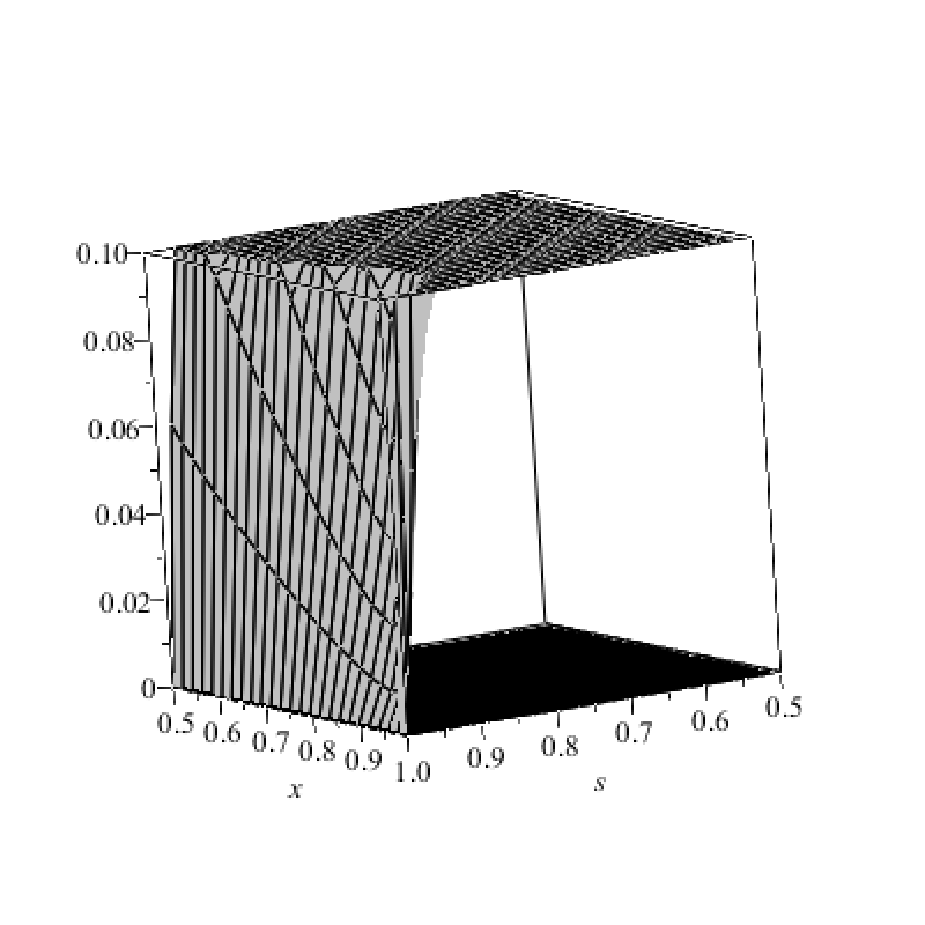
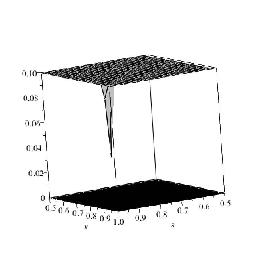
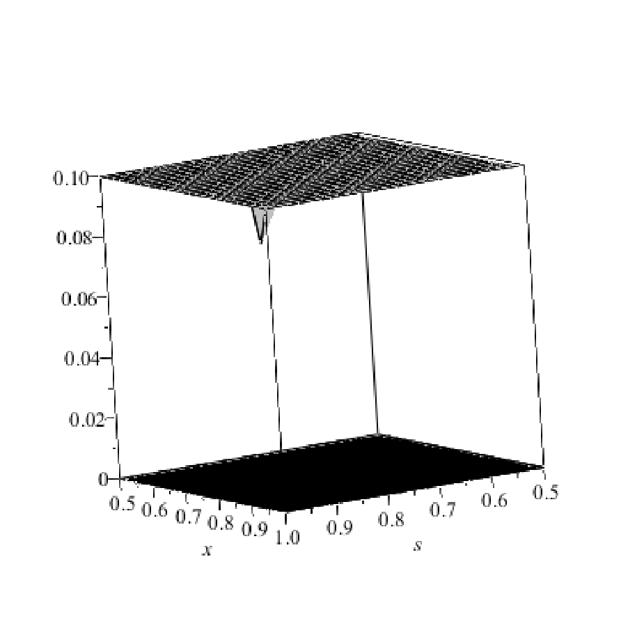
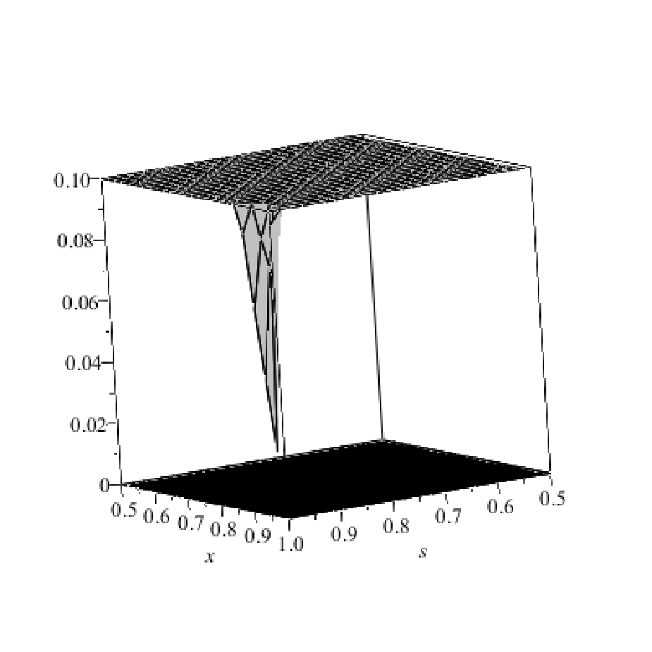
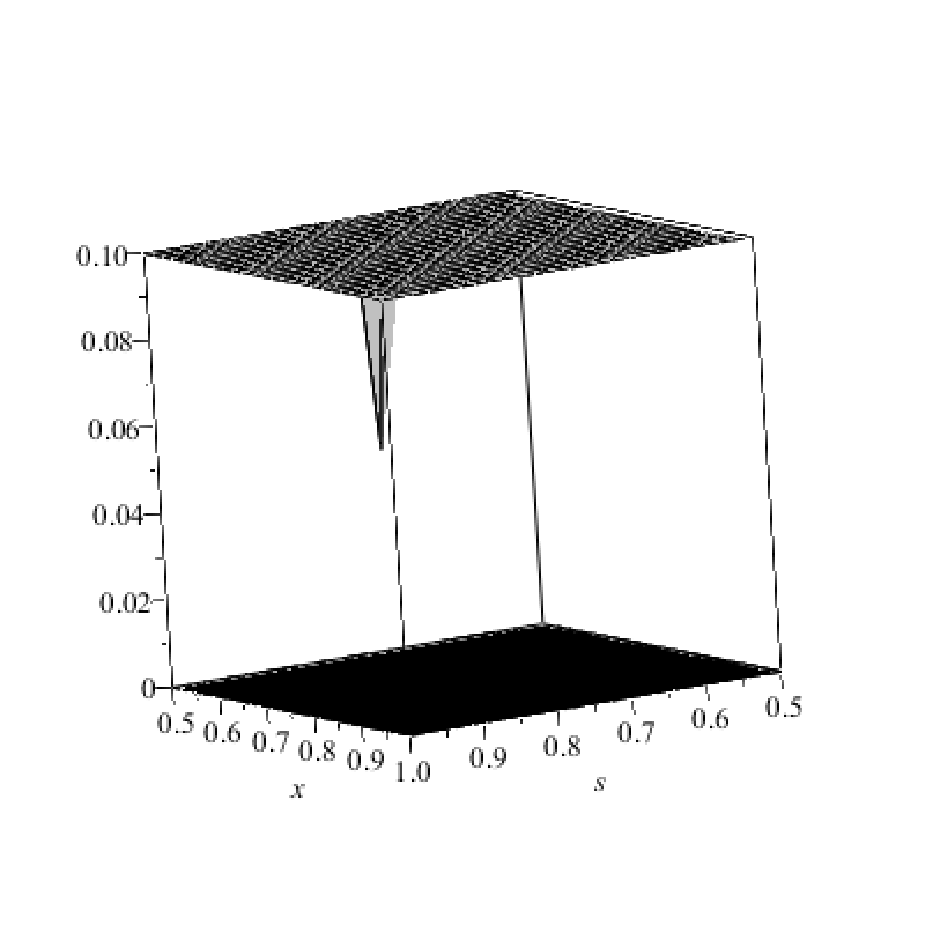
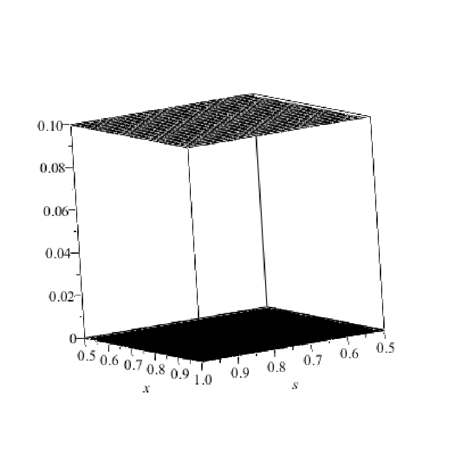
In Figure 4 we present the plots of the left-hand side of (5.6) for $n=2,\ldots,11$ , where this is indeed positive.

Remark 5.1.

By avoiding estimate (5.5) and keeping the series expansion of the hypergeometric function, see (A.4), it is possible to see that also the case $n=12$ is actually covered by this approach. However, for larger $n$ this keeps failing, although there always are some ranges of $s$ where the left-hand side of (5.4) stays positive. Finally, let us mention that for $n\geq 127$ , the left-hand side of (5.6) seems to be positive again. Indeed, again with the series expansion of the hypergeometric function, see (A.4), it holds for $n\geq 4$

\,{}_{2}F_{1}\bigg(\frac{n}{2}+1-2s,2-2s;\frac{n}{2}\Big|x^{2}\bigg)\leq\sum_{k=0}^{\infty}\frac{\Gamma(2-2s+k)}{\Gamma(2-2s)}\frac{x^{2k}}{k!}=\big(1-x^{2}\big)^{2s-2},

see (A.8). So that it remains to check

(5.7)

x^{4s-2-n}-\big(1-x^{2}\big)^{2s-2}+\frac{M(n,s)\Gamma\big(\frac{n}{2}+1\big)\,\Gamma(1-s)}{2\Gamma\big(\frac{n}{2}+2-s\big)}\big(1-x^{2}\big)^{s-2}\geq 0,

which seems to stay positive for $n\geq 127$ . See Figure 5. Note indeed that the left-hand side of (5.7) is greater than

x^{4s-2-n}-\big(1-x^{2}\big)^{2s-2}

which diverges to $+\infty$ as $n\uparrow\infty$ for $s,x\in(\frac{1}{2},1)$ .

Let us mention here that our strategy strongly relies also on estimate (B.1) and that a more precise estimate here could improve a lot the number of dimensions covered in our analysis.

Appendix A Special functions

For the reader’s convenience we list here the definitions and some properties about the special functions that we use.

A.1. The Gamma function

As usual, the Gamma function is defined by

\Gamma(z)=\int_{0}^{\infty}x^{z-1}e^{-x}\;dx,\qquad\text{for }z>0.

As it satisfies the recursive formula

\displaystyle\Gamma(z+1)=z\,\Gamma(z)

its definition can be extended using this formula to $z\in\mathbb{R}\setminus\{0,-1,-2,\ldots\}$ . The Gamma function satisfies in particular the duplication formula (see, e.g., [3]*equation 6.1.18)

(A.1)

\displaystyle\sqrt{\pi}\,\Gamma(2z)=2^{2z-1}\Gamma(z)\,\Gamma\Big(z+\frac{1}{2}\Big)\qquad\text{for }z>0.

Moreover, it holds (e.g., [3]*equation 6.1.17)

\displaystyle\Gamma(z)\Gamma(1-z)=\frac{\pi}{\sin(\pi z)}\qquad\text{for }z\in\mathbb{R}\setminus\mathbb{Z}.

Furthermore (e.g., [3]*equation 6.2.1),

(A.2)

\displaystyle\int_{0}^{1}t^{z-1}(1-t)^{w-1}\;dt=\int_{0}^{\infty}\frac{t^{z-1}}{(1+t)^{z+w}}\;dt=\frac{\Gamma(z)\,\Gamma(w)}{\Gamma(z+w)},\qquad z,w>0.

A.2. The hypergeometric function

We collect here some facts about the hypergeometric function $\,{}_{2}F_{1}$ . We suppose in all the following that $a,b,c,z\in\mathbb{R}$ with $c>b>0$ and $z\in[0,1)$ , although some formulas might hold in broader generality (we refer to [3]*Chapter 15).

Recall first the integral representation

(A.3)

\displaystyle\,{}_{2}F_{1}(a,b;c|z)=\frac{\Gamma(c)}{\Gamma(b)\,\Gamma(c-b)}\int_{0}^{1}t^{b-1}(1-t)^{c-b-1}(1-zt)^{-a}\;dt,

see [3]*equation 15.3.1, and the series expansion

(A.4)

\displaystyle\,{}_{2}F_{1}(a,b;c|z)=\frac{\Gamma(c)}{\Gamma(a)\Gamma(b)}\sum_{k=0}^{\infty}\frac{\Gamma(a+k)\Gamma(b+k)}{\Gamma(c+k)}\frac{z^{k}}{k!},

see [3]*equation 15.1.1.

In particular one can consider $-a\in\mathbb{N}\cup\{0\}$ , in which case one has that $\,{}_{2}F_{1}$ reduces to a polynomial of degree $-a$ . For example:

(A.5)		$\displaystyle\,{}_{2}F_{1}(0,b;c\|z)$	$\displaystyle=1,$
(A.6)		$\displaystyle\,{}_{2}F_{1}(-1,b;c\|z)$	$\displaystyle=1-\frac{b}{c}\,z,$

see [3]*equation 15.4.1.

Among the many possible transformations, the following one is important to our purposes:

(A.7)

\displaystyle\,{}_{2}F_{1}(a,b;c|z)=(1-z)^{c-a-b}\,{}_{2}F_{1}(c-a,c-b;c|z).

Indeed, (A.7) alongside (A.5) and (A.6) respectively, bears the following identities (corresponding to the particular cases $c=a$ and $c=a-1$ respectively):

(A.8)		$\displaystyle\,{}_{2}F_{1}(a,b;a\|z)$	$\displaystyle=(1-z)^{-b}$	$\displaystyle\text{if }a>b>0,$
(A.9)		$\displaystyle\,{}_{2}F_{1}(a,b;a-1\|z)$	$\displaystyle=(1-z)^{-b-1}\Big(1-\frac{a-b-1}{a-1}\,z\Big)$	$\displaystyle\text{if }a-1>b>0.$

Finally, according to [3]*formula 15.3.17,

(A.10)

\displaystyle\,{}_{2}F_{1}(a,b;2b|z)=2^{2a}\big(1+\sqrt{1-z}\big)^{-2a}\,{}_{2}F_{1}\bigg(a,a-b+\frac{1}{2};b+\frac{1}{2}\Big|\Big(\frac{1-\sqrt{1-z}}{1+\sqrt{1+z}}\Big)^{2}\bigg).

Appendix B A bound on the first eigenvalue

Let $\lambda$ be the first eigenvalue of $(-\Delta)^{s}$ in $B_{1}$ . A direct bound in terms the first eigenvalue $\lambda_{1}$ of the classical Dirichlet Laplacian $-\Delta$ on the same ball is given by

\lambda\leq\big(\lambda_{1}\big)^{s},

see [16]*Theorem 1.1 or, also, [9, 15]. To have a more explicit estimate—which turns out to be a better one for $s$ away from $1$ and $n=1$ —recall that the function $u_{1}\in C^{s}(\mathbb{R}^{n})$ , $u_{1}(x)=\kappa_{n,s}(1-|x|^{2})^{s}_{+}$ , where

\kappa_{n,s}=\frac{\Gamma(n/2)4^{-s}}{\Gamma(1+s)\Gamma(s+\frac{n}{2})},

satisfies $(-\Delta)^{s}u_{1}=1$ in $B_{1}$ . In particular, we have

\lambda=\min_{\begin{subarray}{c}u\in{\mathcal{H}}^{s}_{0}(B_{1})\\ u\neq 0\end{subarray}}\frac{[u]^{2}_{s}}{\|u\|_{L^{2}(B_{1})}^{2}}\leq\frac{[u_{1}]^{2}_{s}}{\|u_{1}\|_{L^{2}(B_{1})}^{2}}.

Here,

	$\displaystyle[u_{1}]^{2}_{s}$	$\displaystyle=\int_{B_{1}}u_{1}(x)\;dx=\kappa_{n,s}\frac{2\pi^{n/2}}{\Gamma(\frac{n}{2})}\int_{0}^{1}(1-r^{2})^{s}\,r^{n-1}\;dr$
		$\displaystyle=\kappa_{n,s}\frac{\pi^{n/2}}{\Gamma(\frac{n}{2})}\int_{0}^{1}(1-t)^{s}\,t^{\frac{n}{2}-1}\;dt=\kappa_{n,s}\pi^{n/2}\frac{\Gamma(1+s)}{\Gamma(1+s+\frac{n}{2})},$
	$\displaystyle\\|\tau\\|_{L^{2}(B_{1})}^{2}$	$\displaystyle=\kappa_{n,s}^{2}\frac{2\pi^{n/2}}{\Gamma(\frac{n}{2})}\int_{0}^{1}(1-r^{2})^{2s}\,r^{n-1}\;dr=\kappa_{n,s}^{2}\frac{\pi^{n/2}}{\Gamma(\frac{n}{2})}\int_{0}^{1}(1-t)^{2s}\,t^{\frac{n}{2}-1}\ dt$
		$\displaystyle=\kappa_{n,s}^{2}\pi^{n/2}\frac{\Gamma(1+2s)}{\Gamma(1+2s+\frac{n}{2})},$

where we used (A.2) twice. Thus,

(B.1)

\lambda\leq\frac{1}{\kappa_{n,s}}\frac{\Gamma(1+s)\Gamma(1+2s+\frac{n}{2})}{\Gamma(1+2s)\Gamma(1+s+\frac{n}{2})}=\frac{4^{s}\Gamma(1+s)^{2}\,\Gamma(1+2s+\frac{n}{2})}{(s+\frac{n}{2})\,\Gamma(\frac{n}{2})\,\Gamma(1+2s)}=\Lambda(n,s).

In the particular case $n=1$ , we have with the properties of the Gamma function (see Appendix A, in particular (A.1))

(B.2)

\displaystyle\lambda\leq\frac{4^{s}\Gamma(1+s)^{2}\,\Gamma(\frac{3}{2}+2s)}{(\frac{1}{2}+s)\,\Gamma(\frac{1}{2})\,\Gamma(1+2s)}=\frac{s4^{s}\Gamma(s)^{2}\,\Gamma(\frac{3}{2}+2s)}{\sqrt{\pi}(1+2s)\,\Gamma(2s)}=\frac{2s\Gamma(s)\,\Gamma(\frac{3}{2}+2s)}{(1+2s)\,\Gamma(\frac{1}{2}+s)}=\frac{\Gamma(1+s)\,\Gamma(\frac{3}{2}+2s)}{\Gamma(\frac{3}{2}+s)}.

Related results in this direction are contained in Dyda, Kuznetsov, and Kwaśnicki [11].

Appendix C On the shape of some $s$ -harmonic functions

We discuss here some features of $s$ -harmonic functions in $B_{1}$ associated with particular data in $B_{1}^{c}$ . Specifically, we assume

(C.1)		$\displaystyle g:(1,\infty)\to\mathbb{R}\quad\text{is a non-increasing function,}$
(C.2)		$\displaystyle\int_{\mathbb{R}^{n}\setminus B_{1}}\frac{\|g(y)\|}{1+{\|y\|}^{n+2s}}\;dy<\infty.$

We denote by

(C.3)

\displaystyle b_{t}=\sup\{y\in(1,\infty):g(y)>t\}\quad\text{for }t\in(-\infty,\overline{g}),\qquad\overline{g}=\lim_{y\downarrow 1}g(y).

Let $h:\mathbb{R}^{n}\to\mathbb{R}$ be the $s$ -harmonic extension of $y\to g(|y|)$ in $B_{1}$ , namely

(C.4)

\displaystyle h(x)=\int_{B_{1}^{c}}P_{s}(x,y)\,g(|y|)\;dy=\gamma_{n,s}\int_{B_{1}^{c}}\bigg(\frac{1-|x|^{2}}{|y|^{2}-1}\bigg)^{s}\frac{g(|y|)}{{|y-x|}^{n}}\;dy,\qquad\text{for }x\in B_{1}.

Proposition C.1.

Assume (C.1), (C.2), and that $g$ is non-negative. The function $h$ defined as in (C.4) is radial, radially increasing, and subharmonic in $B_{1}$ .

Proof.

Starting from the representation formula (C.4), we write

\displaystyle h(x)=\gamma_{n,s}\big(1-|x|^{2}\big)^{s}\int_{1}^{\infty}\frac{\rho^{n-1}\,g(\rho)}{\big(\rho^{2}-1\big)^{s}}\int_{\partial B_{1}}\frac{d\theta}{\big|\rho\theta-x\big|^{n}}\;d\rho

and, in view of Lemma 2.4, it holds for $x\in B_{1}$ and $\rho>1$

	$\displaystyle\int_{\partial B_{1}}\frac{d\theta}{\big\|\rho\theta-x\big\|^{n}}$	$\displaystyle=\frac{2\pi^{\frac{n-1}{2}}}{\Gamma(\frac{n-1}{2})}\int_{-1}^{1}\frac{(1-t^{2})^{\frac{n-3}{2}}}{(\rho^{2}+\|x\|^{2}-2\rho\|x\|t)^{\frac{n}{2}}}\;dt$
		$\displaystyle=\frac{2^{n-1}\pi^{\frac{n-1}{2}}}{\Gamma(\frac{n-1}{2})}\int_{0}^{1}\frac{\tau^{\frac{n-3}{2}}{(1-\tau)}^{\frac{n-3}{2}}}{\big((\rho+\|x\|)^{2}-4\rho\|x\|\tau\big)^{\frac{n}{2}}}\;d\tau$
		$\displaystyle=\frac{2^{n-1}\pi^{\frac{n-1}{2}}}{\Gamma(\frac{n-1}{2})}\frac{\Gamma(\frac{n-1}{2})}{\Gamma(n-1)}\big(\rho+\|x\|\big)^{-n}\,{}_{2}F_{1}\bigg(\frac{n}{2},\frac{n-1}{2};n-1\Big\|\frac{4\rho\|x\|}{(\rho+\|x\|)^{2}}\bigg)$
		$\displaystyle=\frac{2^{n-1}\pi^{\frac{n-1}{2}}}{}\frac{\Gamma(\frac{n-1}{2})}{\Gamma(n-1)}\rho^{-n}\,{}_{2}F_{1}\bigg(\frac{n}{2},1;\frac{n}{2}\Big\|\frac{\|x\|^{2}}{\rho^{2}}\bigg)$
		$\displaystyle=2^{n-1}\pi^{\frac{n-1}{2}}\frac{\Gamma(\frac{n-1}{2})}{\Gamma(n-1)}\frac{\rho^{2-n}}{\rho^{2}-\|x\|^{2}}$

where we have used (A.3), (A.10), and (A.8) in this order. Using the layer-cake representation for $g$

\displaystyle g(\rho)=\int_{0}^{\overline{g}}\mathbf{1}_{(1,b_{t})}(\rho)\;dt,\qquad\rho>1,

with $b_{t}$ and $\overline{g}$ defined as in (C.3), we write for $x\in B_{1}$

	$\displaystyle h(x)$	$\displaystyle=\gamma_{1,s}\big(1-\|x\|^{2}\big)^{s}\int_{1}^{\infty}\frac{2\rho\,g(\rho)}{\big(\rho^{2}-1\big)^{s}(\rho^{2}-\|x\|^{2})}\;d\rho$
		$\displaystyle=\gamma_{1,s}\big(1-\|x\|^{2}\big)^{s}\int_{0}^{\overline{g}}\int_{1}^{b_{t}}\frac{2\rho}{\big(\rho^{2}-1\big)^{s}(\rho^{2}-\|x\|^{2})}\;dy\;dt$

where, for any $b\geq 1$ ,

\int_{1}^{b}\frac{2\rho}{\big(\rho^{2}-1\big)^{s}(\rho^{2}-|x|^{2})}\;d\rho=\int_{1}^{b^{2}}\frac{dz}{{(z-1)}^{s}(z-|x|^{2})}=\int_{0}^{b^{2}-1}\frac{dz}{z^{s}(z+1-|x|^{2})}=\\ =\big(1-|x|^{2}\big)^{-s}\int_{0}^{\frac{b^{2}-1}{1-|x|^{2}}}\frac{dw}{w^{s}(w+1)}=\big(1-|x|^{2}\big)^{-s}\int_{\frac{1-|x|^{2}}{b^{2}-1}}^{\infty}\frac{v^{s-1}}{v+1}\;dv.

Therefore

\displaystyle h(x)=\gamma_{1,s}\int_{0}^{\overline{g}}\int_{\frac{1-|x|^{2}}{b_{t}^{2}-1}}^{\infty}\frac{v^{s-1}}{v+1}\;dv\;dt\qquad\text{for }x\in B_{1}.

As a consequence, for any $x\in B_{1}$ ,

\displaystyle\nabla h(x)

\displaystyle=-\gamma_{1,s}\int_{0}^{\overline{g}}\bigg(\frac{1-|x|^{2}}{b_{t}^{2}-1}\bigg)^{s-1}\frac{1}{\frac{1-|x|^{2}}{b_{t}^{2}-1}+1}\,\frac{-2x}{b_{t}^{2}-1}\;dt=2\gamma_{1,s}\,x\big(1-|x|^{2}\big)^{s-1}\int_{0}^{\overline{g}}\frac{\big(b_{t}^{2}-1\big)^{1-s}}{b_{t}^{2}-|x|^{2}}\;dt.

This proves the radial monotonicity. Moreover, for any $x\in B_{1}$ ,

	$\displaystyle-\Delta h(x)$	$\displaystyle=-2\gamma_{1,s}\;\mathrm{div}\bigg(x\big(1-\|x\|^{2}\big)^{s-1}\int_{0}^{\overline{g}}\frac{\big(b_{t}^{2}-1\big)^{1-s}}{b_{t}^{2}-\|x\|^{2}}\;dt\bigg)$
		$\displaystyle=-2n\gamma_{1,s}\,\big(1-\|x\|^{2}\big)^{s-1}\int_{0}^{\overline{g}}\frac{\big(b_{t}^{2}-1\big)^{1-s}}{b_{t}^{2}-\|x\|^{2}}\;dt-4(1-s)\gamma_{1,s}\,\|x\|^{2}\big(1-\|x\|^{2}\big)^{s-2}\int_{0}^{\overline{g}}\frac{\big(b_{t}^{2}-1\big)^{1-s}}{b_{t}^{2}-\|x\|^{2}}\;dt$
		$\displaystyle\qquad-4\gamma_{1,s}\,\|x\|^{2}\big(1-\|x\|^{2}\big)^{s-1}\int_{0}^{\overline{g}}\frac{\big(b_{t}^{2}-1\big)^{1-s}}{\big(b_{t}^{2}-\|x\|^{2}\big)^{2}}\;dt$

is (strictly) negative for $x\in B_{1}$ . ∎

Remark C.2.

Analogue calculations can be performed when $g$ is non-negative and non-decreasing instead. This would lead to a radial, radially decreasing, and super-harmonic $s$ -harmonic extension.

Remark C.3.

The non-negativity assumption in Proposition C.1 can be dropped: if we split $g=g^{+}-g^{-}$ we can directly apply Proposition C.1 to $g^{+}$ and Remark C.2 to $g^{-}$ .

References

[1] N. Abatangelo and E. Valdinoci (2019) Getting acquainted with the fractional laplacian. pp. 1–105. Cited by: §1.
[2] N. Abatangelo (2015) Large $s$ -harmonic functions and boundary blow-up solutions for the fractional laplacian. Discrete Contin. Dyn. Syst. 35 (12), pp. 5555–5607. Cited by: §2.1.
[3] M. Abramowitz and I.A. Stegun (1964) Handbook of mathematical functions with formulas, graphs, and mathematical tables. National Bureau of Standards Applied Mathematics Series, Vol. 55, For sale by the Superintendent of Documents, U.S. Government Printing Office, Washington, D.C.. Cited by: §A.1, §A.1, §A.1, §A.2, §A.2, §A.2, §A.2, §A.2.
[4] R. Bañuelos and D. DeBlassie (2015) On the first eigenfunction of the symmetric stable process in a bounded lipschitz domain. Potential Anal. 42 (2), pp. 573–583. Cited by: §1.
[5] R. Bañuelos, T. Kulczycki, and P.J. Méndez-Hernández (2006) On the shape of the ground state eigenfunction for stable processes. Potential Anal. 24 (3), pp. 205–221. Cited by: §1, §1, item 1.
[6] R. Bañuelos and T. Kulczycki (2004) The cauchy process and the steklov problem. J. Funct. Anal. 211 (2), pp. 355–423. Cited by: §1.
[7] C. Bucur and E. Valdinoci (2016) Nonlocal diffusion and applications. Lecture Notes of the Unione Matematica Italiana, Vol. 20, Springer, [Cham]; Unione Matematica Italiana, Bologna. Cited by: §1.
[8] C. Bucur (2016) Some observations on the green function for the ball in the fractional laplace framework. Commun. Pure Appl. Anal. 15 (2), pp. 657–699. Cited by: §2.1.
[9] Z.-Q. Chen and R. Song (2005) Two-sided eigenvalue estimates for subordinate processes in domains. J. Funct. Anal. 226 (1), pp. 90–113. Cited by: Appendix B.
[10] E. Di Nezza, G. Palatucci, and E. Valdinoci (2012) Hitchhiker’s guide to the fractional sobolev spaces. Bull. Sci. Math. 136 (5), pp. 521–573. Cited by: §1.
[11] B. Dyda, A. Kuznetsov, and M. Kwaśnicki (2017) Eigenvalues of the fractional laplace operator in the unit ball. J. Lond. Math. Soc. (2) 95 (2), pp. 500–518. Cited by: Appendix B.
[12] N. Garofalo (2019) Fractional thoughts. pp. 1–135. Cited by: §1.
[13] M. Kaßmann and L. Silvestre (2014) On the superharmonicity of the first eigenfunction of the fractional laplacian for certain exponents. Note: Available at https://www.math.uchicago.edu/~luis/preprints/cfe.pdf Cited by: §1.
[14] N.S. Landkof (1972) Foundations of modern potential theory. Die Grundlehren der mathematischen Wissenschaften, Band 180, Springer-Verlag, New York-Heidelberg. Note: Translated from the Russian by A. P. Doohovskoy Cited by: §2.1.
[15] R. Musina and A. I. Nazarov (2014) On fractional laplacians. Comm. Partial Differential Equations 39 (9), pp. 1780–1790. Cited by: Appendix B.
[16] R. Servadei and E. Valdinoci (2014) On the spectrum of two different fractional operators. Proc. Roy. Soc. Edinburgh Sect. A 144 (4), pp. 831–855. Cited by: Appendix B.
[17] L. Silvestre (2007) Regularity of the obstacle problem for a fractional power of the laplace operator. Comm. Pure Appl. Math. 60 (1), pp. 67–112. Cited by: §2.1.

	$\displaystyle\int_{B_{1}^{c}}P_{s}(y,z)\,J_{\tau}(x;z)\;dz$	$\displaystyle=\frac{\Gamma(\frac{n}{2})}{\pi^{\frac{n}{2}}\Gamma(s)\Gamma(1-s)}\int_{B_{1}^{c}}\frac{(1-\|y\|^{2})^{s}}{(\|z\|^{2}-1)^{s}\|y-z\|^{n}}\,J_{\tau}(\|x\|e_{1};\|z\|e_{1})\;dz$
		$\displaystyle=\frac{\Gamma(\frac{n}{2})}{\pi^{\frac{n}{2}}\Gamma(s)\Gamma(1-s)}\int_{B_{1}^{c}}\frac{(1-\|y\|^{2})^{s}}{(\|z\|^{2}-1)^{s}\big(\|y\|^{2}-2y\cdot z+\|z\|^{2}\big)^{\frac{n}{2}}}\,J_{\tau}(\|x\|e_{1};\|z\|e_{1})\;dz$
		$\displaystyle=\frac{\Gamma(\frac{n}{2})}{\pi^{\frac{n}{2}}\Gamma(s)\Gamma(1-s)}\int_{B_{1}^{c}}\frac{(1-\|y\|^{2})^{s}}{(\|v\|^{2}-1)^{s}\big(\|y\|^{2}-2\|y\|v_{1}+\|v\|^{2}\big)^{\frac{n}{2}}}\,J_{\tau}(\|x\|e_{1};\|v\|e_{1})\;dv$
		$\displaystyle=\frac{\Gamma(\frac{n}{2})}{\pi^{\frac{n}{2}}\Gamma(s)\Gamma(1-s)}\int_{B_{1}^{c}}\frac{(1-\|y\|^{2})^{s}}{(\|v\|^{2}-1)^{s}\big\|\|y\|e_{1}-v\big\|^{n}}\,J_{\tau}(\|x\|e_{1};\|v\|e_{1})\;dv$
		$\displaystyle=\int_{B_{1}^{c}}P_{s}(\|y\|e_{1},v)\,J_{\tau}(\|x\|e_{1};v)\;dv.$

	$\displaystyle\Big(\frac{1}{2},1\Big)\times\Big(\frac{1}{2},1\Big)$	$\displaystyle\longrightarrow\mathbb{R}$
	$\displaystyle(s,x)$	$\displaystyle\longmapsto\min\Bigg\{\frac{1}{10},x^{4s-2-n}-\,{}_{2}F_{1}\bigg(\frac{n}{2}+1-2s,2-2s;\frac{n}{2}\Big\|x^{2}\bigg)$
		$\displaystyle\qquad\qquad\qquad+\frac{M(n,s)\Gamma\big(\frac{n}{2}+1\big)\,\Gamma(1-s)}{2\Gamma\big(\frac{n}{2}+2-s\big)}\big(1-x^{2}\big)^{s-2}\Bigg\}$

	$\displaystyle\int_{\partial B_{1}}\frac{d\theta}{\big\|\rho\theta-x\big\|^{n}}$	$\displaystyle=\frac{2\pi^{\frac{n-1}{2}}}{\Gamma(\frac{n-1}{2})}\int_{-1}^{1}\frac{(1-t^{2})^{\frac{n-3}{2}}}{(\rho^{2}+\|x\|^{2}-2\rho\|x\|t)^{\frac{n}{2}}}\;dt$
		$\displaystyle=\frac{2^{n-1}\pi^{\frac{n-1}{2}}}{\Gamma(\frac{n-1}{2})}\int_{0}^{1}\frac{\tau^{\frac{n-3}{2}}{(1-\tau)}^{\frac{n-3}{2}}}{\big((\rho+\|x\|)^{2}-4\rho\|x\|\tau\big)^{\frac{n}{2}}}\;d\tau$
		$\displaystyle=\frac{2^{n-1}\pi^{\frac{n-1}{2}}}{\Gamma(\frac{n-1}{2})}\frac{\Gamma(\frac{n-1}{2})}{\Gamma(n-1)}\big(\rho+\|x\|\big)^{-n}\,{}_{2}F_{1}\bigg(\frac{n}{2},\frac{n-1}{2};n-1\Big\|\frac{4\rho\|x\|}{(\rho+\|x\|)^{2}}\bigg)$
		$\displaystyle=\frac{2^{n-1}\pi^{\frac{n-1}{2}}}{}\frac{\Gamma(\frac{n-1}{2})}{\Gamma(n-1)}\rho^{-n}\,{}_{2}F_{1}\bigg(\frac{n}{2},1;\frac{n}{2}\Big\|\frac{\|x\|^{2}}{\rho^{2}}\bigg)$
		$\displaystyle=2^{n-1}\pi^{\frac{n-1}{2}}\frac{\Gamma(\frac{n-1}{2})}{\Gamma(n-1)}\frac{\rho^{2-n}}{\rho^{2}-\|x\|^{2}}$

	$\displaystyle-\Delta h(x)$	$\displaystyle=-2\gamma_{1,s}\;\mathrm{div}\bigg(x\big(1-\|x\|^{2}\big)^{s-1}\int_{0}^{\overline{g}}\frac{\big(b_{t}^{2}-1\big)^{1-s}}{b_{t}^{2}-\|x\|^{2}}\;dt\bigg)$
		$\displaystyle=-2n\gamma_{1,s}\,\big(1-\|x\|^{2}\big)^{s-1}\int_{0}^{\overline{g}}\frac{\big(b_{t}^{2}-1\big)^{1-s}}{b_{t}^{2}-\|x\|^{2}}\;dt-4(1-s)\gamma_{1,s}\,\|x\|^{2}\big(1-\|x\|^{2}\big)^{s-2}\int_{0}^{\overline{g}}\frac{\big(b_{t}^{2}-1\big)^{1-s}}{b_{t}^{2}-\|x\|^{2}}\;dt$
		$\displaystyle\qquad-4\gamma_{1,s}\,\|x\|^{2}\big(1-\|x\|^{2}\big)^{s-1}\int_{0}^{\overline{g}}\frac{\big(b_{t}^{2}-1\big)^{1-s}}{\big(b_{t}^{2}-\|x\|^{2}\big)^{2}}\;dt$

On the shape of the first fractional eigenfunctionThanks: MSC2020: Primary: 47A75, 35B99, 35P05; Secondary: 47G20, 35R11. Thanks: Acknowledgements: The first author has been partially supported by the Alexander von Humboldt Foundation.

Abstract.

1. Introduction

Theorem 1.1.

Theorem 1.2.

1.1. Notations

2. Set-up of the proof of Theorems 1.1 and 1.2

2.1. Representation of the Laplacian of the eigenfunction

Lemma 2.1.

Proof.

Proposition 2.2.

Proof.

2.2. Reformulation of (2.8)

Lemma 2.3.

Proof.

Lemma 2.4.

Proof.

Lemma 2.5.

Proof.

Lemma 2.6.

Proof.

Lemma 2.7.

Remark 2.8.

Proof of Lemma 2.7.

Lemma 2.9.

Proof.

3. The one-dimensional case: s=3/4s=3/4

4. The general one-dimensional case

5. The higher-dimensional case

Remark 5.1.

Appendix A Special functions

A.1. The Gamma function

A.2. The hypergeometric function

Appendix B A bound on the first eigenvalue

Appendix C On the shape of some ss-harmonic functions

Proposition C.1.

Proof.

Remark C.2.

Remark C.3.

References

3. The one-dimensional case: $s=3/4$

Appendix C On the shape of some $s$ -harmonic functions