Graph polynomial for colored embedded graphs: a topological approach

Somnath Basu Address: Department of Mathematics & Statistics, Indian Institute of Science Education & Research, Mohanpur 741246, West Bengal, India Email address: somnath.basu@iiserkol.ac.in , Dhruv Bhasin Address: Department of Mathematical Sciences, Indian Institute of Science Education and Research Pune, Maharashtra - 411008, India Email address: bhasin.dhruv@students.iiserpune.ac.in , Siddhartha Lal Address: Department of Physical Sciences, Indian Institute of Science Education & Research, Mohanpur 741246, West Bengal, India Email address: slal@iiserkol.ac.in and Siddhartha Patra Address: Department of Physical Sciences, Indian Institute of Science Education & Research, Mohanpur 741246, West Bengal, India Email address: sp14ip022@iiserkol.ac.in

Abstract.

We study finite graphs embedded in oriented surfaces by associating a polynomial to it. The tools used in developing a theory of such graph polynomials are algebraic topological while the polynomial itself is inspired from ideas arising in physics. We also analyze a variant of these polynomials for colored embedded graphs. This is used to describe the change in the polynomial under basic graph theoretic operations. We conclude with several applications of this polynomial including detection of certain classes of graphs and the connection of this polynomial with topological entanglement entropy.

Key words and phrases:

Graph polynomial, embedded graphs, vertex colored graphs, topological entanglement entropy

2020 Mathematics Subject Classification

Primary 05C31, 05C90, Secondary 57K20.

1. Introduction

In algebraic graph theory, invariants of graphs taking values in polynomials are natural objects of interest. The importance stems from its applicability and the underlying power of algebra in efficiently packaging information. Such graph polynomials include the characteristic polynomial and chromatic polynomial. All of the commonly known polynomial invariants (including the celebrated Tutte polynomial) are invariants of the graph and need not admit natural generalizations to embedded graphs. We propose a new graph polynomial $\beta_{(\Gamma,\sigma)}$ (Definition 2.5), heavily borrowing from ideas arising from a recent study of topological entanglement entropy by us [34]. Given a graph $\Gamma$ embedded in an oriented surface $\Sigma$ , we define a polynomial built out of signed counts of the number of faces of all induced subgraphs. We make use of algebraic topology, whenever needed, to develop a theory of such polynomials.
Graph polynomials have been traditionally used to study properties of graphs, including adjacency (characteristic polynomial), coloring (Birkhoff’s chromatic polynomial [5]), Euler tours, rank polynomial [12] and more. Apart from the standard graph polynomials, there is the Ihara zeta function [14] which is useful in the study of free groups, spectral graph theory and symbolic dynamics. The famous Tutte polynomial [47, 48, 6] encodes information about connectivity of induced subgraphs. It is equivalent to the Whitney rank generating function, related to the Jones polynomial (in knot theory), as well as connected to several computational problems in theoretical computer science. Historically, there have been connections between works in physics and graph polynomials. As as example, after Potts work [38] on partition function of certain models in statistical mechanics in 1952, Fortuin and Kasteleyn [11] found connections between Tutte polynomial and their work on random cluster model, a generalisation of the Potts model. In their work in 2010, Chang and Shrock [7] had defined a polynomial $Ph(G,q,w)$ , which generalizes the chromatic polynomial $P(G,q)$ . Their aim was to study the statistical mechanics of the Potts antiferromagnet in a magnetic field as well as use these weighted graph coloring polynomials to solve problems that have physical applications. A recent study [34] of the entanglement entropy of a topologically ordered state of quantum matter [52, 53, 54] sheds light on the connection between multipartite quantum information measure and questions in graph theory.
The complexity and subtlety of the nature of graph polynomials we are defining (and analyzing) stems from the fact that a graph can have several inequivalent embeddings inside the same surface. This may generate different $\beta$ for the same graph. On the one hand, the theory yields results requiring very few hypotheses when we are dealing with planar graphs. On the other hand, since any finite graph can be embedded in surfaces of high enough genus, no finite graphs are excluded from the ambit of our approach. In fact, for any vertex coloring $\mathfrak{c}$ (not necessarily a proper vertex coloring) of an embedded graph, we have a generalization of our graph polynomial $\beta_{(\Gamma,\sigma,\mathfrak{c})}$ (Definition 4.3). This reduces to Definition 2.5 when each vertex has a distinct color.
The colored graph polynomial $\beta_{(\Gamma,\sigma,\mathfrak{c})}$ is essential in studying how the graph polynomial $\beta_{(\Gamma,\sigma)}$ changes when we do an edge contraction or an edge subdivision. We also analyze the effect of adding a self-loop as well as adding an edge between vertices that already have an edge (we call this a similar adjacency). This requires a choice of an extension of the embedding. Moreover, it becomes abundantly clear with use that the value of the polynomial at $x=-1$ , i.e., $\beta_{(\Gamma,\sigma)}(-1)$ plays an important role. We call this number the total island count of the embedded graph $(\Gamma,\sigma)$ . If $\Gamma$ has $N$ vertices, then from the perspective of physics, the total island count is, for instance, related to the $N$ -partite information among $N$ subsystems in a topologically ordered ground state [52, 53, 54] . We map a collection of $N$ subsystems to a graph $\Gamma$ by representing each subsystem with a vertex and the connectivity between two subsystems by an edge connecting the two corresponding vertices. Thus, holes in the subsystem are represented by chordless cycles in the graph.
There are several results we prove about $\beta$ which indicate the non-trivial nature as well as potential utility of the polynomial invariant. The first main result, which is actually a combination of Theorem 2.13, Theorem 5.1, Theorem 5.3 and Theorem 5.4, is the following.

Theorem A.

The $\beta$ polynomial has the following properties:
(a) it detects planar trees;
(b) it detects planar connected graphs built out of trees by adding self-loops and similar adjacencies;
(c) it detects planar cycle graphs.

For non-planar graphs, the analogue of (a) is that $\beta$ gives the same polynomial for a tree and the same tree with self-loops and similar adjacencies (see Definition 3.3). Thus, $\beta$ can detect trees embedded in higher genus surfaces modulo self-loops and similar adjacencies. For non-planar graphs, the analogue of (c) is that $\beta$ gives the same polynomial for a cycle graph and the same graph with self-loops and similar adjacencies. Thus, $\beta$ can detect cycle graphs embedded in higher genus surfaces modulo self-loops and similar adjacencies. Properties (a) and (c) for non-planar graphs, as explained in the preceding lines, are perhaps the best possible since the domain of embedding, being no longer planar, has non-trivial topology.
Apart from the main results, we have several applications (Proposition 5.6, discussion in §5.3 and §5.4) which have been collected in the following.

Theorem B.

The total island count $\beta(-1)$ satisfies the following properties:
(a) it vanishes for tree-cycle graphs;
(b) it vanishes for a wedge sum of graphs;
(c) the vanishing of the multipartite information measure for a planar collection of subsystems is equivalent to the vanishing of $\beta(-1)$ for the associated graph;
(d) the alternating sum of $\beta(-1)$ over all subgraphs, on at least $3$ vertices, of a given planar graph $\Gamma$ is $\chi-2f$ , where $f$ is the number of faces.

We define tree-cycle graphs (see Definition 5.5) as graphs built out of trees through one of two operations. Through a judicious use of the colored $\beta$ polynomial, we may reduce a large class of planar graphs to tree-cycle graphs without changing $\beta(-1)$ . We view (d), which can be generalized to certain non-planar graphs, as the emergence of the Euler characteristic (which is a global topological invariant). This has been shown by some of us recently [34] via computations of multipartite information on a plane, which capture the Topological Entanglement Entropy (TEE) [19, 23] of a topologically ordered phases of quantum matter [52, 53, 54]. We also note that a recent work [46] has shown that the multipartite information between $D+1$ partitions of a $D$ -dimensional non-interacting Fermi gas is proportional to the Euler characteristic of the $D$ -dimensional Fermi volume.
The examples and discussions presented in §4.5 indicate that the graph polynomial approach we formulate is capable of tracking the changes in topology of the embedded graph upon carrying out certain transformations that are discussed in §4. As discussed there, this is of likely relevance to the study of dynamical transitions in non-linear dynamical systems [45, 4] and phase transitions in statistical mechanics within the Ginzburg-Landau-Wilson paradigm [17]. Our formalism is likely to be relevant to the paradigm of fermionic criticality, i.e., the Lifshitz phase transitions of systems of interacting fermions that involve changes in the topology of the Fermi volume [24, 50, 51, 28, 29, 26, 27, 32, 35, 31, 30, 33].
Graph theory has gradually become an essential part of computer science [8, 40, 25] as well as network analysis [1, 3, 9, 41] (see also [2] for a recent review on applications in physics). We firmly believe that the theory and results presented here will be useful to the community working on network analysis and applications of quantum information theory to quantum condensed matter physics (such as TEE), apart from its use within the graph theory community.

Organization of the paper. In §2, we define the $\beta$ polynomial, explore some of its basic properties in §2.1. We also compute this polynomial for trees and cycle graphs in §2.2. In §3 we analyze the change in $\beta$ under basic transformations - adding a self-loop (§3.1) and replicating an edge (§3.2). In §4 we introduce a colored variant of $\beta$ . This helps us in analyzing the change in $\beta$ under edge contraction (§4.2), edge subdivision (§4.3). In §4.4 the colored variant is used to compute $\beta$ for a graph which is a clean short-circuit (see Definition 4.18). In §4.5 we analyze, from several different points of view, a transformation that appears in a myriad of places within mathematics and physics. We observe that the $\beta$ polynomial detects the degeneration involved in the transformation. Finally, in §5, we give several applications of the theory presented here. This includes detection of trees and cycles (for planar graphs), evaluation of total island count for tree-cycle graphs, connections of $\beta$ polynomial to topological entanglement entropy and the recovery of Euler characteristic via signed total island counts of subgraphs.

Acknowledgments. The authors would like to thank Kaneenika Sinha, Moumanti Podder, Soumya Bhattacharya and Niranjan Balachandran for initial discussions on this topic. S. Basu would like to thank SERB for support through MATRICS grant MTR/2017/000807. D. Bhasin would like to acknowledge NBHM grant 0203/2/2021/RD-II/3033. S. Lal thanks the SERB, Govt. of India for funding through MATRICS grant MTR/2021/000141 and Core Research Grant CRG/2021/000852. S. Patra would like to thank CSIR and IISER Kolkata for funding through a research fellowship.

2. An invariant for finite graphs

A graph is typically denoted by $\Gamma=(V,E)$ , where $V:=V(\Gamma)$ is the set of vertices and $E:=E(\Gamma)$ is the set of edges. We shall consider graphs where multiple edges between vertices are allowed. In particular, we allow for self-loops as valid edges. Usually, such graphs are called multigraphs, but we will refer to these as graphs in what follows. Thus, $E$ is a multiset and not just a subset of $V\times V$ . If $\Gamma$ is a finite graph, i.e., both $V$ and $E$ are finite sets, then $v=|V|$ and $e=|E|$ will denote the number of vertices and edges, respectively. As we shall be dealing with induced subgraphs throughout this article, let us recall what these are. A subgraph $\Gamma^{\prime}$ with a vertex set $S$ is called induced if any edge in $\Gamma$ joining two vertices in $S$ is also in the subgraph. We will typically be dealing with non-trivial induced subgraphs, i.e., an induced subgraph where the vertex set is neither $\varnothing$ nor $V(\Gamma)$ . Note that a graph can be given a natural (quotient) topology by identifying edges with $[0,1]$ and subsequently identifying endpoints of intervals according to the adjacency relations in $\Gamma$ .
Let $\mathscr{F}(\Gamma)$ denote the collection of non-trivial induced subgraphs of $\Gamma$ . This is a disjoint union of $\mathscr{F}_{i}(\Gamma)$ , consisting of induced subgraphs of $\Gamma$ on $i$ vertices. A connected subgraph will be called an island. We shall be assigning certain integers to the data of a finite graph and an embedding of it inside a connected surface. Our analysis of these integers will be done via a generating polynomial method.

Definition 2.1 (Island boundary count).

Let $\sigma:\Gamma\hookrightarrow\Sigma$ be an embedding of $\Gamma$ in a connected surface $\Sigma$ . For any connected subgraph $\Gamma^{\prime}$ of $\Gamma$ , let $f_{\sigma}(\Gamma^{\prime})$ denote the number of path components of $\Sigma-\sigma(\Gamma^{\prime})$ . For a general subgraph $\Gamma^{\prime}$ with components (or islands) $\Gamma^{\prime}_{1},\ldots,\Gamma^{\prime}_{k}$ , we define

f_{\sigma}(\Gamma^{\prime}):=\sum_{i=1}^{k}f_{\sigma}(\Gamma^{\prime}_{i}).

Define the $i^{\textup{th}}$ island boundary count of $\Gamma$ with respect to the embedding $\sigma$ to be

\mathcal{D}_{i}(\Gamma,\sigma)=\sum_{\mathscr{F}_{i}}f_{\sigma}(\Gamma^{\prime}).

Note that $\mathcal{D}_{v(\Gamma)}(\Gamma,\sigma)$ , by extension of the definition, is the number of components of $\Sigma-\sigma(\Gamma)$ . We use the convention that $f_{\sigma}(\varnothing)=0$ .

Remark 2.2.

The notation $f$ is used to remind us of the fact that the number of path components of $\Sigma-\sigma(\Gamma^{\prime})$ is the number of faces, if we consider a triangulation of the surface by $\Gamma^{\prime}$ . For a planar connected graph $\Gamma$ , i.e., an embedded graph $\sigma:\Sigma\hookrightarrow S^{2}$ , the number of faces $f_{\sigma}(\Gamma)$ is the number of boundary components of a thickening of $\sigma(\Gamma)$ (figure 1). This explains the nomenclature in the definition.

Refer to caption — Figure 1. The term $\mathcal{D}_{v}(\Gamma)$ counts the number of boundary components, indicated by dashed blue curves, of a thickening of the edges.

Example 2.3 (Planar graphs).

For any connected graph $\Gamma$ which can be embedded in the plane (or, equivalently the $2$ -sphere), any two embeddings have the same number of faces, i.e., the number of path components in $S^{2}-\sigma(\Gamma)$ is independent of $\sigma$ . This is due to the famous Euler’s formula $v-e+f=2$ , which implies

(2.1)

f_{\sigma}(\Gamma)=2-v(\Gamma)+e(\Gamma).

Proposition 2.4.

Let $\Gamma$ be a finite graph such that any proper induced subgraph is a disjoint union of trees. Then for any embedding $\sigma:\Gamma\hookrightarrow\Sigma$ inside a connected surface,

\mathcal{D}_{i}(\Gamma,\sigma)=\sum_{\Gamma^{\prime}\in\mathscr{F}_{i}}H_{0}(\Gamma^{\prime}),

where $H_{0}(\Gamma^{\prime})$ denotes the rank of the zeroth homology¹¹ 1 It is also the number of connected components of $\Gamma^{\prime}$ . of the space $\Gamma^{\prime}$ (with $\mathbb{Z}$ coefficients).

It can be verified that $\Gamma$ as above is a disjoint union of trees. In this case, $\mathcal{D}_{i}(\Gamma,\sigma)$ counts the total number of islands formed out of all possible induced subgraphs of $\Gamma$ with $i$ number of vertices. This count was first used to measure the multi-partite information of a topologically ordered system [52, 18, 37] in theoretical condensed matter physics, where the physical attributes of a subgraph $\Gamma^{\prime}$ were dependent on the number of islands of a subgraph.

Proof.

Let $\Gamma^{\prime}$ be an induced subgraph of $\Gamma$ ; it will have components $\Gamma_{1},\ldots,\Gamma_{k}$ , all of which are trees. For a planar embedding $\sigma$ , using $0=1-v(\Gamma_{j})+e(\Gamma_{j})$ in conjunction with (2.1), we obtain

f_{\sigma}(\Gamma^{\prime})=\sum_{j=1}^{k}\big(2-v(\Gamma_{j})+e(\Gamma_{j})\big)=k=H_{0}(\Gamma^{\prime}).

For an embedding into an arbitrary surface $\Sigma$ , note that

f_{\sigma}(\Gamma^{\prime})=\sum_{j=1}^{k}f_{\sigma}(\Gamma_{j})=k

as the complement of any embedded tree is connected. The claim now follows from Definition 2.1 of $\mathcal{D}_{i}(\Gamma,\sigma)$ . ∎

Definition 2.5 (Signed island boundary polynomial).

For an embedded finite graph $(\Gamma,\sigma)$ , we define the island boundary polynomial to be

\bar{\beta}_{(\Gamma,\sigma)}(x):=\sum_{i=1}^{v-1}\mathcal{D}_{i}(\Gamma,\sigma)x^{i-1}.

The integer $\bar{\beta}(-1)$ will be called the signed island boundary count. The modified polynomial

{\beta}_{(\Gamma,\sigma)}(x):=\bar{\beta}_{(\Gamma,\sigma)}(x)+\mathcal{D}_{v}(\Gamma,\sigma)x^{v-1}

is defined as the total island boundary polynomial or the total island polynomial, in short. The integer ${\beta}(-1)$ is defined as the total signed island boundary count or the total island count, in short.

2.1. Basic properties & consequences

Let us consider the extreme case of a totally disconnected graph $D_{n}$ , on $n$ vertices. Since any two embeddings of $D_{n}$ in a connected surface are isotopic, we may drop the embedding in our count. The $i^{\textup{th}}$ island boundary count is given by ${n\choose i}i$ . It follows that

{\beta}_{D_{n}}(x)=n(1+x)^{n-1}.

In particular, the total island count is ${\beta}(D_{n})=0$ if $n>1$ . By computing a few examples (as shown in figure 2) we realize that the total island count is zero for a disjoint union of two (connected) graphs.

Figure 2. Graphs with two components

Proposition 2.6.

The total island count ${\beta}(-1)$ vanishes for a graph $(\Gamma,\sigma)$ which has at least $2$ components.

Proof.

Consider an embedded graph $(\Gamma,\sigma)$ , where $\Gamma$ can be written as the disjoint union of subgraphs $\Gamma_{1}$ and $\Gamma_{2}$ with $n_{1}$ and $n_{2}$ vertices respectively. The subgraphs $\Gamma_{i}$ need not be connected. Any subgraph $\Gamma^{\prime}$ can be decomposed as $\Gamma_{1}^{\prime}\sqcup\Gamma_{2}^{\prime}$ with $\Gamma_{j}^{\prime}=\Gamma_{j}\cap\Gamma^{\prime}$ . It follows that

f_{\sigma}(\Gamma^{\prime})=f_{\sigma}(\Gamma_{1}^{\prime})+f_{\sigma}(\Gamma_{2}^{\prime})

(2.2)	$\displaystyle{\beta}_{(\Gamma_{1}\sqcup\Gamma_{2},\sigma)}(x)$	$\displaystyle=$	$\displaystyle\sum_{j=1}^{n_{1}+n_{2}}x^{j-1}\sum_{\Gamma_{i}^{\prime}\subseteq\Gamma_{i},v(\Gamma_{1}^{\prime})+v(\Gamma_{2}^{\prime})=j}\big(f_{\sigma}(\Gamma_{1}^{\prime})+f_{\sigma}(\Gamma_{2}^{\prime})\big)$
		$\displaystyle=$	$\displaystyle\sum_{j=1}^{n_{1}+n_{2}}\sum_{\Gamma_{i}^{\prime}\subseteq\Gamma_{i},v(\Gamma_{1}^{\prime})=i_{1},v(\Gamma_{2}^{\prime})=j-i_{1}}x^{j-i_{1}}x^{i_{1}-1}f_{\sigma}(\Gamma_{1}^{\prime})$
			$\displaystyle+\sum_{j=1}^{n_{1}+n_{2}}\sum_{\Gamma_{i}^{\prime}\subseteq\Gamma_{i},v(\Gamma_{2}^{\prime})=i_{2},v(\Gamma_{1}^{\prime})=j-i_{2}}x^{j-i_{2}}x^{i_{2}-1}f_{\sigma}(\Gamma_{2}^{\prime})$
		$\displaystyle=$	$\displaystyle\sum_{i_{2}=0}^{n_{2}}\sum_{i_{1}=0}^{n_{1}}x^{i_{1}-1}f_{\sigma}(\Gamma_{1}^{\prime})\,x^{i_{2}}\times\textup{no. of subgraphs of $\Gamma_{2}$ of size $i_{2}$}$
			$\displaystyle+\sum_{i_{1}=0}^{n_{1}}\sum_{i_{2}=0}^{n_{2}}x^{i_{2}-1}f_{\sigma}(\Gamma_{2}^{\prime})\,x^{i_{1}}\times\textup{no. of subgraphs of $\Gamma_{1}$ of size $i_{1}$}$
		$\displaystyle=$	$\displaystyle{\beta}_{(\Gamma_{1},\sigma)}(x)\sum_{i_{2}=0}^{n_{2}}{n_{2}\choose i_{2}}x^{i_{2}}+{\beta}_{(\Gamma_{2},\sigma)}\sum_{i_{1}=0}^{n_{1}}{n_{1}\choose i_{1}}x^{i_{1}}$
		$\displaystyle=$	$\displaystyle(1+x)^{n_{2}}{\beta}_{(\Gamma_{1},\sigma)}(x)+(1+x)^{n_{1}}{\beta}_{(\Gamma_{2},\sigma)}(x).$

In particular, the total island count for $\Gamma$ is zero. More generally, for a graph $\Gamma$ with $k$ components $\Gamma_{j}$ ’s on $n_{j}$ vertices respectively, we can show that

(2.3)

{\beta}_{\Gamma_{1}\sqcup\cdots\sqcup\Gamma_{k}}(x)=(1+x)^{n-n_{1}}{\beta}_{(\Gamma_{1},\sigma)}(x)+(1+x)^{n-n_{2}}{\beta}_{(\Gamma_{2},\sigma)}(x)+\cdots+(1+x)^{n-n_{k}}{\beta}_{(\Gamma_{k},\sigma)}(x).

Using (2.3) or otherwise (as connectivity of $\Gamma_{2}$ was not used earlier), we conclude that ${\beta}_{\Gamma}(-1)=0$ . ∎

The total island polynomial for a tree is easy to compute. If $T$ is a tree on $n$ vertices, by Proposition 2.4, the integers $\mathcal{D}_{i}(T),1\leq i\leq n$ are independent of the embedding. Moreover, $\mathcal{D}_{n}(T)=f_{\sigma}(T)=1$ as the complement of a tree is connected. Thus, ${\beta}_{T}(x)$ is independent of $\sigma$ . Leaving aside

{\beta}_{P_{1}}(x)=1,\,\,\,{\beta}_{P_{2}}(x)=x+2,

the total island count vanishes for any tree having $3$ or more vertices. Recall that a tree is built out of a vertex gradually by appending an edge to an existing vertex. We shall prove a general result regarding graphs with an appendix which implies the result for trees.

Definition 2.7 (Graphs with appendix).

Let $\Gamma$ be a graph. A graph $\Gamma_{\textup{app}}$ , formed by adding an edge at an existing vertex of $\Gamma$ , will be called $\Gamma$ with an appendix.

The new vertex in $\Gamma_{\textup{app}}$ is more commonly called a pendant vertex. In figure 3, the vertices $1$ and $n+1$ are both pendant vertices as they have valency $1$ .

Figure 3.

P_{n+1}

P_{n}

with an appendix

Note that if $(\Gamma,\sigma)$ is an embedded graph, then there may be more than one extension of $\sigma$ to an embedded appended graph $(\Gamma_{\textup{app}},\tilde{\sigma})$ . However, given the latter, it restricts to an embedded graph $(\Gamma,\tilde{\sigma}|_{\Gamma})$ .

Proposition 2.8.

For an embedded appended graph $(\Gamma_{\textup{app}},\tilde{\sigma})$ ,

{\beta}_{\Gamma_{\textup{app}}}(-1)=0

if $v(\Gamma)>1$ . When $v(\Gamma)=1$ , this invariant is $1$ .

Proof.

The case of $v(\Gamma)=1$ is clear as such a $\Gamma$ must be a wedge sum of circles and the invariant is easily computable. In fact, in this case

{\beta}_{\Gamma_{\textup{app}}}(x)=rx+(r+1)

where $r$ denotes the number of components of $\Sigma-\sigma(\Gamma)$ . For graphs with $v(\Gamma)=n>1$ , let the vertex to which the edge $e$ is attached be given the label $n$ while the new vertex be given the label $n+1$ . With $\sigma:=\tilde{\sigma}|_{\Gamma}$ , note that $\tilde{\sigma}(\Gamma_{\textup{app}})$ deformation retracts to $\sigma(\Gamma)$ , whence

(2.4)

\mathcal{D}_{n+1}(\Gamma_{\textup{app}},\tilde{\sigma})=\mathcal{D}_{n}(\Gamma,\sigma).

The count $\mathcal{D}_{j}(\Gamma_{\textup{app}},\tilde{\sigma})$ for $1\leq j\leq n$ comes from
(a) subgraphs of $\Gamma$ on $j$ vertices, and
(b)(i) subgraphs induced by the vertex $n+1$ and $\Gamma^{\prime}\subseteq\Gamma$ on $j-1$ vertices such that $n\in V(\Gamma^{\prime})$ , and
(b)(ii) subgraphs induced by the vertex $n+1$ and $\Gamma^{\prime}\subseteq\Gamma$ on $j-1$ vertices such that $n\not\in V(\Gamma^{\prime})$ .
The count for (a) is $\mathcal{D}_{j}(\Gamma,\sigma)$ . The count $\mathcal{D}_{j-1}(\Gamma,\sigma)$ is a sum of two parts: $\mathcal{D}_{j-1}^{n}(\Gamma,\sigma)$ and $\mathcal{D}_{j-1}^{\neq n}(\Gamma,\sigma)$ consisting of subgraphs containing the vertex $n$ and not containing the vertex $n$ respectively. The count for (b)(i) is $\mathcal{D}_{j-1}^{n}(\Gamma,\sigma)$ . The count for (b)(ii) is $\mathcal{D}_{j-1}^{\neq n}(\Gamma,\sigma)+{n-1\choose j-1}$ . This is due to the presence of ${n-1\choose j-1}$ subgraphs on $j-1$ vertices inside $\Gamma-\{n\}$ as well the contribution of $+1$ by the vertex $n+1$ for each of these subgraphs. As a consequence,

(2.5)

\mathcal{D}_{j}(\Gamma_{\textup{app}},\tilde{\sigma})=\mathcal{D}_{j}(\Gamma,\sigma)+\mathcal{D}_{j-1}(\Gamma,\sigma)+{n-1\choose j-1}.

Combining (2.4), (2.5) with the definition of the total island boundary polynomial ${\beta}$ , we obtain

(2.6)

{\beta}_{(\Gamma_{\textup{app}},\tilde{\sigma})}(x)=(1+x){\beta}_{(\Gamma,\sigma)}(x)+(1+x)^{n-1}.

The claim follows by substituting $x=-1$ . ∎

As a repeated application of (2.6), we obtain the following.

Corollary 2.9.

For a tree $T$ on $n\geq 2$ vertices,

(2.7)

{\beta}_{T}(x)=(n-1)(1+x)^{n-2}+(1+x)^{n-1}.

Given two graphs $\Gamma_{1}$ and $\Gamma_{2}$ , we may create a new graph by introducing a new edge $e$ joining a pair of chosen vertices, one each from $\Gamma_{i}$ . We shall call this the bridge between $\Gamma_{1}$ and $\Gamma_{2}$ . For embedded graphs $(\Gamma_{i},\sigma_{i}),i=1,2$ in $\Sigma$ , we assume that the embeddings are disjoint and a path corresponding to $e$ is chosen, extending the embedding $(\Gamma_{1}\sqcup\Gamma_{2},\sigma_{1}\sqcup\sigma_{2})$ . We shall call this graph a bridge graph and denote it by $\Gamma_{1}\!\!\multimapdotboth\!\Gamma_{2}$ , where it is understood that the leftmost dot (respectively rightmost dot) is a vertex of $\Gamma_{1}$ (respectively $\Gamma_{2}$ ).

Proposition 2.10.

For an embedded graph $\Gamma_{1}\!\!\multimapdotboth\!\Gamma_{2}$ the total island count is given by

{\beta}_{(\Gamma,\sigma)}(-1)=\left\{\begin{array}[]{rl}0&\textup{if $n_{1}+n_{2}>2$}\\ 1&\textup{if $n_{1}=n_{2}=1$}.\end{array}\right.

Proof.

We may label the vertices of $\Gamma_{1}$ as $1$ through $n_{1}$ while vertices of $\Gamma_{2}$ are labelled $n_{1}+1$ through $n_{1}+n_{2}$ . Moreover, the bridge may be assumed to be joining vertices labelled $n_{1}$ and $n_{1}+1$ . Subgraphs $\Gamma^{\prime}=\Gamma^{\prime}_{1}\sqcup\Gamma^{\prime}_{2}$ such that either $n_{1}\not\in V(\Gamma_{1}^{\prime})$ or $n_{1}+1\not\in V(\Gamma_{2}^{\prime})$ satisfy

f_{\sigma}(\Gamma^{\prime})=f_{\sigma}(\Gamma_{1}^{\prime})+f_{\sigma}(\Gamma^{\prime}_{2}).

Indeed, such subgraphs are also subgraphs of $\Gamma_{1}\sqcup\Gamma_{2}$ . The other subgraphs of $\Gamma_{1}\!\!\multimapdotboth\!\Gamma_{2}$ necessarily contain vertices $n_{1}$ and $n_{1}+1$ , i.e.,

f_{\sigma}(\Gamma^{\prime})=f_{\sigma}(\Gamma_{1}^{\prime})+f_{\sigma}(\Gamma^{\prime}_{2})-1.

Moreover, $\Gamma^{\prime}-e$ is a subgraph of $\Gamma_{1}\sqcup\Gamma_{2}$ . The number of such subgraphs $\Gamma^{\prime}$ on $k\geq 2$ vertices are

\sum_{j=0}^{k}{n_{1}-1\choose j-1}{n_{2}-1\choose k-j-1}={n_{1}+n_{2}-2\choose k-2}.

Thus, we get

x^{k-1}\mathcal{D}_{k}(\Gamma)=-{n_{1}+n_{2}-2\choose k-2}x^{k-1}+\sum_{\Gamma^{\prime}}\Big(x^{k-j}x^{j-1}f_{\sigma}(\Gamma^{\prime}_{1})+x^{j}x^{k-j-1}f_{\sigma}(\Gamma^{\prime}_{2})\Big).

Note that any subgraph $\Gamma^{\prime}_{1}\subseteq\Gamma_{1}$ on $j$ vertices appears ${n_{2}\choose k-j}$ times when counting for graphs $\Gamma^{\prime}$ such that $\Gamma^{\prime}\cap\Gamma_{1}=\Gamma^{\prime}_{1}$ . Summing over $k$ we get

$\displaystyle\sum_{k}\mathcal{D}_{k}(\Gamma,\sigma)x^{k-1}+{n_{1}+n_{2}-2\choose k-2}x^{k-1}$	$\displaystyle=$	$\displaystyle\sum_{k,v(\Gamma^{\prime})=k}x^{k-j}x^{j-1}f_{\sigma}(\Gamma^{\prime}_{1})+x^{j}x^{k-j-1}f_{\sigma}(\Gamma^{\prime}_{2})$
	$\displaystyle=$	$\displaystyle\sum_{k\geq j}\mathcal{D}_{j}(\Gamma_{1},\sigma)x^{j-1}{n_{2}\choose k-j}x^{k-j}$
	$\displaystyle=$	$\displaystyle+\sum_{k\geq j}\mathcal{D}_{k-j}(\Gamma_{2},\sigma)x^{k-j-1}{n_{1}\choose j}x^{j}$
	$\displaystyle=$	$\displaystyle(1+x)^{n_{2}}{\beta}_{(\Gamma_{1},\sigma)}(x)+(1+x)^{n_{1}}{\beta}_{(\Gamma_{2},\sigma)}(x)$
	$\displaystyle=$	$\displaystyle{\beta}_{(\Gamma_{1}\sqcup\Gamma_{2},\sigma)}(x),$

where the last equality follows from (2.3). In particular,

(2.8)

{\beta}_{(\Gamma,\sigma)}(x)={\beta}_{(\Gamma_{1}\sqcup\Gamma_{2},\sigma)}(x)-x(1+x)^{n_{1}+n_{2}-2}

implies that if $n_{1}=n_{2}=1$ , then the total island count for $\Gamma$ is $1$ while for all other cases it is zero. ∎

2.2. Island count for standard graphs

The case of path graphs (as special cases of trees) was already discussed (Corollary 2.9). We shall discuss cycle graphs, followed by a characterization of graphs whose proper subgraphs are (disjoint union of) trees.

Example 2.11 (Cycle graphs).

The cycle graph on $n$ vertices is denoted by $C_{n}$ - it consists of $n$ vertices labelled $1$ through $n$ such that the vertex labelled $j$ is adjacent to vertices labelled $j-1$ and $j+1$ , where we are counting modulo $n$ . We assume that $n\geq 3$ whenever we are discussing cycle graphs.

Figure 4. Some cycle graphs

Remark 2.12.

We have found that the alternative sum of the count $\mathcal{D}_{j}(C_{n})$ , denoted by $\beta_{C_{n}}(-1)$ for any planar embedding of $C_{n}$ , is proportional to the $n$ -partite information and topological entanglement entropy [34]. The cycle graph is crucially related to the topological entanglement entropy measure of a collection of subsystems arranged in an annulus.

Note that the terms involved in computing $\beta_{(C_{n},\sigma)}(x)$ deals with proper subgraphs of $C_{n}$ . These subgraphs are disjoint union of trees and thus $D_{j}(C_{n},\sigma)$ is independent of the embedding if $j<n$ . It is the last count $D_{n}(C_{n},\sigma)$ that detects non-triviality in homology as follows. An embedded cycle graph $\sigma(C_{n})\subset\Sigma$ is an embedded closed loop in a connected surface. It is well-known that if $\Sigma$ is a closed²² 2 A closed manifold is a compact manifold without boundary., oriented surface then a closed embedded loop $\gamma$ disconnects $\Sigma$ if and only if the loop is homologically trivial, i.e., $\Sigma-\gamma$ has two components if and only if $[\gamma]=0\in H_{1}(\Sigma;\mathbb{Z})$ .

When $\Sigma=S^{2}$ , any embedded closed loop disconnects it (Jordan Curve Theorem), i.e., $D_{n}(C_{n},\sigma)=2$ for $\sigma:C_{n}\hookrightarrow S^{2}$ .
As we are interested in $\beta_{C_{n}}(x)$ , the coefficients $\mathcal{D}_{i}(C_{n})$ of $\beta_{C_{n}}$ can be computed explicitly for cycle graphs.

Theorem 2.13.

The numbers $\mathcal{D}_{m}(C_{n})$ , for $1\leq m<n$ , are given by

(2.9)

\mathcal{D}_{m}(C_{n})=\sum_{j=0}^{m-1}(-1)^{j}\penalty\ (m-j){n\choose m-j}=n{n-2\choose m-1}.

The first equality in (2.9) is the original formula that was predicted in [34], based on an intuitive counting method similar to the inclusion-exclusion principle. However, a simple proof using inclusion-exclusion seems elusive. The proof of Theorem 2.13 uses elementary methods but is slightly lengthy; we have moved it to appendix A.

Corollary 2.14.

The total island boundary polynomial for $(C_{n},\sigma)$ is given by

(2.10)

{\beta}_{(C_{n},\sigma)}(x)=\left\{\begin{array}[]{rl}n(1+x)^{n-2}+2x^{n-1}&\textup{if $[\sigma(C_{n})]=0\in H_{1}(\Sigma;\mathbb{Z})$}\\ n(1+x)^{n-2}+x^{n-1}&\textup{otherwise}.\end{array}\right.

In particular, the signed island boundary count $\bar{\beta}_{(C_{n},\sigma)}(-1)=0$ .

Proof.

The total island boundary polynomial for $(C_{n},\sigma)$ , as claimed, follows from (2.9) and the discussion following Remark 2.12. It follows that $\bar{\beta}_{(C_{n},\sigma)}(x)=n(1+x)^{n-2}$ . ∎

Remark 2.15.

We shall see in §5.4 that the total island boundary polynomial ${\beta}(x)=\bar{\beta}(x)+\mathcal{D}_{n}x^{n-1}$ is a measure of the embedded graph $(\Gamma,\sigma)$ and its value at $-1$ (refer to (5.7)) is related to the Euler characteristic of $\Sigma$ .

3. Effect of basic transformations

We shall discuss the effect on the polynomial ${\beta}$ when a graph undergoes certain basic changes. We shall analyze adding self-loops, adding similar adjacencies, and creating short-circuits. Although the operations at the level of graphs are standard and natural, since we are working on embedded graphs, choices are involved in extending these operations to the embedded setting. The discussion is much easier in the planar setting. In general, although one may deduce the transformed polynomials in principle, clean and crisp formulas are not possible due to the involvement of topology of higher genus surfaces and the extension choices being non-isotopic. We have presented only those results in the general setting, where tractable and neat formulas can be derived. This includes the planar case.

3.1. Adding self-loops

Given an embedded graph $(\Gamma,\sigma)$ on $n$ vertices, fix a vertex $v$ and add a loop $e$ at it to create a graph $\tilde{\Gamma}$ . An embedding of $\tilde{\Gamma}$ , extending $\sigma$ , is a choice of an embedded loop in $\big(\Sigma-\sigma(\Gamma)\big)\cup\{\sigma(v)\}$ .

Typically these are not isotopic choices. Let $\tilde{\sigma}$ be such an extension of $\sigma$ .

The discussion of attaching self-loops to a graph on one vertex is omitted from this discussion. We focus on generic cases.

Proposition 3.1.

Let $(\tilde{\Gamma},\tilde{\sigma})$ be a graph on $n>1$ vertices, obtained from $(\Gamma,\sigma)$ by adding a self-loop $e$ at a vertex. If $\tilde{\sigma}(e)$ is either homologically trivial or it does not disconnect $(\Sigma-\sigma(\Gamma))\cup\{\sigma(v)\}$ , then the total island counts are equal, i.e.,

(3.1)

\beta_{(\tilde{\Gamma},\tilde{\sigma})}(-1)=\beta_{(\Gamma,\sigma)}(-1).

Proof.

We may assume that the self-loop $e$ is attached at vertex $n$ . Note that this self-loop $\gamma:=\tilde{\sigma}(e)$ is homologically trivial if and only if disconnects $\Sigma$ .
Case i: $[\gamma]=0\in H_{1}(\Sigma;\mathbb{Z})$
The surface $\Sigma-\gamma$ is a union of two surfaces $\Sigma_{i}$ of genus $g_{i}$ , each having one boundary component glued along $\gamma$ . Let $\Gamma_{i}$ contain $n_{i}$ vertices (with $n=n_{1}+n_{2}-1$ ). The graph $\Gamma$ is the union of $\Gamma_{i}=\Gamma\cap\Sigma_{i},i=1,2$ . The count $\mathcal{D}_{j}$ for any graph is a sum of two terms:
$\mathcal{D}_{j}^{v}$ - contributions from subgraphs that contain vertex $v$ ;
$\mathcal{D}_{j}^{\neq v}$ - contributions from subgraphs that do not contain vertex $v$ .
It is clear that $\mathcal{D}_{j}^{\neq v}(\tilde{\Gamma})=\mathcal{D}_{j}^{\neq v}(\Gamma)$ while

\mathcal{D}_{j}^{v}(\tilde{\Gamma})=\mathcal{D}_{j}^{v}(\Gamma)+\sum 1

where the sum is over all subgraphs on $j$ vertices that contain $v$ ; there are ${n-1\choose j-1}$ such subgraphs. The addition of $1$ is due to the fact that $\sigma(e)$ disconnects $\Sigma$ . Combining the above, we obtain

{\beta}_{\tilde{\Gamma}}(x)={\beta}_{\Gamma}(x)+(1+x)^{n-1}.

The first case of (3.1) now follows.
Case ii: $[\gamma]$ does not disconnect $(\Sigma-\sigma(\Gamma))\cup\{v\}$
The condition means that $[\gamma]\neq 0\in H_{1}(\Sigma;\mathbb{Z})$ . In this case the counts $\mathcal{D}_{j}$ for $\Gamma$ and $\tilde{\Gamma}$ agree, implying an equality of polynomials ${\beta}_{\tilde{\Gamma}}={\beta}_{\Gamma}$ . ∎

Note that there could be loops that are homologically non-trivial and disconnect $(\Sigma-\sigma(\Gamma))\cup\{v\}$ . Figures 8 and 9 exhibit two such loops with polynomials $3+5x+2x^{2}$ and $3+4x+2x^{2}$ respectively.

Corollary 3.2.

For a planar graph $\tilde{\Gamma}$ on $n$ vertices obtained from $\Gamma$ by adding $k$ self-loops (at possibly different vertices), we have

{\beta}_{\tilde{\Gamma}}(x)={\beta}_{\Gamma}(x)+k(1+x)^{n-1}.

In particular, the total island count for planar graphs $\tilde{\Gamma}$ and $\Gamma$ are the same if $n>1$ .

3.2. Adding similar adjacencies

Given a graph $(\Gamma,\sigma)$ in $\Sigma$ , we fix an edge $e$ joining $v_{1}$ and $v_{2}$ . We assume that $v_{1}\neq v_{2}$ as the case of self-loops was discussed in §3.1. Such an edge will also be called an adjacency (between the vertices $v_{1}$ and $v_{2}$ ).

Definition 3.3.

Given $(\Gamma,\sigma)$ in $\Sigma$ , creating a graph $(\tilde{\Gamma},\tilde{\sigma})$ by replicating an adjacency between $v_{1}$ and $v_{2}$ is an extension of the embedding $\sigma$ to the graph $\tilde{\Gamma}$ obtained by adjoining a new edge $e^{\prime}$ , joining $v_{1}$ to $v_{2}$ , to $\Gamma$ . This edge $e^{\prime}$ will be called a similar adjacency.

Figure 11 indicates that embeddings may be non-isotopic.

Proposition 3.4.

Let $(\tilde{\Gamma},\tilde{\sigma})$ be a graph on $n>2$ vertices, obtained from $(\Gamma,\sigma)$ by adding a similar adjacency $e^{\prime}$ . Let $\Gamma_{2}$ (resp. $\tilde{\Gamma}_{2}$ ) be the induced subgraph of $\Gamma$ (resp. $\tilde{\Gamma}$ ) on ${v_{1},v_{2}}$ . If $f_{\tilde{\sigma}}(\tilde{\Gamma}_{2})=f_{\sigma}(\Gamma_{2})+1$ or $\tilde{\sigma}(e^{\prime})$ does not disconnect $(\Sigma-\sigma(\Gamma))\cup\{v_{1},v_{2}\}$ , then the total island counts are equal, i.e.,

(3.2)

{\beta}_{(\tilde{\Gamma},\tilde{\sigma})}(-1)={\beta}_{(\Gamma,\sigma)}(-1).

Proof.

We argue case by case.
Case i: $f_{\tilde{\sigma}}(\tilde{\Gamma}_{2})=f_{\sigma}(\Gamma_{2})+1$
Note that the given condition is precisely the case that an existing edge $e$ in $\Gamma$ between $v_{1}$ and $v_{2}$ , along with $e^{\prime}$ form a null-homologous loop in $\Sigma$ . The count $\mathcal{D}_{j}$ for any graph is a sum of two terms:
$\mathcal{D}_{j}^{1,2}$ - contributions from subgraphs that contain vertices $v_{1},v_{2}$ ;
$\mathcal{D}_{j}^{\neq 1,2}$ - contributions from subgraphs that do not contain vertices $v_{1},v_{2}$ .
It is clear that $\mathcal{D}_{j}^{\neq 1,2}(\tilde{\Gamma})=\mathcal{D}_{j}^{\neq 1,2}(\Gamma)$ while

\mathcal{D}_{j}^{1,2}(\tilde{\Gamma})=\mathcal{D}_{j}^{1,2}(\Gamma)+\sum 1

where the sum is over all subgraphs on $j$ vertices that contain $v_{1},v_{2}$ ; there are ${n-2\choose j-2}$ such subgraphs. The addition of $1$ is due to the assumption on face counts. Combining the above, we obtain

(3.3)

\beta_{\tilde{\Gamma}}(x)=\beta_{\Gamma}(x)+x(1+x)^{n-2}.

The first case of (3.2) now follows.
Case ii: $\tilde{\sigma}(e^{\prime})$ does not disconnect $(\Sigma-\sigma(\Gamma))\cup\{v_{1},v_{2}\}$
The condition means that no new cycles are formed in $\tilde{\Gamma}$ that increase the face count. In this case the counts $\mathcal{D}_{j}$ for $\Gamma$ and $\tilde{\Gamma}$ agree, implying an equality of polynomials ${\beta}_{\tilde{\Gamma}}={\beta}_{\Gamma}$ . ∎

Corollary 3.5.

For a planar graph $\tilde{\Gamma}$ on $n$ vertices obtained from $\Gamma$ by replicating $k$ adjacencies (at possibly different pairs of vertices), we have

{\beta}_{\tilde{\Gamma}}(x)={\beta}_{\Gamma}(x)+kx(1+x)^{n-2}.

In particular, the total island count for planar graphs $\tilde{\Gamma}$ and $\Gamma$ are the same if $n>2$ .

Note that the total island polynomial changes after adding a generic similar adjacency.

In figure 12, the polynomials for the two graphs are $3+3x+x^{2}$ and $3+3x+2x^{2}$ respectively.

4. An invariant for vertex-colored graphs

We shall talk about vertex coloring of graphs. To set up the terminology that will be used, let us recall some basic definitions.

Definition 4.1.

A proper vertex coloring of a graph $\Gamma=(V,E)$ is a map $\mathfrak{c}:V\to\mathcal{C}$ to a set of colors $\mathcal{C}$ such that two adjacent vertices are assigned the same color.

It is quite customary to call a proper vertex coloring simply a vertex coloring. As a consequence, it is assumed that such graphs have no self-loops. We, however, make frequent use of graphs with self-loops, and we do not need proper vertex coloring. Therefore, we shall adhere to the following.

Definition 4.2.

A vertex coloring of a graph $\Gamma$ is a map $\mathfrak{c}:V\to\mathcal{C}$ to a set of colors $\mathcal{C}$ .

Figure 13. Vertex coloring (indicated by different shapes either colored white or grey)

Assciated to the data of a vertex coloring $\mathfrak{c}$ , we have a decomposition of the set of proper subgraphs of $\Gamma$ into $\mathscr{F}_{i}(\Gamma,\mathfrak{c})$ , i.e., $\Gamma^{\prime}\in\mathscr{F}_{i}(\Gamma,\mathfrak{c})$ if and only if
(a) $\Gamma^{\prime}$ requires $i$ colors;
(b) if $c_{1},\ldots,c_{i}$ are the colors for $\Gamma^{\prime}$ , then all vertices of color $c_{1},\ldots,c_{i}$ are in $\Gamma^{\prime}$ .
Similar to the definition of $\mathcal{D}_{j}(\Gamma,\sigma)$ , we now defined a colored variant of the same.

Definition 4.3 (Colored island boundary count).

Let $\sigma:\Gamma\hookrightarrow\Sigma$ be an embedding of $\Gamma$ in a connected surface $\Sigma$ . Let $\mathfrak{c}:V\to\mathcal{C}$ be a vertex coloring. For any connected subgraph $\Gamma^{\prime}$ of $\Gamma$ , let $f_{\sigma}(\Gamma^{\prime})$ denote the number of path components of $\Sigma-\sigma(\Gamma^{\prime})$ . For a general subgraph $\Gamma^{\prime}$ with components (or islands) $\Gamma^{\prime}_{1},\ldots,\Gamma^{\prime}_{k}$ , we define

f_{\sigma}(\Gamma^{\prime}):=\sum_{i=1}^{k}f_{\sigma}(\Gamma^{\prime}_{i}).

Define the $i^{\textup{th}}$ colored island boundary count of $\Gamma$ with respect to the data $(\sigma,\mathfrak{c})$ to be

\mathscr{D}_{i}(\Gamma,\sigma,\mathfrak{c})=\sum_{\mathscr{F}_{i}(\Gamma,\mathfrak{c})}f_{\sigma}(\Gamma^{\prime}).

The colored signed island boundary polynomial for $(\Gamma,\sigma,\mathfrak{c})$ is defined to be

{\beta}_{(\Gamma,\sigma,\mathfrak{c})}(x):=\sum_{i=1}^{c}\mathscr{D}_{i}(\Gamma,\sigma)x^{i-1}

where $c$ is the number of colors needed in the coloring $\mathfrak{c}$ . The integer ${\beta}(-1)$ will be called the total colored signed island boundary count or the total colored island count, in short.

Note that if $\mathfrak{c}$ assigns distinct colors to distinct vertices, i.e., $\mathfrak{c}$ is injective, then ${\beta}_{(\Gamma,\sigma,\mathfrak{c})}\equiv{\beta}_{(\Gamma,\sigma)}$ as polynomials. On the other extreme end, if $\mathfrak{c}$ is a constant function, then

{\beta}_{(\Gamma,\sigma,\mathfrak{c})}(x)=\mathcal{D}_{v}(\Gamma,\sigma)

where $\Gamma$ has $v$ vertices. We also observe that if $\tau:\mathcal{C}\to\mathcal{C}$ is a permutation, then there is an equality

{\beta}_{(\Gamma,\sigma,\mathfrak{c})}\equiv{\beta}_{(\Gamma,\sigma,\tau\circ\mathfrak{c})}.

4.1. Multiple copies of the same node

Let $(\Gamma,\sigma)$ be an embedded graph with a prescribed vertex coloring. Let $c$ and $c^{\prime}$ be distinct colors. We denote by $\Gamma_{c=c^{\prime}}$ the underlying embedded graph of $\Gamma$ with the erstwhile $c$ -colored vertices now colored by $c^{\prime}$ . As remarked earlier, the polynomials for $\Gamma_{c=c^{\prime}}$ and $\Gamma_{c^{\prime}=c}$ are identical. We will relate the polynomial of $\Gamma$ to that of $\Gamma_{c=c^{\prime}}$ .

Theorem 4.4.

The total colored island boundary polynomial for $\Gamma$ and $\Gamma_{c=c^{\prime}}$ are related by the identity

(4.1)

{\beta}_{\Gamma}(x)=x{\beta}_{\Gamma_{c=c^{\prime}}}(x)+{\beta}_{\Gamma_{\neq c}}(x)+{\beta}_{\Gamma_{\neq c^{\prime}}}(x)-(1+x){\beta}_{\Gamma_{\neq c,c^{\prime}}}(x).

Proof.

The count $\mathscr{D}_{j}(\Gamma)$ can be broken into a signed sum

\mathscr{D}_{j}(\Gamma)=\mathscr{D}_{j}^{c,c^{\prime}}(\Gamma)+\mathscr{D}_{j}^{\neq c}(\Gamma)+\mathscr{D}_{j}^{\neq c^{\prime}}(\Gamma)-\mathscr{D}_{j}^{\neq c,c^{\prime}}(\Gamma)

of four terms:
$\mathscr{D}_{j}^{c,c^{\prime}}$ - contribution from subgraphs that contain colors $c,c^{\prime}$ ;
$\mathscr{D}_{j}^{\neq c}$ - contribution from subgraphs that do not contain color $c$ ;
$\mathscr{D}_{j}^{\neq c^{\prime}}$ - contribution from subgraphs that do not contain color $c^{\prime}$ ;
$\mathscr{D}_{j}^{\neq c,c^{\prime}}$ - contribution from subgraphs that do not contain colors $c,c^{\prime}$ .
Let $\Gamma_{\neq c}$ and $\Gamma_{\neq c^{\prime}}$ denote the largest subgraphs of $\Gamma$ on vertices not colored by $c$ and $c^{\prime}$ respectively. Then we have the following identities

$\displaystyle\mathscr{D}_{j}^{c,c^{\prime}}(\Gamma)$	$\displaystyle=$	$\displaystyle\mathscr{D}_{j-1}^{c^{\prime}}(\Gamma_{c=c^{\prime}})$
$\displaystyle\mathscr{D}_{j}^{\neq c}(\Gamma)$	$\displaystyle=$	$\displaystyle\mathscr{D}_{j}(\Gamma_{\neq c})$
$\displaystyle\mathscr{D}_{j}^{\neq c^{\prime}}(\Gamma)$	$\displaystyle=$	$\displaystyle\mathscr{D}_{j}(\Gamma_{\neq c^{\prime}})$
$\displaystyle\mathscr{D}_{j}^{\neq c,c^{\prime}}(\Gamma)$	$\displaystyle=$	$\displaystyle\mathscr{D}_{j}^{\neq c^{\prime}}(\Gamma_{c=c^{\prime}})=\mathscr{D}_{j}(\Gamma_{\neq c,c^{\prime}})$

where $\Gamma_{\neq c,c^{\prime}}$ denotes the largest subgraph of $\Gamma$ not containing vertices colored by $c$ or $c^{\prime}$ . The above identities will help us rewrite $\mathscr{D}_{j}(\Gamma)$ as follows

$\displaystyle\mathscr{D}_{j}(\Gamma)$	$\displaystyle=$	$\displaystyle\mathscr{D}_{j-1}^{c^{\prime}}(\Gamma_{c=c^{\prime}})+\mathscr{D}_{j}(\Gamma_{\neq c})+\mathscr{D}_{j}(\Gamma_{\neq c^{\prime}})-\mathscr{D}_{j}(\Gamma_{\neq c,c^{\prime}})$
	$\displaystyle=$	$\displaystyle\mathscr{D}_{j-1}^{c^{\prime}}(\Gamma_{c=c^{\prime}})+\mathscr{D}_{j-1}^{\neq c^{\prime}}(\Gamma_{c=c^{\prime}})+\mathscr{D}_{j}(\Gamma_{\neq c})+\mathscr{D}_{j}(\Gamma_{\neq c^{\prime}})-\mathscr{D}_{j}(\Gamma_{\neq c,c^{\prime}})-\mathscr{D}_{j-1}^{\neq c^{\prime}}(\Gamma_{c=c^{\prime}})$
	$\displaystyle=$	$\displaystyle\mathscr{D}_{j-1}(\Gamma_{c=c^{\prime}})+\mathscr{D}_{j}(\Gamma_{\neq c})+\mathscr{D}_{j}(\Gamma_{\neq c^{\prime}})-\big(\mathscr{D}_{j}(\Gamma_{\neq c,c^{\prime}})+\mathscr{D}_{j-1}(\Gamma_{\neq c,c^{\prime}})\big).$

It follows that we have the identity (4.1) of polynomials. ∎

Start with a graph $(\Gamma,\sigma)$ with all vertices colored by distinct colors. Given a subset $S$ of $V(\Gamma)$ , we may color all of $S$ by one color $c$ and obtain a colored graph $\Gamma_{S=c}$ . The total colored island boundary polynomial for $\Gamma_{S=c}$ can be computed by an iteration of Theorem 4.4, where we color all of $S$ by $c$ , changing the color of one vertex in $S$ at a time. A graph $\Gamma_{S=c}$ will often be called a graph with multiple copies of the same node.

Remark 4.5.

We should clarify that two nodes of the same color need not have the same valency or the same number of self-loops. By “multiple copies of the same node”, we merely indicate the imagery that the same colored node is present in many positions.

Figure 14. Various colorings of

C_{5}

We now state the results analogous to computing the polynomial for disjoint union, adding an appendix, creating a bridge (refer to (2.2), (2.6), (2.8)). These results subsume the older results while the proofs are almost identical with minor modifications like indexing subgraphs by the number of colors instead of vertices.

Proposition 4.6.

The following properties are valid in the context of vertex-colored embedded graphs.
(1) For vertex-colored embedded graphs $(\Gamma_{i},\sigma_{i}),i=1,2$ with the images disjoint and no color in common between $\Gamma_{1}$ and $\Gamma_{2}$ , we have

{\beta}_{\Gamma_{1}\sqcup\Gamma_{2}}(x)=(1+x)^{c_{2}}{\beta}_{\Gamma_{1}}(x)+(1+x)^{c_{1}}{\beta}_{\Gamma_{2}}(x),

where $c_{i}$ is the number of colors used in the vertex coloring of $\Gamma_{i}$ .
(2) For a vertex-colored embedded graph $\Gamma_{\textup{app}}$ with an appendix such that the extreme vertex of the pendant is colored differently than $\Gamma$ , we have

{\beta}_{(\Gamma_{\textup{app}},\tilde{\sigma})}(x)=(1+x){\beta}_{(\Gamma,\sigma)}(x)+(1+x)^{c-1},

where $c$ is the number of colors used in the vertex coloring of $\Gamma$ .
(3) For a vertex-colored embedded graph $\Gamma$ which is formed by attaching a bridge between $\Gamma_{1}$ and $\Gamma_{2}$ , if the colors used in $\Gamma_{i}$ ’s are disjoint, then we have

(4.2)

{\beta}_{(\Gamma,\sigma)}(x)={\beta}_{(\Gamma_{1}\sqcup\Gamma_{2},\sigma)}(x)-x(1+x)^{c_{1}+c_{2}-2},

where $c_{i}$ is the number of colors used in the vertex coloring of $\Gamma_{i}$ .

Example 4.7 (Colored trees).

Recall that (refer to (2.7)) the polynomial for a tree $T$ on $n$ vertices is given by

{\beta}_{T}(x)=(1+x)^{n-1}+(n-1)(1+x)^{n-2}.

This may be interpreted as the total colored island boundary polynomial for $T$ , where all vertices of $T$ have distinct colors.

Proposition 4.8.

If $T$ is a vertex-colored tree on $n$ vertices and $c$ colors such that adjacent vertices do not receive the same color, then

{\beta}_{T}(x)=(1+x)^{c-1}+(n-1)(1+x)^{c-2}.

Proof.

The proof is by induction, the case for $n=1$ being clear. Assume that the formula holds for all vertex-colored trees on $n$ vertices. Given a tree $T$ on $n+1$ vertices, think of it as obtained from a tree $T^{\prime}$ on $n$ vertices by adding an appendix vertex $v$ to a vertex $v_{0}$ of $T^{\prime}$ . The prescribed coloring on $T$ by $c$ colors induces a coloring on $T^{\prime}$ .
Case i: If the color $c(v)$ is not used in $T^{\prime}$ , then by Proposition 4.6 (3), (1) we get

{\beta}_{T}(x)=(1+x){\beta}_{T^{\prime}}(x)+(1+x)^{c-1}-x(1+x)^{c-2}.

As $T^{\prime}$ satisfies the induction hypothesis, plugging the formula for ${\beta}_{T^{\prime}}$ in the identity above gives us our result.
Case ii: If $c(v)$ is also used in $T^{\prime}$ , then $c(v)\neq c(v_{0})$ .

Let $\tilde{T}$ be the underlying tree of $T$ equipped with a new coloring such that $v$ is colored by a color $c_{0}$ not present in $T^{\prime}$ . Thus, $T$ is obtained from $\tilde{T}$ by coloring $v$ using the color $c(v)$ . The formula (4.1) proved in Theorem 4.4 can be used now, i.e.,

{\beta}_{\tilde{T}}(x)=x{\beta}_{T}(x)+{\beta}_{\tilde{T}_{\neq c}}(x)+{\beta}_{\tilde{T}_{\neq c(v)}}(x)-(1+x){\beta}_{T^{\prime}_{\neq c(v)}}(x).

The second last term on the right in the equation above simplifies as follows:

	$\displaystyle{\beta}_{\tilde{T}_{\neq c(v)}}(x)$	$\displaystyle=$	$\displaystyle{\beta}_{T^{\prime}_{\neq c(v)}\sqcup{v}}(x)-x(1+x)^{c-2}$
		$\displaystyle=$	$\displaystyle(1+x)^{c-1}+(1+x){\beta}_{T^{\prime}_{\neq c(v)}}(x)-x(1+x)^{c-2}.$

The induction hypothesis applies to ${\beta}_{\tilde{T}_{\neq c}}(x)$ . Note that ${\beta}_{\tilde{T}}(x)$ can be computed as in case i, i.e.,

{\beta}_{\tilde{T}}(x)=(1+x)^{c}+n(1+x)^{c-1}.

Combining these we obtain

{\beta}_{T}(x)=(1+x)^{c-1}+n(1+x)^{c-2}.

This completes the proof. ∎

We note that if we compute ${\beta}$ for a tree with a coloring where adjacent vertices can be given the same color, then the coefficient of $(1+x)^{c-2}$ decreases appropriately.

4.2. Edge contraction

The graph obtained from $\Gamma$ by collapsing an edge $e$ is denoted by $\Gamma/e$ as the topology on it is the quotient topology obtained by identifying all points of $e$ to one point. This operation shall be called edge contraction. Given an embedding $\sigma:\Gamma\hookrightarrow\Sigma$ , we want to provide an embedding of $\Gamma/e$ inside $\Sigma$ . Recall that $\sigma(e)$ is homeomorphic to $[0,1]$ . Thus, there exists a neighbourhood $U$ of $\sigma(e)$ in $\Sigma$ which is homeomorphic to a disk,

but thought of as a band-aid. Let $B_{v}$ and $B_{w}$ be open balls with center $v$ and $w$ respectively such that $B_{v}\cup B_{w}\subset U$ .

Note that there is an ordering of the edges emanating from each vertex.

Definition 4.9.

Given an edge joining $v$ to $w$ in $(\Gamma,\sigma)$ , we choose an open neighbourhood $U$ of $\sigma(e)$ as shown in figure 17. Introduce a new vertex $v_{0}$ at the middle of the unit interval joining $v$ to $w$ . The edges terminating at $v$ are modified, preserving the ordering at $v$ , as shown in

figure 18, so as to join $v_{0}$ . Similar modifications are done to the edges terminating at $w$ . This new embedded graph will be denoted by $(\Gamma/e,\bar{\sigma})$ .

It can be shown that the isotopy class of the embedding $(\Gamma/e,\bar{\sigma})$ is independent of the choices made in the definition above. Moreover, the modification done to obtain $\Gamma/e$ is localized around $\sigma(e)$ and the new embedding $\bar{\sigma}$ agrees with $\sigma$ on the complement of $U$ .
We choose a coloring of $\Gamma$ where each vertex has a different color. Let $e$ be an edge between $v$ and $w$ with $v\neq w$ . Let $c(v)$ and $c(w)$ be the colors of $v$ and $w$ respectively. Then the graph $\Gamma_{c(v)=c(w)}$ is the colored graph obtained by coloring both $v$ and $w$ by $c(w)$ . We may color $\Gamma/e$ by leaving unchanged the colors of vertices other than $v$ or $w$ and coloring the newly formed vertex with $c(w)$ .

Lemma 4.10.

The total island boundary polynomials of $\Gamma_{c(v)=c(w)}$ and $\Gamma/e$ are equal.

Proof.

The counts $\mathscr{D}_{j}(\Gamma_{c(v)=c(w)})$ is a sum of $\mathscr{D}_{j}^{\neq c(w)}(\Gamma_{c(v)=c(w)})$ and $\mathscr{D}_{j}^{c(w)}(\Gamma_{c(v)=c(w)})$ . Note that

\mathscr{D}_{j}^{\neq c(w)}(\Gamma_{c(v)=c(w)})=\mathscr{D}_{j}^{\neq c(w)}(\Gamma/e),\,\,\,\mathscr{D}_{j}^{c(w)}(\Gamma_{c(v)=c(w)})=\mathscr{D}_{j}^{c(w)}(\Gamma/e)

as contracting an edge does not change the relevant face counts. As

\mathscr{D}_{j}(\Gamma_{c(v)=c(w)})=\mathscr{D}_{j}(\Gamma/e),

the result follows. ∎

Aided with Theorem 4.4 and Lemma 4.10, we may prove the following result.

Theorem 4.11.

The polynomial for $\Gamma/e$ is computed in terms of ${\beta}_{\Gamma}$ through the following identity

(4.3)

{\beta}_{\Gamma}(x)=x{\beta}_{\Gamma/e}(x)+{\beta}_{\Gamma-v}(x)+{\beta}_{\Gamma-w}(x)-(1+x){\beta}_{\Gamma-\{v,w\}}(x),

where $e$ joins $v$ and $w$ .

Remark 4.12.

There is no simpler formula for ${\beta}_{\Gamma/e}$ . In fact, we may slightly simplify (4.3) as

{\beta}_{\Gamma/e}(x)=\sum_{j}\mathcal{D}_{j}^{v,w}(\Gamma)\,x^{j-1}-{\beta}_{\Gamma-\{v,w\}}(x).

Any reasonable formula would involve intrinsic features of the graph $\Gamma$ like how many $k$ cycles are there involving either both $v$ and $w$ or neither.

Using (4.3) of Theorem 4.11 we may derive the polynomial for trees which indeed matches with (2.7).

Example 4.13 (Contracting a bridge).

Consider a graph $\Gamma=\Gamma_{1}\!\!\multimapdotboth\!\Gamma_{2}$ , where the notation means $\Gamma$ is constructed out of joining $\Gamma_{1}$ to $\Gamma_{2}$ by an edge to a vertex $v$ in $\Gamma_{1}$ to a vertex $w$ in $\Gamma_{2}$ . This has also been called a bridge between $\Gamma_{i}$ in the discussion following Corollary 2.9. Thus, deleting $e$ results in $\Gamma_{1}\sqcup\Gamma_{2}$ ; this is the

reason behind calling $e$ a bridge between $\Gamma_{1}$ and $\Gamma_{2}$ . Note that (2.8) along with (2.3) implies that

{\beta}_{\Gamma_{1}\!\multimapdotboth\Gamma_{2}}(x)=(1+x)^{n_{2}}{\beta}_{\Gamma_{1}}(x)+(1+x)^{n_{1}}{\beta}_{\Gamma_{2}}(x)-x(1+x)^{n_{1}+n_{2}-2}.

Contracting $e$ results in a graph that is part of a larger class of graphs as defined below.

Definition 4.14 (Wedge sum).

A pointed graph is a graph $\Gamma$ with a choice of a vertex. Given a family of pointed graphs $\{\Gamma_{\alpha}\}_{\alpha\in J}$ , each with a chosen vertex $v_{\alpha}\in V(\Gamma_{\alpha})$ , we define the wedge sum to be graph $\vee_{\alpha}\Gamma_{\alpha}$ with vertex set obtained from $\sqcup_{\alpha}V(\Gamma_{\alpha})$ by identifying all the chosen vertices together and edges determined naturally from the graphs. This graph can be given the quotient topology if $\Gamma_{\alpha}$ ’s are equipped with a topology.

Quite often, graphs constructed out of iterated (binary) wedge sums are more commonplace than a single wedge sum of graphs (refer to figure 20).

We may think of $\vee_{\alpha}\Gamma_{\alpha}$ as the graph obtained from creating bridges between all possible $\Gamma_{\alpha}$ and $\Gamma_{\beta}$ with $\alpha\neq\beta$ and then contracting these bridges altogether. For the wedge sum of two graphs, we use the notation $\Gamma_{1}\vee\Gamma_{2}$ , analogous to what is standard in the topological category. Thus, there is an isomorphism (figure 19)

(\Gamma_{1}\!\!\multimapdotboth\!\Gamma_{2})/e\cong\Gamma_{1}\vee\Gamma_{2}.

Theorem 4.11 implies that

	$\displaystyle x{\beta}_{\Gamma_{1}\vee\Gamma_{2}}(x)$	$\displaystyle=$	$\displaystyle(1+x)^{n_{2}}{\beta}_{\Gamma_{1}}(x)+(1+x)^{n_{1}}{\beta}_{\Gamma_{2}}(x)-x(1+x)^{n_{1}+n_{2}-2}$
			$\displaystyle-{\beta}_{(\Gamma_{1}-v)\sqcup\Gamma_{2}}(x)-{\beta}_{\Gamma_{1}\sqcup(\Gamma_{2}-w)}(x)+(1+x){\beta}_{(\Gamma_{1}-v)\sqcup(\Gamma_{2}-w)}(x).$

Using (2.3) we obtain

(4.4)

{\beta}_{\Gamma_{1}\vee\Gamma_{2}}(x)=(1+x)^{n_{1}-1}{\beta}_{\Gamma_{2}}(x)+(1+x)^{n_{2}-1}{\beta}_{\Gamma_{1}}(x)-(1+x)^{n_{1}+n_{2}-2}.

This generalizes the case of graphs with an appendix (refer to (2.6)).

4.3. Subdividing an edge

Given a graph $\Gamma$ , the subdivision of an edge $e$ refers to the resulting graph $\Gamma_{\textup{sp}}$ obtained by inserting a vertex $v_{0}$ in the interior of $e$ . For this process (as opposed to contracting an edge), we allow edges to be self-loops. If $\sigma:\Gamma\hookrightarrow\Sigma$ is an embedding, then this extends to an embedding $\tilde{\sigma}:\Gamma_{\textup{sp}}\hookrightarrow\Sigma$ . Note that the isotopy class of $(\tilde{\sigma},\Gamma_{\textup{sp}})$ is independent of the position of the new vertex. The graph $\Gamma_{\textup{sp}}$ is called a subdivision of $\Gamma$ .

In subsequent computations, an embedding of the parent graph is fixed and we will not mention it in formulas to keep our notations short and formulas readable.
In order to compute the polynomial for $\Gamma_{\textup{sp}}$ we note that we may first assume that $\Gamma$ has been colored in a way that each vertex has a different color, i.e., if $\Gamma$ has $n$ vertices then $n$ colors has been used. Then we assign a new color $c_{0}$ to $v_{0}$ for the graph $\Gamma_{\textup{sp}}$ . If the edge (which may be a self-loop) joins vertices $v$ and $w$ , then we may consider the new graph

\Gamma^{\prime}:=(\Gamma_{\textup{sp}})_{c_{0}=c(v)}

obtained by coloring $v_{0}$ with $c(v)$ . Let $e_{2}$ be the edge joining $v_{0}$ and $v$ , obtained by subdividing $e$ . Then by Lemma 4.10 the total island boundary polynomials for $(\Gamma_{\textup{sp}})/e_{2}$ and $\Gamma^{\prime}$ are equal.

Figure 22. Subdividing and contracting

However, note that $\Gamma$ and $(\Gamma_{\textup{sp}})/e_{2}$ are isomorphic graphs. Therefore, we obtain an equality

{\beta}_{\Gamma}(x)={\beta}_{\Gamma^{\prime}}(x).

We may compute ${\beta}$ using (4.1), i.e.,

(4.5)

x{\beta}_{\Gamma^{\prime}}={\beta}_{\Gamma_{\textup{sp}}}-{\beta}_{\Gamma_{\textup{sp}}-v}-{\beta}_{\Gamma_{\textup{sp}}-v_{0}}+(1+x){\beta}_{\Gamma_{\textup{sp}}-\{v,v_{0}\}}.

Note that $\Gamma_{\textup{sp}}-v_{0}$ is $\Gamma-e$ while $\Gamma_{\textup{sp}}-\{v,v_{0}\}$ is $\Gamma-v$ . As $\Gamma_{\textup{sp}}-v$ is $\Gamma-v$ with an appendix at $w$ , we use (4.2) as follows

$\displaystyle{\beta}_{\Gamma_{\textup{sp}}-v}(x)$	$\displaystyle=$	$\displaystyle{\beta}_{(\Gamma-v)\sqcup v_{0}}(x)-x(1+x)^{n-2}$
	$\displaystyle=$	$\displaystyle(1+x)^{n-1}+(1+x){\beta}_{\Gamma-v}(x)-x(1+x)^{n-2}$
	$\displaystyle=$	$\displaystyle(1+x)^{n-2}+(1+x){\beta}_{\Gamma-v}(x).$

Using these in (4.5) we obtain

x{\beta}_{\Gamma}(x)={\beta}_{\Gamma_{\textup{sp}}}(x)-{\beta}_{\Gamma-e}(x)-(1+x)^{n-2}.

Proposition 4.15.

Let $\Gamma$ be a graph on $n$ vertices and let $e$ be any edge. If $\Gamma_{\textup{sp}}$ is the graph obtained from $\Gamma$ by subdividing $e$ , then we have the identity

(4.6)

{\beta}_{\Gamma_{\textup{sp}}}(x)=x{\beta}_{\Gamma}(x)+{\beta}_{\Gamma-e}(x)+(1+x)^{n-2}.

Example 4.16 (Appendix).

Let $\Gamma$ be a graph with a leaf $e$ which has a pendant vertex $v$ . We may subdivide $e$ to obtain $\Gamma_{\textup{sp}}$ . Note that $\Gamma-e=(\Gamma-v)\sqcup\{v\}$ along with (2.3) implies that

{\beta}_{\Gamma-e}(x)=(1+x)^{n-1}+(1+x){\beta}_{\Gamma-v}(x).

It follows from (2.6) applied to $\Gamma=(\Gamma-v)_{\textup{app}}$ that

{\beta}_{\Gamma}(x)=(1+x){\beta}_{\Gamma-v}(x)+(1+x)^{n-2}.

Using (4.6) to $\Gamma$ and combining the two equalities above, we obtain

{\beta}_{\Gamma_{\textup{sp}}}(x)=(1+x){\beta}_{\Gamma}(x)+(1+x)^{n-1}.

This is precisely (2.6) when we observe that $\Gamma_{\textup{sp}}=\Gamma_{\textup{app}}$ .

Example 4.17 (Cycle graphs).

If we take an embedded cycle graph $(C_{n},\sigma)$ and subdivide any edge $e$ , we obtain an embedded $C_{n+1}$ . Note that $\sigma(C_{n})$ disconnects $\Sigma$ if and only if $\sigma(C_{n+1})$ disconnects $\Sigma$ . Applying (4.6) to $\Gamma=C_{n}$ we obtain

(4.7)

{\beta}_{(C_{n+1},\sigma)}(x)=x{\beta}_{(C_{n},\sigma)}(x)+{\beta}_{P_{n}}(x)+(1+x)^{n-2}.

This can be verified using (2.10) and (2.7). Contracting any edge in $C_{n+1}$ results in $C_{n}$ and (4.3) implies that

(4.8)

{\beta}_{(C_{n+1},\sigma)}(x)=x{\beta}_{(C_{n},\sigma)}(x)+2{\beta}_{P_{n}}(x)-(1+x){\beta}_{P_{n-1}}(x).

Equations (4.8) and (4.7) are consistent. Moreover, as ${\beta}(-1)$ vanishes for trees, we obtain

{\beta}_{(C_{n+1},\sigma)}(-1)=-{\beta}_{(C_{n},\sigma)}(-1)

by putting $x=-1$ in either (4.8) or (4.7). This explains the switch in sign in the total island count for cycle graphs when we subdivide an edge in $C_{n}$ to get $C_{n+1}$ .

4.4. Creating a short-circuit

Given a connected graph $\Gamma$ , we may add a new edge $e$ joining two vertices that are not adjacent. Then $\Gamma\cup e$ will be termed as a graph obtained from $\Gamma$ by a short circuit, with $e$ serving as the short circuit. Creating a short-circuit has an interesting impact on embedded graphs and total island polynomial.

Definition 4.18 (Clean short circuit).

Let $\Gamma\cup e$ be obtained from a connected graph $\Gamma$ via a short circuit $e$ . We will call $e$ , joining $v$ and $w$ , a clean short circuit if there exists a path $P_{k}$ in $\Gamma$ joining $v$ and $w$ such that every non-pendant vertex of $P_{k}$ has valency two in $\Gamma$ . We shall call such a $P_{k}$ a clean path.

Note that $k\geq 3$ by definition. Moreover, a clean short circuit means that $\Gamma\cup e$ may be obtained by taking $(\Gamma-P_{k})\cup e$ and then adding a similar adjacency $e^{\prime}$ , replicating $e$ . Subdividing $e^{\prime}$ $k-2$ times results in $\Gamma\cup e$ .
Figure 24 depicts a planar $K_{4}$ obtained by iterated short circuits, two of which are clean while the last one is not.

The polynomials for the four graphs in figure 24 are $4+9x+6x^{2}+x^{3}$ , $4+8x+4x^{2}+2x^{3}$ , $4+7x+6x^{2}+3x^{3}$ and $4+6x+8x^{2}+4x^{3}$ respectively.

The polynomials for the graphs in figure 25, obtained by a clean short circuit followed by a short circuit, are $4x^{2}+x^{3},4+7x+4x^{2}+x^{3}$ and $4+6x+5x^{2}+2x^{3}$ respectively. These examples suggest that graphs with clean short circuits have a total island count of zero.

Proposition 4.19.

Let $(\Gamma,\sigma)$ be a connected graph with a clean short circuit $e$ joining $v_{1}$ to $v_{2}$ . Let $P_{k}$ denote a clean path joining $v_{1}$ and $v_{2}$ . Let $\Gamma_{2}$ be the graph induced on the vertex set $V(P_{k})$ . If $v(\Gamma-P_{k})=n\geq 3$ and one of the following
(a) $f_{\sigma}(\Gamma_{2})=f_{\sigma}(\Gamma_{2}-P_{k})+1$ , or
(b) $\sigma(e)$ does not disconnect $(\Sigma-\sigma(\Gamma-P_{k}))\cup\{v_{1},v_{2}\}$
holds, then the total island count for $\Gamma$ is zero. In particular, a clean short circuit for a planar graph will result in zero total island count.

Proof.

Let $P_{k}$ denote a clean path which, along with $e$ , causes a clean short circuit in $\Gamma$ . Then $\Gamma$ can be obtained as follows:
(i) start with $\Gamma_{1}:=(\Gamma-P_{k})\cup e$ ;
(ii) replicate $e$ by a similar adjacency $e^{\prime}$ which embeds via the image of $P_{k}$ [call this graph $\Gamma_{2}$ ];
(iii) subdivide $e^{\prime}$ to obtain $\Gamma_{3}$ ;
(iv) iterate this subdivision (if $k>3$ ) to obtain $\Gamma_{j}$ ’s and note that $\Gamma_{k}=\Gamma$ .
It follows from the proof of Proposition 3.4 and (3.3) that

{\beta}_{\Gamma_{2}}(x)=\left\{\begin{array}[]{rl}{\beta}_{\Gamma_{1}}(x)&\textup{if (b) holds}\\ {\beta}_{\Gamma_{1}}(x)+x(1+x)^{n-2}&\textup{if (a) holds}\end{array}\right.

Note that without assuming (a) or (b), the general relation is

(4.9)

{\beta}_{\Gamma_{2}}(x)={\beta}_{\Gamma_{1}}(x)+\sum_{j}\xi_{j}x^{j-1}={\beta}_{\Gamma_{1}}(x)+\xi(x),

where $\xi_{j}$ counts the number of subgraphs $\Gamma^{\prime}$ of $\Gamma_{2}$ on $j$ vertices such that $\{v_{1},v_{2}\}\subset V(\Gamma^{\prime})$ and $f_{\sigma}(\Gamma^{\prime})=f_{\sigma}(\Gamma^{\prime}-e)+1$ . Use (4.6) with (4.9) to obtain

	$\displaystyle{\beta}_{\Gamma_{3}}(x)$	$\displaystyle=$	$\displaystyle x{\beta}_{\Gamma_{2}}(x)+{\beta}_{\Gamma_{1}}(x)+(1+x)^{n-2}$
		$\displaystyle=$	$\displaystyle(1+x){\beta}_{\Gamma_{1}}(x)+(1+x)^{n-2}+x\xi(x).$

Any further edge subdivision of $\Gamma_{3}$ will result in a graph with a polynomial which is a sum of three terms: $x{\beta}_{\Gamma_{3}}(x)$ , polynomial for a graph with an appendix, and $(1+x)^{n-1}$ . Iterating this process, we conclude that the polynomial for $\Gamma_{k}$ will have terms that have $x=-1$ as a root except for a term of the form $x^{k-2}\xi(x)$ . As in both (a) and (b), $\xi(-1)=0$ , we are done. The last claim follows because (a) always holds for planar graphs. ∎

Remark 4.20.

The hypothesis in Proposition 4.19 is sufficient. Observe that some topological assumption is needed (refer to (4.9)) to ensure that $\xi(x)$ has $-1$ as a root. Figure 26 illustrates a clean short circuit which has been subdivided with non-vanishing total island count.

In fact, the polynomial for figure 26 (c) is $4+7x+4x^{2}+2x^{3}$ and $\xi(x)=x^{2}$ .

4.5. An important transformation for detecting changes in topology

An important structural transformation that appears in many contexts, including homotopy associativity of algebraic structures [43, 44], pair of pants decomposition of Riemann surfaces [39], Feynman diagrams in physics (e.g., the four-point correlation in the $s$ and $t$ channels [36]), Morse theory and singularity theory [4, 45], reconnection of vortices in quantum fluids [10], Lifshitz transitions of the Fermi volume [24, 50, 51] and quantum transport of electrons in wire networks [21, 22], is given in figure 27.

We shall analyze what happens under this transformation in the context of graphs. Let $\Gamma$ and $\Gamma^{\prime}$ be graphs obtained from $\Gamma_{1}\sqcup\Gamma_{2}$ by attaching bridges of type I and type II respectively. Using the general coloring formula we get,

	$\displaystyle{\beta}_{\Gamma}(x)$	$\displaystyle=$	$\displaystyle x{\beta}_{\Gamma_{m=n}}(x)+{\beta}_{\Gamma-m}(x)+{\beta}_{\Gamma-n}(x)-(1+x){\beta}_{\Gamma-\{m,n\}}(x)$
	$\displaystyle{\beta}_{\Gamma^{\prime}}(x)$	$\displaystyle=$	$\displaystyle x{\beta}_{\Gamma^{\prime}_{p=q}}(x)+{\beta}_{\Gamma^{\prime}-p}(x)+{\beta}_{\Gamma^{\prime}-q}(x)-(1+x){\beta}_{\Gamma^{\prime}-\{p,q\}}(x).$

As $\Gamma-\{m,n\}=\Gamma-\{p,q\}$ and $\Gamma_{m=n}=\Gamma_{p=q}$ , taking the difference of the two equations above we get

(4.10)

{\beta}_{\Gamma}(x)-{\beta}_{\Gamma^{\prime}}(x)=\Big[{\beta}_{\Gamma-m}(x)+{\beta}_{\Gamma-n}(x)\Big]-\Big[{\beta}_{\Gamma^{\prime}-p}(x)+{\beta}_{\Gamma^{\prime}-q}(x)\Big]

The difference in the polynomials of $\Gamma$ and $\Gamma^{\prime}$ is more succinctly depicted in figure 28.

We shall record the following observations:
(a) The difference is a polynomial of lower degree with zero as a root.
(b) As $\Gamma^{\prime}-p$ and $\Gamma^{\prime}-q$ are both obtained by subdividing the bridge for $\Gamma_{1}\sqcup\Gamma_{2}$ , they have identical polynomials. In fact, using (2.8) and (4.6) we can infer that

{\beta}_{\Gamma^{\prime}-p}(x)=(1+x)^{n_{1}+1}{\beta}_{\Gamma_{2}}(x)+(1+x)^{n_{2}+1}{\beta}_{\Gamma_{1}}(x)+(1-x)(1+x)^{n_{1}+n_{2}-1}.

(c) Note that $\Gamma-m$ and $\Gamma-n$ need not have the same polynomial. However, as $\Gamma_{m}$ is a disjoint union of at least two graphs, by (2.3), the total island polynomial has $(1+x)$ as a factor.
Combining the last two observations, we conclude that ${\beta}_{\Gamma}(-1)={\beta}_{\Gamma^{\prime}}(-1)$ .

Example 4.21.

Consider a special case depicted below.

For a planar embedding of the graph in figure 29, we calculate the polynomials on the right side of the identity in figure 29 to be

	$\displaystyle{\beta}_{\Gamma_{1}}(x)={\beta}_{\Gamma_{2}}(x)$	$\displaystyle=$	$\displaystyle 3+6x+3x^{2}$
	$\displaystyle{\beta}_{\Gamma^{\prime}_{1}}(x)={\beta}_{\Gamma^{\prime}_{2}}(x)$	$\displaystyle=$	$\displaystyle 3+4x+x^{2}$

This implies that

{\beta}_{\Gamma}(x)-{\beta}_{\Gamma^{\prime}}(x)=4x(x+1)

and the polynomials for $\Gamma$ and $\Gamma^{\prime}$ take the same value at $x=0,-1$ .

Figure 30. The transformation viewed via a pair of pants ala Morse theory

The red graph (on three vertices) in figure 30 is a degeneration of both the blue graph as well as the green graph, both on four vertices. Note that in Morse theory, the change in topology going from the left pair of circles to the right circle is detected by the index of the saddle point. Such saddle points are known to characterize transitions in various contexts in physics. For instance, in dynamical systems with a few degrees of freedom, a diagram such as figure 30 can represent the change in the topology of the phase portrait of the system due to a saddle point in the energy of the system (a Morse function). This change represents a dynamical transition (or bifurcation) [45, 4]. An example involves the stabilisation of the inverted pendulum [16]. Analogously, in the Ginzburg-Landau-Wilson approach to critical phenomena [17], saddle points in the free energy of a system in which a macroscopic number of degrees of freedom are interacting with one another can signify a phase transition (i.e., a transformation of the phase of the system). Here, the free energy is written in terms of a coarse-grained order parameter determined purely by the symmetries and spatial dimensionality of the system. Another important example involves the case of Lifshitz transitions, i.e., phase transitions that involves changes in the Euler characteristic of the zero-temperature Fermi volume of a system of electrons [24]. Using the fact that the electronic dispersion relation $E_{\vec{k}}$ (i.e., the energy-momentum relation) for a system of electrons is a Morse function, the Euler characteristic of the Fermi volume (i.e., the set of all electronic states that are occupied at zero temperature) can be obtained from the critical points of $E_{\vec{k}}$ by the application of Morse theory [49]. This Euler characteristic can then be shown to change when the application of external parameters (e.g., pressure, chemical potential etc.) tunes extrema of $E_{\vec{k}}$ (e.g., saddles points, maxima and minima) through the Fermi energy $E_{F}$ (i.e., the greatest occupied energy state, and denoting the Fermi surface in the $D+1$ dimensional energy-momentum space of a $D$ -dimensional system of electrons). These extrema are the singularities of the Morse function $E_{\vec{k}}$ , and reflect the existence of van Hove singularities in the electronic density of states [49]. While such Lifshitz transitions have typically been studied in systems of non-interacting electrons, a lot of interest in quantum condensed matter physics presently involves searching for similar Lifshitz transitions of the Fermi volume in strongly correlated electronic systems [50, 51].

One can embed the object of figure 30 on a torus as shown in figure 31. In that case the polynomials are given by

$\displaystyle\beta_{\Gamma_{1}}(x)$	$\displaystyle=$	$\displaystyle 4+9x+6x^{2}+2x^{3}$
$\displaystyle\beta_{\Gamma_{2}}(x)$	$\displaystyle=$	$\displaystyle 3+4x+2x^{2}$
$\displaystyle\beta_{\Gamma_{3}}(x)$	$\displaystyle=$	$\displaystyle 4+7x+4x^{2}+2x^{3}$

We obtain the relation

\displaystyle\beta_{\Gamma_{1}}(x)-\beta_{\Gamma_{3}}(x)=\beta_{\Gamma_{2}}(x)-(2x+3)=2x(x+1)

The difference in the topology between the embedded graphs $\Gamma_{1}$ and $\Gamma_{3}$ is captured by the difference polynomial. For instance, when $x=-3/2$ the difference $\beta_{\Gamma_{1}}(-3/2)-\beta_{\Gamma_{3}}(-3/2)$ exactly matches with the value $\beta_{\Gamma_{2}}(-3/2)$ of the transition configuration. However, for $x=0,-1$ the difference $\beta_{\Gamma_{1}}(x)-\beta_{\Gamma_{3}}(x)$ vanishes.

For the general planar case, assume that a graph $\tilde{\Gamma}$ has a local bridge of type I (figure 32).

Figure 32. A graphical illustration of equation (4.10)

We make no assumptions regarding the connectivity of $\tilde{\Gamma}$ or of the graph $\Gamma$ obtained by removing the bridge. Let $\tilde{\Gamma}^{\prime}$ be obtained from $\tilde{\Gamma}$ by removing the type I bridge and inserting a type II bridge. In the generic case, we assume that the four ends of a bridge of type I are four distinct vertices; these are labeled as $1$ through $4$ . All the four graphs on the right hand side in figure 32 are obtained by subdividing an edge that is attached to $\Gamma$ in four possible configurations (figure 33).

Figure 33. Subdividing after attaching an edge

Let ${\beta}_{ij}$ denote the polynomials of these graphs. From (4.6)

(4.11)

{\beta}_{ij}(x)=x{\beta}_{\Gamma\cup e_{ij}}(x)+{\beta}_{\Gamma}(x)+(1+x)^{n-2}.

As we are working with planar graphs, it follows from comparing coefficients of $\mathcal{D}_{k}(\Gamma)$ and $\mathcal{D}_{k}(\Gamma\cup e_{ij})$ we infer that

\mathcal{D}_{k}(\Gamma\cup e_{ij})=\mathcal{D}_{k}(\Gamma)+2s^{ij}_{k}-{n-2\choose j-2},

where $s_{k}^{ij}$ is the number of subgraphs $\Gamma^{\prime}$ of $\Gamma$ on $k$ vertices such that vertices $i$ and $j$ belong the same component of $\Gamma^{\prime}$ . In particular,

(4.12)

{\beta}_{\Gamma\cup e_{ij}}(x)={\beta}_{\Gamma}(x)+x(1+x)^{n-2}+\sum_{k}2s_{k}^{ij}x^{k-1}.

Using (4.12) in (4.11), we get

(4.13)

{\beta}_{ij}(x)=2x^{2}\Big(\sum_{k}s_{k}^{ij}x^{k-2}\Big)+(1+x){\beta}_{\Gamma}(x)+(1+x^{2})(1+x)^{n-2}.

We may now use (4.10) and (4.13) to compute the difference polynomial. It is given by

(4.14)

{\beta}_{\tilde{\Gamma}}(x)-{\beta}_{\tilde{\Gamma}^{\prime}}(x)=2x^{2}\Big(\sum_{k\geq 2}\big(s_{k}^{13}+s_{k}^{24}-s_{k}^{12}-s_{k}^{34}\big)x^{k-2}\Big).

Remark 4.22.

The coefficient $s_{k}^{13}+s_{k}^{24}-s_{k}^{12}-s_{k}^{34}$ is reminiscent of an additive version of cross-ratio of (in geometry) as well as the sum of the three four-point correlation functions in quantum field theory written in terms of the Mandelstam variables [36].

It is natural to ask the following questions: does the difference polynomial (4.14) factorize? Does it always have $-1$ as a root? are all the roots rational numbers? The following example answers the second and third questions in the negative.

Example 4.23 (An interesting example).

Consider the planar graph as depicted in figure 34.

Figure 34. A graphical illustration of equation (4.10)

We analyze the terms on the right hand side. The first and third terms have ${\beta}(-1)=0$ as both have an appendix. The second term vanishes as it is a wedge sum of graphs. The fourth term is obtained from $K_{4}$ by subdividing twice. It can be shown that the difference polynomial in this example is $2x^{2}(1+3x+x^{2})$ , thereby exhibiting that difference polynomials need not have $-1$ as a root. Moreover, the polynomial can have only non-zero irrational roots.

5. Applications

We discuss several immediate consequences and applications of the theory developed in §2, §3 and §4.

5.1. Detecting trees and cycles

Theorem 5.1.

The total island boundary polynomial detects planar graphs which are trees, i.e., a graph $\Gamma$ on $n$ vertices is a tree if and only if

(5.1)

{\beta}_{\Gamma}(x)=(1+x)^{n-1}+(n-1)(1+x)^{n-2}.

If $(\Gamma,\sigma)$ has the same total island boundary polynomial as (5.1), then $\Gamma$ is obtained from a tree by adding self-loops and similar adjacencies.

Proof.

The formula holds for trees (2.7). Now if $\Gamma$ satisfies (5.1), then the top coefficient of the polynomial $f_{\sigma}(\Gamma)$ is $1$ , which means that $\Gamma$ has one component. In fact, for the planar case, this also implies that $\Gamma$ has no cycles. This forces $\Gamma$ to be a tree. In the non-planar case, assume that $\Gamma$ has $k$ self-loops. As $\sigma(\Gamma)$ does not disconnect $\Sigma$ , it follows that all the self-loops are homologically non-trivial. Removing these self-loops will result in a graph $\Gamma^{\prime}$ with the same polynomial as that of $\Gamma$ . Similarly we may delete all similar adjacencies to obtain $\Gamma^{\prime\prime}$ without changing the polynomial.
The coefficient of $x$ in ${\beta}_{\Gamma^{\prime\prime}}$ is $(n-1)^{2}$ . If $\Gamma^{\prime\prime}$ has $e$ edges, then

\mathcal{D}_{1}(\Gamma^{\prime\prime})=2\bigg({n\choose 2}-e\bigg)+e=(n-1)^{2}.

This implies that $e=n-1$ and $\Gamma^{\prime\prime}$ is a tree. ∎

Remark 5.2.

It follows that if $(\Gamma,\sigma)$ has $k$ self-loops and $\Sigma$ has genus $g>0$ , then all the self-loops have to be linearly dependent (as elements of $H_{1}(\Sigma;\mathbb{Z})$ ). Moreover, $k\leq 2g$ since $2g+1$ such loops will disconnect $\Sigma$ . One can derive a similar upper bound for similar adjacencies.

Moreover, there exists non-tree graphs embedded in surfaces of higher genus having polynomials that correspond to planar trees.

This is possible due to the extra handles present in higher genus surfaces. For instance, there is no embedding of the graph in figure 35 inside the torus with polynomial $x+2$ . Note that the graph in figure 35 is built out of $P_{2}$ by adding three self-loops and one similar adjacency.
We may try to generalize Theorem 5.1 in order to detect if a graph is a disjoint union of trees. However, figure 36 exhibits

two graphs with identical polynomials. The assumption (5.1) implies that the top coefficient in ${\beta}_{\Gamma}$ is $1$ . This implies connectivity of $\Gamma$ and this assumption cannot be dropped. However, Theorem 5.1 can be generalized in the planar case.

Theorem 5.3.

Let $\Gamma$ be a planar connected graph on $n\geq 3$ vertices such that

{\beta}_{\Gamma}(x)=a(1+x)^{n-1}+b(1+x)^{n-2}.

Then $\Gamma$ is obtained from a tree on $n$ vertices by adding $(a+b-n)$ self-loops and $(n-b-1)$ similar adjacencies.

Again, the connectivity hypothesis in Theorem 5.3 cannot be dropped (figure 36).

We have a result similar to Theorem 5.1 for cycle graphs.

Theorem 5.4.

The total island boundary polynomial detects planar cycle graphs on $n\geq 3$ vertices, i.e., a graph $\Gamma$ on $n\geq 3$ vertices is a cycle if and only if

{\beta}_{\Gamma}(x)=n(1+x)^{n-2}+2x^{n-1}.

If $(\Gamma,\sigma)$ has total island boundary polynomial

{\beta}_{\Gamma}(x)=n(1+x)^{n-2}+cx^{n-1}

with $c\in\{1,2\}$ , then $\Gamma$ is obtained from an $n$ -cycle by adding self-loops and similar adjacencies.

Proof.

The formula holds for planar cycle graphs (2.10). If $\Gamma$ has $k$ components, then each component contributes at least $1$ in the count of $\mathcal{D}_{n}(\Gamma)=2$ . If $\Gamma$ is not connected, then it must have two components $\Gamma_{i},i=1,2$ , each of which is a tree. Thus, $\Gamma=\Gamma_{1}\sqcup\Gamma_{2}$ and the polynomials for $\Gamma$ derived using (2.3) does not match with what is assumed; this is where $n\geq 3$ is crucially used. Therefore, $\Gamma$ is connected.
The constant term of ${\beta}_{\Gamma}$ is $n$ , implying that there are no self-loops. The coefficient for $x$ is $n(n-2)$ ; we are crucially using $n>2$ here. As the number of faces $f(\Gamma)=2$ , there can be at most one similar adjacency. Removing this edge will result in a connected graph without cycles, i.e., a tree. Thus, $\Gamma$ will be obtained from a tree by adding a similar adjacency. As $n\geq 3$ , $\Gamma$ will have pendant vertices. By (2.6), ${\beta}_{\Gamma}(-1)=0$ but the hypothesis suggests otherwise; we crucially use $n\geq 3$ . Thus, there are no similar adjacencies in $\Gamma$ . If $\Gamma$ has $e$ edges, then

\mathcal{D}_{1}(\Gamma)=2\bigg({n\choose 2}-e\bigg)+e=n(n-2).

This implies that $e=n$ and $\Gamma$ is a cycle.
In the non-planar case, $\Gamma$ is connected as before if $c=2$ . The coefficient of $x^{n-2}$ is $n$ . It is also the sum of $f_{\sigma}(\Gamma-v_{j})$ as $j=1,\ldots,n$ . Thus, each subgraph $\Gamma-v_{j}$ does not disconnect $\Sigma$ . However, $f_{\sigma}(\Gamma)=2$ implies that there is a cycle in $\Gamma$ which disconnects $\Sigma$ . This cycle cannot lie in any $\Gamma-v_{j}$ and must be $C_{n}$ . We may delete all self-loops and similar adjacencies to obtain $\Gamma^{\prime}$ without changing the total island boundary polynomial. An edge count as earlier tells us that $\Gamma^{\prime}$ has $n$ edges. whence $\Gamma^{\prime}=C_{n}$ .
If $c=1$ , then $\Gamma$ is connected. The polynomial does not have $-1$ as a root. Thus, $\Gamma$ cannot be a tree (2.7) or a graph with a pendant vertex (2.6). We may delete all self-loops and similar adjacencies to obtain $\Gamma^{\prime}$ with the same polynomial as that of $\Gamma$ . It has $n$ edges and must be an $n$ -cycle. ∎

5.2. Tree-cycle graphs

We introduce and discuss a special class of planar graphs for which the total island count ${\beta}(-1)$ vanishes. On the one hand, graphs of the form $\Gamma_{1}\vee\Gamma_{2}$ , with $v(\Gamma_{i})\geq 2$ , have this property. This is a consequence of (4.4). We shall denote by $\mathcal{W}$ the collection of all wedge sum of graphs as above. On the other hand, consider a graph $(\Gamma,\sigma)$ with an edge $e$ , which is not a loop, between $v$ and $w$ . We may add another edge $e^{\prime}$ between $v$ and $w$ (similar adjacency) to create $\Gamma_{0}(e^{\prime})$ and then subdivide it $k\geq 1$ times, resulting in a graph $\Gamma_{k}(e^{\prime})$ . We call such a graph as obtained from $\Gamma$ via iterated split similar adjacency. The edge $e^{\prime}$ now looks like $P_{k+2}$ . If we have chosen an extension of this $P_{k+2}$ into $\Sigma$ , then we may compare ${\beta}_{(\Gamma_{k}(e^{\prime}),\sigma^{\prime})}$ with ${\beta}_{(\Gamma,\sigma)}$ . In the language of §4.4, $P_{k+2}$ is a clean path between $v$ and $w$ while $e$ is called a clean short circuit. It follows from Proposition 4.19 that

(5.2)

{\beta}_{\Gamma_{k}(e^{\prime})}(-1)=0

if $k\geq 1$ . Let $\mathcal{S}$ denote the collection of graphs obtained by repeated applications of iterated split similar adjacency.

By (5.2), any $\Gamma\in\mathcal{S}$ satisfies ${\beta}(-1)=0$ . Note that (figure 38) neither $\mathcal{S}$ or $\mathcal{W}$ is contained in the other. As the example presented in figure 39 shows

there are graphs which are not in $\mathcal{W}\cup\mathcal{S}$ with non-zero total island count. In this case, ${\beta}_{\Gamma}(-1)=-2$ .

The intersection $\mathcal{W}\cap\mathcal{S}$ is non-empty and is an interesting collection. We shall, however, analyze a subset of $\mathcal{W}$ which is constructive in nature.

We first consider the following two operations on a graph $\Gamma$ .
Operation I: Add a self-loop $e$ and subdivide this self-loop $k\geq 0$ many times, i.e., $e$ after this iterated subdivision looks like $C_{k+1}$ and the resulting graph is $\Gamma\vee C_{k+1}$ .
Operation II: Add a similar adjacency $e$ (see Definition 3.3) and subdivide this new edge $k\geq 0$ many times, i.e., $e$ after this iterated subdivision looks like $P_{k+2}$ .
An operation of type I or II is called admissible. Note that in operation I (resp. II), we may add a self-loop (resp. similar adjacency) and not subdivide it. This corresponds to $k=0$ .

Definition 5.5.

A tree-cycle graph is a planar graph obtained from a (finite) tree $T$ , with $v(T)\geq 3$ , by applying a finite sequence of admissible operations on it. We shall denote by $\mathcal{T}$ the collection of all tree-cycle graphs.
A pure tree-cycle graph is a tree-cycle graph that has no appendices.

By definition, all trees are tree-cycle graphs as no operations of type I or II are used. Note that we have already encountered tree-cycle graphs in the proof of Theorem 5.1, where the total island boundary polynomial detects tree-cycle graphs formed out of operations I and II, but no edge subdivision is used. In fact, operations I and II without edge subdivisions were also used, in reverse, in the proof of Theorem 5.4.

Note that the graphs in figure 42 are

not considered tree-cycle graphs although the bigon ( $C_{2}$ ) satisfies ${\beta}(-1)=0$ .

Proposition 5.6.

The total island count for any tree-cycle graph is zero.

Proof.

There are two ways of proving the claim. Any tree-cycle graph is in $\mathcal{W}$ and ${\beta}(-1)$ vanishes on $\mathcal{W}$ . A more constructive approach is to consider the effect of operations I and II. Note that a tree with self-loops and similar adjacencies has a total island count of zero (Theorem 5.3). Note that adding a self-loop and subdividing it does not change the total island count as we are starting with a tree with a total island count of zero. This follows from Corollary 3.2 and (4.6). Adding a similar adjacency and subdividing does not change the total island count. This follows from (3.3) and Proposition 4.19. ∎

The direct intuitive explanation for Proposition 5.6 is the following. Subdividing a self-loop is equivalent to adding an appendix (which kills the total island count) and then replicating this appendix. Adding a similar adjacency and then subdividing it is equivalent to creating a short circuit. Both these operations, for planar graphs, kill the total island count. Finally, note that Proposition 5.6 can be generalized to embedded tree-cycle graphs with the appropriate assumptions similar to those appearing in Propositions 3.1, 3.4 and 4.19.

5.3. Topological entanglement entropy

The graph polynomial ${\beta}$ has applications in theoretical physics and applied branches of science. The total island counts ${\beta}(-1)$ was first used in a quantum condensed matter physics problem. The application of quantum information-theoretic tools in understanding strongly correlated many-body systems has increased drastically in recent decades. Von Neumann entanglement entropy is one such measure that quantifies the entanglement of a region of a system with the rest. Due to the presence of strong correlations, standard perturbation theory cannot be used to study such strongly correlated systems. A special class of these strongly correlated systems are topologically ordered phases. Long range entanglement entropy and dependence on the topology of the underlying manifold on which this is embedded are some of the important features of these phases.
Von Neumann entanglement entropy $S_{A}$ of a subsystem $A$ , in two spatial dimension, measures the entanglement between the subsystem $A$ and the rest. In a general system, this measure $S_{A}$ is dependent on the geometry of the subsystem $A$ . Topologically order systems are special calls of systems. This entanglement measure $S_{A}$ has a piece that depends on the topology of the subsystem $A$ and the topology of the underlying manifold, called Topological Entanglement Entropy (TEE) [19, 23, 34], along with a geometry dependent piece. Symbolically

(5.3)

\displaystyle S_{A}=\alpha L_{A}-\gamma_{A}\penalty\ ,\penalty\ \penalty\ \gamma_{A}=\mathcal{J}_{A}\Omega

where $L_{A}$ is the perimeter of the 2-dimensional subsystem $A$ and $\gamma_{A}$ is the geometry independent piece, $\mathcal{J}_{A}$ is the number of boundary components of the subsystem $A$ and $\Omega$ is a characteristic of the topologically ordered phase. To capture the topological entanglement entropy, multipartite information was defined such that all the geometry-dependent pieces cancel with each other.

\displaystyle I^{N}_{\mathcal{A}}

\displaystyle=

\displaystyle\sum_{i=1}^{N}(-1)^{i-1}\sum_{Q\in P_{i}(\mathcal{A})}S_{Q}

where $\mathcal{A}=\{A_{1},A_{2},\cdots,A_{N}\}$ represents the collection of $N$ subsystems, and $P_{i}(\mathcal{A})$ is the set of all possible subsets with $i$ number of subsystems in it. It was shown that for this particular entanglement measure the net geometry dependent piece (first term in the right hand side of the first equation in (5.3)) is zero. Thus the problem of entanglement entropy can be solved by properly computing the number of boundary components.

\displaystyle I^{N}_{\mathcal{A}}

\displaystyle=

\displaystyle-\Omega\sum_{i=1}^{N}(-1)^{i-1}\sum_{Q\in P_{i}(\mathcal{A})}\mathcal{J}_{Q}

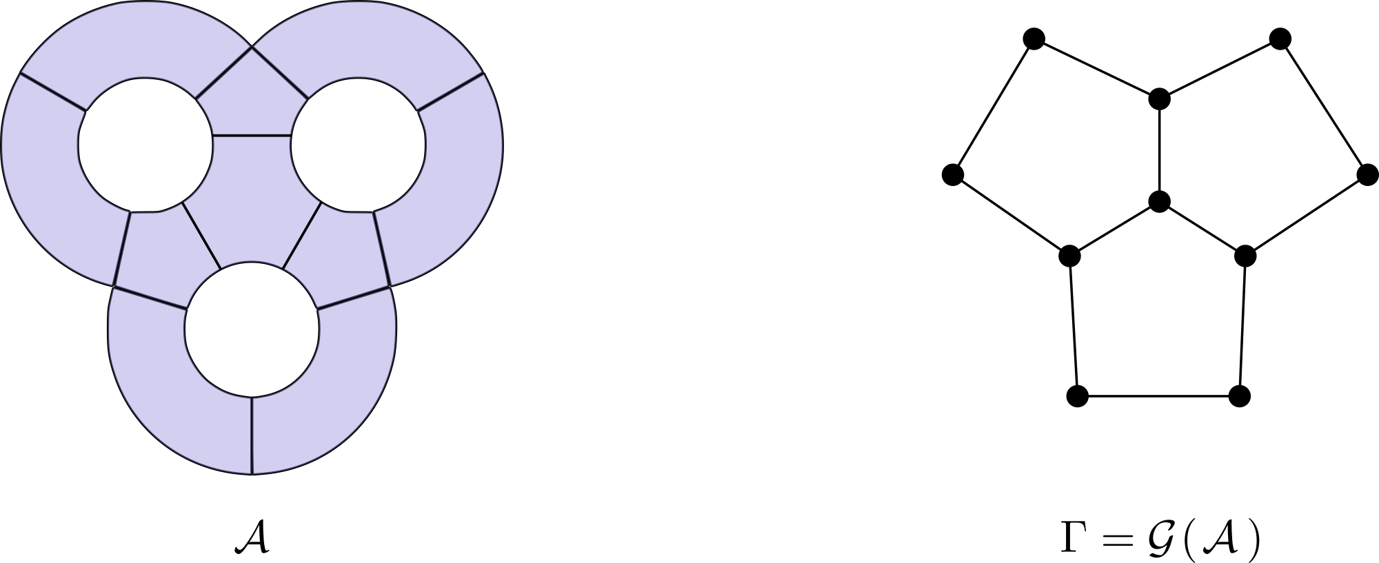
This multipartite entanglement problem can be expressed in the language of graph theory, where each subsystem is represented by a vertex and the connection between two subsystems is represented by an edge (figure 43). We focus on planar graphs. If $n_{h}$ is the number of holes in the graph, then $n_{h}+1=f$ , where $f$ is the number of faces (connected components) in the complement of the graph. In the above particular example (figure 43) the number of holes $n_{h}=3$ . For planar graphs, this multipartite information measure is related to the graph polynomial ${\beta}_{\Gamma}(x)$ evaluated at $x=-1$ , i.e.,

\displaystyle I^{N}_{\mathcal{A}}

\displaystyle=

\displaystyle-\Omega{\beta}_{\Gamma}(-1).

Using the graph polynomial, one can describe the vanishing of multipartite information measure $I^{N}_{\mathcal{A}}$ by showing that ${\beta}_{\Gamma}(-1)=0$ .

We summarize the results for various types of CSS (collection of subsystems) and their corresponding graphs in figure 44. We know that ${\beta}_{\Gamma}(-1)$ and the corresponding multipartite information measure are both non-zero for cycle graphs with at least $3$ vertices. This is robust against certain deformations like adding self-loops and nearest neighbor handle additions (rightmost figures in figure 44). On the other hand, this is zero (leftmost figures in figure 44) of path graph, a union of disjoint connected graphs, extra appendage, and short circuit.
Apart from applications to topological entanglement entropy, our graph-theoretic formalism has potential applications in machine learning [42, 55] and artificial intelligence [13, 15], both of which are data-driven methods with the potential to solve many complex problems by pattern recognition. Storing data and their interconnections are often represented in terms of a graph. Storing data in subgraphs can help drastically simplify the problem [20]. We hope to use the graph simplification procedure (obtained via graph coloring and the colored $\beta$ polynomial) to use in this context.

5.4. Emergence of Euler characteristic

Recall the total island count polynomial for an embedded graph $(\Gamma,\sigma)$ on $n$ vertices is given by

(5.4)

\beta_{\Gamma}(x)=\sum_{i=1}^{n}\Big(\sum_{\Gamma^{\prime}\in\mathscr{F}_{i}(\Gamma)}f_{\sigma}(\Gamma^{\prime})\Big)x^{i-1}=f_{\sigma}(\Gamma)x^{n-1}+\sum_{i=1}^{n-1}\Big(\sum_{\Gamma^{\prime}\in\mathscr{F}_{i}(\Gamma)}f_{\sigma}(\Gamma^{\prime})\Big)x^{i-1}.

This can be rewritten, recursively using (5.4), as

$\displaystyle\beta_{\Gamma}(x)$	$\displaystyle=$	$\displaystyle f_{\sigma}(\Gamma)x^{n-1}+\sum_{\Gamma^{\prime}\in\mathscr{F}_{n-1}(\Gamma)}f_{\sigma}(\Gamma^{\prime})x^{i-1}+\sum_{i=1}^{n-2}\Big(\sum_{\Gamma^{\prime}\in\mathscr{F}_{i}(\Gamma)}f_{\sigma}(\Gamma^{\prime})\Big)x^{i-1}$
	$\displaystyle=$	$\displaystyle f_{\sigma}(\Gamma)x^{n-1}+\sum_{\Gamma^{\prime}\in\mathscr{F}_{n-1}(\Gamma)}\Big(\beta_{\Gamma^{\prime}}(x)-\sum_{j=1}^{n-2}\Big(\sum_{\Gamma^{\prime\prime}\in\mathscr{F}_{j}(\Gamma^{\prime})}f_{\sigma}(\Gamma^{\prime\prime})\Big)x^{j-1}\Big)+\sum_{i=1}^{n-2}\Big(\sum_{\Gamma^{\prime}\in\mathscr{F}_{i}(\Gamma)}f_{\sigma}(\Gamma^{\prime})\Big)x^{i-1}$
	$\displaystyle=$	$\displaystyle f_{\sigma}(\Gamma)x^{n-1}+\sum_{\Gamma^{\prime}\in\mathscr{F}_{n-1}(\Gamma)}\beta_{\Gamma^{\prime}}(x)-\sum_{j=1}^{n-2}\Big(\sum_{\Gamma^{\prime}\in\mathscr{F}_{i}(\Gamma)}(n-j+1)f_{\sigma}(\Gamma^{\prime})\Big)x^{i-1}$

where the factor of $(n-j-1)$ appears because a subgraph $\Gamma^{\prime\prime}$ on $j$ vertices lies inside $n-j$ subgraphs with $n-1$ vertices. Iterating this we obtain

(5.5)

\beta_{\Gamma}(x)=f_{\sigma}(\Gamma)x^{n-1}+\sum_{\Gamma^{\prime}\in\mathscr{F}_{n-1}(\Gamma)}\beta_{\Gamma^{\prime}}(x)-\sum_{\Gamma^{\prime}\in\mathscr{F}_{n-2}(\Gamma)}\beta_{\Gamma^{\prime}}(x)+\cdots+(-1)^{n-2}\sum_{\Gamma^{\prime}\in\mathscr{F}_{1}(\Gamma)}\beta_{\Gamma^{\prime}}(x).

In particular, putting $x=-1$ , we conclude that the total island count for $\Gamma$ is, up to an additive factor of $\pm f_{\sigma}(\Gamma)$ , the alternating sum of the total island counts of its subgraphs.
For a planar graph $\Gamma$ , we may remove self-loops and similar adjacencies in order to compute $\beta_{\Gamma}(-1)$ .

Planar graphs have total island count zero if one of the following holds:
(a) it is disconnected (2.3)
(b) has at least three vertices and a pendant vertex (2.6)
(c) is a wedge sum of graphs (4.4)
(d) has a clean short circuit (Proposition 4.19).
We assume that $\Gamma$ is connected and does not satisfy (a)-(d). Let $v,e$ and $f$ denote the number of vertices, edges and faces of $\Gamma\hookrightarrow S^{2}$ respectively. The only contributions to $\beta_{\Gamma}(-1)$ come from
(i) $(-1)^{n}v$ , the last term in the right hand side (RHS) of (5.5)
(ii) $(-1)^{n-1}f$ , the first term in the RHS of (5.5)
(iii) $(-1)^{n-1}e$ , the second last term in the RHS of (5.5)
(iv) $\beta_{\Gamma^{\prime}}(-1)$ for subgraphs $\Gamma^{\prime}$ not satisfying (a)-(d).
The contributions from (iv) include signed counts of $k$ -cycles in $\Gamma$ . The contribution from (i) through (iii) is

(-1)^{n}(v-e-f)=(-1)^{n}(v-e+f)-(-1)^{n}2f=(-1)^{n}(\chi-2f),

where $\chi=2$ is the Euler characteristic of $S^{2}$ . In particular, if $c_{k}$ denotes the number of $k$ -cycles, then

(5.6)	$\displaystyle(-1)^{n}\beta_{\Gamma}(-1)$	$\displaystyle=$	$\displaystyle\chi-2f+\sum_{j=3}^{n-1}\sum_{\Gamma^{\prime}\in\mathscr{F}_{j}}(-1)^{j-1}\beta_{\Gamma^{\prime}}(-1)$
		$\displaystyle=$	$\displaystyle\chi-2f+\beta_{C_{3}}(-1)c_{3}+\sum_{j=4}^{n-1}\sum_{\Gamma^{\prime}\in\mathscr{F}_{j}}(-1)^{j-1}\beta_{\Gamma^{\prime}}(-1).$
		$\displaystyle=$	$\displaystyle\chi-2f+2c_{3}-((-2)c_{4}+2c_{K_{4}})+\sum_{j=5}^{n-1}\sum_{\Gamma^{\prime}\in\mathscr{F}_{j}}(-1)^{j-1}\beta_{\Gamma^{\prime}}(-1)$

where $c_{K_{4}}$ is the number of $K_{4}$ ’s in $\Gamma$ and $\beta_{K_{4}}(-1)=2$ . One can expand this further with a lot of care. For instance, the only graphs on $5$ vertices not satisfying (a)-(d) are of three types as depicted in figure 46. Thus, the contribution from $\mathscr{F}_{5}(\Gamma)$ would be counting induced subgraphs in $\Gamma$ of one of the types shown in figure 46 with weights $2,-2,-2$ and $-2$ respectively.

Figure 46. Graphs on

5

vertices with non-zero

\beta(-1)

For a general embedded graph $(\Gamma,\sigma)$ , $\sigma(\Gamma)$ need not give a triangulation of the surface. If we assume that $\Gamma$ has enough edges embedded appropriately such that each component of $\Sigma-\sigma(\Gamma)$ is a disk, then $f_{\sigma}(\Gamma)$ is the number of faces $f$ . If all self-loops in $\Gamma$ are homologically trivial and all similar adjacencies (of the same edge) are homotopic (to the corresponding edge), then (5.6) holds. A way to interpret (5.6) is the following rewriting of it.

(5.7)

(-1)^{n}\beta_{\Gamma}(-1)+\sum_{j=3}^{n-1}\sum_{\Gamma^{\prime}\in\mathscr{F}_{j}(\Gamma)}(-1)^{j}\beta_{\Gamma^{\prime}}(-1)=\chi-2f.

From a computational perspective (and certainly from a topological entanglement entropy point of view), we can recover $\chi-2f$ as the alternating sum of total island counts associated to all subgraphs of $\Gamma$ on at least $3$ vertices. In physics parlance, $\chi-2f$ is an emergent feature arising from computing topological entanglement entropy.

Appendix A Proof of Theorem 2.13

Definition A.1.

Let $A\subseteq[n]=\{1,2,\dots,n\}$ . Let us call a subset $B\subseteq A$ an island of $A$ on the line if there exist integers $i$ and $j$ such that $B=\{i,i+1,\dots,j\}$ and $i-1,j+1\notin A$ . Let $\mathcal{I}(A)$ denote the set of all islands of $A$ on the line and define $\mathcal{B}^{n}_{m}:=\sum_{|A|=m}|\mathcal{I}(A)|$ .

Definition A.2.

Let $A\subseteq[n]=\{1,2,\dots,n\}$ . Let us call a subset $B\subseteq A$ an island of $A$ on the circle if there exist integers $i$ and $j$ such that $B=\{i,i+1,\dots,j\}$ and $i-1,j+1\notin A$ . Here the addition is carried out mod $n$ . Let $\mathcal{J}(A)$ denote the set of all islands of $A$ on the circle and define $\mathcal{D}^{n}_{m}=\sum_{|A|=m}|\mathcal{J}(A)|$ .

Note that $\mathcal{D}^{n}_{m}=\mathcal{D}_{m}(C_{n})$ . We need some preliminary observations.

Lemma A.3.

The numbers $\mathcal{B}_{m}^{n}$ satisfy the following recurrence relation

(A.1)

\mathcal{B}_{m}^{n}=\mathcal{B}_{m}^{n-1}+\left(\mathcal{B}_{m-1}^{n-2}+{n-2\choose m-1}\right)+\dots+\left(\mathcal{B}^{n-m}_{1}+{n-m\choose 1}\right)+1.

Proof.

Let us consider a set $A\subset[n]$ of $m$ elements. Let $I$ be the island in $A$ containing $n$ . Then $|I|=r$ for some $0\leq r\leq m$ and the $r=0$ case takes into account that there may be no such island $I$ in $A$ .
We now count $\mathcal{B}^{n}_{m}$ in terms of $r$ . If we set $r=0$ , then $I=\varnothing$ and $A\subseteq[n-1]$ . This means that sum of all possible islands of all the $A$ ’s satisfying this case will be $\mathcal{B}^{n-1}_{m}$ . If we put $r=1$ , then the only possibility is $I=\{n\}$ . Therefore, it follows that $n\in A$ and $n-1\notin A$ , whence $A\setminus\{n\}\subseteq[n-2]$ (refer to the figure below)

As the total number of possible $A$ ’s is ${n-2\choose m-1}$ , the contribution of this case is given by

	$\displaystyle\sum_{\|A\|=m,n\in A,n-1\notin A}\|\mathcal{I}(A)\|$	$\displaystyle=\sum_{\|A\|=m,n\in A,n-1\notin A}(\|\mathcal{I}(A\setminus\{n\})\|+1)$
		$\displaystyle=\sum_{\|A\|=m,n\in A,n-1\notin A}\|\mathcal{I}(A\setminus\{n\})\|+{n-2\choose m-1}$
		$\displaystyle=\sum_{B\subseteq[n-2],\|B\|=m-1}\|\mathcal{I}(B)\|+{n-2\choose m-1}$
		$\displaystyle=\mathcal{B}_{m-1}^{n-2}+{n-2\choose m-1}.$

Let us now consider the general case, $|I|=r$ . In this case the only possibility is $I=\{n-r+1,n-r+2,\dots,n\}$ . It follows that $A\setminus I\subseteq[n-r-1]$ . As the total number of possible $A$ ’s is ${n-r-1\choose m-r}$ , the contribution of this case is given by

	$\displaystyle\sum_{\|A\|=m,I\subseteq A,n-r\notin A}\|\mathcal{I}(A)\|$	$\displaystyle=\sum_{\|A\|=m,I\subseteq A,n-r\notin A}(\|\mathcal{I}(A\setminus I)\|+1)$
		$\displaystyle=\sum_{\|A\|=m,I\subseteq A,n-r\notin A}\|\mathcal{I}(A\setminus I)\|+{n-r-1\choose m-r}$
		$\displaystyle=\sum_{B\subseteq[n-r-1],\|B\|=m-r}\|\mathcal{I}(B)\|+{n-r-1\choose m-r}$
		$\displaystyle=\mathcal{B}_{m-r}^{n-r-1}+{n-r-1\choose m-r}.$

Summing over all possible values of $r$ gives us the required result. ∎

A repeated use of Pascal’s triangle formula helps us simplify (A.1):

(A.2)

\mathcal{B}_{m}^{n}=\mathcal{B}_{m}^{n-1}+\mathcal{B}_{m-1}^{n-2}+\dots+\mathcal{B}_{1}^{n-m}+{n-1\choose m-1}.

Using (A.2), with $n$ replaced by $n-1$ , we obtain

\mathcal{B}^{n-2}_{m-1}+B^{n-3}_{m-2}+\dots+\mathcal{B}^{n-m}_{1}=\mathcal{B}^{n-1}_{m-1}-{n-2\choose m-2}.

Putting this in (A.2) and simplifying, we obtain

(A.3)

\mathcal{B}^{n}_{m}=\mathcal{B}^{n-1}_{m}+\mathcal{B}^{n-1}_{m-1}+{n-2\choose m-1}.

These $\mathcal{B}^{n}_{m}$ ’s obey a concrete formula, i.e.,

(A.4)

\mathcal{B}^{n}_{m}=(n-m+1){n-1\choose m-1}.

This follows from the fact that $\mathcal{B}^{n}_{m}$ and $(n-m+1){n-1\choose m-1}$ both satisfy the recurrence relation (A.3) and agree in the base case, i.e., $\mathcal{B}^{n}_{1}=(n-1+1).1=n$ .
We shall now give a recurrence relation for $\mathcal{D}^{n}_{m}$ in terms of $\mathcal{B}^{i}_{j}$ ’s.

Lemma A.4.

The numbers $\mathcal{D}^{n}_{m}$ satisfy the following recurrence relation:

(A.5)

\mathcal{D}^{n}_{m}=\mathcal{B}^{n}_{m}+m+\sum_{j=1}^{m-1}j\left(\mathcal{B}^{n-2-j}_{m-j}+{n-2-j\choose m-j}\right).

Proof.

Let us fix a set $A\subseteq[n]$ with $|A|=m$ . Let $I$ be the island in $A$ containing $n$ . The possibilities are $|I|=r$ for $0\leq r\leq m$ . First, let us consider the case $|I|=0$ . In this case, we have that $n\notin A$ . Therefore we are reduced to thinking of $A$ as a subset of the line with $n-2$ elements.

Hence, the total contribution of this case is $\mathcal{B}^{n-1}_{m}$ .
Let us now put $r=1$ . In this case the only possibility is $I=\{n\}$ and it must happen that $n\in A$ and $n-1,1\notin A$ . Hence $A\setminus\{n\}\subseteq[n-2]\setminus\{1\}$ (figure 49).

Note that the total number of possible $A$ ’s is ${n-3\choose m-1}$ . Therefore the contribution of this case is given by,

	$\displaystyle\sum_{\|A\|=m,n\in A,n-1,1\notin A}\|\mathcal{J}(A)\|$	$\displaystyle=\sum_{\|A\|=m,n\in A,n-1,1\notin A}(\|\mathcal{I}(A\setminus\{n\})\|+1)$
		$\displaystyle=\sum_{\|A\|=m,n\in A,n-1,1\notin A}\|\mathcal{I}(A\setminus\{n\})\|+{n-3\choose m-1}$
		$\displaystyle=\sum_{B\subseteq[n-2]\setminus\{1\},\|B\|=m-1}\|\mathcal{I}(B)\|+{n-3\choose m-1}$
		$\displaystyle=\mathcal{B}_{m-1}^{n-3}+{n-3\choose m-1}.$

Let us now consider the general case, $|I|=r$ . In this case there are $r$ many distinct possibilities of $I$ which are all symmetric, in the context of our counting problem. Without loss of generality, we can consider one of them and multiply its contribution by $r$ . So let us put $I=\{n-r+1,n-r+2,\dots,n\}$ . In particular, as $I\subseteq A$ is an island we must have $n-r,1\notin A$ . Hence $A\setminus I\subseteq[n-r-1]\setminus\{1\}$ . The total number of possible $A$ ’s is ${n-r-2\choose m-r}$ . Therefore, the contribution of such $A$ ’s is given by,

	$\displaystyle\sum_{\|A\|=m,I\subseteq A,n-r,1\notin A}\|\mathcal{J}(A)\|$	$\displaystyle=\sum_{\|A\|=m,I\subseteq A,n-r,1\notin A}(\|\mathcal{I}(A\setminus I)\|+1)$
		$\displaystyle=\sum_{\|A\|=m,I\subseteq A,n-r,1\notin A}\|\mathcal{I}(A\setminus I)\|+{n-r-2\choose m-r}$
		$\displaystyle=\sum_{B\subseteq[n-r-1]\setminus\{1\},\|B\|=m-r}\|\mathcal{I}(B)\|+{n-r-2\choose m-r}$
		$\displaystyle=\mathcal{B}_{m-r}^{n-r-2}+{n-r-2\choose m-r}.$

Therefore, the total contribution of this case is $r\Big(\mathcal{B}_{m-r}^{n-r-2}+{n-r-2\choose m-r}\Big)$ . Summing over $r$ gives us the required identity. ∎

Proof of Theorem 2.13.

Let us prove the second equality. Note that if

(A.6)

\sum_{j=0}^{m-1}(-1)^{j}\penalty\ (m-j){N\choose m-j}=N{N-2\choose m-1}

holds for $N$ and $m<N-1$ , then consider the sum (and its simplification)

$\displaystyle\sum_{j=0}^{m}(-1)^{j}\penalty\ (m+1-j){N\choose m+1-j}$	$\displaystyle=$	$\displaystyle(m+1){N\choose m+1}-\bigg(\sum_{j=0}^{m-1}(-1)^{j}\penalty\ (m-j){N\choose m-j}\bigg)$
	$\displaystyle=$	$\displaystyle(m+1){N\choose m+1}-N{N-2\choose m-1}$
	$\displaystyle=$	$\displaystyle N{N-2\choose m}.$

As (A.6) holds for $m=1$ and any $N$ , it holds for all $m$ and $N$ such that $1\leq m<N$ .
Instead of proving the first equality, we will show that $\mathcal{D}_{m}(C_{N})=N{N-2\choose m-1}$ . By rearranging the terms of right hand side of (A.5), we can see that,

	$\displaystyle\mathcal{D}^{n}_{m}=$	$\displaystyle\mathcal{B}^{n-1}_{m}+\Big[{n-3\choose m-1}+{n-4\choose m-2}+\dots+1\Big]$
		$\displaystyle+\Big[\mathcal{B}^{n-3}_{m-1}+\big(\mathcal{B}^{n-4}_{m-2}+{n-4\choose m-2}\big)+\dots+\big(\mathcal{B}^{n-m-1}_{1}+{n-m-1\choose 1}\big)+1\Big]$
		$\displaystyle+\Big[\mathcal{B}^{n-4}_{m-2}+\big(\mathcal{B}^{n-5}_{m-3}+{n-5\choose m-3}\big)+\dots+\big(\mathcal{B}^{n-m-1}_{1}+{n-m-1\choose 1}\big)+1\Big]+\cdots$
		$\displaystyle+\Big[\mathcal{B}^{n-m-2}_{2}+\big(\mathcal{B}^{n-m-1}_{1}+{n-m-1\choose 1}\big)+1\Big]+[\mathcal{B}^{n-m-1}_{1}+1].$

By repeatedly using (A.1) we obtain that

	$\displaystyle\mathcal{D}^{n}_{m}$	$\displaystyle=\mathcal{B}^{n-1}_{m}+{}^{n-2\choose m-1}+\mathcal{B}^{n-2}_{m-1}+\mathcal{B}^{n-3}_{m-2}+\dots+\mathcal{B}^{n-m-1}_{2}+\mathcal{B}^{n-m}_{1}$
		$\displaystyle=\left[\mathcal{B}^{n-1}_{m}+\mathcal{B}^{n-2}_{m-1}+\dots+\mathcal{B}^{n-m}_{1}+{n-1\choose m-1}\right]+{n-2\choose m-1}-{n-1\choose m-1}$
		$\displaystyle=\mathcal{B}^{n}_{m}-{n-2\choose m-2}.$

Finally, using (A.4), we may simplify the above formula to get our desired formula. ∎

References

[1] J. A. Barnes and F. Harary, Graph theory in network analysis, Social networks, 5 (1983), pp. 235–244.
[2] F. Battiston, E. Amico, A. Barrat, G. Bianconi, G. F. de Arruda, I. Franceschiello, B. Iacopini, S. Kéfi, V. Latora, Y. Moreno, Y. M. Murray, T. P. Peixoto, V. F., and G. Petri, The physics of higher-order interactions in complex systems, Nature Physics, 17 (2021), pp. 1093–1098.
[3] B. C. Bernhardt, L. Bonilha, and D. W. Gross, Network analysis for a network disorder: the emerging role of graph theory in the study of epilepsy, Epilepsy & Behavior, 50 (2015), pp. 162–170.
[4] S. M. Bhattacharjee, M. Mj, and A. Bandyopadhyay, Topology and Condensed Matter Physics, vol. 19, Springer, 2017.
[5] N. Biggs, N. L. Biggs, and B. Norman, Algebraic graph theory, no. 67, Cambridge university press, 1993.
[6] B. Bollobás, Modern graph theory, vol. 184 of Graduate Texts in Mathematics, Springer-Verlag, New York, 1998.
[7] S.-C. Chang and R. Shrock, Weighted graph colorings, J. Stat. Phys., 138 (2010), pp. 496–542.
[8] N. Deo, Graph theory with applications to engineering and computer science, Courier Dover Publications, 2017.
[9] S. Derrible and C. Kennedy, Network analysis of world subway systems using updated graph theory, Transportation Research Record, 2112 (2009), pp. 17–25.
[10] E. Fonda, K. R. Sreenivasan, and D. P. Lathrop, Reconnection scaling in quantum fluids, PNAS, 116 (2019), pp. 1924–1928.
[11] C. Fortuin and P. Kasteleyn, On the random-cluster model: I. introduction and relation to other models, Physica, 57 (1972), pp. 536–564.
[12] C. Godsil and G. F. Royle, Algebraic graph theory, vol. 207, Springer Science & Business Media, 2001.
[13] A. Ibeas and M. de la Sen, Artificial intelligence and graph theory tools for describing switched linear control systems, Applied Artificial Intelligence, 20 (2006), pp. 703–741.
[14] Y. Ihara, On discrete subgroups of the two by two projective linear group over p-adic fields, Journal of the Mathematical Society of Japan, 18 (1966), pp. 219–235.
[15] G. N. Kannaiyan, B. Pappula, and R. Veerubommu, A review on graph theory in network and artificial intelligence, in Journal of Physics: Conference Series, vol. 1831, IOP Publishing, 2021, p. 012002.
[16] P. Kapitza, Dynamic stability of a pendulum when its point of suspension vibrates, Soviet Phys. JETP, 21 (1951), pp. 588–597.
[17] M. Kardar, Statistial Physics of Fields, Cambridge University Press, 2012.
[18] A. Kitaev, Fault-tolerant quantum computation by anyons, Annals of Physics, 303 (2003), pp. 2–30.
[19] A. Kitaev and J. Preskill, Topological entanglement entropy, Phys. Rev. Lett., 96 (2006), p. 110404.
[20] E. Ko, M. Kang, H. J. Chang, and D. Kim, Graph-theory based simplification techniques for efficient biological network analysis, in 2017 IEEE Third International Conference on Big Data Computing Service and Applications (BigDataService), IEEE, 2017, pp. 277–280.
[21] S. Lal, On transport in quantum hall systems with constrictions, Europhys. Lett., 80 (2007), p. 17003.
[22] , Transport through constricted quantum hall edge systems: Beyond the quantum point contact, Phys. Rev. B, 77 (2008), p. 035331.
[23] M. Levin and X.-G. Wen, Detecting topological order in a ground state wave function, Phys. Rev. Lett., 96 (2006), p. 110405.
[24] I. Lifshitz, Anomalies of electron characteristics of a metal in the high pressure region, Sov. Phys. JETP, 11 (1960), pp. 1130–1135.
[25] A. Majeed and I. Rauf, Graph theory: A comprehensive survey about graph theory applications in computer science and social networks, Inventions, 5 (2020), p. 10.
[26] A. Mukherjee and S. Lal, Scaling theory for mott-hubbard transitions-i: T=0 phase diagram of the $1/2$ -filled hubbard model, New J. Phys., 22 (2020), p. 063007.
[27] , Scaling theory for mott-hubbard transitions-ii: Quantum criticality of the doped mott insulator, New J. Phys., 22 (2020), p. 063008.
[28] , Unitary renormalisation group for correlated electrons-i: a tensor network approach, Nucl. Phys. B, 960 (2020), p. 115170.
[29] , Unitary renormalisation group for correlated electrons-ii: insights on fermionic criticality, Nucl. Phys. B, 960 (2020), p. 115163.
[30] , Superconductivity from repulsion in the doped 2d electronic hubbard model: an entanglement perspective, arXiv preprint arXiv:2003.06118, accepted for publication in J. Phys. Cond. Mat., (2022).
[31] A. Mukherjee, A. Mukherjee, N. S. Vidhyadhiraja, A. Taraphder, and S. Lal, Unveiling the kondo cloud: Unitary renormalization-group study of the kondo model, Phys. Rev. B, 105 (2022), p. 085119.
[32] A. Mukherjee, S. Patra, and S. Lal, Fermionic criticality is shaped by fermi surface topology: a case study of the tomonaga-luttinger liquid, Journal of High Energy Physics, 04 (2021), p. 148.
[33] S. Pal, A. Mukherjee, and S. Lal, Correlated spin liquids in the quantum kagome antiferromagnet at finite field: a renormalization group analysis, New Journal of Physics, 21 (2019), p. 023019.
[34] S. Patra, S. Basu, and S. Lal, Unveiling topological order through multipartite entanglement, arXiv, (2021).
[35] S. Patra and S. Lal, Origin of topological order in a cooper-pair insulator, Phys. Rev. B, 104 (2021), p. 144514.
[36] M. Peskin and D. Schroeder, An Introduction to Quantum Field Theory, Addison-Wesley, 1995.
[37] F. Pollmann, A. M. Turner, E. Berg, and M. Oshikawa, Entanglement spectrum of a topological phase in one dimension, Phys. Rev. B, 81 (2010), p. 064439.
[38] R. B. Potts, Some generalized order-disorder transformations, Mathematical Proceedings of the Cambridge Philosophical Society, 48 (1952), p. 106–109.
[39] J. G. Ratcliffe, S. Axler, and K. Ribet, Foundations of hyperbolic manifolds, vol. 149, Springer, 1994.
[40] F. Riaz and K. M. Ali, Applications of graph theory in computer science, in 2011 Third International Conference on Computational Intelligence, Communication Systems and Networks, IEEE, 2011, pp. 142–145.
[41] J. Scott, Social network analysis, Sociology, 22 (1988), pp. 109–127.
[42] G. Srinivasan, J. D. Hyman, D. A. Osthus, B. A. Moore, D. O’Malley, S. Karra, E. Rougier, A. A. Hagberg, A. Hunter, and H. S. Viswanathan, Quantifying topological uncertainty in fractured systems using graph theory and machine learning, Scientific reports, 8 (2018), pp. 1–11.
[43] J. D. Stasheff, Homotopy associativity of h-spaces. i, Transactions of the American Mathematical Society, 108 (1963), pp. 275–292.
[44] , Homotopy associativity of h-spaces. ii, Transactions of the American Mathematical Society, 108 (1963), pp. 293–312.
[45] S. H. Strogatz, Nonlinear dynamics and chaos: with applications to physics, biology, chemistry, and engineering, CRC press, 2018.
[46] P. M. Tam, M. Klaassen, and C. L. Kane, Topological multipartite entanglement in a fermi liquid, arXiv/2204.06559, (2022).
[47] W. T. Tutte, A contribution to the theory of chromatic polynomials, Canadian journal of mathematics, 6 (1954), pp. 80–91.
[48] W. T. Tutte, On dichromatic polynomials, Journal of Combinatorial Theory, Series A, 2 (1967), pp. 301–320.
[49] L. Van Hove, The occurrence of singularities in the elastic frequency distribution of a crystal, Phys. Rev., 89 (1953), pp. 1189–1193.
[50] G. Volovik, Quantum phase transitions from topology in momentum space, Springer Lecture Notes in Physics, 718 (2007), pp. 31–73.
[51] , Topological lifshitz transitions, Low Temperature Physics, 43 (2017), pp. 47–55.
[52] X.-G. Wen, Topological order: From long-range entangled quantum matter to a unified origin of light and electrons, ISRN Condensed Matter Physics, 2013 (2013), p. 198710.
[53] , Colloquium: Zoo of quantum-topological phases of matter, Reviews of Modern Physics, 89 (2017), p. 041004.
[54] , Choreographed entanglement dances: Topological states of quantum matter, Science, 363 (2019), p. eaal3099.
[55] W. Zhang, J. Chien, J. Yong, and R. Kuang, Network-based machine learning and graph theory algorithms for precision oncology, NPJ precision oncology, 1 (2017), pp. 1–15.

	$\displaystyle\sum_{\|A\|=m,n\in A,n-1\notin A}\|\mathcal{I}(A)\|$	$\displaystyle=\sum_{\|A\|=m,n\in A,n-1\notin A}(\|\mathcal{I}(A\setminus\{n\})\|+1)$
		$\displaystyle=\sum_{\|A\|=m,n\in A,n-1\notin A}\|\mathcal{I}(A\setminus\{n\})\|+{n-2\choose m-1}$
		$\displaystyle=\sum_{B\subseteq[n-2],\|B\|=m-1}\|\mathcal{I}(B)\|+{n-2\choose m-1}$
		$\displaystyle=\mathcal{B}_{m-1}^{n-2}+{n-2\choose m-1}.$

	$\displaystyle\sum_{\|A\|=m,I\subseteq A,n-r\notin A}\|\mathcal{I}(A)\|$	$\displaystyle=\sum_{\|A\|=m,I\subseteq A,n-r\notin A}(\|\mathcal{I}(A\setminus I)\|+1)$
		$\displaystyle=\sum_{\|A\|=m,I\subseteq A,n-r\notin A}\|\mathcal{I}(A\setminus I)\|+{n-r-1\choose m-r}$
		$\displaystyle=\sum_{B\subseteq[n-r-1],\|B\|=m-r}\|\mathcal{I}(B)\|+{n-r-1\choose m-r}$
		$\displaystyle=\mathcal{B}_{m-r}^{n-r-1}+{n-r-1\choose m-r}.$

	$\displaystyle\sum_{\|A\|=m,n\in A,n-1,1\notin A}\|\mathcal{J}(A)\|$	$\displaystyle=\sum_{\|A\|=m,n\in A,n-1,1\notin A}(\|\mathcal{I}(A\setminus\{n\})\|+1)$
		$\displaystyle=\sum_{\|A\|=m,n\in A,n-1,1\notin A}\|\mathcal{I}(A\setminus\{n\})\|+{n-3\choose m-1}$
		$\displaystyle=\sum_{B\subseteq[n-2]\setminus\{1\},\|B\|=m-1}\|\mathcal{I}(B)\|+{n-3\choose m-1}$
		$\displaystyle=\mathcal{B}_{m-1}^{n-3}+{n-3\choose m-1}.$

	$\displaystyle\sum_{\|A\|=m,I\subseteq A,n-r,1\notin A}\|\mathcal{J}(A)\|$	$\displaystyle=\sum_{\|A\|=m,I\subseteq A,n-r,1\notin A}(\|\mathcal{I}(A\setminus I)\|+1)$
		$\displaystyle=\sum_{\|A\|=m,I\subseteq A,n-r,1\notin A}\|\mathcal{I}(A\setminus I)\|+{n-r-2\choose m-r}$
		$\displaystyle=\sum_{B\subseteq[n-r-1]\setminus\{1\},\|B\|=m-r}\|\mathcal{I}(B)\|+{n-r-2\choose m-r}$
		$\displaystyle=\mathcal{B}_{m-r}^{n-r-2}+{n-r-2\choose m-r}.$